Topological origins of a bi-parameter periodicity hub for the Rössler attractor

Abstract

We explore the dynamical and topological characteristics of the Rössler system that lead to the existence of a periodicity hub and nested spiral in codimension-2 parameter space. We find that the hub shape is a consequence of conjugacy between the Rössler system and unimodal maps in the two-branch region of the parameter space. The nested spiral structure is a consequence of a topological feature of the Rössler system that has not been noted previously. We outline this mechanism and detail the spiral transition for the symbolic sequence of orbits up to period seven.

Recent work has focused attention on the appearance of nested spirals and so called “shrimp” within the codimension-2 parameter space of a number of dissipative systems. First noted by Bonatto and Gallas in 2008 Bonatto and Gallas (2008), these hubs have been the focus of number of investigations since Barrio et al. (2009); Gallas (2010); Ramírez-Ávila and a.C. Gallas (2010); Freire and Gallas (2010); Barrio et al. (2011); Shilnikov and Shilnikov (2011); Vitolo et al. (2011).

The occurrence of these hubs is easily seen in a mapping of the global Lyapunov exponents in codimension-2 parameter space (Figure 1). We focus on a hub found in the Rössler system. The hubs for this system have been studied for a number of different parameter values Barrio et al. (2009). We chose to work with the parameter space of the Rössler system where $b=0.2$ and $(a,c)$ vary. It can be shown that the shape of this hub is robust with a variation of $b$, drifting rightwards and slightly downwards in the $a,b$ parameter plane as $b$ increases from $0.2$ through $2.0$.

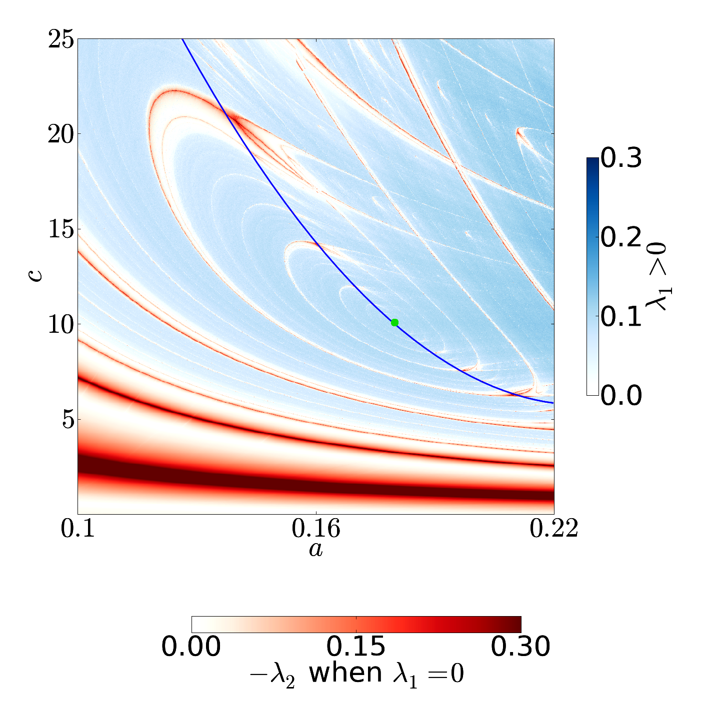
Figure 1: Lyapunov diagram for the Rössler system, close up of primary spiral hub. Green center dot (color online) indicates the center of the spiral hub. Dark blue line indicates a best-fit curve for the partition of the primary hub by the appearance of “shrimp”. Blue coloration reflects the intensity of the first Lyapunov exponent and corresponds to chaotic regions, red coloring reflects that of the negative of the second exponent when $\lambda_{1}=0$ and corresponds to stable regions. Lyapunov exponents were calculated on a 1000x1000 grid using the LESNLS software package Dieci et al. (2011).

The equations for the Rössler system Rössler (1976) are,

$$\dot{x}=-y-z,\ \ \dot{y}=x+ay,\ \ \dot{z}=b+z\left({x-c}\right)$$ (1)

While this system was first designed as a model for chaos, with no practical use in mind, numerous dynamical systems in fields such as chemistry, electronics, biology, and lasers have been found to exhibit behavior conjugate to that of the Rössler system Gilmore and Lefranc (2002).

In Figure 1, we draw an approximate best-fit curve linking the centers of so called “shrimp” structures along a line which corresponds to a transition from “spiral” (the return-map of the Rössler attractor has two branches) to “screw-like” structure in the Rössler attractor, which corresponds to the branched-manifold describing the Rössler attractor obtaining a third branch and the return-map appearing bimodal with two critical points. We call this line the Topological Transition Line and write this particular line as $TTL^{2}_{3}$ to indicate the transition from needing a branched-manifold with two branches to one with three branches as we move in parameter space from left to right Gilmore (1998). In agreement with previous estimates Barrio et al. (2011), we find the center of the primary spiral hub to be numerically located at approximately $(a,c)=(0.1798,10.3084)$ which corresponds to a homoclinic bifurcation point, the only such point along $TTL^{2}_{3}$ Bonatto and Gallas (2008).

We first wish to understand the smooth structure left of the $TTL^{2}_{3}$, and we do so by assuming topological conjugacy between the Rössler system and unimodal maps for judiciously selected slices of parameter space. That is, while the return map for the Rössler attractor appears conjugate with unimodal maps left of $TTL^{2}_{3}$, we seek a more specific conjugacy–that of the spectrum of stable periodic orbits. For this purpose, we will compare the Rössler system with the most widely studied unimodal map. The Logistic Map is described by the equation $L(x_{n},r)=x_{n+1}\equiv rx_{n}\left(1-x_{n}\right)$. A method of analytically detecting periodic windows in the general class of Logistic type maps was introduced by the seminal work of Metropolis et al. in 1973 Metropolis and Stein (1973), and rediscovered by Jensen and Myers in 1985 Jensen and Myers (1985); Eidson et al. (1986). In order to locate windows of stability, we can study the iterations of the critical point. Whenever one of these iterations of the critical point intersects the critical point, we are assured of the existence of a super-stable periodic orbit which corresponds to one of the windows of stability seen in the Logistic Map’s bifurcation diagram. These iterations of the critical point “scar” the bifurcation diagram as continuous “caustics” and stand out due to a higher concentration of “hits” around these points. A further advantage of the caustic method is that this method also describes the symbolic encoding of the super-stable orbits Metropolis and Stein (1973). Similar caustics are seen in bifurcation diagrams taken for the Rössler system, but not necessarily with the same patterns as in the Logistic Map.

The apparent conjugacy between the Rössler bifurcation diagram, and that of the Logistic Map, has not been commonly noted (see Letellier 1995 Letellier et al. (1995) for an exception). This is likely due to the fact that this similarity can only be found if one takes a slice through parameter space that is properly oriented with regards to periodicity conjugacy requirements between the maps. In order to judiciously select a slice in parameter space through which we can assume topological conjugacy with the spectrum of stable periodic orbits in unimodal dynamics, we note that the main conjugacy requirements of the Logistic Map will be

• Unimodal structure.

• An initial period-1 orbit that undergoes a period doubling cascade and then transitions to chaos upon reaching the Feigenbaum point.

• The attractor evolves until it makes contact with a fixed point.

The Rössler system matches these requirements in a specific region,

• Unimodal structure: due to the highly dissipative nature of the Rössler system, its return map has a unimodal nature in the regions left of $TTL^{2}_{3}$.

• The Rössler system undergoes an Andronov-Hopf Bifurcation, which leads to a period-1 limit cycle that undergoes a period-doubling cascade as we get closer to $TTL^{2}_{3}$ in parameter space.

• The Rössler system has a homoclinic bifurcation curve (a thin parabola shape), the tip of which lies on $TTL^{2}_{3}$ Bonatto and Gallas (2008). The attractor makes contact with its fixed point in the form of a homoclinic orbit at this point.

We treat the Rössler system as if it were fully topologically conjugate to the Logistic Map for any line in the parameter space which begins at the Andronov-Hopf Bifurcation and terminates at the homoclinic point on the $TTL^{2}_{3}$ where the Rössler attractor first makes contact with its central fixed point. This results in the shape of the hub left of $TTL^{2}_{3}$ tracing out the shape of the Andronov-Hopf bifurcation curve.

In Figure 2, we draw an example of two such slices of parameter space that will fulfill these conjugacy requirements, $L1$ and $L2$. We find that their bifurcation diagram is qualitatively similar to that of the Logistic map, and furthermore, we tested this assumption by numerically recreating the first seven caustics in these bifurcation diagrams. At least up to period seven and likely so for higher periods, the order of periodic orbits in the Rössler system as we move along these lines is conjugate with that of the Logistic Map.

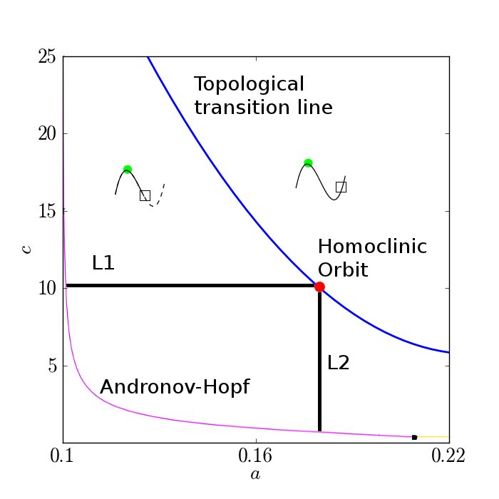
Figure 2: Parameter space diagram with Andronov-Hopf curve calculated using PyCONT/AUTO Clewley RH et al. (2007); Doedel and Oldeman (2009). Lines $L1$ and $L2$ originate from the period-1 limit cycle created after the Andronov-Hopf bifurcation of the Rössler attractor and terminate at a Homoclinic bifurcation point on the curve marking the topological transition from two to three branches in the branched manifold. The order of stable periodic orbits seen along these lines are conjugate to those seen in the Logistic map up to at least period seven and likely for much higher periods. We exclude the continuation of the homoclinic bifurcation curve into the three-branch region for simplicity.

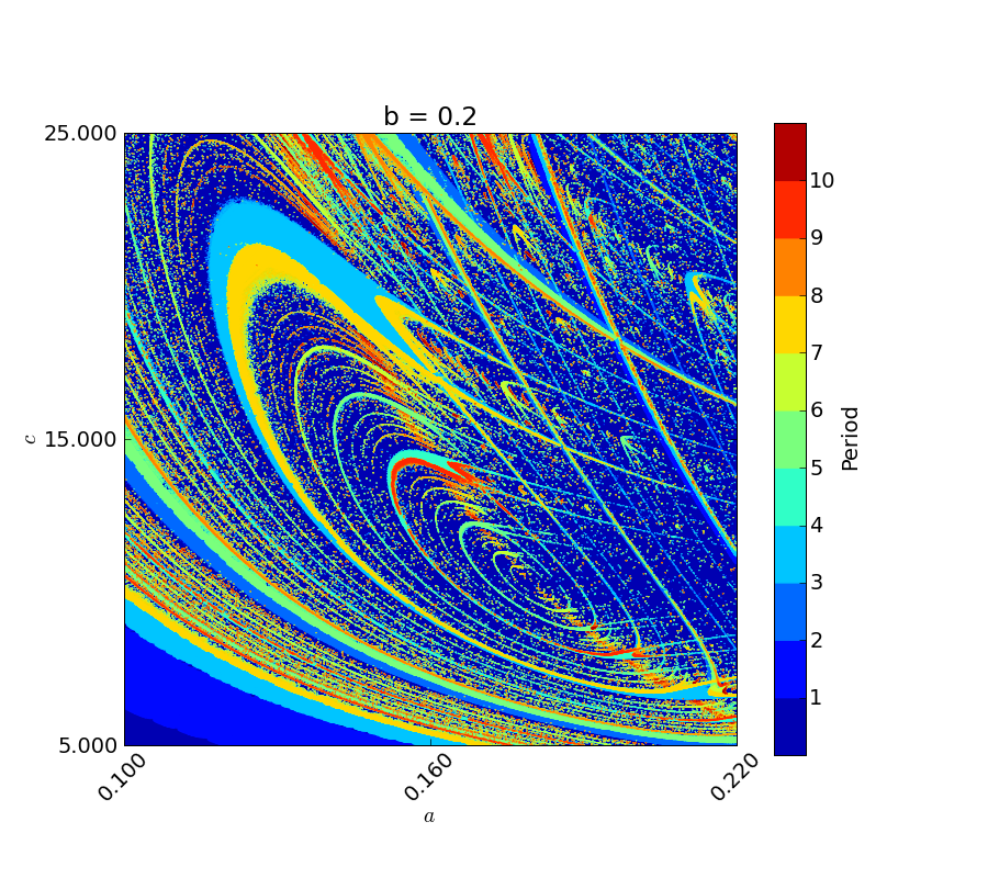
Figure 3: Periodicity calculations for the codimensional-2 parameter space of the Rössler attractor, for $b=0.2$, $a\in(0.1,0.22)$, $c\in(5.0,25.0)$. Darkest blue corresponds to divergent or chaotic behavior.

To further test these assumptions, we partitioned parameter space around the spiral hub into a 5000 by 5000 grid and applied a periodicity detection algorithm for each point. We color code the periods, up to period 11, producing an extensive periodicity graph in Figure 3 which shows that the periodicity is structured as predicted.

Finally, we can see that by continuity, this ordering of periods also determines the order of periods of the shrimp structures along the $TTL^{2}_{3}$. At the center of these shrimps, one finds a degenerate super-stable state which corresponds to the fact that at these points two intersecting parabola-shaped regions of super-stable periodicity contain both critical points simultaneously Gallas (1994). Careful consideration of the conditions at the intersection of the topological regions will help us understand why the shrimp line up along the transition curve. These stable regions represent iterations of at least one critical point of the return-map. The first two iterations of the critical point mark the borders of the range of possible iterations. As we pass through $TTL^{2}_{3}$ in phase space from left to right, the Rössler’s state-space return map grows a third branch. At $TTL^{2}_{3}$, the edge of the second branch is precisely the second critical point of the bimodal map in the branch-3 region.

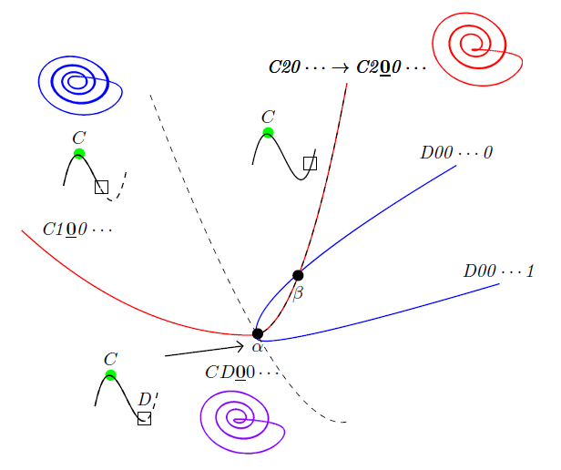
Figure 4: Anatomy of a generic “mutant shrimp” along the largest spiral. The symbolic string describing these orbits will be dominated by zeros. The center of the shrimp structure corresponds to a doubly-superstable orbit which includes both critical points. Each parabola corresponds to a variation of this orbit in which only one of the critical points is on the orbit. Due to the topological mechanism responsible for the periodicity transition, this shrimp has one tail which originates as a lower period and transitions to higher period before crossing $TTL^{2}_{3}$.

The shrimp along the $TTL^{2}_{3}$ and above the focal point behave as we would expect in the bimodal regime Gallas (1994). One of the “tails” of each of the shrimp points downward back towards the hub. This “tail” joins a shrimp below the focal point which has a different period. We call these “mutant shrimp” and have detected the periodicity transition to happen very close to $TTL^{2}_{3}$ (Figures 3 and 4).

Directly related to these structures is the question of the source of the nested periodicity spirals. These spirals are due to a previously unnoticed topological feature of the Rössler system.

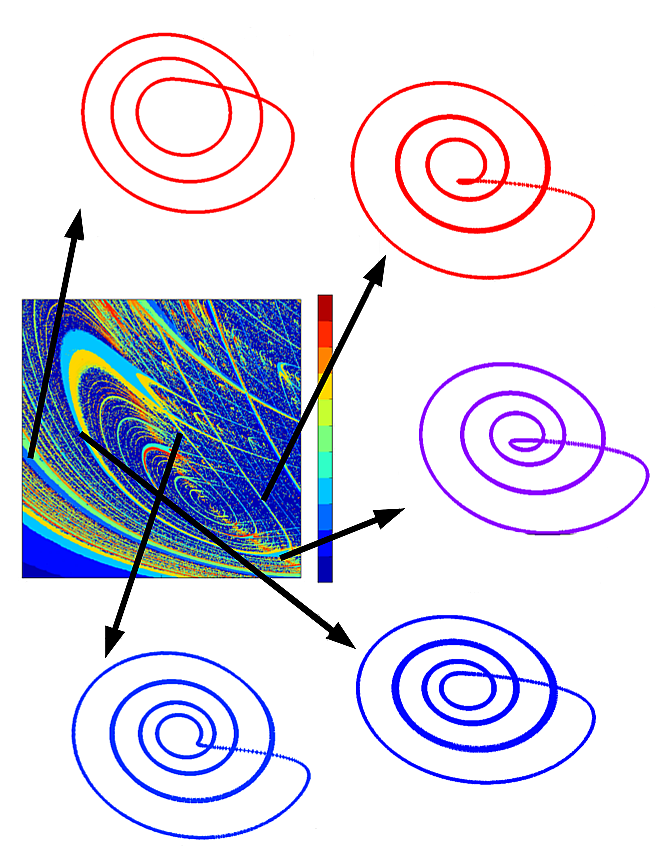
Figure 5: As we trace the periodicity spiral around in parameter space, clockwise from lower to higher period, the third branch of branched-manifold in state space is reinjected on the plane of the attractor at an angle that varies clockwise around the fixed-point, merging with the second branch as it crosses the $TTL^{2}_{3}$ from right to left.

The branched-manifold describing the Rössler system has been typically assumed to have a standard shape in which all branches are redeposited onto the main plane of the attractor at approximately the same position. We find that this is not the case for a small range of values in codimension-2 parameter space. In particular, as we move around one of the spiral features in the hub in parameter space, we find that in state space, the position at which the third branch is deposited on the main plane of the attractor rotates around the fixed point. Figure 5 shows this clearly for the spiral transition from period three to period four. As we follow a stable periodic orbit clockwise around the central spiral hub from lower periodicity to higher periodicity, the angle of deposit also rotates clockwise around the central dynamical fixed point in state space. Like a long chain being deposited in a circular way on a flat surface, the number of turns of the chain on the flat surface increases as we follow the periodicity regions as they spiral in towards the center of the spiral hub. As we cross $TTL^{2}_{3}$ following these spirals, the third branch “collapses” back onto the second branch, and the cycle starts over. This results in the transition between lower to higher period happening very rapidly near the shrimp along the bottom section of $TTL^{2}_{3}$ below the homoclinic point.

Following these spirals inwards, we find that the new points on an orbit are deposited on the inner-most region of the attractor, winding the attractor closer and closer to its fixed point until it makes full contact at the homoclinic bifurcation.

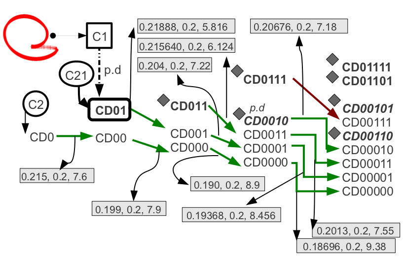
Figure 6: Symbol sequences in the nested spiral hub up to period seven. The orbits listed in each column are in the order that they appear in unimodal mappings Gilmore (1998). Green arrows indicate orderings which have been matched both by looking at the structure in state space, and by matching the symbol sequence of the corresponding transitions in parameter space. The transition $CD0111\rightarrow CD00111$ has only been confirmed by visually inspecting the attractor. Orbits in bold originate from isolated shrimp off of $TTL^{2}_{3}$ within the branch-3 side. The attached gray boxes indicate the approximate position of the corresponding mutant shrimp in parameter space.

Knowing this new mechanism, we can predict the symbolic sequence of orbits along a spiral. We must have that the critical point associated with the unimodal map on the branch-2 side of $TTL^{2}_{3}$, which we label $C$, is always part of the symbolic sequence along this spiral. This is due to the fact that the spiral region is continuous and crosses over the branch-2 side where the bimodal critical point, which we label $D$, is excluded. Thus both connected periods $p$ and $p+1$ will begin with symbol $C$. For example, we know that the period-four orbit $C100$ must transition into an orbit $C1X00$ after passing through the sequence $C200$ and returning to the $TTL^{2}_{3}$ since the third branch lays the new point on the orbit, where $X$ is either $0$ or $1$. Since we know that the new branch is deposited on the inner region of the main plane of the attractor, this new symbol will be a $0$, and so we have the transition from $C100\rightarrow C200\rightarrow C1000$. We have traced the trains for a number of orbits (Figure 6) which follow this general algorithm, though we note that higher periods will have a more complicated algorithm. We also find that the orbit $CD0$ is connected with an orbit $C2$ inside the branch-3 region, and $CD01$ has been found to be connected to an orbit $C21$ also from this region. Finally, we note that $CD01$ is the period-double of the orbit $C1$ which itself is connected to a period-one orbit in the branch-3 region which transitions to the orbit $C1$ by the same mechanism outlined in this report. The shape of this period-1 orbit is outlined in the upper left of Figure 6 as it nears transition.

Orbits that can not originate within a spiral, because the would-be preceding orbit does not exist, instead originate from one of the isolated shrimp in the branch-3 side of parameter space, though they themselves are then the beginning point of a new spiral, resulting in a nested set of spirals.

References

- Bonatto and Gallas (2008) C. Bonatto and J. Gallas, Physical Review Letters 101, 2 (2008), ISSN 0031-9007,
- Barrio et al. (2009) R. Barrio, F. Blesa, and S. Serrano, Physica D: Nonlinear Phenomena 238, 1087 (2009), ISSN 01672789,
- Gallas (2010) J. Gallas, International Journal of Bifurcation and Chaos 20, 197 (2010), ISSN 0218-1274,
- Ramírez-Ávila and a.C. Gallas (2010) G. M. Ramírez-Ávila and J. a.C. Gallas, Physics Letters A 375, 143 (2010), ISSN 03759601,
- Freire and Gallas (2010) J. Freire and J. Gallas, Physical Review E 82, 3 (2010), ISSN 1539-3755,
- Barrio et al. (2011) R. Barrio, F. Blesa, S. Serrano, and A. Shilnikov, Physical Review E (2011),
- Shilnikov and Shilnikov (2011) A. Shilnikov and L. Shilnikov, J. Bifurcations and Chaos pp. 1–19 (2011),
- Vitolo et al. (2011) R. Vitolo, P. Glendinning, and J. Gallas, Physical Review E 84, 1 (2011), ISSN 1539-3755,
- Dieci et al. (2011) L. Dieci, M. S. Jolly, and E. S. Van Vleck, Journal of Computational and Nonlinear Dynamics 6, 011003 (2011), ISSN 15551423,
- Rössler (1976) O. Rössler, Physics Letters A 57, 397 (1976), ISSN 03759601,
- Gilmore and Lefranc (2002) R. Gilmore and M. Lefranc, The Topology of Chaos: Alice in Stretch and Squeezeland (John Wiley & Sons, Limited, 2002), ISBN 9783527410675,
- Gilmore (1998) R. Gilmore, Reviews of Modern Physics 70, 1455 (1998),
- Metropolis and Stein (1973) N. Metropolis and M. Stein, Journal of Combinatorial Theory, 15, 25 (1973), ISSN 00973165,
- Jensen and Myers (1985) R. Jensen and C. Myers, Physical Review A 32, 1222 (1985),
- Eidson et al. (1986) J. Eidson, S. Flynn, C. Holm, D. Weeks, and R. Fox, Physical Review A 33, 2809 (1986),
- Letellier et al. (1995) C. Letellier, P. Dutertre, and B. Maheu, Chaos (Woodbury, N.Y.) 5, 271 (1995), ISSN 1089-7682,
- Clewley RH et al. (2007) Clewley RH, Sherwood WE, LaMar MD, and Guckenheimer JM, PyDSTool, a software environment for dynamical systems modeling (2007),
- Doedel and Oldeman (2009) E. J. Doedel and B. E. Oldeman (2009),
- Gallas (1994) J. Gallas, Physica A: Statistical Mechanics and its Applications 202, 196 (1994)