Pion production in nucleon-nucleon collisions in chiral effective field theory: next-to-next-to-leading order contributions

Abstract

A complete calculation of the pion-nucleon loops that contribute to the transition operator for $NN\to NN\pi$ up-to-and-including next-to-next-to-leading order (N²LO) in chiral effective field theory near threshold is presented. The evaluation is based on the so-called momentum counting scheme, which takes into account the relatively large momentum of the initial nucleons inherent in pion-production reactions. We show that the significant cancellations between the loops found at next-to-leading order (NLO) in the earlier studies are also operative at N²LO. In particular, the $1/m_{N}$ corrections (with $m_{N}$ being the nucleon mass) to loop diagrams cancel at N²LO, as do the contributions of the pion loops involving the low-energy constants $c_{i}$, $i=1\ldots 4$. In contrast to the NLO calculation however, the cancellation of loops at N²LO is incomplete, yielding a non-vanishing contribution to the transition amplitude. Together with the one-pion exchange tree-level operators, the loop contributions provide the long-range part of the production operator. Finally, we discuss the phenomenological implications of these findings. In particular, we find that the amplitudes generated by the N²LO pion loops yield contributions comparable in size with the most important phenomenological heavy-meson exchange amplitudes.

I Introduction

The reaction $NN\to NN\pi$ has been extensively studied both theoretically and experimentally over the past decades. However, the near-threshold regime is still not yet fully understood. After the first high-quality data for $pp\to pp\pi^{0}$ IUCF1 became available (further experimental data can be found in, e.g., the review article hanhart04 , with the latest measurements in Refs. ANKEpi0 ; ANKEpi- ), it quickly became clear that the original models failed to reproduce the new data. For example, the model of Ref. koltunundreitan fell short by a factor of two for the reaction $pp\to d\pi^{+}$ and by an order of magnitude for $pp\to pp\pi^{0}$. Various attempts were made to identify the phenomenological mechanisms responsible for this discrepancy.

The first theoretical paper to explain quantitatively the cross section $pp\to pp\pi^{0}$ was Ref. Lee . The new contribution in Lee originated from the short ranged, irreducible currents constructed directly from the nucleon-nucleon potential. A phenomenological interpretation of this mechanism was provided in Ref. HGM , where the exchange of heavy mesons (mostly $\sigma$ and $\omega$) followed by a pion emission via a nucleon-antinucleon pair (the so-called z-mechanism) was calculated. The mechanism was also shown to provide the missing strength for $pp\to d\pi^{+}$ in Refs. Hpipl ; jounicomment . An alternative mechanism is based on the pion-nucleon rescattering diagram where the off-shell pion-nucleon amplitude plays a crucial role. It is well-known that the isoscalar pion nucleon scattering length is very small — see Refs. ourpid for its most recent determination — as a result of a cancellation of individually sizable terms which have different energy dependences. It therefore appeared natural that in the off-shell kinematics relevant for the pion production reaction the amplitudes are significantly enhanced. This mechanism was also shown to be capable of describing the experimental data in both $pp\to pp\pi^{0}$ eulogio ; unsers as well as $pp\to d\pi^{+}$ unserd reactions. At this point there was no way to decide which of the mechanisms described captures the correct physics.

Since pion interactions are largely controlled by the chiral symmetry of the strong interaction, one might naturally expect that chiral perturbation theory (ChPT) provides the proper tool to resolve the above mentioned discrepancy. However, the use of the standard ChPT power counting, which is based on the assumption that all relevant momenta are effectively of the order of the pion mass, was not very successful. The first calculations in this framework were done at tree level up to N²LO for both $pp\to pp\pi^{0}$ cohen ; park ; sato as well as for $pp\to d\pi^{+}$ rocha ; unserd . These studies revealed, in particular, that the discrepancy between theory and experiment increases for the neutral channel due to a destructive interference of the direct pion production and the isoscalar rescattering contributions at NLO in standard counting. In addition, some loop contributions at N²LO were found in Refs. DKMS ; Ando to be larger than the NLO contribution, revealing a problem regarding the convergence of the standard ChPT power counting.

It was soon realized that the large initial nucleon momentum at threshold $p$, $p=|\vec{p}\,|=\sqrt{m_{N}m_{\pi}}$, which is significantly larger than the pion mass $m_{\pi}$, requires the modification of the standard power counting. The corresponding expansion parameter in the new scheme is

$$\chi=p/\Lambda_{\chi}\simeq\ 0.4,$$ (1)

with $\Lambda_{\chi}$ being the chiral symmetry breaking scale of the order of 1 GeV. Here and in what follows, this power counting will be referred to as the momentum counting scheme (MCS). This modification was proposed in Refs. cohen ; rocha while the proper way to treat this scale was first presented in Ref. ch3body and implemented in Ref. HanKai , see Ref. hanhart04 for a review article. The MCS expansion is performed with two distinct parameters, namely the initial nucleon momentum $p$ and the pion mass $m_{\pi}$, where $m_{\pi}/p\sim p/\Lambda_{\chi}$. The pion loop diagrams start to contribute at a given order in the expansion parameter, which can be identified based on the power counting, and, unlike the standard ChPT power counting, continue to contribute at all higher MCS orders.

Due to the fact that the Delta-nucleon ($\Delta$-N) mass splitting is numerically of the order of $p$, the Delta-isobar should be explicitly included as a dynamical degree of freedom cohen . This general argument was confirmed numerically in phenomenological calculations jouni ; ourdelta ; ourpols , see also Refs. cohen ; rocha ; HanKai ; NNpiMenu where the effect of the $\Delta$ in $NN\to NN\pi$ was studied within chiral EFT. However, in this paper we focus on contributions from nucleons and pions only. The $\Delta$ degree of freedom will be included in a subsequent publication.

In the MCS, pion p-waves are given by tree level diagrams up to N²LO and the corresponding calculations of Refs. ch3body ; newpwave showed a satisfactory agreement with the data. Meanwhile, for pion s-waves loop diagrams start to contribute individually already at NLO. However, they turned out to cancel completely both for the neutral HanKai and charged lensky2 pion production, a result which is reproduced in this paper. To obtain this result for charged pion production, it is crucial to consistently take into account a contribution related to nucleon recoil in the $\pi N$ vertex as explained in detail in Ref. lensky2 . As a by-product of the consistent treatment of nucleon recoil effects in Ref. lensky2 , the rescattering one-pion exchange amplitude at LO was found to be enhanced by a factor of $4/3$ which was sufficient to overcome the apparent discrepancy with the data in the charged channel. The first attempts to study the subleading loop contributions were taken in Refs. subloops ; ksmk09 .

In this paper we advance the analysis for $NN\to NN\pi$ at threshold to N²LO. In particular, we evaluate all loop contributions at N²LO that involve pion and nucleon degrees of freedom. A complete calculation of all operators at N²LO (tree level and loops) including the $\Delta$ degree of freedom, and the subsequent convolution with the pertinent $NN$ interactions in the initial and final states will be reported elsewhere. We will show in this paper that also at N²LO significant cancellations occur and that only very few loop topologies contribute to the final amplitude.

The paper is structured as follows. In Sec. II we present our formalism and discuss the hierarchy of diagrams as follows from our power counting. The next two sections are devoted to a detailed discussion of the results for the loop topologies proportional to the axial-vector nucleon coupling constant $g_{\!A}$ to the third (Sec. III) and the first power (Sec. IV). In particular, we reproduce the cancellation of all NLO terms found in Ref. lensky2 and demonstrate that a similar cancellation pattern also takes place among the loop contributions at N²LO. In the latter case, however, the cancellation is not complete. Sec. V contains a compact summary of the results of Secs. III and IV. Here, we also give explicitly the finite loop contributions which survive the above mentioned cancellation. In Sec. VI the regularization procedure for the loop integrals is outlined. In this section we also compare the finite pieces of our loops at N²LO to the size of the contact $4N\pi$ operator estimated based on phenomenological calculations. Finally, in Sec. VII we summarize the results of the paper and discuss phenomenological implications of the observed cancellation of loop contributions.

II Formalism and power counting

II.1 Reaction amplitude and Lagrangian densities

The most general form of the threshold amplitude for the pion production reaction $N_{1}(\vec{p}\,)+N_{2}(-\vec{p}\,)\to N+N+\pi$ in the center-of-mass frame, can be written as:

$$M_{th}(NN\to NN\pi) = \,\Big{[}{\cal A}_{1}\,i\,(\vec{\sigma}_{1}-\,\vec{\sigma}_{2})\cdot\vec{p}+{\cal A}_{2}\,(\vec{\sigma}_{1}\times\vec{\sigma}_{2})\cdot\vec{p}\Big{]}\,\,\,(\bm{\tau}_{1}+\bm{\tau}_{2})\cdot\bm{\phi}^{\,*}$$ (2)

$$+\,(\vec{\sigma}_{1}+\vec{\sigma}_{2})\cdot\vec{p}\,\,\,\Big{[}{\cal B}_{1}\,i\,(\bm{\tau}_{1}-\,\bm{\tau}_{2})+{\cal B}_{2}\,(\bm{\tau}_{1}\times\bm{\tau}_{2})\Big{]}\cdot\bm{\phi}^{\,*}\,,$$

where $\vec{\sigma}_{1,2}$ and $\bm{\tau}_{1,2}$ are the spin and isospin operators of nucleons 1 and 2. The final state pion’s three-component isospin wave function is denoted by $\bm{\phi}$, e.g. $\bm{\phi}=(0,0,1)$ for $\pi^{0}$-production and $\bm{\phi}=(1,i,0)/\sqrt{2}$ for $\pi^{+}$-production.

However, as follows from the angular momentum conservation and the Pauli selection rule for the $NN$ system, a final s-wave pion in $NN\to NN\pi$ can be produced via two angular momentum transition channels only, namely ${}^{3}\!P_{0}\to{{}^{1}\!}S_{0}s$ and ${}^{3}\!P_{1}\to{{}^{3}\!}S_{1}s$, where we use the spectroscopic notation ${}^{2S+1}L_{J}$ for the $NN$ states while the lower case $s$ corresponds to the $l=0$ pion partial wave in the overall cms. Therefore, the two spin-isospin structures in Eq. (2) are redundant, and the reaction amplitude, that acknowledges the Pauli principle, can be rewritten, without loss of generality, as novel ; HanKai

$$M_{th}(NN\to NN\pi)=\,{\cal A}\,(\vec{\sigma}_{1}\times\vec{\sigma}_{2})\cdot\vec{p}\,\,\,(\bm{\tau}_{1}+\bm{\tau}_{2})\cdot\bm{\phi}^{\,*}+{\cal B}\,\,(\vec{\sigma}_{1}+\vec{\sigma}_{2})\cdot\vec{p}\,\,\,(\bm{\tau}_{1}\times\bm{\tau}_{2})\cdot\bm{\phi}^{\,*}\,,$$ (3)

with ${\cal A}={\cal A}_{1}+{\cal A}_{2}$ and ${\cal B}={\cal B}_{1}+{\cal B}_{2}$. To derive (3) we used the fact that the spin (isospin) matrix element for the operator $\hat{O}=i(\vec{\sigma}_{1}-\vec{\sigma}_{2})\cdot\vec{p}$  $(\hat{O}=i\,(\bm{\tau}_{1}-\,\bm{\tau}_{2})\cdot\bm{\phi}^{\,*})$ is equal to that of $\hat{O}=(\vec{\sigma}_{1}\times\vec{\sigma}_{2})\cdot\vec{p}$  $(\hat{O}=\,(\bm{\tau}_{1}\times\bm{\tau}_{2})\cdot\bm{\phi}^{\,*})$ for s-wave pion production.

The amplitude ${\cal A}$ in Eq. (3) contributes to ${}^{3}\!P_{0}\to{{}^{1}\!}S_{0}s$, which is the relevant transition amplitude for neutral pion production in $pp\to pp\pi^{0}$. Conversely, the amplitude ${\cal B}$ in Eq. (3) contributes to the charge pion production in ${pp\to d\pi^{+}}$, driven by the ${}^{3}\!P_{1}\to{{}^{3}\!}S_{1}s$ transition operator. Furthermore, in some channels such as e.g. $pp\to pn\pi^{+}$, both amplitudes ${\cal A}$ and ${\cal B}$ contribute in a certain linear combination.

It is convenient to write down the threshold reaction amplitudes in the form where the relevant spin-angular structure of the initial and final nucleon pairs are shown explicitly

$$\mathcal{M}_{pp\to pp\pi^{0}} = 4i{\cal A}(\vec{\mathcal{S}}\cdot\hat{p})\mathcal{I}^{\prime\dagger},$$

$$\mathcal{M}_{pp\to d\pi^{+}} = -2\sqrt{2}i{\cal B}\,(\vec{\mathcal{S}}\times\hat{p}\,)\cdot\vec{\varepsilon}\ .$$ (4)

Here $\vec{\varepsilon}$ is the deuteron polarization vector, $\hat{p}$ is the unit vector of the initial relative momenta of two nucleons, and $\vec{\mathcal{S}}=\chi^{T}_{2}{\sigma_{y}}\vec{\sigma}\chi_{1}/\sqrt{2}$, and $\mathcal{I}^{\prime\dagger}=\chi^{\dagger}_{1^{\prime}}{\sigma_{y}}\chi^{*}_{2^{\prime}}/\sqrt{2}$ denote the normalized spin structures of the initial spin-triplet and final spin-singlet states, respectively.

The main goal of this paper is to derive the contributions to $\cal A$ and $\cal B$ that originate from loop diagrams. The loop diagrams can be separated in two different kinds: the ones involving only pion and nucleon degrees of freedom and the ones involving $\Delta$(1232) excitations in the intermediate states. In this paper we concentrate on the first kind only where we include all relevant contributions at orders NLO and N²LO in the MCS as detailed in the next section. An evaluation of all MCS N²LO operators containing explicitly the $\Delta$ will be presented in an upcoming publication.

Our calculations are based on the effective chiral Lagrangian in which the lowest-order (LO) $\pi N$ interaction terms read in $\sigma$-gauge OvK ; ulfbible (more details on the pion-nucleon Lagrangian can be found, e.g., in Ref. Fettes )

$${\cal L}^{(1)}_{\pi\!N} = N^{\dagger}\left[\frac{1}{4f_{\pi}^{2}}\bm{\tau}\cdot(\dot{\bm{\pi}}\times{\bm{\pi}})+\frac{g_{A}}{2f_{\pi}}\bm{\tau}\cdot\vec{\sigma}\left(\vec{\nabla}\bm{\pi}{+}\frac{1}{2f_{\pi}^{2}}\bm{\pi}(\bm{\pi}\cdot\vec{\nabla}\bm{\pi})\right)\right]N+\cdots\ .$$ (5)

The next-higher order interaction terms have the form

$${\cal L}^{(2)}_{\pi\!N} = \frac{1}{8m_{\!N}f_{\pi}^{2}}\bigg{[}iN^{\dagger}\bm{\tau}\cdot(\bm{\pi}\times\vec{\nabla}\bm{\pi})\cdot\vec{\nabla}N+h.c.\bigg{]}$$ (6)

$${-} \frac{g_{A}}{4m_{N}f_{\pi}}\bigg{[}iN^{\dagger}\bm{\tau}\cdot\left(\dot{\bm{\pi}}{+}\frac{1}{2f_{\pi}^{2}}\bm{\pi}(\bm{\pi}\cdot\dot{\bm{\pi}})\right)\vec{\sigma}\cdot\vec{\nabla}N+h.c.\bigg{]}-\frac{g_{\!A}}{8m_{\!N}f_{\!\pi}^{3}}N^{\dagger}\bm{\pi}\cdot(\vec{\sigma}\cdot\vec{\nabla})(\dot{\bm{\pi}}\times\bm{\pi})N$$

$$+ \frac{1}{f_{\pi}^{2}}N^{\dagger}\bigg{[}\left(c_{3}+c_{2}-\frac{g_{A}^{2}}{8m_{N}}\right)\dot{\bm{\pi}}^{2}-c_{3}(\vec{\nabla}\bm{\pi})^{2}-2c_{1}m_{\pi}^{2}\bm{\pi}^{2}$$

$$- \frac{1}{2}\left(c_{4}+\frac{1}{4m_{N}}\right)\varepsilon_{ijk}\varepsilon_{abc}\sigma_{k}\tau_{c}\partial_{i}\pi_{a}\partial_{j}\pi_{b}\bigg{]}N+\cdots\,\ .$$

In the equations above $f_{\!\pi}$ denotes the pion decay constant, $g_{A}$ is the axial-vector coupling of the nucleon, and $N$ ($\pi$) corresponds to the nucleon (pion) field. The ellipses represent further terms which are not relevant for the present study.

The Lagrangian density for the leading 4$\pi$ vertex also needed for the calculation reads in the $\sigma$-gauge:

$${\cal L}_{\pi\pi}^{(2)}=\frac{1}{2f_{\!\pi}^{2}}(\bm{\pi}\cdot\partial^{\mu}\bm{\pi})(\bm{\pi}\cdot\partial_{\mu}\bm{\pi})-\frac{m_{\pi}^{2}}{8f_{\!\pi}^{2}}\bm{\pi}^{4}.$$

The loop diagrams (at N²LO) lead to ultraviolet (UV) divergent integrals. These UV divergencies are removed by expressing the bare LECs accompanying the five-point contact vertex at the same order in terms of renormalized ones. As a consequence of the Pauli principle, only two independent linear combinations of Lagrangian contact terms contribute to the transition matrix elements ${\cal A}$ and ${\cal B}$. We will denote the corresponding amplitudes by ${\cal A}_{\text{CT}}$ and ${\cal B}_{\text{CT}}$ for future references.

II.2 Diagrams and Power Counting

In ChPT the expansion parameter is $Q/\Lambda_{\chi}$ where $Q$ is identified either with a typical momentum of the process or $m_{\pi}$. The key assumption for convergence of the theory is $Q\ll\Lambda_{\chi}$. As mentioned in the introduction, the reaction $NN\to NN\pi$ at threshold involves momenta of “intermediate range” $p\approx\sqrt{m_{\pi}m_{\!N}}$ larger than $m_{\pi}$ but still smaller than the $\Lambda_{\chi}\sim m_{\!N}$. In the MCS we are thus faced with a two-scale expansion. For near threshold s-wave pion production, the outgoing two-nucleon pair has a low relative three-momentum $p^{\prime}$ and appears therefore predominantly in S-wave. We therefore assign $p^{\prime}$ an order $m_{\pi}$ and introduce the expansion parameter

$$\chi\simeq\frac{p^{\prime}}{p}\simeq\frac{m_{\pi}}{p}\simeq\frac{p}{m_{\!N}}.$$ (7)

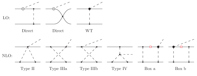
Figure 1: Complete set of diagrams up to NLO (in the $\Delta$-less theory). Solid (dashed) lines denote nucleons (pions). Solid dots correspond to the leading vertices from ${\cal L}^{(1)}_{\pi\!N}$ and ${\cal L}_{\pi\pi}^{(2)}$, as given in the main text, $\odot$ stands for the sub-leading vertices from ${\cal L}^{(2)}_{\pi\!N}$ whereas the blob indicates the possibility to have both leading and subleading vertices. The $NN$ contact interaction is represented by the leading S-wave LECs $C_{S}$ and $C_{T}$. The red square in the box diagrams indicates that the corresponding nucleon propagator cancels with parts of the $\pi N$ vertex and leads to the irreducible contribution, see text for further details.

The diagrams containing only pion and nucleon degrees of freedom that contribute to the reaction $NN\to NN\pi$ up to NLO in our expansion, are shown in Fig. 1. Details of the evaluations of each of the loop diagrams can be found in appendices A and B. The first two diagrams in the first line are sometimes called the “direct” one-nucleon diagrams in the literature, whereas the last (rightmost) diagram is called the rescattering diagram. We will discuss both next.

At leading order one needs to deal with the “direct” pion emission from a single nucleon where the nucleon recoil $\pi NN$ vertex of ${\cal L}^{(2)}_{\pi\!N}$ (6) is necessary in order to produce an outgoing s-wave pion. In addition, at LO there is a rescattering operator with the Weinberg–Tomozawa (WT) $\pi\pi NN$ vertex which, however, contributes only to the charged pion channel due to its isovector nature. In order to clarify the counting in MCS, we will concentrate on the first of two “direct” diagrams in Fig. 1. In this diagram each vertex attached to the pion propagator involves a momentum $p$. The pion propagator itself involves a momentum $p$, i.e. it is counted as $p^{-2}$, whereas the nucleon propagator only carries an energy $\propto m_{\pi}$. The $m_{\pi}^{-1}$ of the nucleon propagator cancels the factor $m_{\pi}$ of the s-wave pion production vertex, which counts as $\sim m_{\pi}p/m_{\!N}$. Thus, counting the “momentum flow” in the vertices and propagators of the diagram, gives an order of magnitude estimate of the direct diagrams (as well as the rescattering diagram) as $p/m_{\!N}$. These diagrams are counted as LO in MCS. Traditionally the LO direct diagrams have been evaluated numerically by including the pion propagator in the distorted $NN$ wave functions, i.e. only the one-nucleon-pion production vertex gives the transition operator. Numerically, in the traditional distorted wave Born approximation approach, the “direct” term appears to be significantly smaller than the estimate based on our naive MCS’s dimensional analysis. This suppression comes from two sources: first, there is the momentum mismatch between the initial and final distorted nucleon wave functions hanhart04 — see also Ref. BM for a more detailed discussion. Secondly, there are accidental cancellations from the final state interaction present in both channels, $pp\to pp\pi^{0}$ and $pp\to d\pi^{+}$, that are not accounted for in the power counting. Specifically, the $NN$ phase shift in the ${}^{1}S_{0}$ partial wave relevant for $pp\to pp\pi^{0}$ crosses zero at an energy close to the pion production threshold SAID . All realistic $NN$ scattering potentials that reproduce this feature show in the half-off-shell amplitude at low energies a zero at off-shell momenta of a similar magnitude. The exact position of the zero varies between different models, such that the direct production amplitude turns out to be quite model dependent. The suppression mechanism of the direct term for the reaction $pp\to d\pi^{+}$ comes from a strong cancellation between the deuteron S-wave and D-wave components. Thus, it is not surprising that numerically the “direct” terms in both channels are about an order of magnitude smaller than the LO amplitude from the rescattering diagram, which turns out to be consistent with the dimensional analysis. Since this LO contribution is forbidden by selection rules for $pp\to pp\pi^{0}$ while allowed for $pp\to d\pi^{+}$, one understands directly why a theoretical understanding is a lot more difficult to achieve for the former reaction.

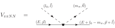
Figure 2: The $\pi N\to\pi N$ transition vertex: definition of kinematic variables as used in Eq. (8).

At NLO, which corresponds to the order $p^{2}/m_{\!N}^{2}$, loop diagrams illustrated in Fig. 1 start to contribute to the s-wave pion production amplitude. For the channel $pp\to pp\pi^{0}$ the sum of NLO diagrams type II, III and IV in Fig. 1 is zero due to a cancellation between individual diagrams HanKai . However, the same sum of diagrams II – IV gives a finite answer for the channel $pp\to d\pi^{+}$ HanKai . As a result the net contribution of these diagrams depends linearly on the $NN$ relative momentum which results in a large sensitivity to the short-distance $NN$ wave functions Gardestig . This puzzle was solved in Ref. lensky2 , where it was demonstrated that for the deuteron channel there is an additional contribution at NLO, namely the box diagrams in Fig. 1, stemming from the time-dependence of the Weinberg–Tomozawa pion-nucleon vertex. To demonstrate this, we write the expression for the WT $\pi N\to\pi N$ vertex in the notation of Fig. 2 as:

$$V_{\pi\pi NN} = l_{0}{+}m_{\pi}{-}\frac{\vec{l}\cdot(2\vec{p}+\vec{l})}{2m_{\!N}}$$ (8)

$$= {2m_{\pi}}+{\left(l_{0}{-}m_{\pi}{+}E{-}\frac{(\vec{l}+\vec{p})^{2}}{2m_{\!N}}+i0\right)}-{\left(E{-}\frac{\vec{p}\,^{2}}{2m_{\!N}}+i0\right)}\ ,$$

where we kept the leading WT vertex and its nucleon recoil correction, which are of the same order in the MCS, as explained below. For simplicity we omit the isospin dependence of the vertex. The first term in the last line is the WT-vertex for kinematics with the on-shell incoming and outgoing nucleons, the second term the inverse of the outgoing nucleon propagator while the third one is the inverse of the incoming nucleon propagator. Note that for on-shell incoming and outgoing nucleons, the expressions in brackets in (8) vanish, and the $\pi N\to\pi N$ transition vertex takes its on-shell value $2m_{\pi}$ (even if the incoming pion is off-shell). This is in contrast to standard phenomenological treatments koltunundreitan , where $l_{0}$ in the first line of (8) is identified with $m_{\pi}/2$, the energy transfer in the on-shell kinematics for $NN\to NN\pi$, but the recoil terms in Eq. (8) are not considered. However, $\vec{p}^{\ 2}/m_{\!N}\approx m_{\pi}$ so that the recoil terms are to be kept in the vertices and in the nucleon propagator. The MCS is explicitly designed to properly keep track of these recoil terms. A second consequence of Eq. (8) is that only the first term leads to a reducible diagram when the rescattering diagram with the $\pi N\to\pi N$ vertex is convoluted with $NN$ wave functions. The second and third terms in Eq. (8), however, lead to irreducible contributions, since one of the nucleon propagators is cancelled.

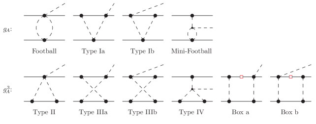
Figure 3: One-loop diagrams contributing to s-wave pion production at NLO and N²LO. Notation is as in Fig. 1.

This is illustrated by red squares on the nucleon propagators in the two box diagrams of Fig. 3. It was shown explicitly in Ref. lensky2 that those induced irreducible contributions cancel exactly the finite remainder of the NLO loops (II – IV) in the $pp\to d\pi^{+}$ channel. As a consequence, there are no contributions at NLO for both $\pi^{0}$ and $\pi^{+}$ productions, see also our results in the two first rows of Tables 1 and 2.

In this paper we extend the analysis of the previous studies and evaluate the contribution from pion loops at N²LO. Once the complete calculation at N²LO is performed, the calculated theoretical uncertainty based on our power counting is going to be reduced to $\sim(m_{\pi}/m_{\!N})^{3/2}<10\%$ for the amplitudes. At N²LO, one gets contributions from two sets of loop diagrams which differ in the power of $g_{A}$. The diagrams proportional to $g_{A}^{3}$ are the subleading contributions to the NLO diagrams of Fig. 1 we already discussed. In addition, there is a set of pion loop diagrams proportional to $g_{A}$, see Fig. 3. A naive MCS estimates indicate that the diagrams proportional to $g_{A}$ could play a role already at NLO. However, a more careful analysis reveals that the contributions of each of these $g_{A}$ diagrams at NLO is zero, see Appendix B.1 for a detailed discussion. In subsequent sections it will be shown that partial cancellations take place among $g_{A}$ and $g_{A}^{3}$ diagrams at N²LO. Unlike the cancellation among the $g_{A}^{3}$ diagrams at NLO, the cancellations at N²LO are not complete so that there is a non-zero transition amplitude from the $g_{A}$ and $g_{A}^{3}$ diagrams.

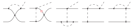
Figure 4: Exemplary irreducible diagrams that contribute at higher than N²LO. Notation is as in Fig. 1.

We already discussed pion loop diagrams with the $\pi N\to\pi N$ vertex stemming from the leading Weinberg–Tomozawa term, ${\cal L}^{(1)}_{\pi\!N}$, and its recoil correction, ${\cal L}^{(2)}_{\pi\!N}$. In addition, there are two kinds of loop diagrams in Fig. 3 which involve the $c_{i}$-vertices from ${\cal L}^{(2)}_{\pi\!N}$: those where the $c_{i}$ terms appear at the vertex, where the outgoing on-shell pion is emitted, and those where they provide an intermediate interaction. The former kind appears to be suppressed for s-wave pion production due to the pion kinematics near threshold. The Lagrangian term containing $c_{4}$ can not contribute at an outgoing s-wave pion vertex since it is proportional to the gradient of the pion fields, cf. Eq. (6). The contribution of the $c_{3}$ Lagrangian term via this type of vertex is only non-zero if the term proportional to the time derivative of the pion field is considered in the Lagrangian, cf. Eq. (6). This $c_{3}$ term, however, results in a loop amplitude which is suppressed by $m_{\pi}/m_{\!N}$ compared to the leading loop at NLO, and thus it is of higher order (N³LO). In addition, the contributions proportional to LECs $c_{1}$ and $c_{2}$ are quadratic with $m_{\pi}$ and therefore strongly suppressed. However, the contributions of the vertices proportional to $c_{2}$, $c_{3}$ and $c_{4}$ are potentially important at N²LO once embedded in the off-shell intermediate $\pi N$ vertices (on the lower nucleon line of the $g_{A}$-type diagrams in Fig. 3). In what follows we will discuss the individual contributions of loops in detail.

As a final remark, we give in Fig. 4 some examples of additional loop topologies which start to contribute at a higher order than what is considered in the present study. The common feature of these diagrams is the presence of only one pion propagator inside the loops. As a consequence, by using appropriate integration variables, one can eliminate the large initial three-momentum $\vec{p}$ from the loop integrals, meaning the loop momentum will scale with $m_{\pi}$. This explains why these loop diagrams in Fig. 4 only start to contribute at order N³LO or higher.

III Calculation of diagrams proportional to $g_{\!A}^{3}$

The diagrams of the $g_{\!A}^{3}$-group in Fig. 3 have a common structure illustrated in Fig. 5.

Figure 5: The general structure of $g_{\!A}^{3}$ diagrams.

The loop diagram in Fig. 5 is integrated over the momentum $l=(l_{0},\vec{l})$. We also use the short-hand notation

$$\tilde{l}=l+k_{1}-q\;,$$

with $k_{1}=p_{1}-p_{1}^{\prime}$. The pion isospin indices $a$, $b$, and $c$ are defined as shown in Fig. 5. The circle containing the vertex operator $A^{abc}$ produces an outgoing pion of isospin index $a$ off nucleon 1. This operator is different for each diagram and its explicit form is derived in Appendix A, where also the detailed structure of each $g_{A}^{3}$-diagram is given.

The invariant amplitude for each relevant diagram proportional to $g_{A}^{3}$ can be written as

$$iM_{g_{\!A}^{3}}=\int\!\!\!\frac{d^{4}l}{(2\pi)^{4}}\,B_{2}(l,\tilde{l})\ \tau_{2}^{c}\tau_{2}^{b}\ A_{g_{\!A}^{3}}^{abc},$$ (9)

where $B_{2}(l,\tilde{l})$ is the common operator structure associated with nucleon 2 in Fig. 5. The operator $B_{2}(l,\tilde{l})$ involves two pion propagators, two $\pi NN$-vertices and the nucleon propagator. The explicit form of $B_{2}(l,\tilde{l})$ can be read off from the diagram in Fig. 5:

$$B_{2}(l,\tilde{l}) = \frac{i}{l^{2}-m_{\pi}^{2}+i0}\;\frac{i}{\tilde{l}^{2}-m_{\pi}^{2}+i0}\;\frac{i}{p_{20}-l_{0}-\frac{(\vec{p}_{2}-\vec{l})^{2}}{2m_{\!N}}+i0}$$ (10)

$$\times\frac{g_{\!A}}{f_{\!\pi}}\left(-S_{2}\cdot\tilde{l}+\frac{S_{2}\cdot(p_{2}+p_{2}^{\,\prime}-l)v\cdot\tilde{l}}{2m_{\!N}}\right)$$

$$\times\frac{g_{\!A}}{f_{\!\pi}}\left(S_{2}\cdot l-\frac{S_{2}\cdot(2p_{2}-l)v\cdot l}{2m_{\!N}}\right),$$

where $v^{\mu}=(1,\vec{0})$ is the nucleon four-velocity and $S^{\mu}=(0,{\vec{\sigma}}/2)$ is its spin-vector. Note that $B_{2}(l,\tilde{l})$ contains no isospin indices as all isospin operators are included in Eq. (9). Since the structure of $B_{2}(l,\tilde{l})$ is the same for all considered $g_{A}^{3}$ diagrams we will consider, we concentrate our discussion on the structure of operator $A_{g_{\!A}^{3}}^{abc}$ in Eq. (9), see Appendix A for details. Note that the amplitude, Eq. (9) is not yet properly symmetrized with respect to the two nucleons. Below we will first discuss, how the partial cancellation amongst the various pion loop diagrams emerges on the basis of the decomposition illustrated in Fig. 5. In Sec. V the non-vanishing remainder will be given in a symmetrized form.

III.1 Pion s-wave contributions $\propto g_{\!A}^{3}$

In Appendix A we derive the expressions for each of the six $g_{A}^{3}$ diagrams which contribute to near-threshold s-wave pion production from two nucleons. The results of these calculations are summarized in Table 1 where, for convenience, we have introduced the following short-hand notation for the isospin structures:

$$\tau_{\!+}=(\bm{\tau}_{1}+\bm{\tau}_{2})^{a},\qquad\tau_{\!-}=(\bm{\tau}_{1}-\bm{\tau}_{2})^{a},\qquad\tau_{\!\times}=i(\bm{\tau}_{1}\times\bm{\tau}_{2})^{a}.$$ (11)

The left column in Table 1 shows the spin structures that emerge in these diagrams, the next six columns represent the contributions from the individual diagrams to the given spin structure, whereas the last two columns summarize the net effect of all diagrams and the MCS order, respectively. When we add the resulting expressions for the six diagrams we confirm the finding of Ref. lensky2 that the sum of the NLO contributions from all diagrams vanishes, see the first two rows of operators in Table 1. Moreover, since the sum of the operators in the first two rows of Table 1 is an exact zero, the corresponding spin-momentum structures $S_{1}\cdot l$ and $S_{1}\cdot\tilde{l}$ will not contribute also at N²LO and all higher orders. In addition, all nucleon recoil corrections $\propto 1/(2m_{\!N})$ to the individual diagrams at N²LO also cancel in the sum. The reason for that cancellation is completely analogous to the cancellation that happens at NLO, see discussion below Eq. (8). In fact, only those parts of the $g_{A}^{3}$ diagrams that cannot be reduced to the topology of the diagram II in Fig. 3, give a non-zero contribution to the transition amplitude. Thus, only very few N²LO contributions to the pion production amplitude remain, as seen in Table 1. The non-vanishing terms appear from the two cross-box diagrams and diagram IV.

Since the sum of the $A_{g_{\!A}^{3}}^{abc}$ operators from the different diagrams starts to contribute at N²LO, we keep only the leading part of the operator $B_{2}(l,\tilde{l})$. Adding up the contributions from all six $g_{A}^{3}$ diagrams we arrive at the following result:

$$iM^{\text{N${}^{2}$LO{}}}_{g_{\!A}^{3}} = i\frac{g_{\!A}^{3}}{4f_{\!\pi}^{5}}\int\!\!\!\frac{d^{4}l}{(2\pi)^{4}}\,\frac{S_{2}\cdot\tilde{l}}{l^{2}-m_{\pi}^{2}+i0}\;\frac{S_{2}\cdot l}{\tilde{l}^{2}-m_{\pi}^{2}+i0}\;\frac{1}{-v\cdot l+i0}$$ (12)

$$\times\biggl{\{}(-2\tau_{\!+}+\tau_{\!\times})\frac{2v\cdot q}{-v\cdot l+i0}(S_{1}\cdot\tilde{l})+(-2\tau_{\!+}-\tau_{\!\times})\frac{2v\cdot q}{-v\cdot l+i0}(S_{1}\cdot l)$$

$$-8\tau_{\!\times}(S_{1}\cdot k_{1})\frac{(l+\tilde{l})\cdot q}{k_{1}^{2}-m_{\pi}^{2}+i0}\biggr{\}},$$

where for the nucleon propagator in Eq. (10) we dropped $p_{20}$ and all recoil terms of order ${\cal O}(m_{\pi})$ compared to the lower-order $l_{0}\equiv v\cdot l\sim|\vec{l}|\sim p$ term. Rearranging the isospin structure we arrive at three independent integrals to be evaluated for s-wave pion production:

$$iM^{\text{N${}^{2}$LO{}}}_{g_{\!A}^{3}} = -i\frac{g_{\!A}^{3}}{4f_{\!\pi}^{5}}\biggl{\{}4(v\cdot q)\tau_{\!+}S_{2}^{\mu}S_{2}^{\nu}S_{1}^{\lambda}\int\limits\frac{d^{4}l}{(2\pi)^{4}}\frac{\tilde{l}_{\mu}l_{\nu}(l+\tilde{l})_{\lambda}}{(l^{2}-m_{\pi}^{2}+i0)(\tilde{l}^{2}-m_{\pi}^{2}+i0)(-v\cdot l+i0)^{2}}$$ (13)

$$-2(v\cdot q)\tau_{\!\times}S_{2}^{\mu}S_{2}^{\nu}(S_{1}\cdot k_{1})\int\limits\frac{d^{4}l}{(2\pi)^{4}}\frac{\tilde{l}_{\mu}l_{\nu}}{(l^{2}-m_{\pi}^{2}+i0)(\tilde{l}^{2}-m_{\pi}^{2}+i0)(-v\cdot l+i0)^{2}}$$

$$+8q^{\lambda}\tau_{\!\times}\frac{S_{2}^{\mu}S_{2}^{\nu}(S_{1}\cdot k_{1})}{k_{1}^{2}-m_{\pi}^{2}+i0}\int\limits\frac{d^{4}l}{(2\pi)^{4}}\frac{\tilde{l}_{\mu}l_{\nu}(l+\tilde{l})_{\lambda}}{(l^{2}-m_{\pi}^{2}+i0)(\tilde{l}^{2}-m_{\pi}^{2}+i0)(-v\cdot l+i0)}\biggr{\}}$$

Table 1: Interference pattern of NLO and N²LO s-wave contributions from the individual $g_{\!A}^{3}$ diagrams. The Table shows the contributions to the vertex $\tau_{2}^{c}\tau_{2}^{b}\ A_{g_{\!A}^{3}}^{abc}$ defined in Eq.(9) and Fig. 5. These contributions are given separately for the different spin-momentum structures of the vertex $A_{g_{\!A}^{3}}^{abc}$, shown in the leftmost column. The notation for the isospin structures is defined in Eq.(11).

	Type II	Type IIIa	Type IIIb	Type IV	Box a	Box b	Sum	Order
$S_{1}\cdot l$	$-4\tau_{\!+}-4\tau_{\!-}+2\tau_{\!\times}$	$0$	$-2\tau_{\!+}-\tau_{\!\times}$	$\phantom{+}6\tau_{\!+}+6\tau_{\!-}$	$-2\tau_{\!-}-\tau_{\!\times}$	$0$	$0$	NLO, N2LO
$S_{1}\cdot\tilde{l}$	$\phantom{+}4\tau_{\!+}+4\tau_{\!-}+2\tau_{\!\times}$	$\phantom{+}2\tau_{\!+}-\tau_{\!\times}$	$0$	$-6\tau_{\!+}-6\tau_{\!-}$	$0$	$\phantom{+}2\tau_{\!-}-\tau_{\!\times}$	$0$	NLO, N2LO
$S_{1}\cdot l\,\frac{v\cdot\tilde{l}}{2m_{\!N}}$	$-2\tau_{\!+}+2\tau_{\!-}$	$\phantom{+}2\tau_{\!+}-\tau_{\!\times}$	$0$	$0$	$0$	$-2\tau_{\!-}+\tau_{\!\times}$	$0$	N2LO
$S_{1}\cdot\tilde{l}\,\frac{v\cdot l}{2m_{\!N}}$	$\phantom{+}2\tau_{\!+}-2\tau_{\!-}$	$0$	$-2\tau_{\!+}-\tau_{\!\times}$	$0$	$\phantom{+}2\tau_{\!-}+\tau_{\!\times}$	$0$	$0$	N2LO
$S_{1}\cdot(p_{1}{+}p_{1}^{\,\prime})\,\frac{v\cdot l}{2m_{\!N}}$	$\phantom{+}4\tau_{\!+}+4\tau_{\!-}-2\tau_{\!\times}$	$0$	$\phantom{+}2\tau_{\!+}+\tau_{\!\times}$	$-6\tau_{\!+}-6\tau_{\!-}$	$\phantom{+}2\tau_{\!-}+\tau_{\!\times}$	$0$	$0$	N2LO
$S_{1}\cdot(p_{1}{+}p_{1}^{\,\prime})\,\frac{v\cdot\tilde{l}}{2m_{\!N}}$	$-4\tau_{\!+}-4\tau_{\!-}-2\tau_{\!\times}$	$-2\tau_{\!+}+\tau_{\!\times}$	$0$	$\phantom{+}6\tau_{\!+}+6\tau_{\!-}$	$0$	$-2\tau_{\!-}+\tau_{\!\times}$	$0$	N2LO
$S_{1}\cdot l\frac{2v\cdot q}{-v\cdot l+i0}$	$0$	$0$	$-2\tau_{\!+}-\tau_{\!\times}$	$0$	$0$	$0$	$-2\tau_{\!+}-\tau_{\!\times}$	N2LO
$S_{1}\cdot\tilde{l}\frac{2v\cdot q}{-v\cdot l+i0}$	$0$	$-2\tau_{\!+}+\tau_{\!\times}$	$0$	$0$	$0$	$0$	$-2\tau_{\!+}+\tau_{\!\times}$	N2LO
$S_{1}\cdot k_{1}\frac{q\cdot(l+\tilde{l})}{k_{1}^{2}-m_{\pi}^{2}+i0}$	$0$	$0$	$0$	$-8\tau_{\!\times}$	$0$	$0$	$-8\tau_{\!\times}$	N2LO

Employing dimensional regularization and an integration method outlined in Appendix C, Eq. (13) can be brought into the more transparent form:

$$iM^{\text{N${}^{2}$LO{}}}_{g_{\!A}^{3}} = \frac{g_{\!A}^{3}(v\cdot q)}{f_{\!\pi}^{5}}\bigg{\{}\tau_{\!+}i\varepsilon^{\mu\nu\alpha\beta}k_{1\mu}S_{1\nu}v_{\alpha}S_{2\beta}\left[-J(k_{1}^{2})\right]$$ (14)

$$+\tau_{\!\times}(S_{1}\cdot k_{1})\left[-\frac{19}{24}J(k_{1}^{2})+\frac{5}{9}\frac{1}{(4\pi)^{2}}\right]\bigg{\}},$$

where we have only kept the lowest order parts of the integrals which give contributions to the amplitude at N²LO. The pion loop diagrams generate ultraviolet divergent terms, which are contained in the following integral:

$$J(k_{1}^{2})=-i\int\limits\frac{d^{4}l}{(2\pi)^{4}}\frac{1}{l^{2}-m_{\pi}^{2}+i0}\frac{1}{(l+k_{1})^{2}-m_{\pi}^{2}+i0}$$ (15)

The divergences are to be absorbed by the LECs accompanying the five-point ($4N\pi$) vertices as we will discuss in Sec. VI.

IV Calculation of diagrams proportional to $g_{\!A}$

We evaluate the $g_{\!A}$ diagrams following a similar strategy we used when we evaluated the $g_{\!A}^{3}$ diagrams. The invariant amplitude for each diagram proportional to $g_{A}$ can be written as

$$iM_{g_{\!A}}=\int\!\!\!\frac{d^{4}l}{(2\pi)^{4}}\,D_{2}(l,\tilde{l})\ \varepsilon^{bcd}\tau_{2}^{d}\ A_{g_{\!A}}^{abc},$$ (16)

where $D_{2}(l,\tilde{l})$ is a common operator structure which is associated with nucleon 2 in Fig. 6.

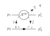
Figure 6: The general structure of $g_{\!A}$ diagrams.

This structure involves the WT vertex at the second nucleon and the two pion propagators:

$$D_{2}(l,\tilde{l})=\frac{i}{l^{2}-m_{\pi}^{2}+i0}\;\frac{i}{\tilde{l}^{2}-m_{\pi}^{2}+i0}\;\frac{v\cdot(l+\tilde{l})}{4f_{\!\pi}^{2}}.$$ (17)

Note that we have only written the leading WT-vertex contribution in $D_{2}(l,\tilde{l})$, Eq. (17), since the sum of the $A_{g_{A}}^{abc}$ operators starts to contribute at N²LO only, as can be seen in Table 2. This is in full analogy to the sum of the $A_{g_{A}^{3}}^{abc}$ operators, which also only start to contribute at N²LO, where, as discussed just before Eq. (12), the recoil ($1/m_{N}$) corrections in $B_{2}(l,\tilde{l})$, Eq. (10), only contribute at higher order. In other words, the corrections to $D_{2}(l,\tilde{l})$, that is the recoil correction to the leading WT interaction term and the correction stemming from the $c_{4}$-vertex, contribute at a higher order than what is considered in this work. Notice further that the $c_{2}$ and $c_{3}$-vertices in Eq. (6) are isoscalars and, therefore, do not contribute to the function $D_{2}(l,\tilde{l})$. The contributions of these LECs will be discussed in the next section.

IV.1 Pion s-wave contributions $\propto g_{\!A}$

The operator expressions for each individual diagram of the $g_{A}$-type contributing to s-wave pion production can be found in Appendix B. In a complete analogy with the $g_{A}^{3}$ diagrams, we summarize in Table 2 the contributions of the individual diagrams and their net effect for different spin structures. In distinction to the $g_{A}^{3}$-graphs the diagrams of this topology do not appear, contrary to naive MCS expectations, at NLO, see Appendix B.1 for a more detailed discussion. Similarly to $g_{A}^{3}$-type contributions, only a few of the N²LO terms do not cancel in the sum. Again, only those parts of the diagrams Ia, Ib and mini-football that cannot be reduced to the topology of the football diagram in Fig. 3, give a non-zero contribution to the transition amplitude. The results are shown in Table 2, and the sum of these $g_{A}$ contributions gives the following transition amplitude:

$$iM^{\text{N${}^{2}$LO{}}}_{g_{\!A}} = i\frac{g_{\!A}}{8f_{\!\pi}^{3}}\int\!\!\!\frac{d^{4}l}{(2\pi)^{4}}\,D_{2}(l,\tilde{l})\ \biggl{\{}(2\tau_{\!+}-2\tau_{\!-}-2\tau_{\!\times})\frac{2v\cdot q}{-v\cdot l+i0}S_{1}\cdot\tilde{l}$$ (18)

$$+(2\tau_{\!+}-2\tau_{\!-}+2\tau_{\!\times})\frac{2v\cdot q}{-v\cdot l+i0}S_{1}\cdot l+8\tau_{\!\times}\;S_{1}\cdot k_{1}\frac{q\cdot(l+\tilde{l})}{k_{1}^{2}-m_{\pi}^{2}+i0}\biggr{\}}.$$

Table 2: Interference pattern of s-wave contributions from the individual $g_{\!A}$ diagrams. The Table shows the contributions to the vertex $\varepsilon^{bcd}\tau_{2}^{d}A_{g_{\!A}}^{abc}$ defined in Fig. 6 and Eq.(16). The contributions are given separately for different spin-momentum structures of the vertex $A_{g_{\!A}}^{abc}$, shown in the leftmost column. The notation for the isospin structures is defined in Eq.(11).

	Football	Type Ia	Type Ib	MiniFB	Sum	Order
$S_{1}\cdot l$	$-2\tau_{\!\times}$	$-\tau_{\!+}+\tau_{\!-}+\tau_{\!\times}$	$\phantom{+}\tau_{\!+}-\tau_{\!-}+\tau_{\!\times}$	$0$	$0$	NLO, N2LO
$S_{1}\cdot\tilde{l}$	$-2\tau_{\!\times}$	$-\tau_{\!+}+\tau_{\!-}+\tau_{\!\times}$	$\phantom{+}\tau_{\!+}-\tau_{\!-}+\tau_{\!\times}$	$0$	$0$	NLO, N2LO
$S_{1}\cdot l\,\frac{v\cdot\tilde{l}}{2m_{\!N}}$	$\phantom{+}2\tau_{\!+}-2\tau_{\!-}$	$-\tau_{\!+}+\tau_{\!-}+\tau_{\!\times}$	$-\tau_{\!+}+\tau_{\!-}-\tau_{\!\times}$	$0$	$0$	N2LO
$S_{1}\cdot\tilde{l}\,\frac{v\cdot l}{2m_{\!N}}$	$-2\tau_{\!+}+2\tau_{\!-}$	$\phantom{+}\tau_{\!+}-\tau_{\!-}-\tau_{\!\times}$	$\phantom{+}\tau_{\!+}-\tau_{\!-}+\tau_{\!\times}$	$0$	$0$	N2LO
$S_{1}\cdot(p_{1}{+}p_{1}^{\,\prime})\,\frac{v\cdot l}{2m_{\!N}}$	$\phantom{+}2\tau_{\!\times}$	$\phantom{+}\tau_{\!+}-\tau_{\!-}-\tau_{\!\times}$	$-\tau_{\!+}+\tau_{\!-}-\tau_{\!\times}$	$0$	$0$	N2LO
$S_{1}\cdot(p_{1}{+}p_{1}^{\,\prime})\,\frac{v\cdot\tilde{l}}{2m_{\!N}}$	$\phantom{+}2\tau_{\!\times}$	$\phantom{+}\tau_{\!+}-\tau_{\!-}-\tau_{\!\times}$	$-\tau_{\!+}+\tau_{\!-}-\tau_{\!\times}$	$0$	$0$	N2LO
$S_{1}\cdot l\frac{2v\cdot q}{-v\cdot l+i0}$	$\phantom{+}0$	$0$	$2\tau_{\!+}-2\tau_{\!-}+2\tau_{\!\times}$	$0$	$2\tau_{\!+}-2\tau_{\!-}+2\tau_{\!\times}$	N2LO
$S_{1}\cdot\tilde{l}\frac{2v\cdot q}{-v\cdot l+i0}$	$\phantom{+}0$	$2\tau_{\!+}-2\tau_{\!-}-2\tau_{\!\times}$	$0$	$0$	$2\tau_{\!+}-2\tau_{\!-}-2\tau_{\!\times}$	N2LO
$S_{1}\cdot k_{1}\frac{q\cdot(l+\tilde{l})}{k_{1}^{2}-m_{\pi}^{2}+i0}$	$\phantom{+}0$	$0$	$0$	$8\tau_{\!\times}$	$8\tau_{\!\times}$	N2LO

We now turn to the contribution emerging from the diagrams of Fig. 3 with the $c_{2}$ and $c_{3}$-vertices in the off-shell pion kinematics at nucleon 2. We obtain the following expression for the amplitude:

$$iM^{\text{N${}^{2}$LO{}}}_{g_{\!A},c_{i}} = -i\frac{g_{\!A}}{2f_{\!\pi}^{5}}(\tau_{\!+}+\tau_{\!-})(S\cdot k_{1})$$ (19)

$$\times \int\!\!\!\frac{d^{4}l}{(2\pi)^{4}}\,\frac{c_{3}(l\cdot\tilde{l})+(c_{2}-g_{A}^{2}/8m_{N})(v\cdot l)(v\cdot\tilde{l})}{(l^{2}-m_{\pi}^{2}+i0)(\tilde{l}^{2}-m_{\pi}^{2}+i0)}\;\;\biggl{\{}2+\frac{1}{2}+\frac{1}{2}-3\biggr{\}}=0\;,$$

where the numbers in the curly bracket correspond to the individual contributions of the $g_{A}$-diagrams, as they appear in Fig. 3, in order. Again, while the individual diagrams do contribute at N²LO, their sum turns out to yield a vanishing result. We, therefore, conclude that there are no loop amplitudes $\propto c_{i}$ to the order we are working.

Upon performing some simplifications, the total result for the $g_{A}$-contribution to the transition amplitude in Eq. (18) can be brought into the form

$$iM^{\text{N${}^{2}$LO{}}}_{g_{\!A}} = -i\frac{g_{\!A}}{8f_{\!\pi}^{5}}\biggl{\{}(\tau_{\!+}-\tau_{\!-})(v\cdot q)\int\!\!\!\frac{d^{4}l}{(2\pi)^{4}}\,\frac{v\cdot(l+\tilde{l})S_{1}\cdot(l+\tilde{l})}{(l^{2}-m_{\pi}^{2}+i0)(\tilde{l}^{2}-m_{\pi}^{2}+i0)(-v\cdot l+i0)}$$ (20)

$$-\tau_{\!\times}(v\cdot q)(S_{1}\cdot k_{1})\int\!\!\!\frac{d^{4}l}{(2\pi)^{4}}\,\frac{v\cdot(l+\tilde{l})}{(l^{2}-m_{\pi}^{2}+i0)(\tilde{l}^{2}-m_{\pi}^{2}+i0)(-v\cdot l+i0)}$$

$$+2\tau_{\!\times}(S_{1}\cdot k_{1})\frac{1}{k_{1}^{2}-m_{\pi}^{2}+i0}\int\!\!\!\frac{d^{4}l}{(2\pi)^{4}}\,\frac{v\cdot(l+\tilde{l})q\cdot(l+\tilde{l})}{(l^{2}-m_{\pi}^{2}+i0)(\tilde{l}^{2}-m_{\pi}^{2}+i0)}\biggr{\}}\,.$$

The first term in Eq. (20) does not contribute at N²LO, since at this order the term $v\cdot(l+\tilde{l})\approx 2v\cdot l$ in the numerator cancels with the nucleon propagator $-v\cdot l+i0$. The resulting integral vanishes due to the symmetry of the integrand. Specifically, the integral is to be invariant under the shift of variables ($l\to-\tilde{l},\tilde{l}\to-l$). Indeed, the denominator of this integrand is invariant under this transformation whereas the numerator changes its sign. Therefore, the first term in Eq. (20) is equal to zero. Finally, keeping only the lowest-order terms as appropriate at N²LO and using the expressions for the loop integrals outlined in Appendix C, we arrive at the final result:

$$iM^{\text{N${}^{2}$LO{}}}_{g_{\!A}}=\frac{g_{\!A}}{f_{\!\pi}^{5}}\tau_{\!\times}(v\cdot q)(S_{1}\cdot k_{1})\left[\frac{1}{6}J(k_{1}^{2})-\frac{1}{18}\frac{1}{(4\pi)^{2}}\right]\,,$$ (21)

where the UV-divergent integral $J(k_{1}^{2})$ is defined in Eq. (15).

V Summary of the two-pion exchange diagrams

Until now we have evaluated the expressions for the production operator assuming that the pion is produced from nucleon 1. We now add the contribution emerging from interchanging the nucleon labels. We use the fact that in the center-of-mass system $\vec{p}_{1}=-\vec{p}_{2}=\vec{p}$ and $k_{1}=-k_{2}+q$ and employ the approximate relation $k_{1}^{2}\simeq k_{2}^{2}$ with higher-order terms being ignored. Throughout, we also ignore operators leading to pion p-wave production. We then obtain from Eqs. (21) and (14) the following complete (i.e. symmetrized with respect to the nucleon labels) expressions:

$$iM^{\text{N${}^{2}$LO{}}}_{g_{\!A}}=\frac{g_{\!A}\ (v\cdot q)}{f_{\!\pi}^{5}}\tau_{\!\times}(S_{1}+S_{2})\cdot k_{1}\left[\frac{1}{6}J(k_{1}^{2})-\frac{1}{18}\frac{1}{(4\pi)^{2}}\right]\;,$$ (22)

$$iM^{\text{N${}^{2}$LO{}}}_{g_{\!A}^{3}} = \frac{g_{\!A}^{3}\ (v\cdot q)}{f_{\!\pi}^{5}}\bigg{\{}\tau_{\!+}i\varepsilon^{\alpha\mu\nu\beta}v_{\alpha}k_{1\mu}S_{1\nu}S_{2\beta}\left[-2J(k_{1}^{2})\right]$$ (23)

$$+\tau_{\!\times}(S_{1}+S_{2})\cdot k_{1}\left[-\frac{19}{24}J(k_{1}^{2})+\frac{5}{9}\frac{1}{(4\pi)^{2}}\right]\bigg{\}}.$$

Employing dimensional regularization, $d=4-\varepsilon$), the integral $J(k_{1})$ entering the above expressions can be written in the form

$$J(k_{1}^{2}) = \frac{\mu^{\varepsilon}}{i}\int\frac{d^{(4-\varepsilon)}l}{(2\pi)^{(4-\varepsilon)}}\frac{1}{[l^{2}-m_{\pi}^{2}+i0][(l+k_{1})^{2}-m_{\pi}^{2}+i0]}$$ (24)

$$= -2L-\frac{1}{(4\pi)^{2}}\left[\log\left(\frac{m_{\pi}^{2}}{\mu^{2}}\right)-1+2F_{1}\left(\frac{k_{1}^{2}}{m_{\pi}^{2}}\right)\right],$$

where the function $F_{1}(x)$ is defined via

$$F_{1}(x)=\frac{\sqrt{4-x-i0}}{\sqrt{x}}\arctan\left(\frac{\sqrt{x}}{\sqrt{4-x-i0}}\right)\,.$$ (25)

and the UV divergency appears as a simple pole in the function $L$:

$$L=\frac{1}{(4\pi)^{2}}\left[-\frac{1}{\varepsilon}+\frac{1}{2}\left(\gamma_{E}-1-{\log}(4\pi)\right)\right].$$ (26)

Note that both $M^{\text{N${}^{2}$LO{}}}_{g_{\!A}}$ and $M^{\text{N${}^{2}$LO{}}}_{g_{\!A}^{3}}$ are proportional to the outgoing pion energy $v\cdot q\simeq m_{\pi}$, i.e. both operator amplitudes vanish at threshold in the chiral limit.

VI Regularization procedure

In MCS the loop diagrams which contribute to the renormalization of e.g. the nucleon mass $m_{\!N}$ and the axial coupling constant $g_{A}$ do not involve large-momentum components. Consequently, these diagrams contribute in the MCS at order N⁴LO which is beyond the scope of the present work. For example, consider a LO rescattering diagram which in our naive counting is of order $\sqrt{m_{\pi}/m_{\!N}}$. Including a pion loop in any of these diagram will require a renormalization any of the vertices in these LO diagrams, cf. e.g. the last three diagrams in Fig. 4. This pion loop will increase the MCS order by factor $(m_{\pi}/m_{\!N})^{2}$ as shown in, e.g. Ref. hanhart04 , Table 11. At N²LO, we only have to consider the loop diagrams which are evaluated in this paper. The UV divergences appearing in the corresponding integrals are to be absorbed into LECs accompanying the $4N\pi$ amplitudes ${\cal A}_{\text{CT}}$ and ${\cal B}_{\text{CT}}$ introduced in Sec. II.1. The contributions of the loops to the amplitudes ${\cal A}$ and ${\cal B}$, see Eq. (3), can be separated into singular and finite parts

$${\cal A} = \frac{m_{\pi}}{(4\pi f_{\!\pi})^{2}f_{\!\pi}^{3}}(\tilde{\cal A}_{\text{singular}}+\tilde{\cal A}_{\text{finite}}),$$

$${\cal B} = \frac{m_{\pi}}{(4\pi f_{\!\pi})^{2}f_{\!\pi}^{3}}(\tilde{\cal B}_{\text{singular}}+\tilde{\cal B}_{\text{finite}}),$$ (27)

where

$$\tilde{\cal A}_{\text{singular}}=g_{A}^{3}(4\pi)^{2}L,\quad\quad\tilde{\cal B}_{\text{singular}}=-\frac{g_{A}}{6}\left(\frac{19}{4}g_{A}^{2}-1\right)(4\pi)^{2}L\;.$$ (28)

Here we have used that at threshold $\vec{k}_{1}=\vec{p}$ and $v\cdot q=m_{\pi}$. Notice that the above decomposition into singular and finite pieces is, clearly, scheme dependent. Analogously, the amplitudes given by the $4N\pi$ Lagrangian contact terms, which are given in, e.g., Ref. cohen , are written as:

$${\cal A}_{\text{CT}}=\frac{m_{\pi}}{(4\pi f_{\!\pi})^{2}f_{\!\pi}^{3}}(\tilde{\cal A}^{r}_{\text{CT}}(\mu)+(4\pi)^{2}\beta_{\cal A}L),\quad{\cal B}_{\text{CT}}=\frac{m_{\pi}}{(4\pi f_{\!\pi})^{2}f_{\!\pi}^{3}}(\tilde{\cal B}^{r}_{\text{CT}}(\mu)+(4\pi)^{2}\beta_{\cal B}L)\;.$$ (29)

The singular parts of the amplitudes in Eq. (29) cancel the singularities of the amplitudes in Eq. (27), emerging from the loops. The resulting finite expressions for the scattering amplitudes are given in terms of the renormalized LECs of Ref. cohen .

$${\cal A}^{r}_{\text{CT}} = \frac{m_{\pi}}{(4\pi f_{\!\pi})^{2}f_{\!\pi}^{3}}\tilde{\cal A}^{r}_{\text{CT}}=-(d_{1}^{\prime}+2e_{1}-2e_{2})\frac{m_{\pi}}{4m_{N}f_{\!\pi}}$$

$${\cal B}^{r}_{\text{CT}} = \frac{m_{\pi}}{(4\pi f_{\!\pi})^{2}f_{\!\pi}^{3}}\tilde{\cal B}^{r}_{\text{CT}}=-(d_{1}^{\prime}+2e_{1})\frac{m_{\pi}}{4m_{N}f_{\!\pi}}$$ (30)

The magnitudes of the amplitudes ${\cal A}^{r}_{\text{CT}}$ and ${\cal B}^{r}_{\text{CT}}$ can be estimated using the values of the LECs determined in Refs. cohen ; rocha ; vmr96 where the short-ranged production mechanisms were assumed to originate from z-diagrams with $\sigma$ and $\omega$ exchanges (see explicit expressions for these exchanges in Refs. cohen ; ksmk09 ). Given the estimates in Ref. vmr96 , we find $d_{1}^{\prime}+2e_{1}-2e_{2}\simeq-7.5/f^{2}_{\pi}m_{\!N}$ and $d_{1}^{\prime}+2e_{1}\simeq-3.5/f^{2}_{\pi}m_{\!N}$, and using $m_{N}\simeq 4\pi f_{\pi}$, we obtain ${\cal A}^{r}_{\text{CT}}\simeq 2\,{m_{\pi}}/{(m_{N}^{2}f_{\!\pi}^{3})}$ and ${\cal B}^{r}_{\text{CT}}\simeq 1\,{m_{\pi}}/{(m_{N}^{2}f_{\!\pi}^{3})}$, which results in $\tilde{\cal A}^{r}_{\text{CT}}\simeq 2$ and $\tilde{\cal B}^{r}_{\text{CT}}\simeq 1$.

We take these numbers to set the scale for typical N²LO contributions. Therefore, these estimates allow us to infer the importance of the pion–nucleon loop contributions to the $NN\to NN\pi$ reactions at threshold. In particular, we can compare this estimate with the finite parts of the loops given by Eqs. (22) and (23) (where $v\cdot p\sim m_{\pi}\ll|\vec{p}|$).

$$\tilde{\cal A}_{\text{finite}} = -\frac{g_{A}^{3}}{2}\left[1-\log\left(\frac{m_{\pi}^{2}}{\mu^{2}}\right)-2F_{1}\left(\frac{-{\vec{p}\,}^{2}}{m_{\pi}^{2}}\right)\right],$$

$$\tilde{\cal B}_{\text{finite}} = -\frac{g_{A}}{6}\left[-\frac{1}{2}\left(\frac{19}{4}g_{A}^{2}-1\right)\left(1-\log\left(\frac{m_{\pi}^{2}}{\mu^{2}}\right)-2F_{1}\left(\frac{-{\vec{p}\,}^{2}}{m_{\pi}^{2}}\right)\right)+\frac{5}{3}g_{A}^{2}-\frac{1}{6}\right]\ ,$$ (31)

Choosing $\mu=4\pi f_{\!\pi}$ with $f_{\!\pi}=92.4$ MeV and $g_{A}=1.32$, we find $\tilde{\cal A}_{\text{finite}}=-2.9$ and $\tilde{\cal B}_{\text{finite}}=1.4$. We, therefore, conclude that contributions of the finite parts of the loops are comparable in size with $\tilde{\cal A}^{r}_{\text{CT}}$ and $\tilde{\cal B}^{r}_{\text{CT}}$. This confirms our power counting and shows that pion loops contributions, not considered in previous analyses, are indeed significant. One should, however, keep in mind that this result was obtained for the particular regularization scheme as explained above. In general, the finite parts of the loops $\tilde{\cal A}_{\text{finite}}$ and $\tilde{\cal B}_{\text{finite}}$ can be further decomposed into the short- and long-range parts. The former one is just a (renormalization scheme dependent) constant to which all terms in Eq. (VI) but $F_{1}$ contributes. On the other hand, the long-range part of the loops is scheme-independent. By expanding the function $F_{1}(-{\vec{p}\,}^{2}/m_{\pi}^{2})$, Eq. (25), which is the only long-range piece in (VI), in the kinematical regime relevant for pion production, i.e. $({\vec{p}\,}^{2}/m_{\pi}^{2})\gg 1$, up to the terms at N²LO one obtains

$$\tilde{\cal A}^{\text{long}}_{\text{finite}} = -\frac{g_{A}^{3}}{2}\log\left(\frac{m_{\pi}^{2}}{{\vec{p}\,}^{2}}\right)+{\cal O}\left(\frac{m_{\pi}^{2}}{{\vec{p}\,}^{2}}\right),$$

$$\tilde{\cal B}^{\text{long}}_{\text{finite}} = \frac{g_{A}}{12}\left(\frac{19}{4}g_{A}^{2}-1\right)\log\left(\frac{m_{\pi}^{2}}{{\vec{p}\,}^{2}}\right)+{\cal O}\left(\frac{m_{\pi}^{2}}{{\vec{p}\,}^{2}}\right).$$ (32)

Numerical evaluation of these terms gives $\tilde{\cal A}^{\text{long}}_{\text{finite}}=2.2$ and $\tilde{\cal B}^{\text{long}}_{\text{finite}}=-1.5$. The scheme-independent long range part of N²LO pion loops appears to be as large as the resulting short-range amplitudes, $\tilde{\cal A}^{r}_{\text{CT}}$ and $\tilde{\cal B}^{r}_{\text{CT}}$, which are given by the meson-exchange mechanism, proposed in Refs. Lee ; HGM ; Hpipl ; jounicomment to resolve the discrepancy between phenomenological calculations and experimental data. Hence, the importance of the N²LO pion loop effects, not included in the previous studies, raises serious doubts on the physics interpretation behind the phenomenologically successful models of Refs. Lee ; HGM ; Hpipl ; jounicomment .

In a subsequent work we will present results for N²LO loops including the Delta resonance as well as the convolution with proper nuclear wave functions. At that point a fit to the pion production data is possible and we can extract the strength of the counter terms from data.

VII Summary and discussion

Chiral perturbation theory has been successfully applied in the past decades to describe low-energy dynamics of pions and nucleons. Application of this theoretical framework to pion production in nucleon-nucleon collisions is considerably more challenging due to the large three-momentum transfer involved in this reaction. The slower convergence of the chiral expansion for this reaction, i.e. the expansion in the parameter $\chi\sim\sqrt{m_{\pi}/m_{N}}$ defined in Eq. (7), provides a strong motivation for extending the calculations to higher orders. In this work we used the power counting scheme which properly accounts for the additional scale associated with the large momentum transfer, namely the momentum counting scheme (MCS), to classify various contributions to the $NN\to NN\pi$ transition amplitudes according to their importance. We also evaluated all loop diagrams with pions and nucleons as the only explicit degrees of freedom up to and including N²LO. The considered loop diagrams can be divided into two groups according to the power of the nucleon axial-vector coupling constant: the ones linear with $g_{A}$ and the ones proportional to $g_{A}^{3}$, see Fig. 3. We confirm the earlier findings that there are no NLO loop contributions to the threshold $NN\to NN\pi$ reaction amplitudes. Our results, which are partially summarized in Tables 1 and 2 and in Secs. V and VI, demonstrate that the MCS combined with the requirements of chiral symmetry (breaking) pattern of QCD lead to a high degree of cancellation among various N²LO contributions. In particular, all $1/m_{N}$-corrections of the various diagrams cancel at N²LO. We also show that the LECs $c_{i}$, $i=1\ldots 4$, of ${\cal L}^{(2)}_{\pi\!N}$ do not contribute to the pion loops at this order.

From Table 1 we see that only the cross-box diagram (diagram III) and the four-pion interaction diagram (diagram IV) contribute to the pion s-wave transition amplitude $M_{g_{A}^{3}}^{\text{N${}^{2}$LO{}}}$ given in Eq. (23). The two cross-box diagrams contribute to both amplitudes, the isoscalar one ${\cal A}$ and the isovector one ${\cal B}$, whereas diagram IV only contributes to ${\cal B}$. Analogously, from Table 2 one can deduce that the non-vanishing contributions to the amplitude $M_{g_{A}}^{\text{N${}^{2}$LO{}}}$, Eq. (22), originate from the double $\pi N$ scattering diagrams of type Ia and Ib and from the mini-football diagram. These diagrams however contribute only to the isovector amplitude ${\cal B}$, as seen in Eq. (22). Thus the only contribution from pion loops to the isoscalar amplitude, ${\cal A}$, originates from the cross-box diagrams.

The pattern of cancellations discussed above has important phenomenological implications. In fact, none of the previous phenomenological investigations take into account either the cross box diagrams (type III) or the double scattering contributions (type I) which, as we find, contribute significantly to the production amplitude. In particular, the regularization-scheme independent long-range contribution of the pion loops to ${\cal A}$ turns out to be comparable in size with the short-range amplitudes emerging in phenomenological models of Refs. Lee ; HGM ; Hpipl ; jounicomment from heavy-meson z-diagrams which, in these studies, are advocated as the necessary mechanism to describe experimental data. Thus, our findings raise doubts on the role of the short-range physics in pion production as suggested in these phenomenological studies. We, however, refrain from making a more definite conclusions until the complete N²LO operator convoluted with the nucleon wave functions is confronted with experimental data future .

Meanwhile, within various meson-exchange approaches eulogio ; unsers ; mosel , the pion production is largely driven by tree-level pion rescattering off a nucleon with the $\pi N\to\pi N$ amplitude being far off shell, see Fig. 7. The physics associated with $\pi N$ scattering near threshold is normally parameterized in phenomenological calculations in terms of the $\sigma$- and $\rho$-meson-exchange contributions. The scalar-isoscalar ($\sigma$-type) $\pi N$ interaction is relevant for the isoscalar production amplitude ${\cal A}$ while the isovector ($\rho$-type) $\pi N$ interaction contributes to the strength of ${\cal B}$. The isoscalar $\pi N$ scattering amplitude essentially vanishes on-shell, see Refs. ourpid for the most recent evaluation of the isoscalar $\pi N$ scattering length. Therefore, the mechanism of Refs. eulogio ; unsers ; mosel relies on the significance of the off-shell properties of the $\pi N$ scattering amplitude. Our EFT consideration puts this mechanism into question. Pion rescattering via the phenomenological pion-nucleon transition amplitude can in chiral EFT be mapped onto pion rescattering (at tree level) via the low-energy constants $c_{i}$ plus some contributions from pion loops. The tree-level piece $\propto c_{i}$ is, even in the off-shell (pion production) kinematics by far too small to explain the data for the neutral pion production cohen ; park . As far as the loop contributions are concerned, only diagrams IV and mini-football may be regarded as an analog of the corresponding phenomenological mechanism, as illustrated in Fig. 7.

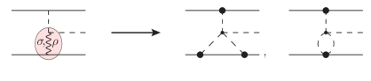
Figure 7: Diagram on the left-hand-side represents the phenomenological rescattering mechanism via the off shell $\pi N$-amplitude. Diagrams on the right-hand-side are the only loop graphs at N²LO that can be interpreted as an analog of this phenomenological mechanism. For notation see Fig. 1.

However, after the cancellations, the only contribution that survives from diagram IV has an isovector structure as shown in Table 1. Furthermore, the mini-football diagram gives an isovector contribution, see Table 2. Therefore, none of the pion loops can be mapped into the particular phenomenological mechanism in the isoscalar case. Thus, another lesson we learn from our work about the phenomenology of the neutral pion production near threshold is that the rescattering contribution with the isoscalar $\pi N$ amplitude modeled phenomenologically by a $\sigma$ exchange should be very small. On the other hand, the rescattering mechanism with the isovector $\pi N$ amplitude, the Weinberg–Tomozawa term related to the $\rho$-meson exchange via Kawarabayashi–Suzuki–Riazuddin–Fayyazuddin relation KS ; RF , is potentially capable of resolving the discrepancy with the experimental data for charged pion production lensky2 .

Appendix A The evaluation of the individual $g_{A}^{3}$-diagrams

In this appendix we derive the NLO and N²LO expressions for individual two-pion exchange diagrams shown in Fig. 3 under restriction that the outgoing pion is produced in s-wave. The kinematics is defined in Fig. 5.

A.1 Diagram II

Diagram II shown in Fig. 3 is straightforward to evaluate. The operator $A^{abc}_{g_{A}^{3}}$ of Eq. (9) in this case arises from a three-pion one-nucleon vertex whose explicit form can be found in Eqs. (5), (6). The diagram II yields the contribution

$$iM_{\text{II}} = \int\!\!\!\frac{d^{4}l}{(2\pi)^{4}}\,B_{2}(l,\tilde{l})\ \tau_{2}^{c}\tau_{2}^{b}\ \frac{g_{\!A}}{2f_{\!\pi}^{3}}\biggl{\{}[\tau_{1}^{a}\delta^{bc}S_{1}\cdot(-l+\tilde{l})+\tau_{1}^{b}\delta^{ac}S_{1}\cdot(q+\tilde{l})+\tau_{1}^{c}\delta^{ab}S_{1}\cdot(q-l)]$$

$$-\frac{1}{2m_{\!N}}i\varepsilon^{abc}[v\cdot qS_{1}\cdot(-l-\tilde{l})-v\cdot lS_{1}\cdot(\tilde{l}-q)+v\cdot\tilde{l}S_{1}\cdot(q+l)]$$

$$-\frac{1}{2m_{\!N}}S_{1}\cdot(p_{1}+p_{1}^{\,\prime})[\tau_{1}^{a}\delta^{bc}v\cdot(-l+\tilde{l})+\tau_{1}^{b}\delta^{ac}v\cdot(q+\tilde{l})+\tau_{1}^{c}\delta^{ab}v\cdot(q-l)]\biggr{\}},$$

where $B_{2}(l,\tilde{l})$ is defined in Eq. (10). Contracting isospin indexes and ignoring all p-wave terms ($\propto S_{1}\cdot q$) and higher-order s-wave terms $\propto v\cdot q/m_{\!N}\simeq m_{\pi}/m_{\!N}$ we find

$$iM_{\text{II}} = \frac{g_{\!A}}{4f_{\!\pi}^{3}}\int\!\!\!\frac{d^{4}l}{(2\pi)^{4}}\,B_{2}(l,\tilde{l})\biggl{\{}-(S_{1}\cdot l)[4\tau_{\!+}+4\tau_{\!-}-2\tau_{\!\times}]+(S_{1}\cdot\tilde{l})[4\tau_{\!+}+4\tau_{\!-}+2\tau_{\!\times}]$$

$$+\left[-\frac{S_{1}\cdot l}{2m_{\!N}}v\cdot\tilde{l}+\frac{S_{1}\cdot\tilde{l}}{2m_{\!N}}v\cdot l\right](2\tau_{\!+}-2\tau_{\!-})$$

$$+\frac{S_{1}\cdot(p_{1}+p_{1}^{\,\prime})}{2m_{\!N}}[v\cdot l(4\tau_{\!+}+4\tau_{\!-}-2\tau_{\!\times})-v\cdot\tilde{l}(4\tau_{\!+}+4\tau_{\!-}+2\tau_{\!\times})]\biggr{\}},$$

where the integrand in the first line starts to contribute at NLO while that in the last two lines gives N²LO contribution.

A.2 Diagram IIIa

The crossed box diagram, Type IIIa, shown in Fig. 3 has a more complicated structure. In this diagram the operator $A^{abc}_{g_{A}^{3}}$ consists of a $\pi N\to\pi N$ scattering vertex, a nucleon propagator and a $\pi NN$-vertex. Again we only need to include the contributions from the leading and subleading chiral Lagrangian in the vertices. We also include the nucleon recoil correction in the nucleon propagator. This diagram gives the following expression

$$iM_{\text{IIIa}} = \int\!\!\!\frac{d^{4}l}{(2\pi)^{4}}\,B_{2}(l,\tilde{l})\ \tau_{2}^{c}\tau_{2}^{b}\ \frac{1}{4f_{\!\pi}^{2}}\varepsilon^{bad}\tau_{1}^{d}\left(v\cdot(l+q)-\frac{(\vec{p}_{1}+\vec{p}_{1}^{\,\prime}-\vec{\tilde{l}})\cdot(\vec{l}+\vec{q})}{2m_{\!N}}\right)$$ (33)

$$\times\frac{i}{p_{10}-\tilde{l}_{0}-\frac{(\vec{p}_{1}-\vec{\tilde{l}})^{2}}{2m_{\!N}}+i0}\frac{g_{\!A}}{f_{\!\pi}}\tau_{1}^{c}\left(S_{1}\cdot\tilde{l}-\frac{S_{1}\cdot(2p_{1}-\tilde{l})v\cdot\tilde{l}}{2m_{\!N}}\right).$$

We have ignored here the subleading $c_{i}$-contributions to the $\pi N\to\pi N$ rescattering vertex since they are suppressed in the momentum counting scheme due to the negligible kinetic energy of the outgoing pion with $q\simeq(m_{\pi},\vec{0})$. We will rewrite the $\pi N\to\pi N$ vertex expression in the integrand above in a way similar to the rearrangement in Eq. (8)

$$v\cdot(l+q)-\frac{(\vec{p}_{1}+\vec{p}_{1}^{\,\prime}-\vec{\tilde{l}})\cdot(\vec{l}+\vec{q})}{2m_{\!N}}=$$

$$=-\left(p_{10}-\tilde{l}_{0}-\frac{(\vec{p}_{1}-\vec{\tilde{l}})^{2}}{2m_{\!N}}\right)+2q_{0}-\frac{2\vec{q}\cdot(\vec{p}_{1}+\vec{p}_{1}^{\,\prime}-\vec{\tilde{l}})}{2m_{\!N}},$$ (34)

where we used that $v\cdot p_{1}^{\prime}=p_{10}^{\,\prime}\simeq\vec{p}_{1}^{\,\prime}{}^{2}/2m_{\!N}$. The first term on the second line of Eq. (34) is identical to the nucleon propagator in Eq. (33) and will give a factor of $-1$ when inserted into Eq. (33). This factor of $-1$ together with the lowest-order contribution of the $\pi NN$-vertex, $S_{1}\cdot\tilde{l}$, give the NLO contribution of diagram IIIa. The last term in the second line of Eq. (34) contribute to an outgoing p-wave pion and is ignored in this paper. The $2q_{0}$ term in Eq. (34) will contribute to the N²LO amplitude. We next use the relation $\tilde{l}=l+p_{1}-p_{1}^{\,\prime}-q$ in the $\pi NN$-vertex and in the nucleon propagator. We ignore $p^{\prime}_{10}\sim q_{0}\sim m_{\pi}$ contributions and the recoil correction in the propagator which are of a higher order. Carrying out the isospin algebra we get:

$$iM_{\text{IIIa}} = \frac{g_{\!A}}{4f_{\!\pi}^{3}}\int\!\!\!\frac{d^{4}l}{(2\pi)^{4}}\,B_{2}(l,\tilde{l})\biggl{\{}(S_{1}\cdot\tilde{l})+\frac{S_{1}\cdot l}{2m_{\!N}}(v\cdot\tilde{l})$$

$$-\frac{S_{1}\cdot(p_{1}+p_{1}^{\,\prime})}{2m_{\!N}}(v\cdot\tilde{l})-\left(\frac{2v\cdot q}{-v\cdot l+i0}\right)\left(S_{1}\cdot\tilde{l}\right)\biggr{\}}[2\tau_{\!+}-\tau_{\!\times}]$$

The first term in the curly bracket starts to contribute at NLO. The remaining three terms contribute to N²LO.

A.3 Diagram IIIb

Diagram IIIb (Fig. 3) has a structure similar to diagram IIIa. We proceed along the same lines as for the two previous diagrams and obtain the following contribution:

$$iM_{\text{IIIb}} = \int\!\!\!\frac{d^{4}l}{(2\pi)^{4}}\,B_{2}(l,\tilde{l})\ \tau_{2}^{c}\tau_{2}^{b}(-1)\frac{g_{\!A}}{f_{\!\pi}}\tau_{1}^{b}\left(S_{1}\cdot l-\frac{S_{1}\cdot(2p_{1}^{\,\prime}-l)v\cdot l}{2m_{\!N}}\right)$$

$$\times\frac{i}{p_{10}^{\,\prime}-l_{0}-\frac{(\vec{p}_{1}^{\,\prime}-\vec{l})^{2}}{2m_{\!N}}+i0}\frac{1}{4f_{\!\pi}^{2}}\varepsilon^{cad}\tau_{1}^{d}\left(v\cdot(-\tilde{l}+q)-\frac{(\vec{p}_{1}+\vec{p}_{1}^{\,\prime}-\vec{l})\cdot(-\vec{\tilde{l}}+\vec{q})}{2m_{\!N}}\right)$$

Using the on-shell condition for the incoming nucleon with $p_{10}=\vec{p}_{1}{}^{\!\!2}/2m_{\!N}$, we rewrite the $\pi N\to\pi N$ vertex in a way similar to what was done for diagram IIIa

$$v\cdot(-\tilde{l}+q)-\frac{(\vec{p}_{1}+\vec{p}_{1}^{\,\prime}-\vec{l})\cdot(-\vec{\tilde{l}}+\vec{q})}{2m_{\!N}}=$$

$$=\left(p_{10}^{\,\prime}-l_{0}-\frac{(\vec{p}_{1}^{\,\prime}-\vec{l})^{2}}{2m_{\!N}}\right)+2q_{0}-\frac{2\vec{q}\cdot(\vec{p}_{1}+\vec{p}_{1}^{\,\prime}-\vec{l})}{2m_{\!N}}\,.$$ (35)

Using the relation $2q_{0}=2v\cdot q$ and keeping only terms appropriate at the order we are working we obtain:

$$iM_{\text{IIIb}} = \frac{g_{\!A}}{4f_{\!\pi}^{3}}\int\!\!\!\frac{d^{4}l}{(2\pi)^{4}}\,B_{2}(l,\tilde{l})\biggl{\{}(S_{1}\cdot l)+\frac{S_{1}\cdot\tilde{l}}{2m_{\!N}}(v\cdot l)$$

$$-\frac{S_{1}\cdot(p_{1}+p_{1}^{\,\prime})}{2m_{\!N}}(v\cdot l)+\left(\frac{2v\cdot q}{-v\cdot l+i0}\right)\left(S_{1}\cdot l\right)\biggr{\}}[-2\tau_{\!+}-\tau_{\!\times}]$$

The first term in the curly bracket starts to contribute at NLO. The remaining three terms contribute to N²LO.

A.4 Diagram IV

Diagram IV (Fig. 3) has an operator $A^{abc}_{g_{A}^{3}}$ containing a four-pion vertex, a pion propagator and one $\pi NN$-vertex. We keep the leading and next-to-leading order in the $\pi NN$-vertex and obtain

$$iM_{\text{IV}} = \int\!\!\!\frac{d^{4}l}{(2\pi)^{4}}\,B_{2}(l,\tilde{l})\ \tau_{2}^{c}\tau_{2}^{b}\left(\frac{g_{\!A}}{f_{\!\pi}}\right)\tau_{1}^{d}\left(S_{1}\cdot k_{1}-\frac{S_{1}\cdot(p_{1}+p_{1}^{\,\prime})v\cdot k_{1}}{2m_{\!N}}\right)\frac{i}{k_{1}^{2}-m_{\pi}^{2}+i0}$$

$$\times\frac{i}{f_{\!\pi}^{2}}\left\{\delta^{ab}\delta^{cd}\left[(l-q)^{2}-m_{\pi}^{2}\right]+\delta^{ac}\delta^{bd}\left[(\tilde{l}+q)^{2}-m_{\pi}^{2}\right]+\delta^{ad}\delta^{bc}\left[(k_{1}-q)^{2}-m_{\pi}^{2}\right]\right\}.$$

The four-pion vertex is rewritten as a sum of six terms

$$\frac{i}{f_{\!\pi}^{2}}\left\{\delta^{ab}\delta^{cd}\left[(l-q)^{2}-m_{\pi}^{2}\right]+\delta^{ac}\delta^{bd}\left[(\tilde{l}+q)^{2}-m_{\pi}^{2}\right]+\delta^{ad}\delta^{bc}\left[(k_{1}-q)^{2}-m_{\pi}^{2}\right]\right\}=$$

$$=\frac{i}{f_{\!\pi}^{2}}\biggl{\{}\delta^{ab}\delta^{cd}\left[l^{2}-m_{\pi}^{2}\right]+\delta^{ac}\delta^{bd}\left[\tilde{l}^{2}-m_{\pi}^{2}\right]+\delta^{ad}\delta^{bc}\left[k_{1}^{2}-m_{\pi}^{2}\right]+$$

$$+\delta^{ab}\delta^{cd}\left[-2l\cdot q+q^{2}\right]+\delta^{ac}\delta^{bd}\left[2\tilde{l}\cdot q+q^{2}\right]+\delta^{ad}\delta^{bc}\left[-2k_{1}\cdot q+q^{2}\right]\biggr{\}}.$$ (36)

The contributions from the first two terms on the r.h.s. of Eq. (36) are of a higher order. The reason is that each term cancels a corresponding pion propagator in the operator $B_{2}(l,\tilde{l})$. When one pion propagator in $B_{2}(l,\tilde{l})$ is eliminated, the large momentum, like $\vec{k}_{1}$ or $\vec{p}_{1}$, of this reaction is no longer part of the loop integral which, consequently, only contributes at a higher order than what is considered in this paper. Keep in mind that $v\cdot k_{1}$, $v\cdot p_{1}$ and $v\cdot p_{2}$ are all of the order $m_{\pi}$, whereas, $|\vec{k}_{1}|\sim p=\sqrt{m_{\pi}m_{\!N}}$. The third term cancels the pion propagator $k_{1}^{2}-m_{\pi}^{2}+i0$ and will contribute at NLO and higher order in our counting. The last three terms in Eq. (36) start contributing from N²LO.

Using $k_{1}=\tilde{l}-l+q$, dropping terms contributing to outgoing p-wave pions and carrying out the spin and isospin algebra we find:

$$iM_{\text{IV}} = \frac{g_{\!A}}{4f_{\!\pi}^{3}}\int\!\!\!\frac{d^{4}l}{(2\pi)^{4}}\,B_{2}(l,\tilde{l})\biggl{\{}\left[(S_{1}\cdot l)-(S_{1}\cdot\tilde{l})+\frac{S_{1}\cdot(p_{1}+p_{1}^{\,\prime})}{2m_{\!N}}\left(-v\cdot l+v\cdot\tilde{l}\right)\right]6(\tau_{\!+}+\tau_{\!-})$$

$$+\left(S_{1}\cdot k_{1}\right)\biggl{[}\frac{(l+\tilde{l})\cdot q}{k_{1}^{2}-m_{\pi}^{2}+i0}\biggr{]}(-8\tau_{\!\times})\biggr{\}}.$$

The first two terms in the first square bracket are NLO contributions. The remaining two terms are N²LO terms.

A.5 Box diagram a

In the expression for the Box a diagram (Fig. 3) we again rewrite the pion-nucleon rescattering vertex as a sum of two terms similar to what we did for the Type-III diagrams. One of the new terms will cancel nucleon propagator yielding an irreducible NLO contribution. In contrast to the derivation of the amplitude for the Type-III graphs, we here do not consider the contribution from the term with the (remaining) nucleon propagator since it is reducible and thus included in the initial $NN$ state interaction. Using again that the sum of the two lowest orders contribute to the vertices, we obtain from the box a diagram:

$$iM_{\text{Box a}} = \int\!\!\!\frac{d^{4}l}{(2\pi)^{4}}\,B_{2}(l,\tilde{l})\ \tau_{2}^{c}\tau_{2}^{b}\left(\frac{1}{4f_{\!\pi}^{2}}\right)\varepsilon^{cad}\tau_{1}^{d}\left(v\cdot(-\tilde{l}+q)-\frac{(\vec{p}_{1}+\vec{p}_{1}^{\,\prime}+\vec{l})\cdot(-\vec{\tilde{l}}+\vec{q})}{2m_{\!N}}\right)$$ (37)

$$\times\frac{i}{l_{0}+p_{10}-\frac{(\vec{p}_{1}+\vec{l})^{2}}{2m_{\!N}}}(-1)\frac{g_{\!A}}{f_{\!\pi}}\tau_{1}^{b}\left(S_{1}\cdot l-\frac{S_{1}\cdot(2p_{1}+l)v\cdot l}{2m_{\!N}}\right).$$

To rewrite the expression in the pion-nucleon rescattering vertex we again use that that $p_{1}^{\,\prime}$ is on-shell, i.e. $p_{10}^{\,\prime}=\vec{p}_{1}^{\,\prime}{}^{2}/2m_{\!N}$. The $\pi N\to\pi N$ vertex is rewritten as

$$v\cdot(-\tilde{l}+q)-\frac{(\vec{p}_{1}+\vec{p}_{1}^{\,\prime}+\vec{l})\cdot(-\vec{\tilde{l}}+\vec{q})}{2m_{\!N}}=$$

$$=-\left(l_{0}+p_{10}-\frac{(\vec{p}_{1}+\vec{l})^{2}}{2m_{\!N}}\right)+2q_{0}-\frac{2\vec{q}\cdot(\vec{p}_{1}+\vec{p}_{1}^{\,\prime}+\vec{l})}{2m_{\!N}}\,.$$

The first term on the r.h.s. of the above expression is identical to the nucleon propagator and will give a factor of $-1$ when inserted into Eq. (37). The last term is a p-wave pion contribution and is ignored. Also the $2q_{0}$-term does not need to be taken into account as it corresponds to a reducible contribution. Using $2p_{1}+l=\tilde{l}+(p_{1}+p_{1}^{\,\prime})+q$, ignoring the p-wave pion terms, and evaluating the spin and isospin structures, we find:

$$iM_{\text{Box a}}^{\text{irred.}}=\frac{g_{\!A}}{4f_{\!\pi}^{3}}\int\!\!\!\frac{d^{4}l}{(2\pi)^{4}}\,B_{2}(l,\tilde{l})\biggl{\{}-(S_{1}\cdot l)+\frac{S_{1}\cdot\tilde{l}}{2m_{\!N}}(v\cdot l)+\frac{S_{1}\cdot(p_{1}+p_{1}^{\,\prime})}{2m_{\!N}}(v\cdot l)\biggr{\}}[2\tau_{\!-}+\tau_{\!\times}]$$

A.6 Box diagram b

The Box b diagram given in Fig. 3 is very similar to the Box a diagram and the evaluation procedure is similar. We consider again only the irreducible contribution. The diagram gives:

$$iM_{\text{Box b}} = \int\!\!\!\frac{d^{4}l}{(2\pi)^{4}}\,B_{2}(l,\tilde{l})\ \tau_{2}^{c}\tau_{2}^{b}\left(\frac{g_{\!A}}{f_{\!\pi}}\right)\tau_{1}^{c}\left(S_{1}\cdot\tilde{l}-\frac{S_{1}\cdot(2p_{1}^{\,\prime}+\tilde{l})v\cdot\tilde{l}}{2m_{\!N}}\right)$$ (38)

$$\times\frac{i}{p_{10}^{\,\prime}+\tilde{l}_{0}-\frac{(\vec{p}_{1}^{\,\prime}+\vec{\tilde{l}})^{2}}{2m_{\!N}}}\frac{1}{4f_{\!\pi}^{2}}\varepsilon^{bad}\tau_{1}^{d}\left(v\cdot(l+q)-\frac{(\vec{p}_{1}+\vec{p}_{1}^{\,\prime}+\vec{\tilde{l}})\cdot(\vec{l}+\vec{q})}{2m_{\!N}}\right).$$

Again, rewriting the pion-nucleon rescattering vertex using that $p_{1}$ is on shell, $p_{10}=\vec{p}_{1}{}^{\!\!2}/2m_{\!N}$ leads to :

$$v\cdot(l+q)-\frac{(\vec{p}_{1}+\vec{p}_{1}^{\,\prime}+\vec{\tilde{l}})\cdot(\vec{l}+\vec{q})}{2m_{\!N}}=$$

$$=\left(p_{10}^{\,\prime}+\tilde{l}_{0}-\frac{(\vec{p}_{1}^{\,\prime}+\vec{\tilde{l}})^{2}}{2m_{\!N}}\right)+2q_{0}-\frac{2\vec{q}\cdot(\vec{p}_{1}+\vec{p}_{1}^{\,\prime}+\vec{\tilde{l}})}{2m_{\!N}}\,.$$ (39)

The first factor on the r.h.s. of the Eq. (39), when coupled with the nucleon propagator in Eq. (38), yields a factor of $1$ while the $2q_{0}$-term in Eq. (39) produces a reducible contribution included in the final $NN$ state interaction. Using the relation $2p_{1}^{\,\prime}+\tilde{l}=l+(p_{1}+p_{1}^{\,\prime})-q$, ignoring terms leading to outgoing p-wave pions and carrying out the spin and isospin algebra leads to:

$$iM_{\text{Box b}}^{\text{irred.}}=\frac{g_{\!A}}{4f_{\!\pi}^{3}}\int\!\!\!\frac{d^{4}l}{(2\pi)^{4}}\,B_{2}(l,\tilde{l})\biggl{\{}(S_{1}\cdot\tilde{l})-\frac{S_{1}\cdot l}{2m_{\!N}}(v\cdot\tilde{l})-\frac{S_{1}\cdot(p_{1}+p_{1}^{\,\prime})}{2m_{\!N}}(v\cdot\tilde{l})\biggr{\}}[2\tau_{\!-}-\tau_{\!\times}].$$

Like the final expression for the Box a diagram, the first term starts at NLO and the next two terms are the N²LO contributions to the amplitude.

Appendix B The evaluation of the individual $g_{A}$-diagrams

In this appendix we derive the expression for two-pion exchange diagram linear in $g_{A}$ for s-wave pions produced. The final expressions for the diagrams contain N²LO contributions. The kinematics is defined in Fig.  6.

B.1 The Football diagram

The two pion propagators are tied together in pion-nucleon scattering vertices at both nucleons. Since this loop diagram involve just pion propagators, we have an extra symmetry factor $1/2$ associated with the boson loop. The football diagram shown in Fig. 3 gives the following expression:

$$iM_{\text{F}} = \frac{1}{2}\int\!\!\!\frac{d^{4}l}{(2\pi)^{4}}\,D_{2}(l,\tilde{l})\ \varepsilon^{cby}\tau_{2}^{y}\left(\frac{g_{\!A}}{2f_{\!\pi}^{3}}\right)$$

$$\times\biggl{\{}[\tau_{1}^{a}\delta^{bc}S_{1}\cdot(-l+\tilde{l})+\tau_{1}^{b}\delta^{ac}S_{1}\cdot(q+\tilde{l})+\tau_{1}^{c}\delta^{ab}S_{1}\cdot(q-l)]$$

$$-\frac{1}{2m_{\!N}}i\varepsilon^{abc}[v\cdot qS_{1}\cdot(-l-\tilde{l})-v\cdot lS_{1}\cdot(\tilde{l}-q)+v\cdot\tilde{l}S_{1}\cdot(q+l)]$$

$$-\frac{1}{2m_{\!N}}S_{1}\cdot(p_{1}+p_{1}^{\,\prime})[\tau_{1}^{a}\delta^{bc}v\cdot(-l+\tilde{l})+\tau_{1}^{b}\delta^{ac}v\cdot(q+\tilde{l})+\tau_{1}^{c}\delta^{ab}v\cdot(q-l)]\biggr{\}}.$$

After performing some spin and isospin algebra, dropping terms corresponding to the outgoing p-wave pion and/or higher-order corrections we obtain

$$iM_{\text{F}} = i\frac{g_{\!A}}{8f_{\!\pi}^{3}}\int\!\!\!\frac{d^{4}l}{(2\pi)^{4}}\,D_{2}(l,\tilde{l})\biggl{\{}\left[(S_{1}\cdot l)+(S_{1}\cdot\tilde{l})\right](-2\tau_{\!\times})$$

$$+\left[\frac{S_{1}\cdot l}{2m_{\!N}}(v\cdot\tilde{l})-\frac{S_{1}\cdot\tilde{l}}{2m_{\!N}}(v\cdot l)\right](2\tau_{\!+}-2\tau_{\!-})+\frac{S_{1}\cdot(p_{1}+p_{1}^{\,\prime})}{2m_{\!N}}\left[v\cdot l+v\cdot\tilde{l}\right](2\tau_{\!\times})\biggr{\}}.$$

The obtained result requires some clarification. Looking naively at the first line in Eq. (B.1) one may conjecture that this diagram starts to contribute already at NLO. Indeed, assuming $l_{0}\sim|\vec{l}|\sim p$, the dimensional analysis gives

$$\frac{p}{f_{\!\pi}^{3}}\cdot\frac{1}{f_{\!\pi}^{2}p^{3}}\cdot\frac{p^{4}}{(4\pi)^{2}}\sim\frac{1}{f_{\!\pi}^{3}}\frac{p^{2}}{m_{\!N}^{2}}$$

where the three terms on the l.h.s. stand for the $3\pi NN$-vertex, the estimate of $D(l,\tilde{l})$ as follows from Eq. (17) and the integral measure, in order. Above we also used that $(4\pi f_{\!\pi})^{2}\simeq m_{\!N}^{2}$. On the other hand, a more careful analysis shows that the first line of the integral in Eq. (B.1), which appears at NLO, is

$$iM_{\text{F}}=\tau_{\!\times}\ \frac{g_{\!A}}{16f_{\!\pi}^{5}}\int\!\!\!\frac{d^{4}l}{(2\pi)^{4}}\,\frac{2l_{0}}{(l_{0}^{2}-\vec{l}^{2}+i0)(l_{0}^{2}-\vec{\tilde{l}}^{2}+i0)}\left[(S_{1}\cdot l)+(S_{1}\cdot\tilde{l})\right],$$

where we have used that $l_{0}\sim|\vec{l}|\sim p\gg m_{\pi}$ to drop all subleading contributions including the $1/m_{\!N}$ terms in the curly bracket of the integrand. This last integral, however, vanishes when integrating over $l_{0}$ because the numerator of the integrand is an odd function of $l_{0}$ whereas the denominator is an even one. The next-higher order contributions in Eq. (B.1) do not vanish. They scale as $m_{\pi}/p$ and $p/m_{\!N}$ compared to NLO and thus emerge at N²LO. Following the same lines, one can show that also the other diagrams of $g_{A}$-topology start to contribute at N²LO.

B.2 Diagram Ia

The double-scattering diagram Ia shown in Fig. 3 gives the following expression

$$iM_{\text{Ia}} = \int\!\!\!\frac{d^{4}l}{(2\pi)^{4}}\,D_{2}(l,\tilde{l})\varepsilon^{cby}\tau_{2}^{y}\left(\frac{1}{4f_{\!\pi}^{2}}\right)\varepsilon^{bad}\tau_{1}^{d}\left(v\cdot(l+q)-\frac{(\vec{p}_{1}+\vec{p}_{1}^{\,\prime}-\vec{\tilde{l}})\cdot(\vec{l}+\vec{q})}{2m_{\!N}}\right)$$

$$\times\frac{i}{p_{10}-\tilde{l}_{0}-\frac{(\vec{p}_{1}-\vec{\tilde{l}})^{2}}{2m_{\!N}}+i0}\left(\frac{g_{\!A}}{f_{\!\pi}}\right)\tau_{1}^{c}\left(S_{1}\cdot\tilde{l}-\frac{S_{1}\cdot(2p_{1}-\tilde{l})v\cdot\tilde{l}}{2m_{\!N}}\right).$$

In the $\pi N\to\pi N$ rescattering vertex (off nucleon 1) we included the leading WT vertex contribution together with its recoil correction. However, we dropped the subleading $c_{i}$-terms in this vertex since they are of higher order (see the discussion in the end of Sec. II.2). The $\pi N\to\pi N$ vertex expression is rewritten the same way as for diagram IIIa, shown in Eq. (34).

Using that $p_{10}^{\,\prime}=\vec{p}_{1}^{\,\prime}{}^{2}/2m_{\!N}$, collecting the spin structures and performing the isospin algebra we get:

$$iM_{\text{Ia}} = i\frac{g_{\!A}}{8f_{\!\pi}^{3}}\int\!\!\!\frac{d^{4}l}{(2\pi)^{4}}\,D_{2}(l,\tilde{l})\biggl{\{}-(S_{1}\cdot l)-(S_{1}\cdot\tilde{l})-\frac{S_{1}\cdot l}{2m_{\!N}}\left(v\cdot\tilde{l}\right)+\frac{S_{1}\cdot\tilde{l}}{2m_{\!N}}(v\cdot l)$$

$$+\frac{S_{1}\cdot(p_{1}+p_{1}^{\,\prime})}{2m_{\!N}}\left[v\cdot l+v\cdot\tilde{l}\right]+\frac{4v\cdot q}{-v\cdot l+i0}\left(S_{1}\cdot\tilde{l}\right)\biggr{\}}(\tau_{\!+}-\tau_{\!-}-\tau_{\!\times}).$$

This amplitude starts to contribute at N²LO, see discussion in Appendix B.1 for more details.

B.3 Diagram Ib

The double-scattering diagram Ib in Fig. 3 gives an initial expression:

$$iM_{\text{Ib}} = \int\!\!\!\frac{d^{4}l}{(2\pi)^{4}}\,D_{2}(l,\tilde{l})\varepsilon^{cby}\tau_{2}^{y}(-1)\frac{g_{\!A}}{f_{\!\pi}}\tau_{1}^{b}\left(S_{1}\cdot l-\frac{S_{1}\cdot(2p_{1}^{\,\prime}-l)v\cdot l}{2m_{\!N}}\right)$$

$$\times\frac{i}{p_{10}^{\,\prime}-l_{0}-\frac{(\vec{p}_{1}^{\,\prime}-\vec{l})^{2}}{2m_{\!N}}+i0}\frac{1}{4f_{\!\pi}^{2}}\varepsilon^{cad}\tau_{1}^{d}\left(v\cdot(-\tilde{l}+q)-\frac{(\vec{p}_{1}+\vec{p}_{1}^{\,\prime}-\vec{l})\cdot(-\vec{\tilde{l}}+\vec{q})}{2m_{\!N}}\right).$$

Again, the $\pi N\to\pi N$ vertex is rewritten as sum of two terms as for diagram IIIb, see Eq. (35). We follow the simplifications discussed for diagram IIIb, and use that $p_{10}=\frac{\vec{p}_{1}{}^{\!\!2}}{2m_{\!N}}$. Using again $l\to-\tilde{l}$ etc. to simplify the integrals containing the function $D_{2}(l,\tilde{l})$, collecting spin structures and performing the isospin algebra we get:

$$iM_{\text{Ib}} = i\frac{g_{\!A}}{8f_{\!\pi}^{3}}\int\!\!\!\frac{d^{4}l}{(2\pi)^{4}}\,D_{2}(l,\tilde{l})\biggl{\{}(S_{1}\cdot l)+(S_{1}\cdot\tilde{l})-\frac{S_{1}\cdot l}{2m_{\!N}}\left(v\cdot\tilde{l}\right)+\frac{S_{1}\cdot\tilde{l}}{2m_{\!N}}(v\cdot l)$$

$$-\frac{S_{1}\cdot(p_{1}+p_{1}^{\,\prime})}{2m_{\!N}}\left[v\cdot l+v\cdot\tilde{l}\right]+\frac{4v\cdot q}{-v\cdot l+i0}\left(S_{1}\cdot l\right)\biggr{\}}[\tau_{\!+}-\tau_{\!-}+\tau_{\!\times}].$$

This amplitude also starts to contribute at N²LO, see comment in Appendix B.1 for more details.

B.4 The Mini-Football diagram

The contribution of the mini-football diagram in Fig. 3 can be written as

$$iM_{\text{mF}} = \frac{1}{2}\int\!\!\!\frac{d^{4}l}{(2\pi)^{4}}\,D_{2}(l,\tilde{l})\ \varepsilon^{cby}\tau_{2}^{y}\left(\frac{g_{\!A}}{f_{\!\pi}}\right)\tau_{1}^{d}\left(S_{1}\cdot k_{1}-\frac{S_{1}\cdot(p_{1}+p_{1}^{\,\prime})v\cdot k_{1}}{2m_{\!N}}\right)\frac{i}{k_{1}^{2}-m_{\pi}^{2}+i0}$$

$$\times\frac{i}{f_{\!\pi}^{2}}\left\{\delta^{ab}\delta^{cd}\left[(l-q)^{2}-m_{\pi}^{2}\right]+\delta^{ac}\delta^{bd}\left[(\tilde{l}+q)^{2}-m_{\pi}^{2}\right]+\delta^{ad}\delta^{bc}\left[(k_{1}-q)^{2}-m_{\pi}^{2}\right]\right\}.$$

The four-pion vertex can be rewritten as a sum of six terms

$$\frac{i}{f_{\!\pi}^{2}}\left\{\delta^{ab}\delta^{cd}\left[(l-q)^{2}-m_{\pi}^{2}\right]+\delta^{ac}\delta^{bd}\left[(\tilde{l}+q)^{2}-m_{\pi}^{2}\right]+\delta^{ad}\delta^{bc}\left[(k_{1}-q)^{2}-m_{\pi}^{2}\right]\right\}=$$

$$=\frac{i}{f_{\!\pi}^{2}}\biggl{\{}\delta^{ab}\delta^{cd}\left[l^{2}-m_{\pi}^{2}\right]+\delta^{ac}\delta^{bd}\left[\tilde{l}^{2}-m_{\pi}^{2}\right]+\delta^{ad}\delta^{bc}\left[k_{1}^{2}-m_{\pi}^{2}\right]$$

$$+\delta^{ab}\delta^{cd}\left[-2l\cdot q+q^{2}\right]+\delta^{ac}\delta^{bd}\left[2\tilde{l}\cdot q+q^{2}\right]+\delta^{ad}\delta^{bc}\left[-2k_{1}\cdot q+q^{2}\right]\biggr{\}}.$$

Following the arguments outlined in the derivation of the contribution from diagram IV, see the discussion below Eq. (36), most terms either contribute to outgoing p-wave pions or higher orders in the chiral expansion. The final result reads:

$$iM_{\text{mF}}=i\frac{g_{\!A}}{8f_{\!\pi}^{3}}\int\!\!\!\frac{d^{4}l}{(2\pi)^{4}}\,D_{2}(l,\tilde{l})\left(S_{1}\cdot k_{1}\right)\biggl{\{}\frac{q\cdot(l+\tilde{l})}{k_{1}^{2}-m_{\pi}^{2}+i0}\biggr{\}}(8\tau_{\!\times}).$$

This amplitude starts to contribute at N²LO.

Appendix C Expressions for loop-integrals

In this appendix we provide expressions for loop integrals required to calculate the transition amplitude at N²LO. Using dimensional regularization and integration procedure described in Appendix E of Ref. ParkMinRho93 , we obtained the following results:

$$\frac{1}{i}\!\int\!\!\!\frac{d^{4}l}{(2\pi)^{4}}\frac{v\cdot(l+\tilde{l})S_{1}\cdot(l+\tilde{l})}{(l^{2}-m_{\pi}^{2}+i0)(\tilde{l}^{2}-m_{\pi}^{2}+i0)(-v\cdot l+i0)}\simeq 0,$$ (41)

$$\frac{1}{i}\!\int\!\!\!\frac{d^{4}l}{(2\pi)^{4}}\frac{v\cdot(l+\tilde{l})}{(l^{2}-m_{\pi}^{2}+i0)(\tilde{l}^{2}-m_{\pi}^{2}+i0)(-v\cdot l+i0)}\simeq-2J(k_{1}^{2}),$$ (42)

$$\frac{1}{i}\!\int\!\!\!\frac{d^{4}l}{(2\pi)^{4}}\frac{v\cdot(l+\tilde{l})\,q\cdot(l+\tilde{l})}{(l^{2}-m_{\pi}^{2}+i0)(\tilde{l}^{2}-m_{\pi}^{2}+i0)}\simeq 2k_{1}^{2}(v\cdot q)\left[-\frac{1}{6}J(k_{1}^{2})-\frac{1}{9}\frac{1}{(4\pi)^{2}}\right],$$ (43)

$$\frac{1}{i}\!\int\!\!\!\frac{d^{4}l}{(2\pi)^{4}}\frac{(S_{2}\cdot\tilde{l})\,(S_{2}\cdot l)\,S_{1}\cdot(l+\tilde{l})}{(l^{2}-m_{\pi}^{2}+i0)(\tilde{l}^{2}-m_{\pi}^{2}+i0)(-v\cdot l+i0)^{2}}\simeq-i\varepsilon^{\mu\nu\alpha\beta}k_{1\mu}S_{1\nu}v_{\alpha}S_{2\beta}J(k_{1}^{2}),$$ (44)

$$\frac{1}{i}\!\int\!\!\!\frac{d^{4}l}{(2\pi)^{4}}\frac{(S_{2}\cdot\tilde{l})\,(S_{2}\cdot l)}{(l^{2}-m_{\pi}^{2}+i0)(\tilde{l}^{2}-m_{\pi}^{2}+i0)(-v\cdot l+i0)^{2}}\simeq\frac{3}{4}J(k_{1}^{2})-\frac{1}{(4\pi)^{2}},$$ (45)

$$\frac{1}{i}\!\int\!\!\!\frac{d^{4}l}{(2\pi)^{4}}\frac{(S_{2}\cdot\tilde{l})\,(S_{2}\cdot l)\,q\cdot(l+\tilde{l})}{(l^{2}-m_{\pi}^{2}+i0)(\tilde{l}^{2}-m_{\pi}^{2}+i0)(-v\cdot l+i0)}\simeq v\cdot q\frac{k_{1}^{2}}{2}\left[-\frac{5}{12}J(k_{1}^{2})+\frac{1}{18}\frac{1}{(4\pi)^{2}}\right],$$ (46)

where integral $J(k_{1}^{2})$ is given by Eq. (15), and only the leading loop contributions for the s-wave pion in MCS are kept.

References

• (1) H. O. Meyer et al., Nucl. Phys. A 539 (1992) 633.
• (2) C. Hanhart, Phys. Rept.  397 (2004) 155.
• (3) D. Tsirkov et al. [COSY-ANKE Collaboration], arXiv:1112.3799 [nucl-ex].
• (4) S. Dymov et al. [COSY-ANKE Collaboration], arXiv:1112.3808 [nucl-ex].
• (5) D. S. Koltun and A. Reitan, Phys. Rev.  141 (1966) 1413.
• (6) T. S. H. Lee and D. O. Riska, Phys. Rev. Lett.  70 (1993) 2237.
• (7) C. J. Horowitz, H. O. Meyer and D. K. Griegel, Phys. Rev. C 49 (1994) 1337.
• (8) C. J. Horowitz, Phys. Rev. C 48 (1993) 2920.
• (9) J. A. Niskanen, Phys. Rev. C 53 (1996) 526.
• (10) V. Baru, C. Hanhart, M. Hoferichter, B. Kubis, A. Nogga and D. R. Phillips, Nucl. Phys. A 872 (2011) 69; Phys. Lett. B 694 (2011) 473.
• (11) E. Hernandez and E. Oset, Phys. Lett. B 350 (1995) 158.
• (12) C. Hanhart, J. Haidenbauer, A. Reuber, C. Schutz and J. Speth, Phys. Lett. B 358 (1995) 21.
• (13) C. Hanhart, J. Haidenbauer, M. Hoffmann, U.-G. Meißner and J. Speth, Phys. Lett. B 424 (1998) 8.
• (14) T. D. Cohen, J. L. Friar, G. A. Miller and U. van Kolck, Phys. Rev. C 53 (1996) 2661.
• (15) B. Y. Park, F. Myhrer, J. R. Morones, T. Meissner and K. Kubodera, Phys. Rev. C 53 (1996) 1519.
• (16) T. Sato, T. S. H. Lee, F. Myhrer and K. Kubodera, Phys. Rev. C 56 (1997) 1246.
• (17) C. da Rocha, G. Miller and U. van Kolck, Phys. Rev. C 61 (2000) 034613.
• (18) V. Dmitrasinovic, K. Kubodera, F. Myhrer and T. Sato, Phys. Lett. B 465 (1999) 43.
• (19) S. Ando, T. -S. Park and D. -P. Min, Phys. Lett. B 509 (2001) 253.
• (20) C. Hanhart, U. van Kolck and G. A. Miller, Phys. Rev. Lett.  85 (2000) 2905.
• (21) C. Hanhart and N. Kaiser, Phys. Rev. C 66 (2002) 054005.
• (22) J. A. Niskanen, Nucl. Phys. A 298 (1978) 417.
• (23) C. Hanhart, J. Haidenbauer, O. Krehl and J. Speth, Phys. Lett. B 444 (1998) 25.
• (24) C. Hanhart, J. Haidenbauer, O. Krehl and J. Speth, Phys. Rev. C 61 (2000) 064008.
• (25) V. Baru, J. Haidenbauer, C. Hanhart, A. E. Kudryavtsev, V. Lensky and U.-G. Meißner, eConfC 070910 (2007) 128.
• (26) V. Baru, E. Epelbaum, J. Haidenbauer, C. Hanhart, A. E. Kudryavtsev, V. Lensky and U.-G. Meißner, Phys. Rev. C 80 (2009) 044003.
• (27) V. Lensky, V. Baru, J. Haidenbauer, C. Hanhart, A. E. Kudryavtsev and U.-G. Meißner, Eur. Phys. J. A 27 (2006) 37.
• (28) C. Hanhart and A. Wirzba, Phys. Lett. B 650 (2007) 354.
• (29) Y. Kim, T. Sato, F. Myhrer and K. Kubodera, Phys. Rev. C 80 (2009) 015206.
• (30) V. Bernard, N. Kaiser and U.-G. Meißner, Eur. Phys. J. A 4 (1999) 259.
• (31) C. Ordóñez, L. Ray and U. van Kolck, Phys. Rev. C 53 (1996) 2086.
• (32) V. Bernard, N. Kaiser and U.-G. Meißner, Int. J. Mod. Phys. E 4 (1995) 193.
• (33) N. Fettes, U.-G. Meißner, M. Mojzis and S. Steininger, Annals Phys.  283 (2000) 273 [Erratum-ibid.  288 (2001) 249].
• (34) D. R. Bolton and G. A. Miller, Phys. Rev. C 83 (2011) 064003.
• (35) R. A. Arndt, W. J. Briscoe, I. I. Strakovsky and R. L. Workman, Phys. Rev. C 76 (2007) 025209.
• (36) A. Gårdestig, D. R. Phillips and C. Elster, Phys. Rev. C 73 (2006) 024002.
• (37) U. van Kolck, G. A. Miller and D. O. Riska, Phys. Lett. B 388 (1996) 679.
• (38) A. Filin et al., in preparation
• (39) R. Shyam and U. Mosel, Phys. Lett. B 426 (1998) 1.
• (40) K. Kawarabayashi and M. Suzuki, Phys. Rev. Lett.  16 (1966) 255.
• (41) Riazuddin and Fayyazuddin, Phys. Rev.  147 (1966) 1071.
• (42) T.-S. Park, D.-P. Min and M. Rho, Phys. Rept.  233 (1993) 341.