Lagrangian chaos in an ABC–forced nonlinear dynamo

Abstract

The Lagrangian properties of the velocity field in a magnetized fluid are studied using three-dimensional simulations of a helical magnetohydrodynamic dynamo. We compute the attracting and repelling Lagrangian coherent structures, which are dynamic lines and surfaces in the velocity field that delineate particle transport in flows with chaotic streamlines and act as transport barriers. Two dynamo regimes are explored, one with a robust coherent mean magnetic field and one with intermittent bursts of magnetic energy. The Lagrangian coherent structures and the statistics of finite–time Lyapunov exponents indicate that the stirring/mixing properties of the velocity field decay as a linear function of the magnetic energy. The relevance of this study for the solar dynamo problem is discussed.

Keywords: Lagrangian coherent structures, MHD, dynamo

1 Introduction

Transport in chaotic flows is governed by a combination of stirring and diffusion. Stirring refers to the transport, stretching, twisting and folding of fluid elements and, consequently, of scalar or vector quantities advected by the flow, such as temperature, light particles or magnetic field lines in a magnetohydrodynamic (MHD) system. This process creates complex tracer patterns in the flow, including filaments and sheets, as the fluid elements are deformed in different directions. Diffusion is responsible for homogenizing the distribution of tracers and blurring the patterns created by the chaotic stirring, being usually more important in small scales [1]. This paper deals with the problem of chaotic stirring in magnetized flows. Throughout the paper we use the terms “stirring” and “mixing” interchangeably.

Passive scalars are quantities that are passively advected by the flow, i.e., their back–reaction on the advecting velocity field is disregarded. They constitute a powerful way to study transport in hydrodynamical and MHD flows (for a review, see Falkovich et al. [2]). We employ passive scalars to investigate how the magnetic field can affect particle transport and the stirring/mixing properties of a velocity field in MHD simulations through the Lorentz force. We adopt direct numerical simulations of resistive three–dimensional (3–D) compressible MHD equations with a helical forcing, which has been used elsewhere as a prototype of the $\alpha^{2}$ dynamo model of mean field dynamo theory [3, 4].

In the Lagrangian approach to turbulent transport the dynamics of fluids is studied by following the trajectories of a large number of fluid elements or tracer particles. The specific trajectories of individual particles are not very useful in this type of investigation in chaotic flows, since sensitivity to initial conditions means that particles that are arbitrarily close may experience exponential divergence with time. However, it is possible to detect certain material lines in the flow that repel or attract fluid elements. These repelling and attracting material lines are time–dependent analogous to the stable and unstable manifolds of hyperbolic fixed points in dynamical systems theory and form transport barriers in flows with chaotic streamlines, being called Lagrangian coherent structures (LCS). The LCS have been used to describe hydrodynamic turbulence in 3–D numerical simulations [5], laboratory experiments [6, 7] and observational data of oceans [8, 9] and the atmosphere [10], as well as 2–D numerical simulations of magnetized fusion plasmas [11], magnetic reconnection [12], and 3–D MHD simulations of conservative [13] and dissipative [4] fields.

One of the most widely used Lagrangian tools are the finite-time Lyapunov exponents (FTLE), also known as direct Lyapunov exponents. The FTLE are a measure of local chaos and quantify the dispersion of particles in a region of the flow during a finite time. In the context of dynamo theory, the stretching rate of material lines in a fluid can be used to explain the amplification of magnetic fields by the mechanism of stretch–twist–fold dynamo [14]. Examples of applications of the FTLE in dynamo simulations include the growth of seed magnetic fields in the kinematic dynamo problem [15, 16, 17], nonlinear MHD dynamos [18, 19, 20] and the amplification of interstellar magnetic fields and turbulent mixing by supernova–driven turbulence in compressible MHD simulations [21]. It was shown by Haller [22] that FTLE can also be used to identify repelling and attracting Lagrangian coherent structures.

We present the detection of Lagrangian coherent structures for two different dynamo regimes in the 3–D compressible MHD equations with the isotropic and helical ABC forcing. We focus on the change in transport and mixing properties of the flow when the system undergoes a transition whereby a large–scale spatially coherent magnetic field loses its stability. The transition, which occurs after an increase in the magnetic diffusivity, results in strongly intermittent time series of magnetic energy. In the intermittent regime, the lower magnetic energy causes chaotic mixing to increase, resulting in higher stretching rates of material lines. Chaotic mixing is quantified by the finite–time Lyapunov exponents, which show a linear dependence on the magnetic energy. In section II of this paper we define Lagrangian coherent structures and how they relate to chaotic stirring in fluids; Section III describes the model of MHD dynamo adopted; the numerical analysis is discussed in section IV and section V presents the conclusions and possible ways to apply our techniques to observational data of the solar dynamo.

2 Lagrangian Coherent Structures

Let $D\subset\mathbb{R}^{3}$ be the domain of the fluid to be studied, let $\mathbf{x}(t_{0})\in D$ denote the position of a passive particle at time $t_{0}$ and let $\mathbf{u}(\mathbf{x},t)$ be the velocity field defined on $D$. The motion of the particle is given by the solution of the initial value problem

$$\mathbf{\dot{x}}=\mathbf{u}(\mathbf{x},t),\qquad\mathbf{x}(t_{0})=\mathbf{x}_{0}.$$ (1)

Let us define the following flow map: $\phi_{t_{0}}^{t_{0}+\tau}:\mathbf{x}(t_{0})\mapsto\mathbf{x}(t_{0}+\tau)$. The deformation gradient is given by $J=\mathrm{d}\phi_{t_{0}}^{t_{0}+\tau}(\mathbf{x})/\mathrm{d}\mathbf{x}$ and the finite-time right Cauchy-Green deformation tensor is given by $\triangle=J^{T}J$. Let $\lambda_{1}>\lambda_{2}>\lambda_{3}$ be the eigenvalues of $\triangle$. Then, the finite-time Lyapunov exponents or direct Lyapunov exponents of the trajectory of the particle are defined as [23]:

$$\sigma_{i}^{t_{0}+\tau}(\mathbf{x})=\frac{1}{|\tau|}\ln\sqrt{\lambda_{i}},\qquad i=1,2,3.$$ (2)

The maximum FTLE gives the finite-time average of the maximum rate of divergence or stretching between the trajectories of a fiducial particle at $\mathbf{x}$ and its neighboring particles. The maximum stretching is found when the neighboring particle $\mathbf{y}$ is such that $\delta\mathbf{x}=\mathbf{x}-\mathbf{y}$ is initially aligned with the eigenvector of $\triangle$ associated with $\lambda_{1}$. A positive $\sigma_{1}$ is the signature of chaotic streamlines in the velocity field. The other exponents provide information about stretching/contraction in other directions and can be useful to interpret the local dynamics of the fluid. In an ideal conductive fluid, the frozen-in condition implies that a magnetic line aligned with an infinitesimal vector connecting two close fluid elements will evolve as this vector [24]. As pointed out by Balsara et al. [21], for finite resistivity and compressible flows, flow regions with three positive Lyapunov exponents expand in all three directions and tend to dilute out the magnetic field; regions with two positive Lyapunov exponents and one negative exponent tend to concentrate the magnetic fields into sheet–like structures; regions with one positive and two negative exponents tend to mold the magnetic fields into filamentary structures; compression in all directions is found when all exponents are negative. On the other hand, local minima in the maximum FTLE field might provide a way to detect the position of the center of vortices in the velocity field, since vortices may be viewed as material tubes of low particle dispersion [25].

Finite-time Lyapunov exponents are also useful to detect attracting and repelling material lines that act as barriers to particle transport in the velocity field. A material line is a smooth curve of fluid particles advected by the velocity field [22]. These attracting and repelling material lines are the analogous of stable and unstable manifolds of time-independent fields. The study of 2–D flows is helpful to understand the role of material lines. Consider a 2–D steady flow, where the velocity field does not change with time. In the presence of counter–rotating vortices, hyperbolic (saddle) points are expected to be found, such as the one illustrated in Fig. 1(a). The trajectories of passive scalars follow the velocity vectors in the vicinity of the hyperbolic point. Thus, particles lying on the stable manifold (green line) are attracted to the saddle point in the forward–time dynamics and trajectories on the unstable manifold (red line) converge to the saddle point in the backward–time dynamics.

Two particles are said to straddle a manifold if the line segment connecting them crosses the manifold. The maximum FTLE has particularly high values on the stable manifold in forward–time, since nearby trajectories straddling the manifold will experience exponential divergence when they approach the saddle point, as shown in Fig. 1(b). Similarly, the FTLE field exhibits a local maximizing curve (ridge) along the unstable manifold in backward–time dynamics, since trajectories straddling the unstable manifold diverge exponentially when they approach the saddle point in reversed–time, as in Fig. 1(c). Thus, ridges in the forward–time FTLE field mark the stable manifolds of hyperbolic points and ridges in the backward–time FTLE field mark the unstable manifolds.

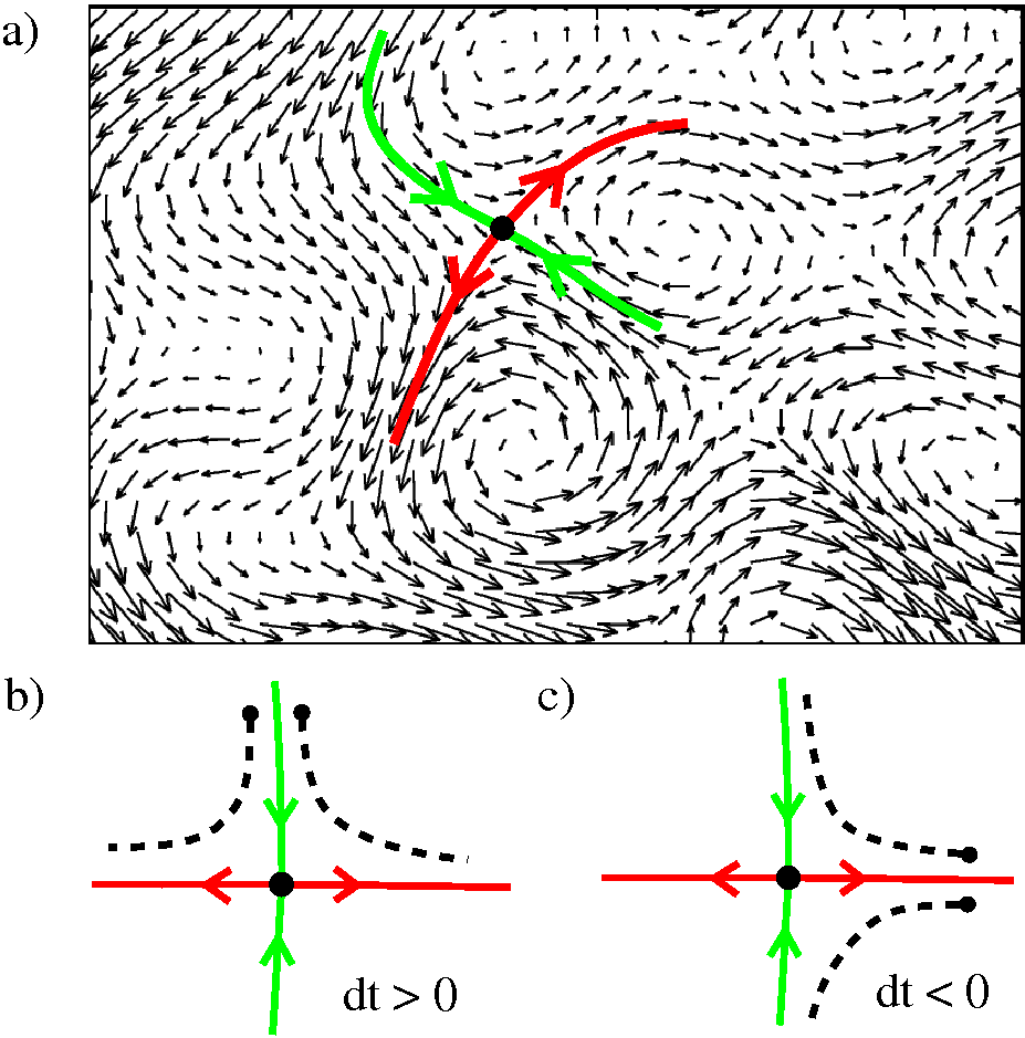
Figure 1: (Color online) (a) Velocity vector field with a saddle point (black circle) and its stable (green) and unstable (red) manifolds; (b) schematic drawing of the forward–time trajectories (dashed lines) of two passive particles that straddle the stable manifold of a saddle point; (c) schematic drawing of the backward–time trajectories (dashed lines) of two passive particles that straddle the unstable manifold of a saddle point.

Analogously, for a time-dependent velocity field, regions of maximum material stretching generate ridges in the FTLE field. Thus, repelling material lines (finite-time stable manifolds) produce ridges in the maximum FTLE field in the forward-time system and attracting material lines (finite-time unstable manifolds) produce ridges in the backward-time system [11, 22, 23]. These material lines are called Lagrangian coherent structures (LCS).

Stable and unstable manifolds are invariant sets, which means that a particle on the manifold will stay on it for all time. They form natural barriers to transport between different regions of a fluid, as seen in Figure 2. Figure 2(a) shows a topological configuration where one branch of the unstable manifold of the saddle point $S_{1}$ smoothly joins the stable manifold of another saddle point $S_{2}$ in a heteroclinic connection. Simultaneously, the two branches of the unstable manifold of $S_{2}$ are connected to the stable manifold of $S_{1}$, enclosing regions $A$ and $B$. Particles trapped in $A$ or $B$ cannot cross the barriers formed by the manifolds, since these are invariant sets. Figure 2(b) shows another type of trapping region, formed by a homoclinic connection, where one branch of the unstable manifold of a saddle point joins its own stable manifold. Trajectories in regions $A$ and $B$ usually circulate around a focus, as the manifolds mark the borders of vortices in the velocity field. Transport between different vortices is only possible when there is a transversal crossing between stable and unstable manifolds, through a mechanism called lobe dynamics [26, 27]. It is easier to understand this mechanism with a periodic flow. Suppose that the velocity field is time–dependent but periodic, such that $\mbox{\bf u}(\mbox{\bf x},t)=\mbox{\bf u}(\mbox{\bf x},t+T)$, where $T$ is the period. Let $F$ be the stroboscopic Poincaré map defined by $F(\mbox{\bf x}(t))=\phi_{t}^{t+T}(\mbox{\bf x})$. There are still points where the velocity is instantly zero, but now they are moving. Since these points are not fixed, they are called stagnation points. After $T$ time units a stagnation point will return to its original position. Therefore, under the map $F$ a stagnation point is seen as a fixed point. Figure 2(c) shows a heteroclinic tangle, where two hyperbolic fixed points of $F$ have associated stable and unstable manifolds which intersect in a number of points, forming a set of lobes that protrude from one region to the other. At time $t_{0}$, lobes $A_{1}$ and $A_{2}$ belong to region $A$ and lobes $B_{1}$ and $B_{2}$ to region $B$. Particles trapped in each lobe cannot cross their bordering manifolds, but as time goes by the dynamic manifolds are transported and deformed by the flow, since they are material lines. After one period, lobe $A_{1}$ is mapped onto the lobe marked as $F(A_{1})$, which belongs to region $B$. The same happens to lobe $A_{2}$, which is mapped onto $F(A_{2})$. Further iterations of the Poincaré map $F$ may cause lobes $F(A_{1})$ and $F(A_{2})$ to be deeply immersed into region $B$. Similarly, lobes $B_{1}$ and $B_{2}$ in region $B$ are mapped to lobes $F(B_{1})$ and $F(B_{2})$ in region $A$.

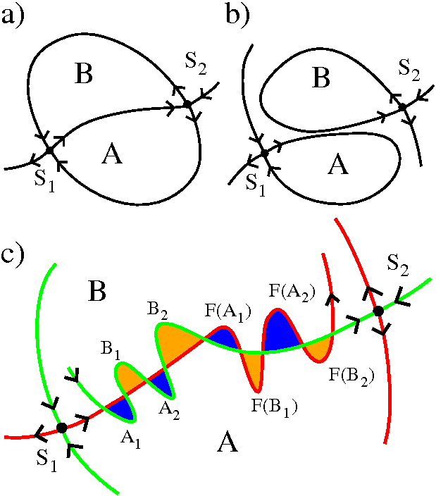
Figure 2: (Color online) (a) Heteroclinic connection between saddle points $S_{1}$ and $S_{2}$. There can be no transport of scalars between regions $A$ and $B$. (b) Homoclinic connections. Again, there is no transport between regions $A$ and $B$. (c) Heteroclinic tangle between the unstable manifold of $S_{1}$ and the stable manifold of $S_{2}$. The transport of particles between regions $A$ and $B$ is possible through lobe dynamics.

3 The model

A compressible isothermal gas is considered, with constant sound speed $c_{s}$, constant dynamical viscosity $\mu$, constant magnetic diffusivity $\eta$, and constant magnetic permeability $\mu_{0}$. The following set of compressible MHD equations is solved

$$\partial_{t}\ln\rho+\mathbf{u}\cdot\nabla\ln\rho+\nabla\cdot\mathbf{u}=0,$$ (3)

$$\partial_{t}\mathbf{u}+\mathbf{u\cdot}\nabla\mathbf{u}=-\nabla p/\rho+\mathbf{J\times B}/\rho+(\mu/\rho)\left(\nabla^{2}\mathbf{u}+\nabla\nabla\cdot\mathbf{u}/3\right)+\mathbf{f},$$ (4)

$$\partial_{t}\mathbf{A}=\mathbf{u\times B}-\eta\mu_{0}\mathbf{J},$$ (5)

where $\rho$ is the density, $\mathbf{u}$ is the fluid velocity, $\mathbf{A}$ is the magnetic vector potential, $\mathbf{J}=\nabla\times\mathbf{B}/\mu_{0}$ is the current density, $p$ is the pressure, $\mathbf{f}$ is an external forcing, and $\nabla p/\rho=c_{s}^{2}\nabla\ln\rho$, where $c_{s}^{2}=\gamma p/\rho$ is assumed to be constant. Nondimensional units are adopted, such that $c_{s}=\rho_{0}=\mu_{0}=1$, where $\rho_{0}=\left<\rho\right>$ is the spatial average of $\rho$. Equations (3)–(5) are solved with the PENCIL CODE in a box with sides $L=2\pi$ and periodic boundary conditions, so the smallest wavenumber is $k_{1}=1$. The time unit is $(c_{s}k_{1})^{-1}$ and the unit of viscosity $\nu$ and magnetic diffusivity $\eta$ is $c_{s}/k_{1}$. The initial conditions are $\ln\rho=\mathbf{u}=0$, and $A$ is a set of normally distributed, uncorrelated random numbers with zero mean and standard deviation equal to $10^{-3}$. The forcing function $\mathbf{f}$ is given by the strongly helical ABC flow,

$$\mathbf{f(x)}=\frac{A_{f}}{\sqrt{3}}[\sin k_{f}z+\cos k_{f}y,\sin k_{f}x+\cos k_{f}z,\sin k_{f}y+\cos k_{f}x],$$ (6)

where $A_{f}$ is the amplitude and $k_{f}$ the wavenumber of the forcing function.

Following Rempel et al. [3, 4], we use $A_{f}=0.1$, $k_{f}=5$, and the numerical resolution varies between $64^{3}$ and $128^{3}$. Spatial averages are denoted by $\left<\cdot\right>$ and time averages by $\left<\cdot\right>_{t}$. References to kinetic $(Re)$ and magnetic $(Rm)$ Reynolds numbers are based on the forcing scale

$$Re=\lambda_{f}U/\nu,\qquad Rm=\lambda_{f}U/\eta,$$ (7)

where $\nu=\mu/\rho_{0}$ is the average kinematic viscosity, $\lambda_{f}=2\pi/k_{f}$ is the forcing spatial scale, and $U=\left<u^{2}\right>^{1/2}$ is the mean velocity at a time when the magnetic field is saturated. The turnover time $\tau=\lambda_{f}/u_{rms}$ varies between $\tau\approx 3$ and $\tau\approx 4.5$ for our range of $\eta$.

4 Results

4.1 Bifurcation diagrams

We choose $\eta$ as the control parameter and fix $\nu=0.005$, which in the absence of magnetic fields corresponds to a spatiotemporally chaotic flow with $Re\approx 100$. Figure 3(a) shows the bifurcation diagrams for the time–averaged magnetic ($\left<E_{m}\right>_{t}$, red triangles) and kinetic ($\left<E_{k}\right>_{t}$, black circles) energies as a function of $\eta$ (lower axes) or $Rm$ (upper axes). Averages are computed after an initial transient is dropped. For large values of $\eta$, the seed magnetic field decays rapidly and there is no dynamo. At the onset of dynamo action at $\eta\sim 0.053$ ($Rm\sim 9.5$), the magnetic energy starts to grow at the expense of kinetic energy, until it saturates. Figure 3(b) shows in the upper panel the time–averaged kinetic helicity, $H_{k}=\left<\mathbf{u}\cdot\mathbf{\omega}\right>$, where $\mathbf{\omega}=\nabla\times\mathbf{u}$ is the vorticity, and in the lower panel the time–averaged magnetic helicity, $H_{m}=\left<\mathbf{A}\cdot\mathbf{B}\right>$. For helically forced flows, the magnetic helicity is expected to have the same sign as the kinetic helicity in scales smaller than the energy injection scale and the opposite sign in larger scales [28]. Most of the magnetic helicity in our simulations is concentrated in large scales, as happens with the magnetic energy [3], thus, $H_{m}$ has the opposite sign as $H_{k}$ in Fig. 3(b). These quantities are crucial for the emergence of a large–scale mean field, as they are related to the $\alpha$–effect in mean–field dynamo theory, which is responsible for the generation of a mean electromotive force along the mean magnetic field by turbulent fluctuations of the velocity and magnetic fields [29, 30]. The presence of kinetic helicity is thought to be responsible for the inverse transfer of magnetic energy from small scales to large scales, as well as the inverse transfer of magnetic helicity from the energy injection scale to larger scales [28]. In Fig. 3(b), $H_{k}$ is high for large values of $\eta$ and $H_{m}$ is null, since there is no dynamo and a maximally helical (Beltrami) forcing is applied to the flow. After the onset of dynamo, the magnetic field starts to contribute to the flow dynamics through the Lorentz force (second term at the right in Eq. 4) and $H_{k}$ decreases with $\eta$, as $\left|H_{m}\right|$ grows.

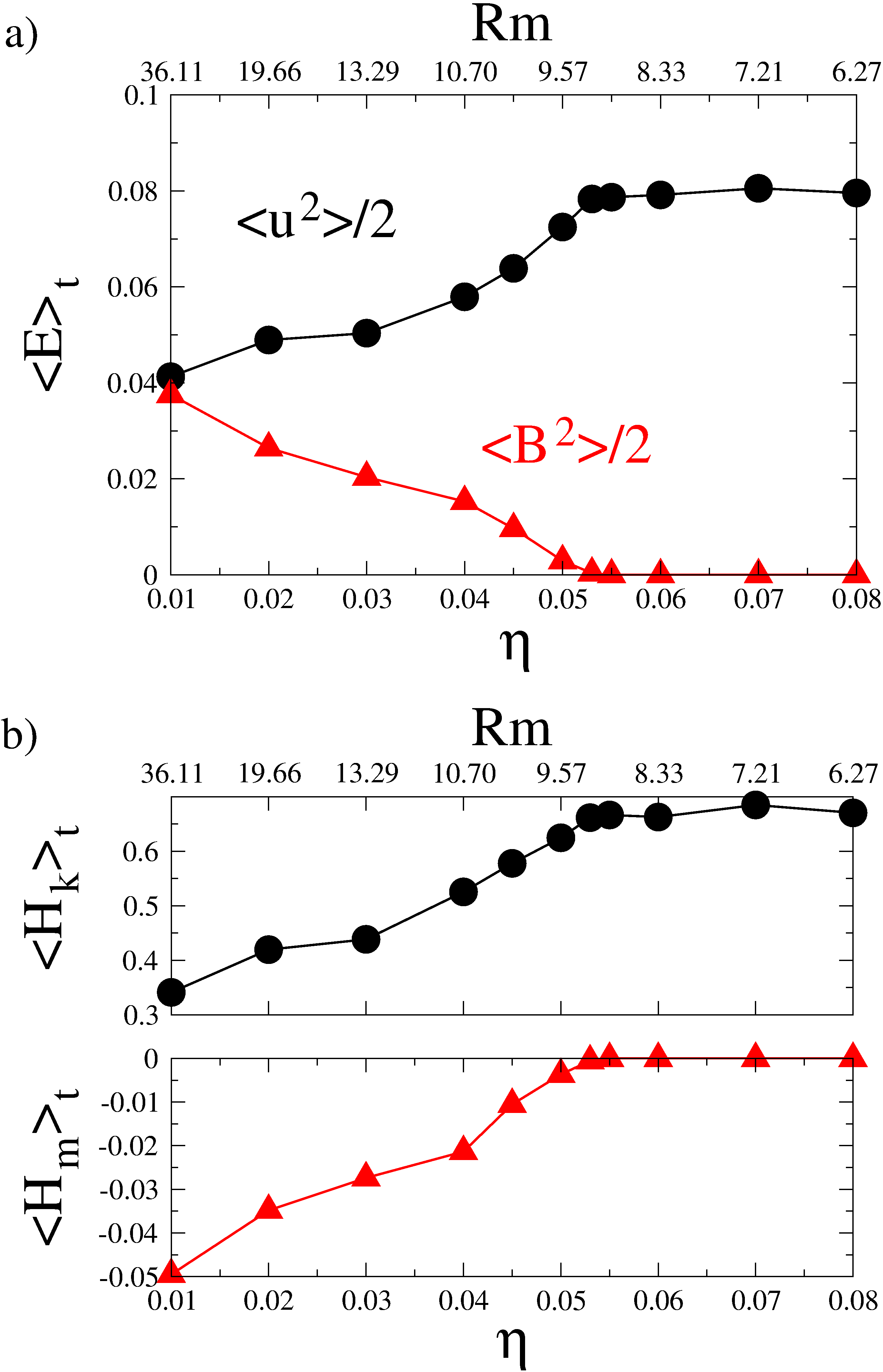
Figure 3: (Color online) Bifurcation diagrams as a function of $\eta$: (a) kinetic (black circles) and magnetic (red triangles) energies; (b) kinetic (black circles) and magnetic (red triangles) helicities.

We focus on two values of $\eta$. For $\eta=0.01$ the magnetic field is close to equipartition after saturation, as seen in the comparison between the time series of $B_{\rm rms}$ and $u_{\rm rms}$ in Fig. 4. For $\eta=0.05$, close to the onset of dynamo action, the magnetic energy is almost an order of magnitude smaller than the kinetic energy and the time series are strongly intermittent, as shown in Fig. 5. Two pairs of vertical lines in Fig. 5 mark the beginning and apex of two bursts of magnetic energy around times $t=2400$ and $t=6000$. This is a type of on–off intermittency due to a blow–out bifurcation, as discussed by Rempel et al. [3].

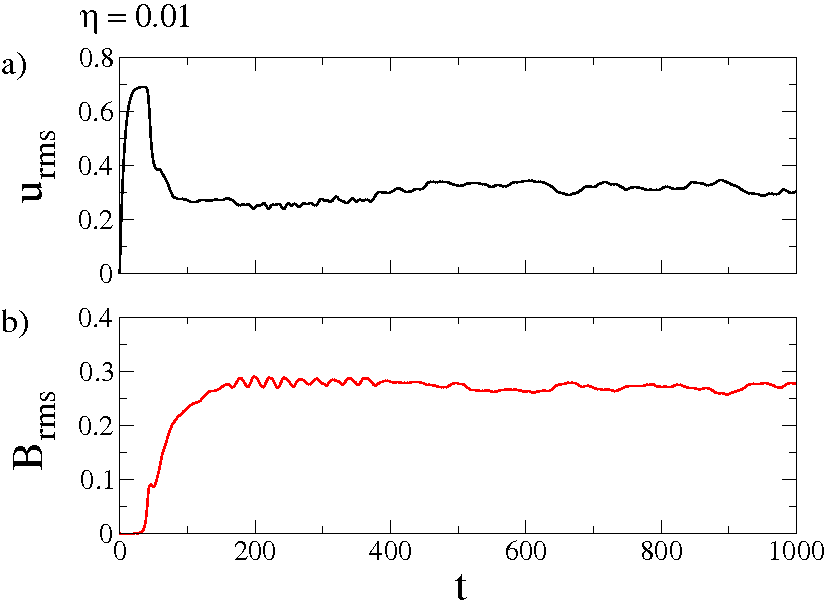
Figure 4: (Color online) Time series for $u_{\rm rms}$ (upper panel) and $B_{\rm rms}$ (lower panel) for $\nu=0.005$ and $\eta=0.01$.

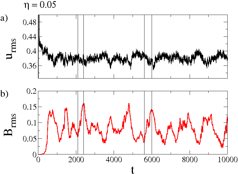
Figure 5: (Color online) Time series for $u_{\rm rms}$ (upper panel) and $B_{\rm rms}$ (lower panel) for $\nu=0.005$ and $\eta=0.05$.

The magnetic field structures are depicted in Fig. 6 for the two values of $\eta$ and different times. For $\eta=0.01$ (upper panel) there is a robust coherent large–scale $B_{z}$ component accompanied by small–scale turbulent fluctuations. For $\eta=0.05$ (lower panel), the magnetic field displays an intermittent switching between coherent and incoherent large-scale structures [Fig. 6(b)] and there is no preferred direction for field alignment.

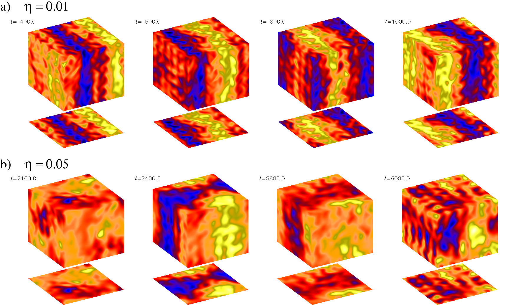
Figure 6: (Color online) (a) Intensity plots of $B_{z}$ at four different times, showing the evolution of a large-scale coherent pattern modulated along the $x$ direction for $\eta=0.01$; (b) same as (a) but for $\eta=0.05$, showing intermittent switching between ordered and disordered patterns.

4.2 Lagrangian analysis

The contrast between the Eulerian and Lagrangian analyses is depicted in Figure 7 for $\eta=0.01$, when the magnetic field has settled to a spatially regular mean field. Figure 7(a) shows the line integral convolution (LIC) plot [31] for the velocity field at $z=0$. The LIC plot reveals the streamlines of the $(u_{x},u_{y})$ velocity components on this plane at $t=1000$. Arrays of counter–rotating vortices found in the ABC–flow can still be seen, intermixed with long streaks and displaced vortices. To obtain the Lagrangian coherent structures we compute the maximum FTLE field. For the attracting LCS (finite–time unstable manifolds) we need to integrate the compressible MHD equations backward in time, which is a major problem, since the system is dissipative. We resort to interpolation of recorded data to compute these fields. A run of Eqs. (3)–(5) from $t_{0}-\tau$ to $t_{0}+\tau$ is conducted and full three-dimensional snapshots of the velocity fields are saved at each $dt=0.5$ time interval. Following [11] and [32], linear interpolation in time and third order Hermite interpolation in space is used to obtain the continuous set of vector fields necessary to obtain the particle trajectories by integration of Eq. (1). For backward integration, $\mathbf{\dot{x}}=-\mathbf{u}(\mathbf{x},t)$ is solved instead, as snapshots are read from $t_{0}$ to $t_{0}-\tau$. Figure 7(b) shows the backward–time maximum FTLE field computed with $\tau=-10$ and $t_{0}=1000$. Bright colors correspond to large values of $\sigma_{1}$ and dark regions to low values. The ridges seen as bright red lines approximate the attracting LCS. Figure 7(c) shows the forward–time maximum FTLE field for $\tau=10$, whose ridges provide the repelling LCS. Figure 7(d) is a superposition of (b) and (c), and represents the so–called “Lagrangian skeleton of turbulence” [32]. Figures 7(e) and 7(f) are enlargements of the square regions in Figs. 7(a) and 7(d), respectively. Note that the LIC plot of the velocity field in Fig. 7(e) shows a structure similar to the homoclinic connections of Fig. 2(b). Here, the arrows point to two hyperbolic stagnation points in the $(u_{x},u_{y})$ field. On the other hand, when one moves to the Lagrangian frame (Fig. 7(f)) the picture becomes much more complex, with a number of homoclinic and heteroclinic crossings, as in Fig. 2(c). The two larger arrows point to the same location of the stagnation points. The smaller arrows indicate two lobes that cross other LCS and permit the transport of particles between vortices through lobe dynamics. The LCS in Fig. 7 were computed using $384\times 384$ fiducial particles uniformly distributed on the plane $z=0$. For each fiducial particle, the trajectories of six near neighboring particles are computed to obtain the deformation gradient by second-order centered finite–differences.

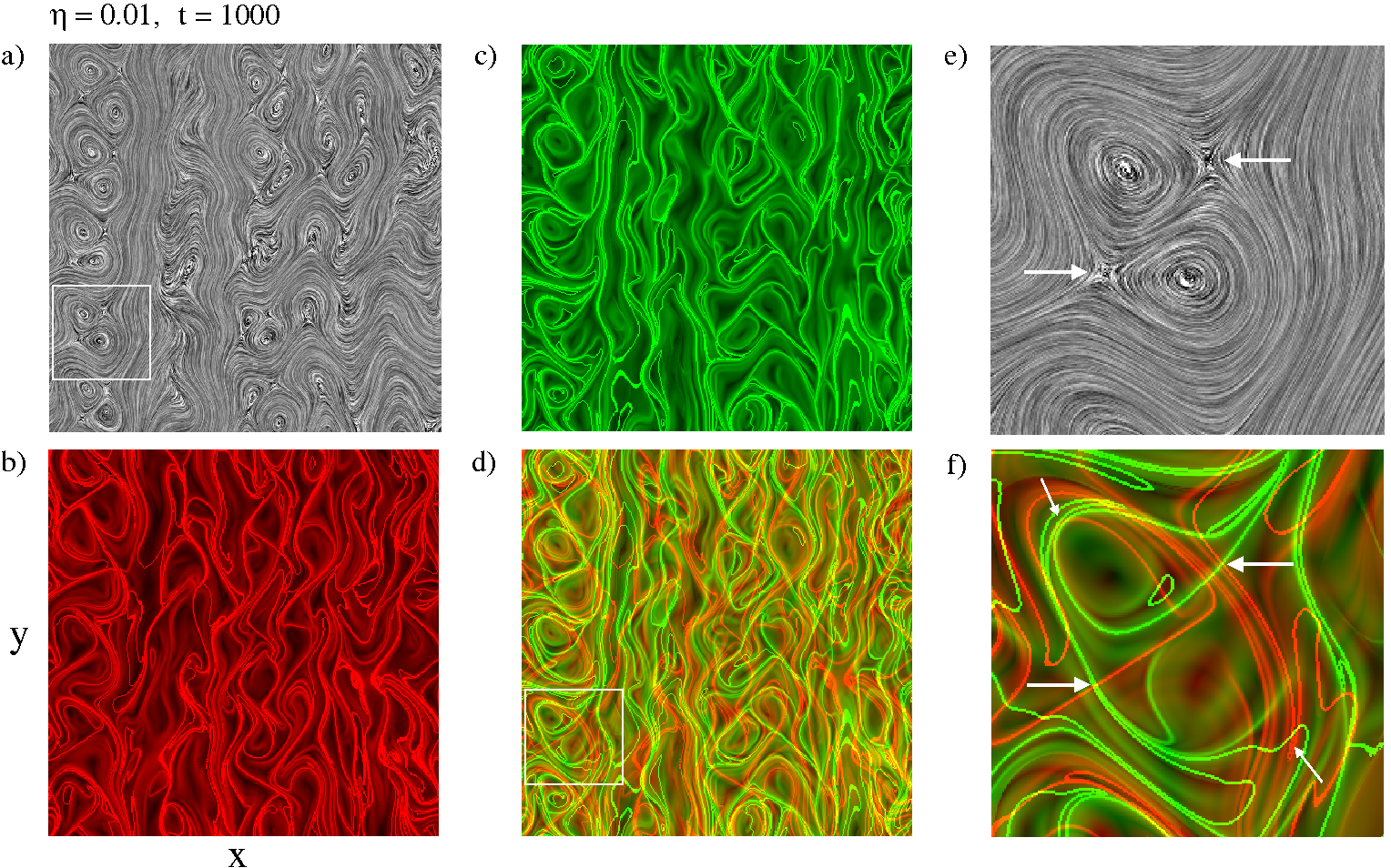
Figure 7: (Color online) (a) Line integral convolution plot showing the streamlines of the $xy$–components of the velocity field at $t=1000$ for $\eta=0.01$; (b) the attracting Lagrangian coherent structures (LCS) (red); (c) the repelling LCS (green); (d) superposition of (b) and (c); (e) enlargement of the square region of (a); (f) enlargement of the square region of (d).

In order to quantify the degree of particle dispersion or chaotic mixing in the flow, Fig. 8 shows the probability distribution functions (PDFs) of the three finite–time Lyapunov exponents for the same state shown in Fig. 7. The PDFs were obtained from a set o $64^{3}$ initial conditions uniformly distributed in the box at $t_{0}=1000$, with $\tau=10$. There is a considerable amount of trajectories with two positive Lyapunov exponents, thus sheet–like magnetic field structures are expected. The broad tails in $\sigma_{1}$ are due to initial conditions that are very close to the repelling material lines, which are regions where the stretching is stronger than the average. On the other hand, the broad tails in negative values of $\sigma_{3}$ reflect contraction in the vicinity of the attracting material lines. Since the flow is weakly compressible, with the Mach number below 0.4, for almost all initial conditions one of the exponents is close to zero. The PDF for $\sigma_{2}$ shows a Gaussian distribution. The overbars on $\sigma$ denote average values.

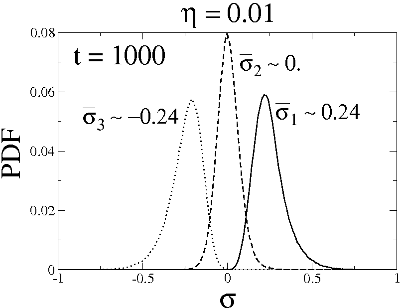
Figure 8: PDFs of the finite–time Lyapunov exponents at $t_{0}=1000$ and $\tau=10$ for $\eta=0.01$.

For $\eta=0.05$ the time series of $B_{\rm rms}$ and $u_{\rm rms}$ are intermittent. To understand the influence of B on u, the FTLE are computed for different initial times marked with vertical lines in Fig. 5. Figure 9 shows the LIC and LCS plots at $t=2100$, just before a burst of magnetic energy in the time series of Fig. 5(b). In comparison to $\eta=0.01$, there seems to be less order in the distribution of vortices in the LIC plot of Fig. 9(a) than in 7(a) and the greater complexity in the distribution of material lines in the LCS plots of Figs. 9(b)–(d) and (f) indicates that transport of passive scalars is enhanced due to the frequent crossings of attracting and repelling lines. This is expected, since $B_{\rm rms}$ is much lower for $\eta=0.05$ and has a smaller impact on the velocity field.

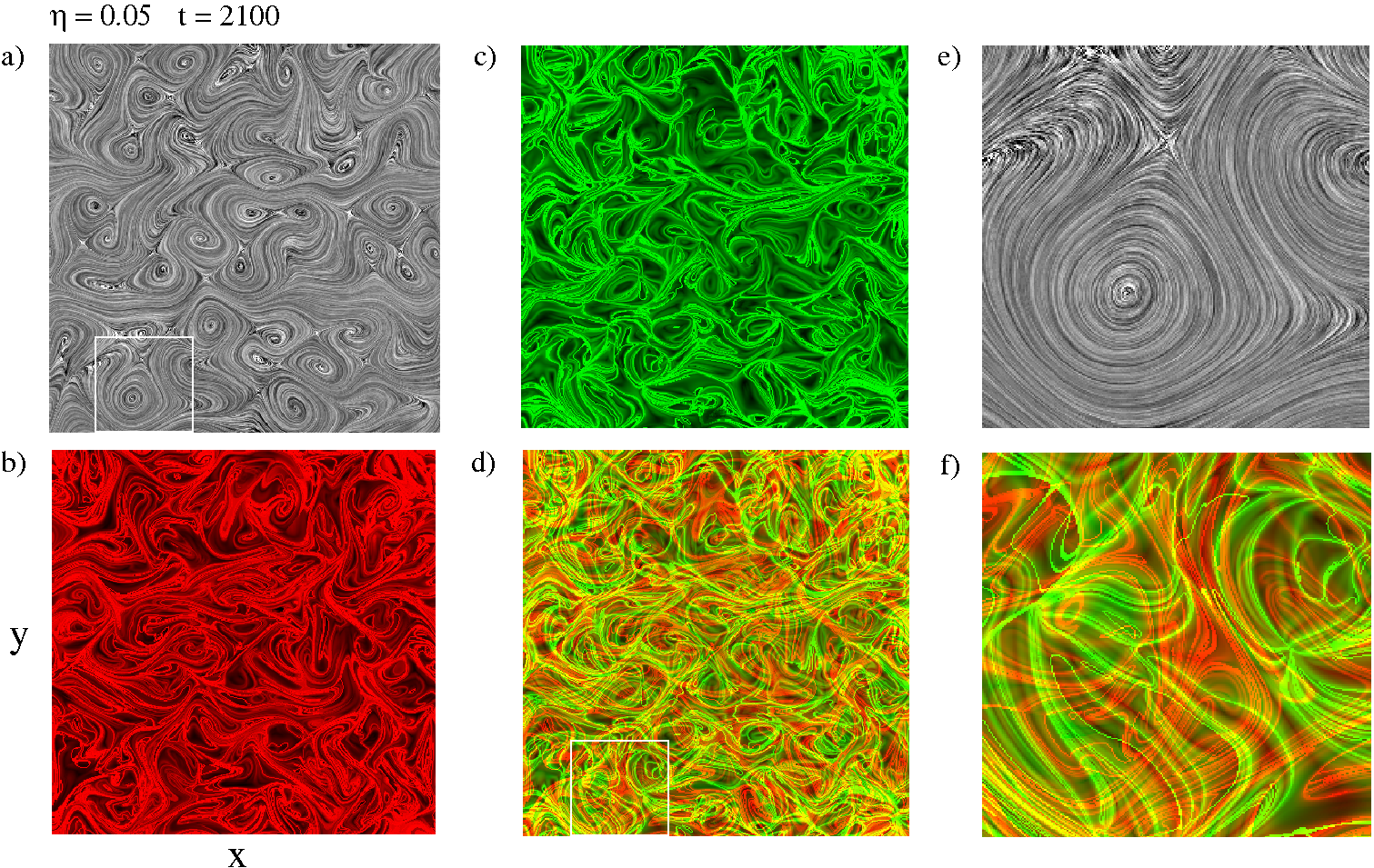
Figure 9: (a) Line integral convolution plot showing the streamlines of the $xy$–components of the velocity field at $t=2100$ for $\eta=0.05$; (b) the attracting Lagrangian coherent structures (LCS) (red); (c) the repelling LCS (green); (d) superposition of (b) and (c); (e) enlargement of the square region of (a); (f) enlargement of the square region of (d).

At $t=2400$ the time series of $B_{\rm rms}$ has a peak of energy burst. As seen in Fig. 10, there is a stronger impact of this magnetic energy release on the velocity field in comparison with t=2100 (Fig. 9). The LIC plot of Fig. 10(a) does not show much difference in relation to Fig. 9(a). However, the LCS plots of Figs. 10(b)–(d) show wider regions of low particle dispersion. This is clearer in Fig. 10(f), which shows an intermediate level of complexity in comparison to Figs. 7(f) and 9(f). Thus, a stronger magnetic field diminishes chaotic mixing in the velocity field, which is measured by the PDFs of the FTLE, shown in Fig. 11.

One can see that the PDFs for the intermittent dynamo (Fig. 11(a),(b)) are wider than for the regular mean–field dynamo (Fig. 8). They also have a larger $\bar{\sigma}_{1}$, revealing that the flow is more chaotic for $\eta=0.05$ than for $\eta=0.01$. Moreover, broader tails in the PDFs of Fig. 11 mean that more intermittency is to be expected in the evolution of passive scalars at $\eta=0.05$. A summary of the results is found in Table 1, which shows $\bar{\sigma}_{1,2,3}$ and their standard deviations for $\eta=0.01$ at $t=1000$ and for $\eta=0.05$ at four values of $t$ representing the beginning and apex of the two magnetic energy bursts indicated in Fig. 5. The mean value $\bar{\sigma}_{1}$ and the standard deviation decrease at both bursts. Figure 12 is a plot of $\bar{\sigma}_{1}$ as a function of $B_{\rm rms}$ using only data from Table 1, which are fitted with the linear equation $\bar{\sigma}_{1}\approx 0.348-0.345B_{\rm rms}$. Although we need more statistics to draw conclusions, our preliminary results suggest that the decay of chaoticity in the velocity field is proportional to $B_{\rm rms}$.

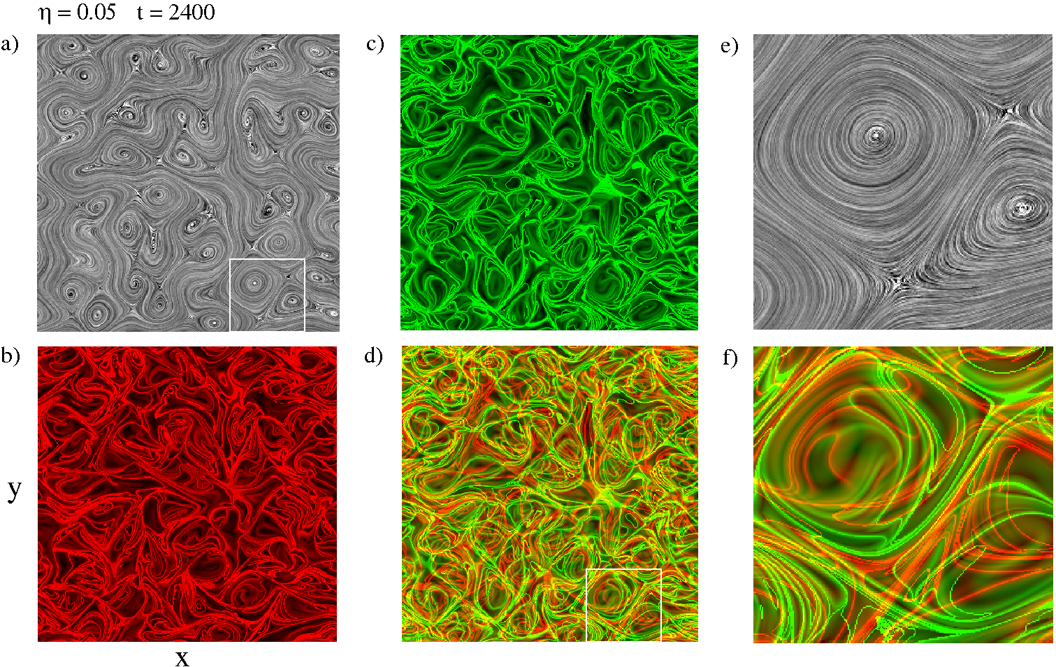
Figure 10: (a) Line integral convolution plot showing the streamlines of the $xy$–components of the velocity field at $t=2400$ for $\eta=0.05$; (b) the attracting Lagrangian coherent structures (LCS) (red); (c) the repelling LCS (green); (d) superposition of (b) and (c); (e) enlargement of the square region of (a); (f) enlargement of the square region of (d).

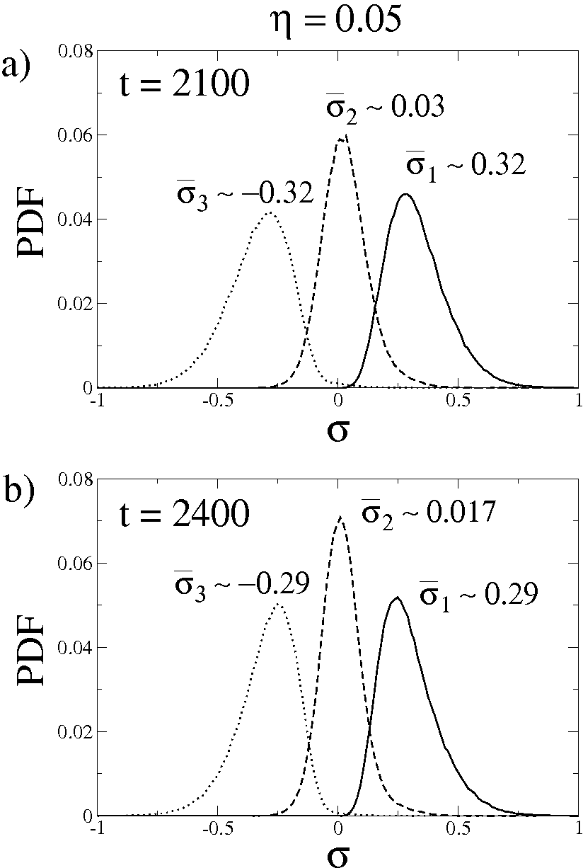
Figure 11: PDFs of the finite–time Lyapunov exponents for $\eta=0.05$ at (a) $t=2100$ and (b) $t=2400$.

Table 1: Mean values and standard deviations of finite–time Lyapunov exponents.

	$\eta=0.01$	$\eta=0.05$
	$t=1000$	$t=2100$	$t=2400$	$t=5600$	$t=6000$
$\bar{\sigma}_{1}$	0.249	0.328	0.298	0.332	0.303
$\bar{\sigma}_{2}$	0.006	0.030	0.017	0.032	0.021
$\bar{\sigma}_{3}$	-0.245	-0.328	-0.292	-0.333	-0.299
std$(\sigma_{1})\quad$	0.096	0.125	0.123	0.125	0.124
std$(\sigma_{2})\quad$	0.067	0.098	0.089	0.098	0.091
std$(\sigma_{3})\quad$	0.098	0.137	0.124	0.138	0.127

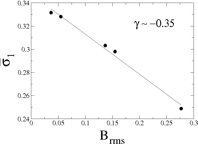
Figure 12: Maximum finite–time Lyapunov exponent of the velocity field $(\bar{\sigma}_{1})$ as a function of $B_{\rm rms}$ using data from Table 1. The fitted line has slope $\gamma\sim-0.345$.

5 Conclusions

We have employed Lagrangian coherent structures (LCS) and the statistics of finite–time Lyapunov exponents (FTLE) to study chaotic stirring in 3–D MHD dynamo simulations with helical forcing. Attracting LCS provide the pathways that are more likely to be followed by passive scalars and their crossings with repelling LCS provide the mechanism for transport between different regions of the fluid. The PDFs of FTLE provide a quantification of chaotic mixing in the flow. We explored the impact of the magnetic field on the velocity field in a saturated nonlinear dynamo and in an intermittent dynamo, and the maximum FTLE was shown to be a linear function of the magnetic energy. The increase in the flow’s chaoticity when the magnetic diffusivity is increased from $\eta=0.01$ to $\eta=0.05$ is the result of the reduction of the effect of the Lorentz force upon the velocity field. Enhanced chaoticity leads to stronger line stretching and field amplification, and the “competition” between this effect and destruction of magnetic flux due to magnetic diffusion seems to be the main cause of the intermittent time series of magnetic energy observed when $\eta=0.05$, which is close to the critical value for dynamo action.

Our analysis has direct applications in astrophysics, where the equipartition–strength magnetic fields observed in planets and stars are thought to be the result of a dynamo process, whereby kinetic energy from the motion of a conducting fluid is converted into magnetic energy [33]. Experimental detection of LCS and computation of FTLE in the solar surface can be performed using velocity fields estimated from observational data. Such estimations can be obtained from digital images using the optical flow algorithm, employed by [34] to extract the velocity field from images of coronal mass ejections obtained with the SOHO LASCO C2 coronagraph. Recently, horizontal velocity fields in the photosphere were inferred from Hinode images [35] and the Swedish Vacuum Solar Telescope [36]. Solar subsurface flows can be inferred from helioseismic data [37], thus LCS can also aid the tracing of particle transport by turbulence in stellar interiors.

References

References

- [1] Lekien F and Coulliette C 2007 Phil. Trans. R. Soc. A 365 3061
- [2] Falkovich G, Gawedzki K and Vergassola M 2001 Rev. Mod. Phys. 73 913
- [3] Rempel E L, Proctor M R E and Chian A C-L 2009 Mon. Not. R. Astron. Soc. 400, 509
- [4] Rempel E L, Chian A C-L and Brandenburg A 2011 Astrophys. J. 735 L9
- [5] Green M A, Rowley C W and Haller G 2007 J. Fluid Mech. 572 111
- [6] Voth G A, Haller G and Gollub J P 2002 Phys. Rev. Lett. 88 254501
- [7] Mathur M, Haller G, Peacock T, Ruppert-Felsot J E and Swinney H L 2007 Phys. Rev. Lett. 98 144502
- [8] Sandulescu M, Lopez C, Hernández-García E and Feudel U 2007 Nonlinear Proc. Geoph. 14 443
- [9] Olascoaga M J, Beron-Vera F J, Brand L E and Kocak H 2008 J. Geophys. Res. 113 C12014
- [10] Tang W, Chan P W and Haller G 2010 CHAOS 20 017502
- [11] Padberg K, Hauff T, Jenko F and Junge O 2007 New J. Phys. 9 400
- [12] Borgogno D, Grasso D, Pegoraro F and Schep T J 2011 Phys. Plasmas 18 102307
- [13] Leoncini X, Agullo O, Muraglia M and Chandre C 2006 Eur. Phys. J. B 53 351
- [14] Childress S and Gilbert A D 1995 Stretch, Twist, Fold: The Fast Dynamo (Berlin: Springer-Verlag)
- [15] Galloway D J and Frisch U 1986 Geophys. Astrophys. Fluid Dyn. 36 53
- [16] Galloway D J and Proctor M R E 1992 Nature 356 691
- [17] Smith S G L, Tobias S M 2004 J. Fluid Mech. 498, 1
- [18] Brandenburg A, Klapper I and Kurths J 1995 Phys. Rev. E 52 R4602
- [19] Cattaneo F, Hughes D W and Kim E-J 1996 Phys. Rev. Lett. 76 2057
- [20] Zienicke E, Politano H and Pouquet A 1998 Phys. Rev. Lett. 81 4640
- [21] Balsara D S, Kim J 2005 Astrophys. J 634 390
- [22] Haller G 2001 Physica D 149 248
- [23] Shadden S C, Lekien F and Marsden J E 2005 Physica D 212 271
- [24] Zel’dovich Ya B, Ruzmaikin A A, Molchanov S A and Sokoloff D D 1984 J. Fluid Mech. 144 1
- [25] Cucitore R, Quadrio M and Baron, A 1999 Eur. J. Mech. B/Fluids 18 261
- [26] Rom–Kedar V and Wiggins S 1990 Arch. Ration. Mech. An. 109 239
- [27] Wiggins S 2005 Annu. Rev. Fluid Mech. 37 295
- [28] Alexakis A, Mininni P D and Pouquet A (2007) New J. Phys. 9, 298
- [29] Moffatt H K 1978 Magnetic field generation in electrically conducting fluids (Cambridge: Cambridge Univ. Press)
- [30] Krause F and Rädler K-H 1980 Mean field magnetohydrodynamics and dynamo theory (Oxford: Pergamon Press)
- [31] Cabral B and Leedom L 1993 Proc. Siggraph, 263 (Anaheim: ACM Press)
- [32] Mathur M et al. 2007 Phys. Rev. Lett. 98 144502
- [33] Brandenburg A and Subramanian K 2005 Phys. Rep. 417 1
- [34] Colaninno R C and Vourlidas A. 2006 Astrophys. J. 652 1747
- [35] Tan C, Chen P F, Abramenko V and Wang H 2009 Astrophys. J. 690 1820
- [36] Getling A V and Buchnov A A 2010Astron. Rep. 50 254
- [37] Woodard M F 2002 Astrophys. J. 565 634