Search for Continuous Gravitational Waves: Optimal StackSlide method at fixed computing cost

Abstract

Coherent wide parameter-space searches for continuous gravitational waves are typically limited in sensitivity by their prohibitive computing cost. Therefore semi-coherent methods (such as StackSlide) can often achieve a better sensitivity. We develop an analytical method for finding optimal StackSlide parameters at fixed computing cost under ideal conditions of gapless data with Gaussian stationary noise. This solution separates two regimes: an unbounded regime, where it is always optimal to use all the data, and a bounded regime with a finite optimal observation time. Our analysis of the sensitivity scaling reveals that both the fine- and coarse-grid mismatches contribute equally to the average StackSlide mismatch, an effect that had been overlooked in previous studies. We discuss various practical examples for the application of this optimization framework, illustrating the potential gains in sensitivity compared to previous searches.

I Introduction

Motivation. The detection of continuous gravitational waves (CWs) from spinning neutron stars (NSs) in our galaxy remains an elusive goal, despite the global network of detectors LIGO Abbott et al. (2009a), Virgo Accadia et al. (2011) and GEO 600 Grote (2010) having completed their initial and enhanced science runs (e.g. see Abadie et al. (2012); Abbott et al. (2010, 2009b); Abadie et al. (2010)). The search for CWs will likely remain a difficult challenge with uncertain prospects even in the era of Advanced detectors Harry (2010); The Virgo Collaboration (2009); Willke et al. (2006) and third-generation detectors such as ET Punturo et al. (2010). Two main reasons for this are (i) astrophysical priors on CWs and (ii) the large parameter space of signal parameters to explore (cf. Prix (2009) for a review and further references).

(i) Current astrophysical priors contain large uncertainties on the expected strength of CW emissions from spinning NSs, with a strong bias towards extremely weak signals, informed by the population of known pulsars as well as by a statistical analysis of a putative galactic “gravitar” population Knispel and Allen (2008). (ii) The required number of templates for a coherent matched-filter search over a range of unknown signal parameters typically grows very rapidly with increasing duration of data analyzed. Therefore only a fraction of the available data can be analyzed coherently (e.g. see Brady et al. (1998); Wette et al. (2008); Abbott et al. (2007)).

It was realized early on Brady and Creighton (2000) that in situations where the total computing cost of the search is constrained, a semi-coherent approach could typically achieve better sensitivity than coherent matched filtering: shorter segments of data are analyzed coherently, then the statistics from these segments are combined incoherently. One method of incoherent combination simply consists of summing the statistics from the different segments, which is typically referred to as the “StackSlide” method in the CW context (also known as the Radon transform). The template bank used for the semi-coherent combination of coherent statistics is referred to as the fine grid, as it typically requires a higher resolution than the template banks of the per-segment coherent searches (referred to as coarse grids). Details of the respective template banks will be discussed in Sec. III.4.

There are a number of different semi-coherent methods: for example, recent work Pletsch (2011) has shown that StackSlide sensitivity can be improved by a sliding coherence-window approach. A closely related variant to StackSlide is the Hough transform Krishnan et al. (2004), which counts the number of segments in which the statistic crosses a given threshold, instead of summing the statistics. This is generally less sensitive, but is designed to be more robust in the presence of strong non-stationarities. A somewhat different semi-coherent approach are cross-correlation methods, described in more detail in Dhurandhar et al. (2008).

Related to the semi-coherent methods are the so-called hierarchical schemes, which consist of following up “promising” candidates from a (coherent or semi-coherent) search by subsequent, more sensitive searches, referred to as “stages”. This procedure is iterated until the parameter space of surviving candidates is sufficiently narrowed down for a fully coherent follow-up using all the data. Work on implementing such schemes in practice is still ongoing.

Optimization problem. In this paper we focus on the standard single-stage StackSlide method, which was also used in previous optimization studies Brady and Creighton (2000); Cutler et al. (2005), and is relatively straightforward to describe analytically.

Any search method contains a number of tuneable parameters, such as the template-bank mismatch, the data selection procedure, and the number and length of segments to analyze. Hierarchical schemes would further require specification of the number of stages and the respective distributions of computing costs and candidate thresholds. The sensitivity of a search generally depends on all these choices, and we therefore need to study how to maximize sensitivity as a function of these parameters.

This optimization problem has been studied previously by Brady and Creighton Brady and Creighton (2000) (henceforth ’BC’) and subsequently by Cutler, Gholami and Krishnan Cutler et al. (2005) (in the following ’CGK’). Both studies have focused on the wider problem of optimizing a multi-stage hierarchical scheme of StackSlide stages, and have directly resorted to fully numerical exploration of the optimization problem. Here instead we focus on the simpler single-stage search, which allows us to fully analytically analyze the problem. In the next step this can be used as a building block to attack the optimization of hierarchical schemes.

Note that for a network of detectors with different noise-floors, the choice of detectors to use at fixed computing cost is part of the optimization problem, but under the present assumption of “ideal data” the answer can be obtained independently Prix (2008). More work is required to develop a practical algorithm to compute the optimal search parameters for given data from a network of detectors, including gaps, non-stationarities and various detector artifacts.

Summary of main results. Careful analysis of the sensitivity scaling shows that the average StackSlide mismatch is given by the sum of the average mismatches from the coarse- and fine-grid template banks, an effect that had previously been overlooked. Note that we allow for independent coarse- and fine-grid mismatches, while BC and CGK forced them to be equal as an ad-hoc constraint.

The analytic optimization is achieved by using local power-law approximations to the computing-cost and sensitivity functions. The results provide analytic self-consistency conditions for the optimal solution: if the initial power-law coefficients agree with those found at the analytic solution, then the solution is self-consistent and (locally) optimal. If this is not the case, one can iterate over successive solutions or scan a range of StackSlide parameters, in order to “bootstrap” into a self-consistent optimal solution.

We find that the analytic solution for StackSlide searches separates two different regimes depending on the power-law coefficients: a bounded regime in which there is a finite optimal observation time, and an unbounded regime in which the optimal solution always consists of using all of the available data, irrespective of the available computing-cost.

Plan of the paper. In Sec. II we discuss the general CW optimization problem, which includes the single-stage StackSlide search as the lowest-level building block. In Sec. III we derive the sensitivity estimate and computing-cost functions for StackSlide searches, and motivate their approximation as local power-laws. After deriving in Sec. IV the general analytical solution and discussing a few special cases, we provide examples for the practical application of this framework in Sec. V: directed searches, all-sky searches, and searches for CWs from NSs in binary systems.

II Maximizing probability of a CW detection

The goal for wide parameter-space CW searches for unknown signals should be to maximize the probability of detection, given current astrophysical priors, detector data, and finite computing resources. Conceptually one can think of this problem as a hierarchy of two questions:

1. What parameter-space $\mathbb{P}\subseteq\mathbb{P}^{(0)}$ to search? More generally: how to distribute the total available computing power $C_{0}$ over the space $\mathbb{P}^{(0)}$ of possible CW signals, given astrophysical priors, detector data and an (optimal) search method?

2. What is the optimal search method? Namely, which method yields the highest detection probability $p_{\mathrm{det}}$ on a parameter-space cell $\Delta\mathbb{P}$ if we spend computing-cost $\Delta C$ on it?

The answer to the first question relies on the second, but we can analyze the lower-level second question independently of the first. There has been surprisingly little work on this problem so far. The first question has hardly been addressed at all, except for recent work by Knispel Knispel (2011). The second question has been studied previously by BC Brady and Creighton (2000) and CGK Cutler et al. (2005), assuming a specific type of hierarchical scheme, which we refer to as the classical hierarchical scheme (CHS).

In the CHS one performs a hierarchy of semi-coherent searches (called stages), starting with a relatively low-sensitivity search over the whole initial parameter space $\mathbb{P}^{(1)}$. Promising candidates crossing the first-stage threshold are selected and constitute the search subspace $\mathbb{P}^{(2)}\subset\mathbb{P}^{(1)}$ for the second, higher-sensitivity stage. This is iterated until eventually after $m$ such stages a fully-coherent search over all the data can be performed on the surviving candidates. At this point one has reached the maximal possible sensitivity for a small portion $\mathbb{P}^{(m)}\subset\mathbb{P}^{(1)}$ of the initial parameter space.

Each stage ${(i)}$ is characterized by its input parameter-space $\mathbb{P}^{(i)}$, a computing-cost constraint $C_{0}^{(i)}$ and a false-alarm probability $p_{\mathrm{fA}}^{(i)}$. Each stage selects a candidate subspace $\mathbb{P}^{(i+1)}\subset\mathbb{P}^{(i)}$ to follow up in the next stage. An optimal per-stage search would result in the highest detection probability $p_{\mathrm{det}}^{(i)}$ for given signal strength $h_{\mathrm{rms}}$ and constraints $\{p_{\mathrm{fA}}^{(i)},\,\mathbb{P}^{(i)},\,C_{0}^{(i)}\}$. The tuneable CHS parameters are therefore the number $m$ of stages and the per-stage constraints $\{p_{\mathrm{fA}}^{(i)},C_{0}^{(i)}\}$. These can be varied in order to maximize the overall detection probability $p_{\mathrm{det}}(h_{\mathrm{rms}})$ for the given total signal parameter-space $\mathbb{P}^{(0)}$, computing cost $C_{0}=\sum_{i=1}^{m}C_{0}^{(i)}$ and false-alarm probability $p_{\mathrm{fA}}=\prod_{i=1}^{m}\,p_{\mathrm{fA}}^{(i)}$.

This formulation of the CHS suggests that each stage ${(i)}$ could be considered an independent optimization problem for given external constraints $\{p_{\mathrm{fA}}^{(i)},\mathbb{P}^{(i)},C_{0}^{(i)}\}$, if none of its internal parameters interfere with the overall hierarchical scheme. One might contend that the parameter-space resolution of the search violates this clean factorization: the follow-up space $\mathbb{P}^{(i+1)}$ from stage ${(i)}$ depends on its parameter-space resolution, which might impact the required computing-cost of the next stage. However, it is easy to see that (to first order) such a coupling is not expected. The number of candidates $\mathcal{N}_{\mathrm{cand}}$ returned from any stage (except for the last one) will be dominated by the number $\mathcal{N}_{\mathrm{fA}}$ of false alarms. Therefore $\mathcal{N}_{\mathrm{cand}}\approx\mathcal{N}_{\mathrm{fA}}\approx p_{\mathrm{fA}}\,\mathcal{N}$, where $\mathcal{N}$ is the number of (approximately) independent templates searched in this stage. This can be estimated as $\mathcal{N}\approx V_{\mathbb{P}}/v_{0}$, in terms of the (metric) volume $V_{\mathbb{P}}$ of the parameter space $\mathbb{P}$, and the volume $v_{0}$ covered by one template. Therefore the number $\mathcal{N}_{\mathrm{cand}}$ of follow-up candidates from any stage does indeed depend on its parameter-space resolution, which depends on the internal stage parameters. However, the computing cost of the next stage depends primarily on the volume of the follow-up parameter-space, which is $V_{\mathrm{fA}}\approx\mathcal{N}_{\mathrm{fA}}\,v_{0}\approx p_{\mathrm{fA}}\,V_{\mathbb{P}}$, and is therefore independent of internal stage parameters. It is interesting to note that each stage ${(i)}$ in this scheme achieves a reduction of the input parameter-space volume by roughly a factor of the false-alarm probability $p_{\mathrm{fA}}^{(i)}$, irrespective of the internal details of that search.

The optimal per-stage search method is essentially unknown, but following BC and CGK we focus on a known good strategy, namely the StackSlide method. While different semi-coherent methods differ in the details and their exact sensitivity, they share the main characteristics of coherently searching $N$ shorter segments of length $\Delta T$, and combining them incoherently in some way. We roughly expect the sensitivity per cost of different methods to behave qualitatively similarly to the StackSlide method, but more work would be required to study this in detail.

III Properties of a single-stage StackSlide search

The general StackSlide scheme consists of dividing the data (of total duration $T$) into $N$ segments of duration $\Delta T=T/N$, then performing a coherent matched-filter search on each segment and combining these statistics incoherently to a new statistic $\Sigma$ by summing them across segments. The coherent matched-filter statistic used is the $\mathcal{F}$-statistic, which was first derived in Jaranowski et al. (1998) and extended to multiple detectors in Cutler and Schutz (2005). Using the same amount of data as a fully coherent search, the resulting semi-coherent statistic is less sensitive, but substantially cheaper to compute over a wide parameter space. At fixed computing cost a semi-coherent search is therefore generally more sensitive than a fully coherent $\mathcal{F}$-statistic search.

Notation: we distinguish quantities $Q$ that can refer to either the coherent or the incoherent step in the following way: we use a tilde, i.e. $\widetilde{Q}$ when referring to the coherent step, and a hat, i.e. $\widehat{Q}$ when referring to the incoherent step. For the following derivations we restrict ourselves to a single-detector formalism for simplicity, but we state the (trivial) generalization to $N_{\mathrm{det}}\geq 1$ detectors of relevant results.

III.1 The StackSlide search method

Let $k=1\ldots N$ be the index over segments, and $\lambda\in\mathbb{P}$ a point in the search space $\mathbb{P}$ of signal parameters. The “ideal” StackSlide statistic $\Sigma_{0}(\lambda)$ is defined as

$$\Sigma_{0}(\lambda)\equiv\sum_{k=1}^{N}2\mathcal{F}_{k}(\lambda)\,,$$ (1)

i.e. a simple sum of $\mathcal{F}$-statistic values $\{2\mathcal{F}_{k}(\lambda)\}_{k=1}^{N}$ computed at the same template point $\lambda$ across all $N$ segments.

This would require computing the $\mathcal{F}$-statistic over the same template bank as $\Sigma_{0}$ in every segment. However, the metric resolution of $\Sigma_{0}$ is generally finer than that of the single-segment $\mathcal{F}$-statistics Pletsch (2010), and therefore this approach would spend unnecessary computing cost on the coherent $\mathcal{F}$-statistic. In practice $\mathcal{F}$ is therefore computed over a coarse grid of $\widetilde{\mathcal{N}}$ templates in each segment $k$, and is interpolated in order to sum $\mathcal{F}$ on the fine grid of $\widehat{\mathcal{N}}\geq\widetilde{\mathcal{N}}$ templates (e.g. see Pletsch and Allen (2009)).

Typically the interpolation consists of picking the closest (in the metric sense) coarse-grid point $\widetilde{\lambda}_{k}(\widehat{\lambda})$ to the fine-grid point $\widehat{\lambda}$ from every segment $k$, i.e. we approximate Eq. (1) by

$$\Sigma(\widehat{\lambda})\equiv\sum_{k=1}^{N}2\mathcal{F}_{k}\left(\widetilde{\lambda}_{k}(\widehat{\lambda})\right)\approx\Sigma_{0}(\widehat{\lambda})\,,$$ (2)

which we refer to as the “interpolating” StackSlide statistic $\Sigma$. The following sensitivity optimization focuses exclusively on this interpolating StackSlide method, which is the most relevant approach for current practical applications. The subtle difference between interpolating StackSlide $\Sigma$ and ideal StackSlide $\Sigma_{0}$ with respect to its sensitivity and mismatches has been overlooked in previous studies, and will be important for the optimization problem.

III.2 Mismatch and metric

III.2.1 $\mathcal{F}$-statistic mismatch

In the presence of a signal timeseries $s(t,\lambda_{\mathrm{s}})$ with phase parameters $\lambda_{\mathrm{s}}$, the statistic $2\mathcal{F}_{k}(\widetilde{\lambda})$ in a point $\widetilde{\lambda}$ follows a non-central $\chi^{2}$-distribution with four degrees of freedom and non-centrality parameter $\rho_{k}^{2}(\lambda_{\mathrm{s}},\widetilde{\lambda})$. We denote this probability distribution as

$$P\left(2\mathcal{F}_{k}|\rho_{k}^{2}\right)=\chi^{2}_{4}(2\mathcal{F}_{k};\rho_{k}^{2})\,,$$ (3)

which has the expectation value

$$E\left[2\mathcal{F}_{k}(\lambda_{\mathrm{s}},\widetilde{\lambda})\right]=4+\rho_{k}^{2}(\lambda_{\mathrm{s}},\widetilde{\lambda})\,.$$ (4)

The quantity $\rho_{k}$ is often referred to as the coherent signal-to-noise ratio (SNR). In the case of a perfectly-matched template $\widetilde{\lambda}=\lambda_{\mathrm{s}}$, the resulting “optimal” SNR Jaranowski et al. (1998) in segment $k$ can be expressed as

$$\rho_{k}^{2}(\lambda_{\mathrm{s}},\lambda_{\mathrm{s}}) =\frac{2}{S_{\mathrm{n}}}\int_{t_{k}}^{{t_{k}}+\Delta T}s^{2}(t,\lambda_{\mathrm{s}})\,dt$$

$$\equiv\frac{2}{S_{\mathrm{n}}}\,h_{\mathrm{rms},k}^{2}\,\Delta T\,,$$ (5)

where $t_{k}$ is the start-time of the $k$th segment, $S_{\mathrm{n}}$ is the (single-sided) noise power spectral density at the signal frequency $f_{\mathrm{s}}$. In the second equality we defined the rms signal strength $h_{\mathrm{rms},k}$ Cutler et al. (2005) in segment $k$, which is a useful measure of the intrinsic signal strength in the detectors, independently of the quality and the amount of data used.

The signal strength $h_{\mathrm{rms},k}$ depends on the intrinsic signal amplitude $h_{0}$, the sky-position, polarization angles, and detector orientation during segment $k$. One can show Jaranowski et al. (1998); Prix (2010) that averaging $h_{\mathrm{rms},k}^{2}$ isotropically over sky-positions and polarization angles yields the relation $\langle h_{\mathrm{rms},k}^{2}\rangle_{\mathrm{sky,pol}}=(2/25)\,h_{0}^{2}$. Furthermore, for segment lengths of order $\Delta T\gtrsim\mathcal{O}\left(1\,\mathrm{days}\right)$, the averaging in Eq. (5) results in $h_{\mathrm{rms},k}$ tending towards a constant over all segments. Therefore it will be convenient to approximate $h_{\mathrm{rms},k}\approx h_{\mathrm{rms}}$, and so we can write

$$\rho_{k}^{2}(\lambda_{\mathrm{s}},\lambda_{\mathrm{s}})\approx\frac{2}{S_{\mathrm{n}}}h_{\mathrm{rms}}^{2}\,\Delta T\equiv\rho_{\mathrm{opt}}^{2}(\Delta T)\,,$$ (6)

which defines the average optimal SNR $\rho_{\mathrm{opt}}$ for given segment length $\Delta T$.

Note that this approximation only applies to the perfectly-matched SNR $\rho_{k}(\lambda_{\mathrm{s}},\lambda_{\mathrm{s}})$. The “mismatched” SNR $\rho_{k}(\lambda_{\mathrm{s}},\widetilde{\lambda})$ in an offset template $\widetilde{\lambda}=\lambda_{\mathrm{s}}+\Delta\lambda$ is reduced with respect to the optimal SNR $\rho_{\mathrm{opt}}(\Delta T)$. The corresponding relative loss defines the (segment-specific) mismatch function $\widetilde{\mu}_{k}(\lambda_{\mathrm{s}},\widetilde{\lambda})$, namely

$$\widetilde{\mu}_{k}(\lambda_{\mathrm{s}},\widetilde{\lambda}) \equiv 1-\frac{\rho_{k}^{2}(\lambda_{\mathrm{s}},\widetilde{\lambda})}{\rho_{\mathrm{opt}}^{2}(\Delta T)}$$

$$=\widetilde{g}_{ij,k}(\lambda_{\mathrm{s}})\,\Delta\lambda^{i}\,\Delta\lambda^{j}+\mathcal{O}\left(\Delta\lambda^{3}\right)\,,$$ (7)

where Taylor-expansion for small offsets $\Delta\lambda$ defines the (coherent) metric tensor $\widetilde{g}_{ij,k}(\lambda)$ for segment $k$. The concept of the parameter-space metric was first introduced in Balasubramanian et al. (1996); Owen (1996), and analyzed in the context of a simplified CW statistic Brady et al. (1998) and the $\mathcal{F}$-statistic Prix (2007a).

The per-segment coarse-grid template bank is constructed under the constraint that no signal point $\lambda_{\mathrm{s}}\in\mathbb{P}$ should exceed a given maximal mismatch $\widetilde{m}$ to its closest (i.e. with the smallest mismatch) coarse-grid template $\widetilde{\lambda}_{k}(\lambda_{\mathrm{s}})$, namely

$$\widetilde{\mu}_{k}\left(\lambda_{\mathrm{s}},\widetilde{\lambda}_{k}(\lambda_{\mathrm{s}})\right)\leq\widetilde{m}\,\quad\mbox{for all}\quad\lambda_{\mathrm{s}}\in\mathbb{P}\,.$$ (8)

III.2.2 Mismatch of “ideal” StackSlide

The “ideal” StackSlide statistic $\Sigma_{0}$ defined in Eq. (1) is the basis for the definition of the semi-coherent metric Brady and Creighton (2000); Pletsch (2010); Messenger (2011)). The statistic $\Sigma_{0}$ follows a non-central $\chi^{2}$-distribution with $4N$ degrees of freedom, denoted as

$$P\left(\Sigma_{0}|\rho_{\Sigma_{0}}^{2}\right)=\chi^{2}_{4N}(\Sigma_{0};\rho_{\Sigma_{0}}^{2})\,,$$ (9)

with non-centrality parameter

$$\rho_{\Sigma_{0}}^{2}(\lambda_{\mathrm{s}},\widehat{\lambda})\equiv\sum_{k=1}^{N}\rho_{k}^{2}(\lambda_{\mathrm{s}},\widehat{\lambda})\,,$$ (10)

where $\lambda_{\mathrm{s}}$ are the signal parameters and $\widehat{\lambda}$ is the location of a fine-grid template. The corresponding expectation value is

$$E\left[\Sigma_{0}(\lambda_{\mathrm{s}},\widehat{\lambda})\right]=4N+\rho_{\Sigma_{0}}^{2}\,.$$ (11)

The perfectly-matched non-centrality parameter $\rho_{\Sigma_{0}}^{2}(\lambda_{\mathrm{s}},\lambda_{\mathrm{s}})$ can be expressed as

$$\rho_{\Sigma_{0}}^{2}(\lambda_{\mathrm{s}},\lambda_{\mathrm{s}}) =\sum_{k=1}^{N}\rho_{k}^{2}(\lambda_{\mathrm{s}},\lambda_{\mathrm{s}})$$

$$=N\rho_{\mathrm{opt}}^{2}(\Delta T)$$

$$=\rho_{\mathrm{opt}}^{2}(T)\,,$$ (12)

which is identical to that of a perfectly-matched $\mathcal{F}$-statistic over the same total duration $T$, as seen from Eq. (6). The reason why the StackSlide statistic $\Sigma_{0}$ is less sensitive than the $\mathcal{F}$-statistic for the same amount of data $T$ stems from the different degrees of freedom of the respective distributions, namely $\chi^{2}_{4}(\rho^{2})$ for the $\mathcal{F}$-statistic as opposed to $\chi^{2}_{4N}(\rho^{2})$ for StackSlide $\Sigma_{0}$.

The mismatch function $\widehat{\mu}_{0}(\lambda_{\mathrm{s}},\widehat{\lambda})$ of ideal StackSlide is defined in analogy to Eq. (7) as

$$\widehat{\mu}_{0}(\lambda_{\mathrm{s}},\widehat{\lambda}) \equiv 1-\frac{\rho_{\Sigma_{0}}^{2}(\lambda_{\mathrm{s}},\widehat{\lambda})}{\rho_{\mathrm{opt}}^{2}(T)}$$

$$=\widehat{g}_{ij}(\lambda_{\mathrm{s}})\,\Delta\lambda^{i}\,\Delta\lambda^{j}+\mathcal{O}\left(\Delta\lambda^{3}\right)\,,$$ (13)

where $\Delta\lambda\equiv\widehat{\lambda}-\lambda_{\mathrm{s}}$ is the offset between the fine-grid template $\widehat{\lambda}$ and the signal location $\lambda_{\mathrm{s}}$, and Taylor-expansion in small $\Delta\lambda$ defines the (semi-coherent) metric tensor $\widehat{g}_{ij}$. Using Eqs. (12) and (7), we can rearrange the expression for the mismatch as

$$\widehat{\mu}_{0}(\lambda_{\mathrm{s}},\widehat{\lambda}) =\frac{1}{N}\sum_{k=1}^{N}\widetilde{\mu}_{k}(\lambda_{\mathrm{s}},\widehat{\lambda})$$

$$\approx\left(\frac{1}{N}\sum_{k=1}^{N}\widetilde{g}_{ij,k}(\lambda_{\mathrm{s}})\right)\,\Delta\lambda^{i}\Delta\lambda^{j}\,,$$ (14)

which shows that the ideal StackSlide mismatch $\widehat{\mu}_{0}$ and metric $\widehat{g}_{ij}$ are segment-averages of the coherent mismatches and metrics, respectively.

The fine-grid template bank of a StackSlide search is constructed under the constraint that no signal point $\lambda_{\mathrm{s}}\in\mathbb{P}$ should exceed a given maximal mismatch $\widehat{m}$ to its closest (i.e. with the smallest mismatch) fine-grid template $\widehat{\lambda}(\lambda_{\mathrm{s}})$, namely

$$\widehat{\mu}_{0}\left(\lambda_{\mathrm{s}},\,\widehat{\lambda}(\lambda_{\mathrm{s}})\right)\leq\widehat{m}\,\quad\mbox{for all}\quad\lambda_{\mathrm{s}}\in\mathbb{P}\,.$$ (15)

III.2.3 Mismatch of “interpolating” StackSlide

We can now combine the above results to derive the mismatch of the interpolating StackSlide statistic $\Sigma$ defined in Eq. (2). This statistic follows a non-central $\chi^{2}_{4N}$ distribution, namely

$$P\left(\Sigma|\rho_{\Sigma}^{2}\right)=\chi^{2}_{4N}(\Sigma;\rho_{\Sigma}^{2})\,,$$ (16)

with non-centrality parameter

$$\rho_{\Sigma}^{2}(\lambda_{\mathrm{s}},\widehat{\lambda})\equiv\sum_{k=1}^{N}\rho_{k}^{2}\left(\lambda_{\mathrm{s}},\widetilde{\lambda}_{k}(\widehat{\lambda})\right)\,,$$ (17)

where $\lambda_{\mathrm{s}}$ are the signal phase parameters, and $\widetilde{\lambda}_{k}(\widehat{\lambda})$ is the closest coarse-grid template in segment $k$ to the fine-grid point $\widehat{\lambda}$.

The mismatch function $\widehat{\mu}(\lambda_{\mathrm{s}},\widehat{\lambda})$ of interpolating StackSlide is therefore

$$\widehat{\mu}(\lambda_{\mathrm{s}},\widehat{\lambda}) \equiv 1-\frac{\rho_{\Sigma}^{2}(\lambda_{\mathrm{s}},\widehat{\lambda})}{\rho_{\mathrm{opt}}^{2}(T)}$$

$$=\frac{1}{N}\sum_{k=1}^{N}\widetilde{\mu}_{k}\left(\lambda_{\mathrm{s}},\,\widetilde{\lambda}_{k}(\widehat{\lambda})\right)\,,$$ (18)

which allows us to express the mismatched non-centrality parameter as

$$\rho_{\Sigma}^{2}(\lambda_{\mathrm{s}},\widehat{\lambda})=\left(1-\widehat{\mu}(\lambda_{\mathrm{s}},\widehat{\lambda})\right)\,\rho_{\mathrm{opt}}^{2}(T)\,.$$ (19)

The extra offset per-segment, $\delta\lambda_{k}\equiv\widetilde{\lambda}_{k}(\widehat{\lambda})-\widehat{\lambda}$, incurred due to using the closest coarse-grid point $\widetilde{\lambda}_{k}(\widehat{\lambda})$ instead of the fine-grid point $\widehat{\lambda}$ tends to increase the mismatch with respect to the ideal mismatch function $\widehat{\mu}_{0}$ of Eq. (14). In order to quantify this effect, we write the effective per-segment offset from a signal as $\Delta\widetilde{\lambda}_{k}\equiv\widetilde{\lambda}_{k}(\widehat{\lambda})-\lambda_{\mathrm{s}}$, while the ideal per-segment offset would be $\Delta\widehat{\lambda}\equiv\widehat{\lambda}-\lambda_{\mathrm{s}}$. We can write $\Delta\widetilde{\lambda}_{k}=\Delta\widehat{\lambda}+\delta\lambda_{k}$, and inserting this into the coherent-metric of Eq. (7) we obtain (neglecting higher-order terms $\mathcal{O}\left(\Delta\lambda^{3}\right)$):

$$\widetilde{\mu}_{k}\left(\lambda_{\mathrm{s}},\widetilde{\lambda}_{k}(\widehat{\lambda})\right)=\widetilde{g}_{ij,k}\,\Delta\widetilde{\lambda}_{k}^{i}\Delta\widetilde{\lambda}_{k}^{j}\\ =\widetilde{\mu}_{k}(\lambda_{\mathrm{s}},\widehat{\lambda})+\widetilde{g}_{ij,k}\,\delta\lambda_{k}^{i}\,\delta\lambda_{k}^{j}+2\widetilde{g}_{ij,k}\,\Delta\widehat{\lambda}^{i}\,\delta\lambda_{k}^{j}\,,$$ (20)

where in the first term we recover the ideal per-segment mismatch function of Eq. (14), the second term represents an extra mismatch due to the offset $\delta\lambda_{k}$, while the last term depends on the opening angle $\theta_{k}$ of the mismatch triangle (see Fig. 1), namely $2|\Delta\widehat{\lambda}||\delta\lambda_{k}|\cos\theta_{k}$, with mismatch norm defined as $|x|^{2}\equiv\widetilde{g}_{ij,k}\,x^{i}x^{j}$.

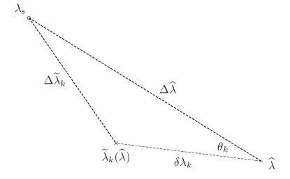
Figure 1: Mismatch triangle formed by the signal point $\lambda_{\mathrm{s}}$, closest fine-grid template $\widehat{\lambda}$, and the coarse-grid template $\widetilde{\lambda}_{k}(\widehat{\lambda})$ closest to $\widehat{\lambda}$ in segment $k$.

We assume that the fine-grid point $\widehat{\lambda}$ falls randomly into the Wigner-Seitz cell of the closest coarse-grid template $\widetilde{\lambda}_{k}(\widehat{\lambda})$ in segment $k$. Given that the coarse-grid metric $\widetilde{g}_{ij,k}$ generally varies across segments, we further assume that the offset $\delta\lambda_{k}$ approximates a uniform random sampling of the coarse-grid Wigner-Seitz cell. Inserting Eq. (20) into (18), we see that the average over the angle-term $|\Delta\widehat{\lambda}||\delta\lambda_{k}|\cos\theta_{k}$ will tend to zero, as any sign of $\cos\theta_{k}$ is equally likely, while the average norm $|\delta\lambda_{k}|^{2}$ will tend to the average mismatch $\left\langle\widetilde{\mu}\right\rangle$ of the coarse-grid template bank, and so we obtain

$$\widehat{\mu}(\lambda_{\mathrm{s}},\widehat{\lambda})\approx\widehat{\mu}_{0}(\lambda_{\mathrm{s}},\widehat{\lambda})+\left\langle\widetilde{\mu}\right\rangle\,.$$ (21)

When estimating the sensitivity of the interpolating StackSlide statistic, we will further average this expression over randomly-chosen signal locations $\lambda_{\mathrm{s}}$, and therefore the above approximate averaging expressions will become exact, and we obtain

$$\left\langle\widehat{\mu}\right\rangle=\left\langle\widehat{\mu}_{0}\right\rangle+\left\langle\widetilde{\mu}\right\rangle\,,$$ (22)

where averaging is performed over the coarse- and fine-grid template banks (i.e. the respective Wigner-Seitz cells).

The probability distribution of signal mismatches in a given template bank constructed with a certain maximal mismatch $m$ depends on the structure and dimensionality of the template bank. The corresponding average mismatch can be expressed as $\left\langle\mu\right\rangle=\xi\,m$, where $\xi\in(0,1)$ is a characteristic geometric factor of the template bank. Such mismatch distributions were studied quantitatively, for example in Messenger et al. (2009). For hyper-cubic lattices, the geometric relation is well known to be exactly $\left\langle\mu\right\rangle=m/3$, which was used in previous optimization studies Brady and Creighton (2000); Cutler et al. (2005). For the more efficient $A_{n}^{*}$-lattices this geometric factor is approximately $\xi\approx 0.5-0.6$ for low dimensions $n\lesssim 6$. Here we allow for general geometric factors $\xi$, but for simplicity we assume it to be identical for the fine- and coarse-grid template banks, and so Eq. (22) can be written as

$$\left\langle\widehat{\mu}\right\rangle=\xi(\widehat{m}+\widetilde{m})\,,\quad\mbox{with}\quad\xi\in(0,1)\,,$$ (23)

where $\widehat{m}$ and $\widetilde{m}$ are the maximal mismatch parameters of fine- and coarse-grid template banks, respectively.

Averaging the non-centrality parameter $\rho_{\Sigma}^{2}$ of Eq. (19) over random signal parameters $\lambda_{\mathrm{s}}$ at fixed signal strength $h_{\mathrm{rms}}$, we can now obtain the expression

$$\left\langle\rho_{\Sigma}^{2}\right\rangle=\left[1-\xi(\widehat{m}+\widetilde{m})\right]\,\frac{2N_{\mathrm{det}}}{S_{\mathrm{n}}}\,h_{\mathrm{rms}}^{2}\,T\,,$$ (24)

where we (trivially) generalized the result to the case of a network of $N_{\mathrm{det}}$ detectors. In this case $S_{\mathrm{n}}$ refers to the harmonic mean over individual-detector PSDs, and $h_{\mathrm{rms}}$ is a noise-weighted average over rms-amplitudes from different detectors (e.g. see Prix (2010)). The fact that both the coarse- and fine-grid mismatches enter this expression has been overlooked in previous studies Brady and Creighton (2000); Cutler et al. (2005), where only the fine-grid mismatch $\widehat{m}$ had been included.

III.3 Sensitivity estimate

The false-alarm and false-dismissal probabilities for a given threshold $\Sigma_{\mathrm{th}}$ of the StackSlide statistic $\Sigma$ of Eq. (2) are

$$p_{\mathrm{fA}}(\Sigma_{\mathrm{th}}) =\int_{\Sigma_{\mathrm{th}}}^{\infty}\chi^{2}_{4N}(\Sigma;0)\,d\Sigma\,,$$ (25)

$$p_{\mathrm{fD}}(\Sigma_{\mathrm{th}},\rho_{\Sigma}^{2}) =\int_{-\infty}^{\Sigma_{\mathrm{th}}}\chi^{2}_{4N}(\Sigma;\rho_{\Sigma}^{2})\,d\Sigma\,,$$ (26)

where the special case of a coherent $\mathcal{F}$-statistic search corresponds to $N=1$.

Sensitivity is often quantified in terms of the weakest (rms-) signal strength $h_{\mathrm{th}}$ required to obtain a given detection probability $p_{\mathrm{det}}^{*}=1-p_{\mathrm{fD}}^{*}$ at a given false-alarm probability $p_{\mathrm{fA}}^{*}$. This requires inverting Eq. (25) to obtain the critical threshold $\Sigma_{\mathrm{th}}^{*}=\Sigma_{\mathrm{th}}(p_{\mathrm{fA}}^{*})$, then substituting this into Eq. (26) and inverting to find the critical non-centrality parameter

$$\rho_{\Sigma}^{*2}=\rho_{\Sigma}^{2}(p_{\mathrm{fA}}^{*},p_{\mathrm{fD}}^{*},N)\,.$$ (27)

The signal location $\lambda_{\mathrm{s}}$ is generally unknown, therefore the mismatch $\widehat{\mu}(\lambda_{\mathrm{s}},\widehat{\lambda})$ of the closest template $\widehat{\lambda}$ and the corresponding mismatched non-centrality parameter $\rho_{\Sigma}^{2}(\lambda_{\mathrm{s}},\widehat{\lambda})$ of Eq. (19) follow a random distribution. In order to estimate the threshold rms signal strength $h_{\mathrm{th}}$, one would have to compute $p_{\mathrm{fD}}(p_{\mathrm{fA}}^{*},h_{\mathrm{th}})$ by averaging the right-hand side of Eq. (26) over the (known) mismatch distribution of $\widehat{\mu}$. Furthermore, for statements about physical upper limits and sensitivity of a given search pipeline, it is often required to quantify the sensitivity in terms of the intrinsic GW amplitude $h_{0}$, instead of the rms detector strain $h_{\mathrm{rms}}$, which would require further averaging of Eq. (26) over the (potentially) unknown sky-position and polarization parameters. This problem has recently been studied in detail in Wette (2012).

For our present purpose it will be sufficient to obtain the correct scaling of sensitivity with StackSlide parameters $\{N,T,\widetilde{m},\widehat{m}\}$, while the absolute sensitivity level is less important. We will therefore employ the usual simplification of this problem, which consists in averaging $\rho_{\Sigma}^{2}$ instead of $p_{\mathrm{fD}}(\rho_{\Sigma}^{2})$ over the mismatch distribution of $\widehat{\mu}$, so we approximate

$$p_{\mathrm{fD}}(p_{\mathrm{fA}}^{*},h_{\mathrm{th}}) =\left\langle\left.p_{\mathrm{fD}}(p_{\mathrm{fA}}^{*},\rho_{\Sigma}^{2})\right|_{h_{\mathrm{th}}}\right\rangle_{\lambda_{\mathrm{s}}}$$

$$\approx p_{\mathrm{fD}}\left(p_{\mathrm{fA}}^{*},\left\langle\rho_{\Sigma}^{2}\right\rangle_{\lambda_{\mathrm{s}}}\right)\,.$$ (28)

The results of Wette (2012) indicate that this indeed approximately preserves the scaling of sensitivity as a function of StackSlide parameters.

We can now use Eq. (24) to translate the critical non-centrality parameter $\rho_{\Sigma}^{*2}$ of Eq. (27) into a threshold rms signal-strength $h_{\mathrm{th}}$, namely

$$h_{\mathrm{th}}^{-2}=\frac{2N_{\mathrm{det}}}{\rho_{\Sigma}^{*2}}\,\left[1-\xi(\widehat{m}+\widetilde{m})\right]\,\frac{T}{S_{\mathrm{n}}}\,.$$ (29)

Following the Neyman-Pearson criterion we want to maximize detection probability $p_{\mathrm{det}}^{*}=1-p_{\mathrm{fD}}^{*}$ at fixed false-alarm probability $p_{\mathrm{fA}}^{*}$ and at fixed signal strength $h_{\mathrm{rms}}$. Equivalently we can fix the false-alarm and false-dismissal probabilities and minimize the required threshold rms signal strength $h_{\mathrm{th}}$, which is the traditional optimization approach used in previous studies Brady and Creighton (2000); Cutler et al. (2005).

III.3.1 Gauss approximation for large $N$

One approach (used in Krishnan et al. (2004); Cutler et al. (2005)) to make further analytical progress consists in assuming a large number of segments, i.e. $N\gg 1$, and invoke the central limit theorem to approximate $\chi^{2}_{4N}$ by a Gaussian distribution

$$P\left(\Sigma|\rho_{\Sigma}^{2}\right)\stackrel{{\scriptstyle N\gg 1}}{{\approx}}\left(2\pi\sigma_{\Sigma}^{2}\right)^{-1/2}\exp\left[-\frac{(\Sigma-\bar{\Sigma})^{2}}{2\sigma_{\Sigma}^{2}}\right]\,,$$ (30)

with mean and variance of $\chi^{2}_{4N}(\rho_{\Sigma}^{2})$ given by

$$\begin{split}\bar{\Sigma}&=4N+\rho_{\Sigma}^{2}\,,\\ \sigma^{2}_{\Sigma}&=2(4N+2\rho_{\Sigma}^{2})\,.\end{split}$$ (31)

This allows us to analytically integrate Eqs. (25), (26), which yields

$$p_{\mathrm{fA}}(\Sigma_{\mathrm{th}}) =\frac{1}{2}\,\mathrm{erfc}\left(\frac{\Sigma_{\mathrm{th}}-4N}{2\sqrt{4N}}\right)\,,$$ (32)

$$p_{\mathrm{fD}}(\Sigma_{\mathrm{th}},\rho_{\Sigma}^{2}) =\frac{1}{2}\,\mathrm{erfc}\left(\frac{\rho_{\Sigma}^{2}-(\Sigma_{\mathrm{th}}-4N)}{2\sqrt{4N+2\rho_{\Sigma}^{2}}}\right)\,,$$ (33)

where $\mathrm{erfc}(x)\equiv 1-\mathrm{erf}(x)$ is the complementary error-function. Substituting Eq. (32) into Eq. (33), we obtain

$$\beta\equiv\frac{\rho_{\Sigma}^{2}-2\alpha\sqrt{4N}}{2\sqrt{4N+2\,\rho_{\Sigma}^{2}}}\,,$$ (34)

where we defined

$$\begin{split}\beta&\equiv\mathrm{erfc}^{-1}(2\,p_{\mathrm{fD}}^{*})=-\mathrm{erfc}^{-1}(2\,p_{\mathrm{det}}^{*})\,,\\ \alpha&\equiv\mathrm{erfc}^{-1}(2\,p_{\mathrm{fA}}^{*})\,.\end{split}$$ (35)

Solving Eq. (34) for the critical non-centrality parameter $\rho_{\Sigma}^{*2}$, we obtain

$$\rho_{\Sigma}^{*2}(\alpha,\beta,N)=2\alpha\sqrt{4N}+4\beta^{2}\\ +2\beta\sqrt{4N+4\alpha\sqrt{4N}+4\beta^{2}}\,,$$ (36)

which we refer to as the “Gauss approximation”. Introducing the average per-segment SNR $\rho_{\mathcal{F}}$ as $\rho_{\mathcal{F}}^{2}\equiv{\left\langle\rho_{\Sigma}^{2}\right\rangle}/{N}$, one can consider two interesting limits of the false-dismissal equation (34):

1. strong-signal limit ($\rho_{\mathcal{F}}^{2}\gg 1$): the per-segment SNR of the signal is large, and we obtain

   $$\rho_{\Sigma}^{*}\approx\sqrt{8}\,\beta\,,$$ (37)

   which is somewhat pathological, as $\beta\gg 1$ and therefore the detection probability is extremely close to $p_{\mathrm{det}}=1$. Neither false-alarm threshold nor the number of segments $N$ matter for detectability in this case.

2. weak-signal limit ($\rho_{\mathcal{F}}^{2}\ll 1$): the per-segment SNR of the signal is small, and using $N\gg 1$ we find

   $$\rho_{\Sigma}^{*2}\approx 2\sqrt{4N}\,(\alpha+\beta)\,,$$ (38)

   which we refer to as the “weak-signal Gauss approximation” (WSG), which was first used in Krishnan et al. (2004) to estimate the sensitivity of the Hough method. This approach results in the “classic” semi-coherent sensitivity scaling as a function of $N$, namely

   $${h_{\mathrm{th}}^{-2}}_{,{\mathrm{WSG}}}=\frac{N_{\mathrm{det}}}{2S_{\mathrm{n}}}\,\frac{\left[1-\xi(\widehat{m}+\widetilde{m})\right]}{\alpha+\beta}\,\frac{T}{\sqrt{N}}\,.$$ (39)

In practice we find that the WSG approximation is often not well satisfied, and the deviations of the $N$-scaling in Eq. (38) from the exact form of Eq. (27) can lead to dramatically different optimal solutions. Already the Gauss approximation of Eq. (36) is not well satisfied for small false-alarm probabilities $p_{\mathrm{fA}}\ll 1$ and segment numbers in the range $N\lesssim\mathcal{O}\left(1000\right)$, as can be seen in Fig. 2. A more reliable approximation was recently introduced in Wette (2012), namely using the Gaussian distribution only for the false-dismissal equation (26), while keeping the central $\chi^{2}$-distribution for the false-alarm equation (25). For the present work this approach would not be well-suited, however, as we need the sensitivity equation in the form of a power-law in $T$ and $N$, similarly to Eq. (39).

III.3.2 Local power-law approximation for $\rho_{\Sigma}^{*}$

We can incorporate the exact $N$-scaling of the critical non-centrality parameter $\rho_{\Sigma}^{*2}$ of Eq. (27) by locally expressing it as a power-law in the form

$$\rho_{\Sigma}^{*2}(p_{\mathrm{fA}}^{*},p_{\mathrm{fD}}^{*},\,N)=r_{0}\,N^{1/(2w)}\,,$$ (40)

where $w(p_{\mathrm{fA}}^{*},p_{\mathrm{fD}}^{*},N_{0})$ is a parameter quantifying the relative deviation of the exact $N$-scaling from the WSG limit of Eq. (38), where $w=1$. The power-law coefficients can be computed as

$$w=\left(2\,\frac{\partial\log\rho_{\Sigma}^{*2}}{\partial\log N}\right)^{-1}\,,\quad r_{0}=\rho_{\Sigma}^{*2}\,N_{0}^{-1/(2w)}\,,$$ (41)

evaluated at a point $\{p_{\mathrm{fA}}^{*},p_{\mathrm{fD}}^{*},N_{0}\}$.

The function $w(N)$ is shown in Fig. 2, for a reference false-dismissal probability of $p_{\mathrm{fD}}^{*}=0.1$ and different choices of false-alarm probability $p_{\mathrm{fA}}^{*}$, both for the exact solution Eq. (27) and for the Gauss approximation of Eq. (36).

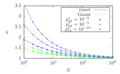
Figure 2: $N$-scaling coefficient $w$ defined in Eq. (40) as a function of $N$, for false-dismissal probability $p_{\mathrm{fD}}^{*}=0.1$, and different false-alarm probabilities $p_{\mathrm{fA}}^{*}\in[10^{-10},10^{-5},10^{-2}]$. Solid lines show the scaling obtained from the exact solution Eq. (27), while dashed lines refer to the Gauss approximation of Eq. (36). The WSG approximation corresponds to $w=1$.

We see that the exact $N$-scaling $w$ increasingly deviates from the WSG approximation ($w=1$) at lower false-alarm probabilities and at smaller $N$. The Gauss approximation tends to agree better with the exact scaling at larger $N$ (as expected), and at higher false-alarm probabilities.

Using the power-law approximation of Eq. (40), we can now express the threshold signal strength of Eq. (29) as

$$L_{0}(N,T,\widetilde{m},\widehat{m}) \equiv\frac{r_{0}\,S_{\mathrm{n}}}{2N_{\mathrm{det}}}\,h_{\mathrm{th}}^{-2}$$

$$=\left[1-\xi(\widetilde{m}+\widehat{m})\right]\,T\,N^{-1/(2w)}\,,$$ (42)

which defines the objective function $L_{0}$ that we want to maximize as a function of the StackSlide parameters.

We see that, without further constraints the optimal solution would simply be $m\rightarrow 0$, $N\rightarrow 1$ and $T\rightarrow T_{\mathrm{max}}$, i.e. a fully coherent search over all the available data $T_{\mathrm{max}}$ with an infinitely fine template bank. This would obviously require infinite computing power, and we therefore need to extend the optimization problem by a computing-cost constraint.

III.4 Template counting

For both the coarse and the fine grid, the respective number of templates $\{\widetilde{\mathcal{N}},\,\widehat{\mathcal{N}}\}$ covering the parameter space $\mathbb{P}$ is given Prix (2007b); Messenger et al. (2009) by the general expression

$$\mathcal{N}=\theta_{n}\,m^{-n/2}\,\mathcal{V}_{n}\,,\quad\mbox{with}\quad\mathcal{V}_{n}\equiv\int_{\mathbb{T}_{n}}\sqrt{\det g}\,d^{n}\lambda\,,$$ (43)

where $m$ is the maximal-mismatch parameter, $\det g$ is the determinant of the corresponding parameter-space metric $g_{ij}$, and $\mathcal{V}_{n}$ denotes the metric volume of the $n$-dimensional space $\mathbb{T}_{n}\subseteq\mathbb{P}$ spanned by the template-bank. The normalized thickness $\theta_{n}$ depends on the geometric structure of the covering, for example $\theta_{\mathbb{Z}_{n}}=n^{n/2}\,2^{-n}$ for a hyper-cubic lattice $\mathbb{Z}_{n}$.

An important subtlety in Eq. (43) is the dimensionality $n$ of the template-bank space $\mathbb{T}_{n}$, which can be smaller than the dimensionality of the parameter space $\mathbb{P}$, as previously discussed in Brady and Creighton (2000); Cutler et al. (2005). The template-bank dimensionality $n$ is generally a (piece-wise constant) function of the StackSlide parameters $\{N,\Delta T,m\}$, which determine the metric resolution. The extent of $\mathbb{P}$ along certain directions can be “thin” compared to the metric resolution and would require only a single template along this direction, effectively not contributing to the template-bank dimensionality. For different StackSlide parameters, however, the resolution might be sufficient to require more than one template along this direction, adding to the template-bank dimensionality $n$.

Following Brady et al. (1998); Brady and Creighton (2000); Cutler et al. (2005), the correct dimensionality for given StackSlide parameters can be determined by the condition that $n$ should maximize the number of templates $\mathcal{N}_{n}$ computed via Eq. (43), i.e.

$$\widetilde{\mathcal{N}}_{{\widetilde{n}}}=\max_{n}\widetilde{\mathcal{N}}_{n}\,,\quad\mbox{and}\quad\widehat{\mathcal{N}}_{{\widehat{n}}}=\max_{n}\widehat{\mathcal{N}}_{n}\,.$$ (44)

This can be understood as follows: if $\mathcal{N}$ decreases when adding a template-bank dimension, then the corresponding parameter-space extent is thinner than the metric resolution and therefore adds “fractional” templates. On the other hand, if $\mathcal{N}$ decreases by removing a dimension, then its extent is thicker than the metric resolution and requires more than one template to cover it.

An interesting alternative formulation can be obtained by expressing Eq. (44) as the condition $\mathcal{N}_{n}/\mathcal{N}_{n-1}>1$ for including an additional dimension $n$. For constant metrics and simple parameter-space shapes, i.e. $\mathcal{V}_{n}=\int\sqrt{g}\,d^{n}\lambda=\sqrt{g}\,\Delta\lambda_{1}\times\Delta\lambda_{2}\ldots\times\Delta\lambda_{n}$, this can be shown to be equivalent to

$$\frac{\theta_{n}}{\theta_{n-1}}\,\frac{\Delta\lambda_{n}}{d\lambda_{n}}>1\,,$$ (45)

where $d\lambda_{n}\equiv\sqrt{m\,g^{nn}}$ is the metric template extent along dimension $n$, in terms of the diagonal element $g^{nn}$ of the inverse metric $g^{ij}$. This shows that Eq. (44) boils down to (apart from the lattice-thickness ratio) the requirement that the parameter-space extent $\Delta\lambda_{n}$ along a given dimension $n$ must exceed the corresponding metric template resolution $d\lambda_{n}$.

The coherent (coarse-grid) metric volume $\widetilde{\mathcal{V}}_{\widetilde{n}}$ is typically a steep function of the coherence time $\Delta T$, and can often be well approximated (over some range of $\Delta T$) by a power law, namely $\widetilde{\mathcal{V}}_{\widetilde{n}}(\Delta T)\propto\Delta T^{\widetilde{q}}$. We can therefore write Eq. (43) for $\widetilde{\mathcal{N}}$ in the power-law form

$$\widetilde{\mathcal{N}}_{\widetilde{n}}(\widetilde{m},\Delta T)=\widetilde{k}\,\widetilde{m}^{-{\widetilde{n}}/2}\,\Delta T^{\widetilde{q}}\,,$$ (46)

where $\widetilde{k}=\theta_{\widetilde{n}}\widetilde{\mathcal{V}}_{\widetilde{n}}(\Delta T_{0})\,\Delta T_{0}^{-\widetilde{q}}$ for some choice of segment length $\Delta T_{0}$.

The semi-coherent (fine-grid) metric volume $\widehat{\mathcal{V}}_{\widehat{n}}$ generally depends on both $\Delta T$ and $N$ and can typically Brady and Creighton (2000); Pletsch (2010); Messenger (2011) be factored in the form

$$\widehat{\mathcal{V}}_{\widehat{n}}(N,\Delta T)=\gamma_{\widehat{n}}(N)\,\widetilde{\mathcal{V}}_{\widehat{n}}(\Delta T)\,,$$ (47)

in terms of the refinement factor $\gamma_{\widehat{n}}(N)\geq 1$ and the coherent-metric volume $\widetilde{\mathcal{V}}_{\widehat{n}}(\Delta T)$ of the fine-grid template space. Typically $\gamma(N)$ can be well approximated (over some range of $N$) by a power law, namely $\gamma(N)\propto N^{\widehat{p}}$. We can therefore write Eq. (43) for $\widehat{\mathcal{N}}$ in the power-law form

$$\widehat{\mathcal{N}}_{\widehat{n}}(\widehat{m},\Delta T,N)=\widehat{k}\,\widehat{m}^{-{\widehat{n}}/2}\,\Delta T^{\widehat{q}}\,N^{\widehat{p}}\,,$$ (48)

where $\widehat{k}=\theta_{\widehat{n}}\widehat{\mathcal{V}}_{\widehat{n}}(\Delta T_{0},N_{0})\,\Delta T_{0}^{-\widehat{q}}N_{0}^{-\widehat{p}}$ for some choice of parameters $\{\Delta T_{0},N_{0}\}$.

III.5 Computing-cost model

The total computing cost $C_{\mathrm{tot}}$ of the interpolating StackSlide statistic has two main contributions, namely

$$C_{\mathrm{tot}}(\widetilde{m},\widehat{m},N,\Delta T)=\widetilde{C}+\widehat{C}\,,$$ (49)

where $\widetilde{C}(\widetilde{m},N,\Delta T)$ is the computing cost of the $\mathcal{F}$-statistic over the coarse grid of $\widetilde{\mathcal{N}}_{\widetilde{n}}$ templates for each of the $N$ segments, and $\widehat{C}(\widehat{m},N,\Delta T)$ is the cost of incoherently summing these $\mathcal{F}$-values across all segments on a fine grid of $\widehat{\mathcal{N}}_{\widehat{n}}$ templates. Note that we neglect all other costs such as data-IO etc, which for any computationally limited search will typically be much smaller than $C_{\mathrm{tot}}$.

III.5.1 Computing cost $\widetilde{C}$ of the coherent step

The computing cost of the coherent step is

$$\widetilde{C}(\widetilde{m},N,\Delta T)=N\,\widetilde{\mathcal{N}}_{\widetilde{n}}(\widetilde{m},\Delta T)\,N_{\mathrm{det}}\,\widetilde{c}_{1}(\Delta T)\,,$$ (50)

where $\widetilde{c}_{1}(\Delta T)$ is the $\mathcal{F}$-statistic computing cost of a single template for a single segment and a single detector. Here we used the fact that to first order Prix (2007a) the number of detectors has no effect on the number of templates $\widetilde{\mathcal{N}}$.

As discussed previously in Cutler et al. (2005), there are two fundamentally different implementations of the $\mathcal{F}$-statistic calculation currently in use: a direct SFT-method Williams and Schutz (1999), and a (generally far more efficient) FFT-method based on barycentric resampling Jaranowski et al. (1998); Patel et al. (2010).

1. The SFT-method consists in interpolating frequency bins of short Fourier transforms (“SFTs”) of length $T_{\mathrm{SFT}}$, using approximations described in Williams and Schutz (1999); Prix (2010). The resulting per-template cost $\widetilde{c}_{1}(\Delta T)$ is directly proportional to the segment length $\Delta T$:

   $$\widetilde{c}_{1}^{\mathrm{SFT}}(\Delta T)=\widetilde{c}_{0}^{\mathrm{SFT}}\,\frac{\Delta T}{T_{\mathrm{SFT}}}\,,$$ (51)

   where $\widetilde{c}_{0}^{\mathrm{SFT}}$ is an implementation- and hardware-dependent fundamental computing cost.

2. In the FFT-method the cost of searching a frequency band $\Delta f$ using an (up-sampled by $u$) FFT frequency-resolution of $u/\Delta T$ is proportional to $\mathcal{N}_{f}\,\log 2\mathcal{N}_{f}$, where $\mathcal{N}_{f}=u\Delta f\,\Delta T$ is the number of frequency bins. We can therefore express the per-template $\mathcal{F}$-statistic cost $\widetilde{c}_{1}(\Delta T)$ as

   $$\widetilde{c}_{1}^{\mathrm{FFT}}(\Delta T)=\widetilde{c}_{0}^{\mathrm{FFT}}\,\log(2u\Delta f\Delta T)\,,$$ (52)

   where $\widetilde{c}_{0}^{\mathrm{FFT}}$ is an implementation- and hardware-dependent fundamental computing cost.

Using the power-law model of Eq. (46) for $\widetilde{\mathcal{N}}$, we can write the coherent computing cost in the form

$$\widetilde{C}(\widetilde{m},N,\Delta T)={\widetilde{\kappa}}\,\widetilde{m}^{-{\widetilde{n}}/2}\,N^{\widetilde{\eta}}\,\Delta T^{{\widetilde{\delta}}}\,,$$ (53)

where

$${\widetilde{\eta}}=1,\quad{\widetilde{\delta}}=\widetilde{q}+\Delta{\widetilde{\delta}}\,,$$ (54)

and where $\Delta{\widetilde{\delta}}$ is either

$$\Delta{\widetilde{\delta}}=\begin{cases}\Delta{\widetilde{\delta}}_{\mathrm{SFT}}\equiv 1\,,\\ \Delta{\widetilde{\delta}}_{\mathrm{FFT}}\equiv\left[\log(2u\Delta f\Delta T_{0})\right]^{-1}\,,\\ \end{cases}$$ (55)

depending on whether the $\mathcal{F}$-statistic is computed using the SFT- or FFT-method, respectively. The expression for $\Delta{\widetilde{\delta}}_{\mathrm{FFT}}$ can be obtained via Eq. (62) and depends (albeit weakly) on the reference segment length $\Delta T_{0}$. The corresponding proportionality factors ${\widetilde{\kappa}}$ are found as

$$\begin{split}{\widetilde{\kappa}}_{\mathrm{SFT}}&=\theta_{\widetilde{n}}\,N_{\mathrm{det}}\,\frac{\widetilde{c}_{0}^{\mathrm{SFT}}}{T_{\mathrm{SFT}}}\,\frac{\widetilde{\mathcal{V}}_{\widetilde{n}}(\Delta T_{0})}{\Delta T_{0}^{\widetilde{q}}}\,,\\ {\widetilde{\kappa}}_{\mathrm{FFT}}&=\theta_{\widetilde{n}}\,N_{\mathrm{det}}\,\frac{\widetilde{c}_{0}^{\mathrm{FFT}}}{\Delta{\widetilde{\delta}}_{\mathrm{FFT}}}\,\frac{\widetilde{\mathcal{V}}_{\widetilde{n}}(\Delta T_{0})}{\Delta T_{0}^{{\widetilde{\delta}}}}\,.\end{split}$$ (56)

III.5.2 Computing cost $\widehat{C}$ of the incoherent step

The computing cost of the StackSlide step is

$$\widehat{C}(\widehat{m},N,\Delta T)=N\,\widehat{\mathcal{N}}_{\widehat{n}}(\widehat{m},\Delta T,N)\,\widehat{c}_{0}\,,$$ (57)

where $\widehat{c}_{0}$ is the implementation- and hardware-dependent fundamental cost of adding one value of $2\mathcal{F}_{k}$ for one fine-grid point $\widehat{\lambda}$ in Eq. (2), including the cost of mapping the fine-grid point to its closest coarse-grid template $\widetilde{\lambda}_{k}(\widehat{\lambda})$. The incoherent step operates on coherent multi-detector $\mathcal{F}$-statistic values, and therefore does not depend on the number of detectors $N_{\mathrm{det}}$.

Using the power-law model of Eq. (48) for $\widehat{\mathcal{N}}$, we can write the incoherent computing cost as

$$\widehat{C}(\widehat{m},N,\Delta T)=\widehat{\kappa}\,\widehat{m}^{-{\widehat{n}}/2}\,N^{\widehat{\eta}}\,\Delta T^{\widehat{\delta}}\,,$$ (58)

where

$${\widehat{\eta}}=\widehat{p}+1\,,\quad{\widehat{\delta}}=\widehat{q}\,,$$ (59)

and the proportionality factor

$${\widehat{\kappa}}=\theta_{\widehat{n}}\,\widehat{c}_{0}\,\,\frac{\widehat{\mathcal{V}}_{\widehat{n}}(N_{0},\Delta T_{0})}{N_{0}^{\widehat{p}}\,\Delta T_{0}^{\widehat{q}}}\,,$$ (60)

for given reference values $\{N_{0},\Delta T_{0}\}$.

III.5.3 General power-law computing-cost model

Combining Eqs. (53) and (58) we arrive at the following power-law model for the total computing cost, defined in Eq. (49), namely

$$C_{\mathrm{tot}}={\widetilde{\kappa}}\,\widetilde{m}^{-{\widetilde{n}}/2}\,N^{\widetilde{\eta}}\,\Delta T^{\widetilde{\delta}}+{\widehat{\kappa}}\,\widehat{m}^{-{\widehat{n}}/2}\,N^{\widehat{\eta}}\,\Delta T^{\widehat{\delta}}\,.$$ (61)

If a given computing-cost function does not follow this model, we can always produce a local fit to Eq. (61), which should be valid over some range of parameters $\{\Delta T,N\}$, namely

$$\delta\equiv\left.\frac{\partial\log C}{\partial\log\Delta T}\right.\,,\quad\eta\equiv\left.\frac{\partial\log C}{\partial\log N}\right.\,,$$ (62)

$$\kappa\equiv\frac{C(m_{0},N_{0},\Delta T_{0})}{m_{0}^{-n/2}\,N_{0}^{\eta}\,\Delta T_{0}^{\delta}}\,,$$ (63)

for reference values $\{m_{0},N_{0},\Delta T_{0}\}$. Note that $\delta$ generally depends only on $\Delta T_{0}$, while $\eta$ depends only on $N_{0}$, due to the way these dependencies typically factor (cf. Sec. III.5). The mismatch dependency $\propto m^{-n/2}$ is exact according to Eq. (43), but a given computing-cost function might still deviate from this behaviour (e.g. the BC/CGK computing-cost function discussed in Sec. V.3). In this case one can extend the power-law fit by extracting the “mismatch-dimension” $n$ via

$$n\equiv-2\,\left.\frac{\partial\log C}{\partial\log m}\right.\,.$$ (64)

It will be more convenient in the following to work in terms of $\{N,T\}$ instead of $\{N,\Delta T\}$, where $T=N\,\Delta T$ is the total time span of data used. Changing variables, we obtain the computing-cost model in the form

$$C_{\mathrm{tot}}={\widetilde{\kappa}}\,\widetilde{m}^{-{\widetilde{n}}/2}\,N^{-{\widetilde{\varepsilon}}}\,T^{\widetilde{\delta}}+{\widehat{\kappa}}\,\widehat{m}^{-{\widehat{n}}/2}\,N^{-{\widehat{\varepsilon}}}\,T^{\widehat{\delta}}\,,$$ (65)

where we defined

$$\varepsilon\equiv\delta-\eta\,,$$ (66)

generally satisfying $\varepsilon>0$ for all realistic cases considered here. Note that $m$ and $N$ are dimensionless, therefore the respective units of $[C/\kappa]$ are $[T^{\delta}]$.

Symbol	Description	Relations	Refs
$N$	Number of segments		Sec. III, Eq. (1)
$\Delta T$	Segment duration		Sec. III
$T$	Total observation time	$T=N\,\Delta T$	Sec. III
$\widetilde{Q}$	a quantity $Q$ referring to the coherent step		Sec. III
$\widehat{Q}$	a quantity $Q$ referring to the incoherent step		Sec. III
$n$	number of template-bank dimensions		Eq. (44)
$m$	maximal template-bank mismatch parameter		Eqs. (8), (15)
$\xi$	average mismatch factor $\in[0,1]$	$\left\langle\mu\right\rangle=\xi\,m$	Eq. (23)
$w$	$L_{0}$ sensitivity scaling with $N$	$\left.L_{0}\right|_{m,T}\propto N^{-1/(2w)}$	Eq. (40)
$\varpi$	Lagrange multiplier for computing-cost constraint	$L=L_{0}+\varpi(C_{\mathrm{tot}}-C_{0})$	Eq. (67)
$\kappa$	computing-cost prefactor		Eqs. (53),(58)
$\delta$	computing-cost $T$- or $\Delta T$- exponent at fixed $N$	$\left.C\right|_{N}\propto\Delta T^{\delta}\propto T^{\delta}$	Eqs. (53),(58)
$\eta$	computing-cost $N$-exponent at fixed $\Delta T$	$\left.C\right|_{\Delta T}\propto N^{\eta}$	Eqs. (53),(58)
$-\varepsilon$	computing-cost $N$-exponent at fixed $T$	$\left.C\right|_{T}\propto N^{-\varepsilon}$	Eq. (65)

Table 1: Overview of symbols and notation used in the formulation of the optimization problem.

IV Maximizing sensitivity at fixed computing cost

We want to maximize the objective function $L_{0}\propto h_{\mathrm{th}}^{-2}$ defined in Eq. (42) under the constraint of fixed computing cost, $C_{\mathrm{tot}}=C_{0}$. We therefore need to find the stationary points of the Lagrange function

$$L(N,T,\widetilde{m},\widehat{m},\varpi)=L_{0}+\varpi\,[\widetilde{C}+\widehat{C}-C_{0}]\,,$$ (67)

where stationarity with respect to the Lagrange multiplier, i.e. $\partial_{\varpi}L=0$, returns the computing-cost constraint $\widetilde{C}+\widehat{C}=C_{0}$.

Table 1 provides a “dictionary” summarizing the notation used here and in the previous section to formulate the optimization problem.

Before embarking on the full optimization problem, it is instructive to consider two special cases, namely (i) a fully coherent search, and (ii) searches where the computing cost is dominated by one contribution, either coherent $\widetilde{C}$ or incoherent $\widehat{C}$.

IV.1 Special case (i): Fully coherent search

The fully coherent search is a special case of Eq. (67) with the additional constraint $N=1$, and therefore  $\Delta T=T$, $\widehat{m}=0$, and $\widehat{C}=0$. This leaves us with the reduced Lagrangian

$$L(T,\widetilde{m},\varpi)=(1-\xi\widetilde{m})\,T+\varpi\,[{\widetilde{\kappa}}\,\widetilde{m}^{-{\widetilde{n}}/2}\,T^{\widetilde{\delta}}-C_{0}]\,.$$ (68)

Requiring stationarity with respect to $\{T,\widetilde{m},\varpi\}$ results in the optimal StackSlide parameters

$$\xi\,{\widetilde{m}}_{\mathrm{opt}} =\left(1+\frac{2{\widetilde{\delta}}}{{\widetilde{n}}}\right)^{-1}\,,$$ (69)

$${T}_{\mathrm{opt}} =\left(\frac{C_{0}}{{\widetilde{\kappa}}}\right)^{1/{\widetilde{\delta}}}\,{\widetilde{m}}_{\mathrm{opt}}^{{\widetilde{n}}/(2{\widetilde{\delta}})}\,.$$ (70)

Interestingly the optimal mismatch ${\widetilde{m}}_{\mathrm{opt}}$ is independent of both the computing-cost constraint $C_{0}$ and the observation time $T$. The scaling of the resulting threshold signal strength $h_{\mathrm{th}}$ with computing cost $C_{0}$ is therefore

$$h_{\mathrm{th}}^{-1}\propto C_{0}^{1/(2{\widetilde{\delta}})}\,.$$ (71)

In practical applications we often find ${\widetilde{\delta}}\approx 3-7$, and so ${T}_{\mathrm{opt}}$ and $h_{\mathrm{th}}^{-1}$ will increase very slowly with increasing computing cost $C_{0}$. This indicates that a brute-force approach of throwing more computing power at a fully coherent search will typically yield meagre returns in sensitivity.

IV.2 Special case (ii): Computing cost dominated by one contribution

If either the coherent $\widetilde{C}$ or incoherent $\widehat{C}$ contribution dominates the total computing cost (65), we can write

$$C_{\mathrm{tot}}\approx\kappa\,m^{-n/2}\,N^{-\varepsilon}\,T^{\delta}\,,$$ (72)

where all StackSlide parameters now refer to dominant contribution only.

We assume that the negligible computing-cost contribution implies that we can also neglect the corresponding mismatch: if the respective step is cheap, one can easily increase sensitivity by reducing the corresponding mismatch until it is negligible, i.e. we assume $\left\langle\mu_{\mathrm{sc}}\right\rangle\approx\xi\,m$. This qualitative argument will be confirmed by the general solution in the next section. We can therefore write the objective function Eq. (42) as

$$L_{0}(N,T,{m})\approx(1-\xi\,m)\,N^{-1/(2w)}\,T\,.$$ (73)

Using Eq. (72) we can obtain

$$N(C_{0},m,T) =(C_{0}/\kappa)^{-1/\varepsilon}\,m^{-n/(2\varepsilon)}\,T^{\delta/\varepsilon}\,,$$ (74)

$$\Delta T(C_{0},m,T) =(C_{0}/\kappa)^{1/\varepsilon}\,m^{n/(2\varepsilon)}\,T^{-\eta/\varepsilon}\,,$$ (75)

which shows that increasing $T$ at fixed $C_{0}$ results in more and shorter segments, while increasing $C_{0}$ at fixed $T$ results in fewer and longer segments (assuming $\varepsilon>0$). Substituting this into Eq. (73) yields the threshold signal strength

$$h_{\mathrm{th}}^{-2}\propto(C_{0}/\kappa)^{1/(2w\varepsilon)}\,\left[(1-\xi m)\,m^{n/(4w\varepsilon)}\right]\,\,T^{\,a/{(2w\varepsilon)}}\,,$$ (76)

where we introduced the parameter

$$a\equiv 2w\varepsilon-\delta\,,$$ (77)

which will be of critical importance in determining the character of the optimal solution.

The objective function $L_{0}\propto h_{\mathrm{th}}^{-2}$ can be easily maximized over mismatch $m$, resulting in

$$\xi\,{m}^{(0)}_{\mathrm{opt}}=\left[1+\frac{4w\varepsilon}{n}\right]^{-1}\,,$$ (78)

which is independent of both $C_{0}$ and $T$. This solution differs from Eq. (69) of the fully coherent case, even when the coherent cost dominates (where ${\widetilde{\varepsilon}}={\widetilde{\delta}}-1$).

We see in Eq. (76) that there is no extremum of $h_{\mathrm{th}}$ (at least in regions of approximately constant power-law exponents). Given that $w\geq 1$ and generally $\varepsilon>0$, we can distinguish two different regimes depending on the sign of critical scaling exponent $a$ defined in Eq. (77):

$a>0$:

sensitivity improves (i.e. $h_{\mathrm{th}}^{-1}$ increases) with increasing $T$ (at fixed $C_{0}$). Therefore sensitivity is only limited by the total amount of data $T_{\mathrm{max}}$ available.

$a<0$:

sensitivity improves with decreasing $T$, so one should use less data (until the assumptions change).

In practice these extreme conclusions will be modified, as the power-law exponents will vary (slowly) as functions of $N$ and $T$, and the assumption of a dominating computing-cost contribution might also no longer be satisfied. The marginal case $a=0$ marks a possible sensitivity maximum, namely if increasing $T$ results in $a<0$ and decreasing $T$ leads to $a>0$.

We can obtain a useful qualitative picture of the full optimization problem by considering the two extreme cases of dominating computing contribution $\widetilde{C}$ or $\widehat{C}$:

• if $\widetilde{C}\gg\widehat{C}$: we always have $\widetilde{a}>0$ (for all cases of interest ${\widetilde{\eta}}=1$, ${\widetilde{\delta}}>2$ and $w\geq 1$). Therefore sensitivity improves with increasing $T$. As seen in Sec. IV.3.3 this shifts computing cost to the incoherent contribution. Eventually one either uses all the data $T_{\mathrm{max}}$ or the coherent cost no longer dominates.

• if $\widehat{C}\gg\widetilde{C}$: the incoherent parameter $\widehat{a}$ can have any sign. If $\widehat{a}>0$ one would increase $T$ until all the data $T_{\mathrm{max}}$ is used (or we reach $\widehat{a}=0$). If $\widehat{a}<0$ one would decrease $T$ until the incoherent cost no longer dominates.

These limiting cases show that the type of optimal solution will be determined solely by the incoherent critical exponent $\widehat{a}=2w{\widehat{\varepsilon}}-{\widehat{\delta}}$, namely

$${T}^{(0)}_{\mathrm{opt}}=\begin{cases}\text{finite}&\text{if $\widehat{a}\leq 0$}\,,\\ \infty&\text{otherwise}\,,\end{cases}$$ (79)

which we refer to as the bounded and the unbounded regime, respectively.

IV.3 General optimality conditions

We now return to the full optimization problem of Eq. (67), namely

$$L=L_{0}+\varpi\,[\widetilde{C}+\widehat{C}-C_{0}]\,,$$ (80)

where

$$L_{0} =\left[1-\xi(\widetilde{m}+\widehat{m})\right]\,{T}\,N^{-1/(2w)}\,,$$ (81)

$$\widetilde{C} ={\widetilde{\kappa}}\,\widetilde{m}^{-{\widetilde{n}}/2}\,N^{-{\widetilde{\varepsilon}}}\,T^{\widetilde{\delta}}\,,$$ (82)

$$\widehat{C} ={\widehat{\kappa}}\,\widehat{m}^{-{\widehat{n}}/2}\,N^{-{\widehat{\varepsilon}}}\,T^{\widehat{\delta}}\,.$$ (83)

It will be useful introduce the computing-cost ratio

$$\varkappa\equiv{\widetilde{C}}/{\widehat{C}}\,,$$ (84)

and express the respective contributions as

$$\widetilde{C}=\frac{C_{0}}{1+\varkappa^{-1}}\,,\quad\widehat{C}=\frac{C_{0}}{1+\varkappa}\,.$$ (85)

Using Eqs. (82), (83) to solve for $T$ and $N$, respectively, we obtain

$$N^{D} =\frac{(C_{0}/{\widehat{\kappa}})^{{\widetilde{\delta}}}}{(C_{0}/{\widetilde{\kappa}})^{{\widehat{\delta}}}}\,\frac{\left[\widetilde{m}^{-{\widetilde{n}}/2}\,(1+\varkappa^{-1})\right]^{\widehat{\delta}}}{\left[\widehat{m}^{-{\widehat{n}}/2}\,(1+\varkappa)\right]^{\widetilde{\delta}}}\,,$$ (86)

$$T^{D} =\frac{(C_{0}/{\widehat{\kappa}})^{{\widetilde{\varepsilon}}}}{(C_{0}/{\widetilde{\kappa}})^{\widehat{\varepsilon}}}\,\frac{\left[\widetilde{m}^{-{\widetilde{n}}/2}\,(1+\varkappa^{-1})\right]^{\widehat{\varepsilon}}}{\left[\widehat{m}^{-{\widehat{n}}/2}\,(1+\varkappa)\right]^{\widetilde{\varepsilon}}}\,,$$ (87)

where $D$ is the determinant of the matrix $[{\widetilde{\delta}},{\widetilde{\eta}};{\widehat{\delta}},{\widehat{\eta}}]$, which for all cases of practical interest seems to be positive definite, namely

$$D\equiv{\widetilde{\delta}}{\widehat{\eta}}-{\widehat{\delta}}\,{\widetilde{\eta}}>0\,.$$ (88)

The segment length $\Delta T=T/N$ can similarly be obtained as

$$\Delta T^{D}=\frac{(C_{0}/{\widetilde{\kappa}})^{{\widehat{\eta}}}}{(C_{0}/{\widehat{\kappa}})^{{\widetilde{\eta}}}}\,\frac{\left[\widehat{m}^{-{\widehat{n}}/2}\,(1+\varkappa)\right]^{\widetilde{\eta}}}{\left[\widetilde{m}^{-{\widetilde{n}}/2}\,(1+\varkappa^{-1})\right]^{\widehat{\eta}}}\,.$$ (89)

IV.3.1 Stationarity with respect to mismatches $\{\widetilde{m},\widehat{m}\}$

Requiring stationarity with respect to the mismatches, i.e. $\partial_{\widetilde{m}}L=\partial_{\widehat{m}}L=0$, yields

$$\begin{split}\varpi\widetilde{C}&=-2\xi\,\frac{{\widetilde{m}}_{\mathrm{opt}}}{{\widetilde{n}}}\,{T}N^{-1/(2w)}\,,\\ \varpi\widehat{C}&=-2\xi\,\frac{{\widehat{m}}_{\mathrm{opt}}}{{\widehat{n}}}\,{T}N^{-1/(2w)}\,,\end{split}$$ (90)

which results in the remarkable relation

$$\frac{{\widetilde{m}}_{\mathrm{opt}}/{\widetilde{n}}}{{\widehat{m}}_{\mathrm{opt}}/{\widehat{n}}}=\varkappa\,.$$ (91)

The ratio of optimal mismatch per dimension is simply given by the computing-cost ratio $\varkappa$. This result confirms an assumption made in Sec. IV.2 about the optimal solution, namely that a negligible computing-cost contribution also implies that one can neglect the corresponding mismatch.

IV.3.2 Stationarity with respect to number of segments $N$

Requiring stationarity with respect to $N$ (treated as continuous), i.e. $\partial_{N}L=0$ yields

$$L_{0}+2w\,\varpi\left[{\widetilde{\varepsilon}}\,\widetilde{C}+{\widehat{\varepsilon}}\,\widehat{C}\right]=0\,,$$ (92)

and substituting Eqs. (90) and (81), we obtain

$$\frac{{\widetilde{m}}_{\mathrm{opt}}}{{\widetilde{m}}^{(0)}_{\mathrm{opt}}}+\frac{{\widehat{m}}_{\mathrm{opt}}}{{\widehat{m}}^{(0)}_{\mathrm{opt}}}=1\,,$$ (93)

where we used the asymptotic optimal mismatches ${m}^{(0)}_{\mathrm{opt}}$ defined in Eq. (78) for the two limiting cases of dominating coherent or incoherent computing-cost, respectively. Equation (93) can be interpreted as defining a two-dimensional ellipse in $\sqrt{m}$ with semi-major axes $\sqrt{{m}^{(0)}_{\mathrm{opt}}}$. Combining this with Eq. (91) we obtain the optimal mismatches

$$\begin{split}\frac{{\widetilde{n}}}{{\widetilde{m}}_{\mathrm{opt}}}&=\frac{{\widetilde{n}}}{{\widetilde{m}}^{(0)}_{\mathrm{opt}}}+\frac{{\widehat{n}}}{{\widehat{m}}^{(0)}_{\mathrm{opt}}}\,\varkappa^{-1}\,,\\ \frac{{\widehat{n}}}{{\widehat{m}}_{\mathrm{opt}}}&=\frac{{\widehat{n}}}{{\widehat{m}}^{(0)}_{\mathrm{opt}}}+\frac{{\widetilde{n}}}{{\widetilde{m}}^{(0)}_{\mathrm{opt}}}\,\varkappa\,,\end{split}$$ (94)

which reduces to the limiting cases of Eq. (78) when either computing cost dominates, i.e. when $\varkappa\ll 1$ or $\varkappa\gg 1$. We can express the optimal mismatch prefactor in Eq. (81) as

$${\left[1-\xi(\widetilde{m}+\widehat{m})\right]}_{\mathrm{opt}}=\left[1+\frac{1}{4w}\frac{\widetilde{n}\varkappa+\widehat{n}}{\widetilde{\varepsilon}\varkappa+\widehat{\varepsilon}}\right]^{-1}\,.$$ (95)

The optimal mismatches Eq. (94) only depend on the computing-cost ratio $\varkappa$. Substituting into Eq. (87) we therefore obtain a relation of the form $T_{0}=T(C_{0},{\varkappa}_{\mathrm{opt}})$ for given observation time $T_{0}$, which can (numerically) be solved for ${\varkappa}_{\mathrm{opt}}=\varkappa(C_{0},T_{0})$. Similarly, one could specify $N_{0}$ and solve Eq. (86) for ${\varkappa}_{\mathrm{opt}}=\varkappa(C_{0},N_{0})$. In either case the optimal mismatches are obtained from Eq. (94) and the optimal number and length of segments from Eqs. (86) and (87), fully closing the optimal solution at fixed $T$.

IV.3.3 Monotonicity relations with $T$

It is interesting to consider the behaviour of the optimal “fixed-$T$” solution of the previous section as a function of $T$. We see in Eq. (94) that ${\widetilde{m}}_{\mathrm{opt}}$ is monotonically increasing with $\varkappa$, while ${\widehat{m}}_{\mathrm{opt}}$ is decreasing, i.e.

$$\partial_{\varkappa}{\widetilde{m}}_{\mathrm{opt}}>0,\quad\mbox{and}\quad\partial_{\varkappa}{\widehat{m}}_{\mathrm{opt}}<0\,.$$ (96)

We generally assume $D\equiv{\widetilde{\delta}}{\widehat{\eta}}-{\widehat{\delta}}{\widetilde{\eta}}>0$ and $\varepsilon>0$ which implies that the right-hand side of Eq. (87) is monotonically decreasing with $\varkappa$, while the left-hand side is monotonically increasing with $T$. Therefore $\varkappa$ must be montonically decreasing with $T$, i.e.

$$\partial_{T}\varkappa<0\,.$$ (97)

Therefore the optimal solution shifts computing cost from the coherent to the incoherent step with increasing $T$, which had already been used in Sec. IV.2. Combining this with Eq. (96) we find

$$\partial_{T}{\widetilde{m}}_{\mathrm{opt}}<0,\quad\mbox{and}\quad\partial_{T}{\widehat{m}}_{\mathrm{opt}}>0\,,$$ (98)

and using this with Eqs. (86) and (89), we can further deduce

$$\partial_{T}{N}_{\mathrm{opt}}>0\,,\quad\mbox{and}\quad\partial_{T}{\Delta T}_{\mathrm{opt}}<0\,,$$ (99)

namely increasing $T$ results in more segments of shorter duration.

IV.3.4 Stationarity with respect to observation time $T$

Requiring stationarity of $L$ with respect to $T$, i.e. $\partial_{T}L=0$, yields the final condition

$$L_{0}+\varpi\left[{\widetilde{\delta}}\,\widetilde{C}+{\widehat{\delta}}\,\widehat{C}\right]=0\,,$$ (100)

which combined with Eq. (92) results in

$$\widetilde{a}\,\widetilde{C}+\widehat{a}\,\widehat{C}=0\,,$$ (101)

where the critical exponents $a$ are defined in Eq. (77). We generally expect $\widetilde{a}>0$, as discussed in Sec. IV.2, and therefore the stationarity condition can only have a solution if

$$\widehat{a}\equiv{\widehat{\delta}}-2{\widehat{\eta}}+2(w-1)\,{\widehat{\varepsilon}}\,<\,0\,.$$ (102)

This conclusion is consistent with the analysis of Sec. IV.2: $\widehat{a}<0$ characterizes a bounded regime with finite optimal ${T}^{(0)}_{\mathrm{opt}}$, while $\widehat{a}>0$ characterizes an unbounded regime with ${T}^{(0)}_{\mathrm{opt}}\rightarrow\infty$.

If ${T}^{(0)}_{\mathrm{opt}}$ exceeds the available data $T_{\mathrm{max}}$, then we simply apply the fixed-$T$ solution of Sec. IV.3.2. Otherwise Eq. (101) directly yields

$${\varkappa}_{\mathrm{opt}}=-\frac{\widehat{a}}{\widetilde{a}}\,,$$ (103)

closing the optimal solution via Eqs. (94), (86) and (87).

IV.3.5 Monotonicity relations with $C_{0}$

For a bounded optimal solution with ${T}^{(0)}_{\mathrm{opt}}\leq T_{\mathrm{max}}$, we see from Eq. (103) that ${\varkappa}_{\mathrm{opt}}$ and $\{{\widetilde{m}}_{\mathrm{opt}},\,{\widehat{m}}_{\mathrm{opt}}\}$ are independent of the computing-cost constraint $C_{0}$. Inserting Eqs. (86),(87) into Eq. (42), we can therefore read off the scaling

$$h_{\mathrm{th}}^{-1}\propto C_{0}^{(\widetilde{a}-\widehat{a})/(4wD)}\,,$$ (104)

which shows that any “reasonable” search should satisfy

$$\widetilde{a}>\widehat{a}\,,$$ (105)

in order for sensitivity to improve with increasing $C_{0}$ (assuming $D>0$). Furthermore, from Eqs. (86), (87) and (89) we obtain the monotonicity relations:

$$\begin{split}\partial_{C_{0}}{N}_{\mathrm{opt}}&\propto{\widetilde{\delta}}-{\widehat{\delta}}\,,\\ \partial_{C_{0}}{T}_{\mathrm{opt}}&\propto{\widetilde{\varepsilon}}-{\widehat{\varepsilon}}\,,\\ \partial_{C_{0}}{\Delta T}_{\mathrm{opt}}&\propto{\widehat{\eta}}-{\widetilde{\eta}}\,.\end{split}$$ (106)

We expect ${\widehat{\eta}}>{\widetilde{\eta}}=1$, therefore the optimal segment length ${\Delta T}_{\mathrm{opt}}$ will generally increase with $C_{0}$.

The behaviour of the optimal number of segments is less clear-cut: if ${\widetilde{\delta}}<{\widehat{\delta}}$ then ${N}_{\mathrm{opt}}$ decreases with $C_{0}$, which can result in a fully coherent search being optimal, despite ${T}^{(0)}_{\mathrm{opt}}<T_{\mathrm{max}}$. A StackSlide search is therefore not guaranteed to be more sensitive than a fully coherent search at the same computing power, even when computationally limited.

Similarly, ${T}_{\mathrm{opt}}$ can either increase with $C_{0}$ (if ${\widetilde{\varepsilon}}>{\widehat{\varepsilon}}$), or decrease: a more expensive and more sensitive search can be using less data.

V Examples of practical application

In order to illustrate the practical application of this analytical framework and its potential gains in sensitivity we consider a few different examples of CW searches.

V.1 Directed searches for isolated neutron stars

Directed searches target NSs with known sky-position but unknown frequency and frequency derivatives, i.e. $\{f,\dot{f},\ddot{f},\ldots\}$. The approximate phase metric of this parameter space for isolated NSs is known analytically and constant over the parameter space, e.g. see [Eq. (10) in Wette et al. (2008)]. The number of coarse-grid templates scales as

$$\widetilde{\mathcal{N}}\propto\Delta T^{n(n+1)/2}\,,$$ (107)

while the refinement of the semi-coherent metric [Eq. (92) in Pletsch (2010)] scales as

$$\gamma_{n}\propto N^{n(n-1)/2}\,.$$ (108)

The coherent computing-cost exponents Eq. (54) are therefore

$${\widetilde{\delta}}={\widetilde{n}}({\widetilde{n}}+1)/2+\Delta{\widetilde{\delta}}\,,\quad{\widetilde{\eta}}=1\,,$$ (109)

where $\Delta{\widetilde{\delta}}$ depends on the $\mathcal{F}$-statistic implementation as given by Eq. (55). The incoherent computing-cost exponents Eq. (59) are

$${\widehat{\delta}}={\widehat{n}}({\widehat{n}}+1)/2\,,\quad{\widehat{\eta}}=1+{\widehat{n}}({\widehat{n}}-1)/2\,,$$ (110)

which results in ${\widehat{\varepsilon}}={\widehat{n}}-1$.

For ${\widetilde{n}}\geq 2$ the condition $\widetilde{a}={\widetilde{\delta}}-2+2(w-1){\widetilde{\varepsilon}}>0$ holds as expected, while the critical boundedness parameter of Eq. (102) now reads as

$$\widehat{a}=\frac{{\widehat{n}}}{2}(3-{\widehat{n}})-2+2(w-1)({\widehat{n}}-1)\,,$$ (111)

which for the first few values of $n$ evaluates to

$$\begin{split}\widehat{a}_{1}&=-1\,,\\ \widehat{a}_{2}&=-3+2w\,,\\ \widehat{a}_{3}&=-6+4w\,,\\ \widehat{a}_{4}&=-10+6w.\end{split}$$ (112)

In the WSG limit (i.e. $w\rightarrow 1$) this is always $\widehat{a}<0$, and therefore the search falls into the bounded regime. However, in general $w>1$ and therefore directed StackSlide searches can be either bounded or unbounded.

Directed search for Cassiopeia-A

As a concrete example we consider the directed search for the compact object in Cassiopeia-A (CasA). This search has been performed using LIGO S5 data, and the resulting upper limits have been published in Abadie et al. (2010). For the present example we use the search setup as originally proposed in Wette et al. (2008), namely a fully coherent $\mathcal{F}$-statistic search (using the “SFT” method, i.e. $\Delta{\widetilde{\delta}}=1$) using data spanning $T=12\,\mathrm{days}$, with a maximal template-bank mismatch of $\widetilde{m}=0.2$. The setup assumed two detectors with identical noise floor $S_{\mathrm{n}}$ and a $70\%$ duty cycle, which we can formally incorporate as $N_{\mathrm{det}}=2\times 0.7=1.4$ in Eqs. (50) and (29). The parameter space spanned a frequency range of $f\in[100,300]\,\mathrm{Hz}$ and spindown-ranges corresponding to a spindown-age of $\tau=300\,\mathrm{y}$, see Wette et al. (2008). The template-bank dimension for the given StackSlide parameters was determined as ${\widetilde{n}}=3$, resulting in a power-law scaling of ${\widetilde{\delta}}=7$ according to Eq. (109).

In order to compare sensitivity estimates of different search setups, we use nominal (per-template) false-alarm and false-dismissal probabilities of

$$p_{\mathrm{fA}}^{*}=10^{-10},\qquad p_{\mathrm{fD}}^{*}=0.1\,.$$ (113)

We use a rough estimate of $\xi=0.5$ (e.g. see [Fig. 8 in Messenger et al. (2009)]) for the geometric average-mismatch factor of the $A_{3}^{*}$-lattice that was used in this search. Integrating Eqs. (25),(26) and solving for $\rho_{\mathcal{F}}^{*}$ yields $\rho_{\mathcal{F}}^{*}\approx 8.35$. Substituting this into Eq. (29) with $\widehat{m}=0$, $\widetilde{m}=0.2$ yields an estimate for the weakest detectable signal $h_{\mathrm{th}}$ of the original $\mathcal{F}$-statistic search:

$$\left.\frac{h_{\mathrm{th}}}{\sqrt{S_{\mathrm{n}}}}\right|_{\mathrm{ref}}\approx 5.2\times 10^{-3}\,\sqrt{\mathrm{Hz}},$$ (114)

Timing a current StackSlide code using the SFT-method, one can extract approximate timing parameters

$$\widetilde{c}_{0}^{\mathrm{SFT}}=7\times 10^{-8}\,\mathrm{s},\qquad\widehat{c}_{0}=6\times 10^{-9}\,\mathrm{s}\,,$$ (115)

which results in a total computing cost for the original search of $C_{0}\approx 472\,\mathrm{days}$ on a single cluster node. This number is used as the computing-cost constraint $C_{0}$ for this example.

First we consider an optimal coherent search as described in Sec. IV.1, namely using Eq. (69) we find

$$\xi\,{\widetilde{m}}_{\mathrm{opt}}\approx 0.18\quad\Longrightarrow{\widetilde{m}}_{\mathrm{opt}}\approx 0.36\,,$$ (116)

and using Eq. (70) this results in ${T}_{\mathrm{opt}}=13.6\,\mathrm{days}$, which is only about $\sim 13\%$ longer then the original search proposal of Wette et al. (2008). The total improvement in the minimal signal strength $h_{\mathrm{th}}$ is less than $2\%$ compared to Eq. (114), which shows that the original search proposal was remarkably close to an optimal coherent search.

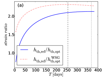
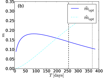
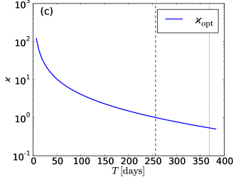
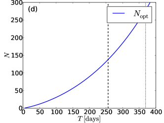
Figure 3: Numerical optimal fixed-$T$ solution for a directed CasA search as a function of $T$. The dashed vertical line indicates the analytical WSG-optimal solution of Eq. (118), while the dotted vertical line corresponds to the exact optimal solution. Panel (a) shows the weakest detectable signal strength compared to the reference value $h_{\mathrm{th},\mathrm{ref}}$ of Eq. (114), for the exact $h_{\mathrm{th}}$ and for the WSG-approximated $h_{\mathrm{th}}^{\mathrm{WSG}}$ (using $w=1$). (b) shows the optimal mismatch parameters ${\widetilde{m}}_{\mathrm{opt}}(T)$ and ${\widehat{m}}_{\mathrm{opt}}(T)$, (c) shows the optimal computing-cost ratio ${\varkappa}_{\mathrm{opt}}(T)$ and (d) the optimal number of segments ${N}_{\mathrm{opt}}(T)$ (treated as continuous).

Next we consider a StackSlide search over the same parameter space using the same computing cost $C_{0}$. Assuming the optimal solution will have segment lengths in the range $1\;\mathrm{days}\lesssim\Delta T\lesssim 7\;\mathrm{days}$, and a total span of $T\lesssim 365\,\mathrm{days}$, the parameter-space dimensions would be ${\widetilde{n}}=2$, ${\widehat{n}}=3$ (see Wette et al. (2008)). This results in power-law exponents ${\widetilde{\delta}}=4$, ${\widehat{\delta}}=6\,,\;{\widehat{\eta}}=4$, and therefore ${\widetilde{\varepsilon}}=3$, ${\widehat{\varepsilon}}=2$, and $\widetilde{a}=2+6(w-1)$, $\widehat{a}=-2+4(w-1)$. In order to simplify the example we use the WSG approximation, i.e. $w=1$, which implies that the search would be bounded ($\widehat{a}<0$). We can therefore use Eq. (103) to obtain the optimal computing-cost ratio as

$${\varkappa}_{\mathrm{opt}}=1\,.$$ (117)

Note that when $w>1.25$ we would have $\widehat{a}>0$ and therefore this search would become unbounded. From Eq. (78) we obtain ${\widetilde{m}}^{(0)}_{\mathrm{opt}}\approx 0.29$, ${\widehat{m}}^{(0)}_{\mathrm{opt}}\approx 0.55$, and using Eq. (94) we find the respective optimal mismatches as

$${\widetilde{m}}_{\mathrm{opt}}\approx 0.16\,,\quad{\widehat{m}}_{\mathrm{opt}}\approx 0.24\,.$$ (118)

Using Eq. (63) we can extract the computing-cost coefficients ${\widetilde{\kappa}}\approx 3.14\times 10^{-17}$ and ${\widehat{\kappa}}\approx 3.12\times 10^{-34}$ (with time measured in seconds), and plugging this into Eqs. (86), (87) we find the optimal StackSlide parameters as

$$\begin{split}{N}_{\mathrm{opt}}=139\,,&\quad{\Delta T}_{\mathrm{opt}}\approx 1.9\,\mathrm{days}\,,\\ {T}_{\mathrm{opt}}&\approx 266.5\,\mathrm{days}\,,\end{split}$$ (119)

which is self-consistent with the initially-assumed template-bank dimensions, as it falls into the assumed ranges for $\Delta T$ and $T$.

We can estimate the resulting sensitivity by solving Eqs. (25),(26), which yields $\rho_{\Sigma}^{*}\approx 17.3$, and substituting into Eq. (29) we find a weakest detectable signal strength $h_{\mathrm{th}}$ of

$$\left.\frac{h_{\mathrm{th}}}{\sqrt{S_{\mathrm{n}}}}\right|_{\mathrm{opt}}\approx 2.4\times 10^{-3}\,\sqrt{\mathrm{Hz}}\,,$$ (120)

which is an improvement on the optimal coherent sensitivity by more than a factor of two.

Figure 3 illustrates the behaviour of the optimal solution as a function of $T$ without using the WSG approximation. This is obtained by numerically solving Eq. (87) for ${\varkappa}_{\mathrm{opt}}(T)$, which yields ${m}_{\mathrm{opt}}(T)$ via Eq. (94) and ${N}_{\mathrm{opt}}(T)$ via Eq. (86). We see that the non-WSG approximated optimal solution results in somewhat different StackSlide parameters than the WSG solution of Eq. (119), but it hardly gains any further sensitivity.

Increasing the total computing cost $C_{0}$ would increase the relative advantage of the StackSlide method compared to a fully-coherent search: the coherent search would gain sensitivity as $h_{\mathrm{th}}^{-1}\propto C_{0}^{1/14}$ according to Eq. (71), while the StackSlide search would gain sensitivity as $h_{\mathrm{th}}^{-1}\propto C_{0}^{1/10}$ according to Eq. (104) (in the WSG approximation), so here the StackSlide search is more “efficient” at converting increases of computing-power into gains of sensitivity.

V.2 All-sky CW search using Einstein@Home

As an example for a wide parameter space all-sky search with massive computing power, we consider two recent CW searches performed on the Einstein@Home computing platform Ein ; Abbott et al. (2009c); Abbott et al. (2009b), namely the StackSlide searches labelled ’S5GC1’ and ’S6Bucket’, which employed an efficient grid mapping implementation described in Pletsch and Allen (2009).

An Einstein@Home search divides the total workload into many small workunits, each of which covers a small fraction of the parameter space and requires only a couple of hours to complete on a host machine. These searches consisted of roughly $10^{7}$ workunits. The E@H platform delivers a computing power of order $100$ Tflop/s, and these searches ran for about 6 months each, so we can estimate their total respective computing cost is of order $C_{\mathrm{tot}}\sim 10^{21}\,$flop (i.e. $\sim 1$ Zeta flop). Each E@H workunit is designed to require about the same computing cost, which allows us to base the present analysis on just a single workunit.

	${\widetilde{\delta}}$	${\widehat{\delta}}$	${\widehat{\eta}}$	$w$	$N$	$\Delta T$[d]	$\widetilde{m}$	$\widehat{m}$	$C_{0}$[h]	$\varkappa$	$\frac{h_{\mathrm{th}}}{\sqrt{S_{\mathrm{n}}}}[\sqrt{\mathrm{Hz}}]$
S5GC1	$8.7$	$7.7$	$2.0$	$1.1$	$205$	$1.0$	$0.50$	$0.50$	$0.91$	$2.545$	$2.69\times 10^{-3}$
$T_{\mathrm{max}}=1\,$y	$10.0$	$9.0$	$2.0$	$1.1$	$528$	$0.7$	$0.14$	$0.17$	$0.91$	$0.869$	$2.19\times 10^{-3}$
S6Bucket	$4.6$	$3.6$	$2.0$	$1.2$	$90$	$2.5$	$0.50$	$0.50$	$2.54$	$13.914$	$2.20\times 10^{-3}$
$T_{\mathrm{max}}=1\,$y	$3.7$	$2.7$	$2.0$	$1.2$	$175$	$2.1$	$0.58$	$0.32$	$2.54$	$1.815$	$1.93\times 10^{-3}$

Table 2: Einstein@Home example setups ’S5GC1’ and ’S6Bucket’, with corresponding results from an iterative optimization at fixed computing power $C_{0}$, with assumed maximal observation time of $T_{\mathrm{max}}=1\,\mathrm{y}$. The gains in weakest detectable signal strength $h_{\mathrm{th}}$ are $\sim 23\%$ and $\sim 14\,\%$, respectively.

The detector data used in these searches contained non-stationarities and gaps, and the template banks were constructed in somewhat semi-empirical ways that are hard to model analytically. In order to simplify this analysis we assume gapless stationary Gaussian data, and we use the analytic metric expressions from Pletsch (2010) to estimate the number of templates. This example is therefore “inspired by” recent E@H searches, but does not represent a detailed description of their computing cost or sensitivity.

The two searches ’S5GC1’ and ’S6Bucket’ covered a fixed spindown-range corresponding to a spindown age of $\tau=f_{0}/\dot{f}=600\,\mathrm{y}$ at a reference frequency of $f_{0}=50\,\mathrm{Hz}$. Each workunit covers a frequency-band of $\Delta f=0.05\,Hz$, the spindown range of $\Delta\dot{f}=2.7\times 10^{-9}\,\mathrm{Hz}/\mathrm{s}$ and a (frequency-dependent) fraction $q$ of the sky. We can incorporate the sky-fraction $q$ by using template counts $q\mathcal{N}$ in the computing-cost expressions, where $\mathcal{N}$ are the all-sky expressions from Pletsch (2010). For simplicity we fix the parameter-space dimension to $n=4$, namely {sky, frequency, spindown}, and we use [Eq. (56),(50) in Pletsch (2010)] for the number of coarse-grid templates $\widetilde{\mathcal{N}}$ and the refinement factor $\gamma(N)$ of [Eq. (77) in Pletsch (2010)] (assuming gapless data).

For a workunit at $50\,\mathrm{Hz}$, the reference StackSlide parameters are:

• S5GC1: $q=1/3,\,N=205,\,\Delta T=25\,\mathrm{h}$

• S6Bucket: $q=1/51,\,N=90,\,\Delta T=60\,\mathrm{h}$

For both searches the mismatch distributions of the coarse- and fine-grid template banks are not well quantified, so we simply assume hyper-cubic template banks ($\xi=1/3$) with $\widetilde{m}=\widehat{m}=0.5$, i.e. an average total mismatch of $\left\langle\mu\right\rangle=1/3$. Plugging these parameters into the template-counting formulae of Pletsch (2010), together with the timing constants of Eq. (115) from the Cas-A example, we find a reference per-workunit computing cost of $C_{0}\approx 0.91\,\mathrm{h}$ for S5GC1, and $C_{0}\approx 2.5\,\mathrm{h}$ for S6Bucket. Table 2 shows the estimated sensitivity for these reference searches assuming the same false-alarm and false-dismissal probabilities as in the previous section.

We can apply the analytical optimal solution from Sec. IV with the extracted power-law coefficients at the reference StackSlide parameters found in Table 2. This initially places us into the unbounded regime (i.e. $\widehat{a}>0$) for both ’S5GC1’ and ’S6Bucket’. We therefore expect to improve sensitivity by increasing $T$ until we hit the assumed upper bound of $T_{\mathrm{max}}=1\,\mathrm{y}$, so we solve Eq. (87) for ${\varkappa}_{\mathrm{opt}}(T_{\mathrm{max}})$, substitute into Eq. (94) for $\{{\widetilde{m}}_{\mathrm{opt}},{\widehat{m}}_{\mathrm{opt}}\}$ and obtain ${N}_{\mathrm{opt}}$ from Eq. (86).

In order to find a self-consistent solution, we need to iterate this procedure: we extract new power-law coefficients at the new solution, then re-solve until the parameters converge to better than $1\%$ accuracy. In the case of the ’S5GC1’ search, the converged solution falls into the unbounded regime. In the case of ’S6Bucket’ the converged solution falls into the bounded regime, but with ${T}^{(0)}_{\mathrm{opt}}>T_{\mathrm{max}}$. The optimal observation time is therefore ${T}_{\mathrm{opt}}=1\,\mathrm{y}$ in both cases, and the resulting converged solutions and power-law coefficients are given in Table 2. We see that (under the present idealized conditions) we could gain $\sim 23\%$ in detectable signal strength $h_{\mathrm{th}}$ compared to the ’S5GC1’ setup, and $\sim 14\%$ compared to the ’S6Bucket’ setup.

V.3 All-sky search examples from CGK

The all-sky search examples studied in CGK Cutler et al. (2005) provide another interesting test case for our optimization framework. CGK considered a multi-stage optimization, but we can treat their first-stage result as a single-stage optimization problem at fixed given computing cost. CGK discussed four different cases, namely a search for either “young” (Y) neutron stars ($\tau=f/\dot{f}=40\,\mathrm{y}$) or “old” (O) neutron stars ($\tau=10^{6}\,\mathrm{y}$), using either a “fresh-data” (f) or “data-recycling” (r) mode (a distinction that is irrelevant for our present purpose). The optimized CGK StackSlide parameters and computing-cost constraints are found in [Tables I-VIII in Cutler et al. (2005)], and are summarized in Table 3. For the sensitivity estimates we use the same false-alarm and false-dismissal probabilities as in Sec. V.1.

Note that we expect our results to improve on the sensitivity of the CGK solution, as they incorporated an ad-hoc constraint of $m=\widetilde{m}=\widehat{m}$, and the total average mismatch in [Eq.(46) in CGK] incorrectly included only the contribution from one template grid instead of both, as discussed in Sec. III.2.3.

The functional form of the template-bank equations (originally from BC Brady and Creighton (2000)) in the CGK computing-cost model [Eq.(53) in CGK] is not consistent with the generic form of Eq. (43) with respect to the mismatch scaling. We therefore resort to extracting (potentially fractional) “mismatch dimensions” $\{{\widetilde{n}},{\widehat{n}}\}$ using Eq. (64), in order to fully reproduce their computing-cost function with the power-law model of Eq. (61). The scaling parameters $\{\delta,\eta\}$ are extracted via Eq. (62) and $w$ from Eq. (41). The resulting values are given in Table 3, assuming the FFT/resampling method for the $\mathcal{F}$-statistic calculations.

	${\widetilde{n}}$	${\widehat{n}}$	${\widetilde{\delta}}$	${\widehat{\delta}}$	${\widehat{\eta}}$	$w$	$N$	$\Delta T$[d]	$\widetilde{m}$	$\widehat{m}$	$C_{0}$[Zf]	$\varkappa$	$\frac{h_{\mathrm{th}}}{\sqrt{S_{\mathrm{n}}}}[\sqrt{\mathrm{Hz}}]$
Y/r	$3.0$	$4.0$	$3.1$	$6.0$	$4.2$	$1.7$	$10$	$2.6$	$0.78$	$0.78$	$0.94$	$0.071$	$7.31\times 10^{-3}$
$N=N_{\mathrm{CGK}}$	$3.0$	$4.0$	$3.1$	$6.0$	$4.2$	$1.7$	$10$	$2.1$	$0.17$	$0.48$	$0.94$	$0.482$	$6.38\times 10^{-3}$
Y/f	$3.0$	$4.0$	$3.1$	$6.0$	$4.2$	$1.7$	$9$	$2.7$	$0.78$	$0.78$	$0.82$	$0.086$	$7.42\times 10^{-3}$
$N=N_{\mathrm{CGK}}$	$3.0$	$4.0$	$3.1$	$6.0$	$4.2$	$1.7$	$9$	$2.2$	$0.18$	$0.46$	$0.82$	$0.526$	$6.50\times 10^{-3}$
O/r	$2.5$	$2.5$	$3.0$	$10.0$	$7.4$	$1.8$	$8$	$14.8$	$0.35$	$0.35$	$0.74$	$0.004$	$2.61\times 10^{-3}$
$N=N_{\mathrm{CGK}}$	$2.8$	$2.5$	$3.0$	$10.0$	$7.4$	$1.8$	$8$	$14.6$	$0.03$	$0.34$	$0.74$	$0.090$	$2.46\times 10^{-3}$
O/f	$2.5$	$2.6$	$3.0$	$10.0$	$7.3$	$1.7$	$9$	$11.8$	$0.21$	$0.21$	$0.35$	$0.009$	$2.65\times 10^{-3}$
$N=N_{\mathrm{CGK}}$	$2.7$	$2.5$	$3.0$	$10.0$	$7.3$	$1.7$	$9$	$12.4$	$0.04$	$0.33$	$0.35$	$0.107$	$2.56\times 10^{-3}$

Table 3: CGK example search setups for young (’Y’) and old pulsars (’O’), using either fresh (’f’) or recycling (’r’) data-modes. The first line of each example gives the original CGK solution with respective extracted power-law coefficients, and the second line shows our optimal self-consistent solution with constraint $N=N_{\mathrm{CGK}}$. The computing cost $C_{0}$ is measured in Zeta-flop (1Zf $=10^{21}$flop).

Using the extracted scaling coefficients to compute the optimal solution from Sec. IV results in a solution that is inconsistent with the initially extracted scaling coefficients. An iteration over solutions, allowing both $N$ and $T$ to vary, did not converge. We therefore solve a simpler problem by fixing the number of segments to the original CGK values, i.e. we constrain the solutions to $N=N_{\mathrm{CGK}}$. We proceed by solving Eq. (86) for ${\varkappa}_{\mathrm{opt}}(N)$, closing the solution via Eqs. (94) and (87). We then extract new power-law coefficients at this solution and iterate this procedure until convergence to better than $1\,\%$ accuracy is achieved. The resulting fixed-$N$ optimal solutions are given in Table 3. The respective improvements of the weakest detectable signal strength $h_{\mathrm{th}}$ compared to the original CGK solutions are $\sim 15\,\%$ in the young (Y) pulsar case, and $~{}\sim 5\,\%$ in the old (O) pulsar case.

V.4 CWs from binary neutron stars

For CWs from NSs in binary systems with known sky-position (such as Sco-X1 and other LMXBs), the search parameter space typically consists of the intrinsic signal frequency and orbital parameters of the binary system, i.e. (projected) semi-major axis, orbital period $P$, periapse angle, eccentricity and eccentric anomaly. The corresponding template-counting formulae were initially studied in Dhurandhar and Vecchio (2001) for coherent searches. These have recently been extended to semi-coherent searches by Messenger Messenger (2011), giving explicit template scalings in two limiting cases, namely (i) short coherent segments compared to the orbital period, i.e. $\Delta T\ll P$ , and (ii) long coherent segments, i.e. $\Delta T\gg P$.

(i) Short coherent segments ($\Delta T\ll P$)

One can change parameter-space coordinates and Taylor-expand in small $\Delta T/P\ll 1$ to obtain the coherent template scaling [Eq. (24) in Messenger (2011)]:

$$\widetilde{\mathcal{N}}_{{\widetilde{n}}}\propto\Delta T^{{\widetilde{n}}({\widetilde{n}}+1)/2}\,,$$ (121)

where ${\widetilde{n}}$ is the effective coherent parameter-space dimension using the new coordinates. The coherent cost power-law coefficients are therefore ${\widetilde{\delta}}={\widetilde{n}}({\widetilde{n}}+1)/2+\Delta{\widetilde{\delta}}$ and ${\widetilde{\eta}}=1$.

The semi-coherent template scaling including eccentricity results in a 6-dimensional semi-coherent template bank, i.e. ${\widehat{n}}=6$, and a template scaling [Eq. (28) in Messenger (2011)] of $\widehat{\mathcal{N}}_{\mathrm{ecc}}\propto N\,\Delta T^{7}$. In the case of small eccentricity one has ${\widehat{n}}=4$, and the template scaling given in [Eq. (29) in Messenger (2011)] is $\widehat{\mathcal{N}}_{\mathrm{circ}}\propto N\,\Delta T^{5}$. In both cases the semi-coherent power-law exponents satisfy ${\widehat{\delta}}\geq 5$, and ${\widehat{\eta}}=2$, resulting in the critical parameter $\widehat{a}>0$. This implies that the boundedness-condition Eq. (102) is always violated, i.e. one should use all the available data.

(ii) Long coherent segments ($\Delta T\gg P$)

In this limit the template scalings in both the coherent and semi-coherent step are [Eqs. (32,33) in Messenger (2011)]: $\widetilde{\mathcal{N}}\propto\widehat{\mathcal{N}}\propto\Delta T^{2}$, which is unusual as there is no refinement. Therefore ${\widetilde{\eta}}={\widehat{\eta}}=1$, and ${\widetilde{\delta}}=2+\Delta{\widetilde{\delta}}$, while ${\widehat{\delta}}=2$, and therefore ${\widehat{\varepsilon}}=1$. We see that always $\widetilde{a}>0$ and $\widehat{a}=2(w-1)>0$, and therefore binary-CW searches in the long-segment limit also fall into the unbounded regime, i.e. one should use all the data.

VI Discussion

We have derived an improved estimate of the StackSlide sensitivity scaling, correctly accounting for the mismatches from both coarse- and fine-grid template banks, which had been overlooked by previous studies. By locally fitting sensitivity and computing-cost functions to power laws we are able to derive fully analytical self-consistency relations for the optimal sensitivity at fixed computing cost. This solution separates two different regimes depending on the critical parameter $\widehat{a}$ of Eq. (102): a bounded regime with a finite optimal ${T}^{(0)}_{\mathrm{opt}}$, and an unbounded regime where ${T}^{(0)}_{\mathrm{opt}}\rightarrow\infty$.

Several practical examples are discussed in order to illustrate the application of this framework. The corresponding sensitivity gains in terms of the weakest detectable signal strength $h_{\mathrm{th}}$ are found to be $\sim 100\%$ compared to a fully coherent directed search for CasA, and about $5\%-20\%$ compared to previous StackSlide searches such as Einstein@Home and the examples given in CGK Cutler et al. (2005). We show that CW searches for binary neutron stars seem to generally fall into the unbounded regime where all the available data should be used irrespective of available computing power.

This study only considered single-stage StackSlide searches on Gaussian stationary gapless data from detectors with identical noise-floors. Further work is required to extend this analysis to more realistic data conditions.

VII Acknowledgments

This work has benefited from numerous discussions and comments from colleagues, in particular Holger Pletsch, Karl Wette, Chris Messenger, Curt Cutler, Badri Krishnan and Bruce Allen. MS gratefully acknowledges the support of Bruce Allen and the IMPRS on Gravitational Wave Astronomy of the Max-Planck-Society. This paper has been assigned LIGO document number LIGO-P1100156-v5.

References

- Abbott et al. (2009a) B. P. Abbott et al. (LIGO Scientific Collaboration), Reports on Progress in Physics 72, 076901 (2009a).
- Accadia et al. (2011) T. Accadia et al., Class. Quant. Grav. 28, 114002 (2011).
- Grote (2010) H. Grote (for the LIGO Scientific Collaboration), Class. Quant. Grav. 27, 084003 (2010).
- Abadie et al. (2012) J. Abadie et al. (LIGO Collaboration and Virgo Collaboration), Phys. Rev. D. 85, 022001 (2012).
- Abbott et al. (2010) B. Abbott et al. (LIGO Scientific Collaboration and Virgo Collaboration), ApJ 713, 671 (2010).
- Abbott et al. (2009b) B. Abbott et al. (LIGO Scientific Collaboration), Phys. Rev. D. 80, 042003 (2009b).
- Abadie et al. (2010) J. Abadie et al. (LIGO Scientific Collaboration), ApJ 722, 1504 (2010).
- Harry (2010) G. M. Harry (for the LIGO Scientific Collaboration), Class. Quant. Grav. 27, 084006 (2010).
- The Virgo Collaboration (2009) The Virgo Collaboration (2009), eprint VIR–027A–09.
- Willke et al. (2006) B. Willke et al., Class. Quant. Grav. 23, 207 (2006).
- Punturo et al. (2010) M. Punturo et al., Class. Quant. Grav. 27, 084007 (2010).
- Prix (2009) R. Prix (for the LIGO Scientific Collaboration), in Neutron Stars and Pulsars, edited by W. Becker (Springer Berlin Heidelberg, 2009), vol. 357 of Astrophysics and Space Science Library, p. 651, eprint LIGO-P060039-v3.
- Knispel and Allen (2008) B. Knispel and B. Allen, Phys. Rev. D. 78, 044031 (2008).
- Brady et al. (1998) P. R. Brady, T. Creighton, C. Cutler, and B. F. Schutz, Phys. Rev. D. 57, 2101 (1998).
- Wette et al. (2008) K. Wette et al., Class. Quant. Grav. 25, 235011 (2008).
- Abbott et al. (2007) B. Abbott et al. (LIGO Scientific Collaboration), Phys. Rev. D. 76, 082001 (2007).
- Brady and Creighton (2000) P. R. Brady and T. Creighton, Phys. Rev. D. 61, 082001 (2000).
- Pletsch (2011) H. J. Pletsch, Phys. Rev. D. 83, 122003 (2011).
- Krishnan et al. (2004) B. Krishnan et al., Phys. Rev. D. 70, 082001 (2004).
- Dhurandhar et al. (2008) S. Dhurandhar, B. Krishnan, H. Mukhopadhyay, and J. T. Whelan, Phys. Rev. D. 77, 082001 (2008).
- Cutler et al. (2005) C. Cutler, I. Gholami, and B. Krishnan, Phys. Rev. D. 72, 042004 (2005).
- Prix (2008) R. Prix, in The Eleventh Marcel Grossmann Meeting On Recent Developments in Theoretical and Experimental General Relativity, Gravitation and Relativistic Field Theories, edited by H. Kleinert, R. T. Jantzen, & R. Ruffini (2008), p. 2441, eprint arXiv:gr-qc/0702068.
- Knispel (2011) B. Knispel, Ph.D. thesis, Leibniz Universität Hannover (2011).
- Jaranowski et al. (1998) P. Jaranowski, A. Królak, and B. F. Schutz, Phys. Rev. D. 58, 063001 (1998).
- Cutler and Schutz (2005) C. Cutler and B. F. Schutz, Phys. Rev. D. 72, 063006 (2005).
- Pletsch (2010) H. J. Pletsch, Phys. Rev. D. 82, 042002 (2010).
- Pletsch and Allen (2009) H. J. Pletsch and B. Allen, Phys. Rev. Lett. 103, 181102 (2009).
- Prix (2010) R. Prix, Tech. Rep. (2010), eprint LIGO-T0900149-v2.
- Balasubramanian et al. (1996) R. Balasubramanian, B. S. Sathyaprakash, and S. V. Dhurandhar, Phys. Rev. D. 53, 3033 (1996).
- Owen (1996) B. J. Owen, Phys. Rev. D. 53, 6749 (1996).
- Prix (2007a) R. Prix, Phys. Rev. D. 75, 023004 (2007a).
- Messenger (2011) C. Messenger, Phys. Rev. D. 84, 083003 (2011).
- Messenger et al. (2009) C. Messenger, R. Prix, and M. A. Papa, Phys. Rev. D. 79, 104017 (2009).
- Wette (2012) K. Wette, Phys. Rev. D. 85, 042003 (2012).
- (35) G. Woan, (private communication).
- Prix (2007b) R. Prix, Class. Quant. Grav. 24, S481 (2007b).
- Williams and Schutz (1999) P. R. Williams and B. F. Schutz (1999), eprint arXiv:gr-qc/9912029.
- Patel et al. (2010) P. Patel, X. Siemens, R. Dupuis, and J. Betzwieser, Phys. Rev. D. 81, 084032 (2010).
- (39) Einstein@home project, URL http://einstein.phys.uwm.edu.
- Abbott et al. (2009c) B. Abbott et al. (LIGO Scientific Collaboration), Phys. Rev. D. 79, 022001 (2009c).
- Dhurandhar and Vecchio (2001) S. V. Dhurandhar and A. Vecchio, Phys. Rev. D. 63, 122001 (2001).