Magnetic Field Strength Maps for Molecular Clouds: A New Method Based on a Polarization - Intensity Gradient Relation

Abstract

Dust polarization orientations in molecular clouds often tend to be close to tangential to the Stokes $I$ dust continuum emission contours. The magnetic field and the emission gradient orientations, therefore, show some correlation. A method is proposed, which – in the framework of ideal magneto-hydrodynamics (MHD) – connects the measured angle between magnetic field and emission gradient orientations to the total field strength. The approach is based on the assumption that a change in emission intensity (gradient) is a measure for the resulting direction of motion in the MHD force equation. In particular, this new method leads to maps of position-dependent magnetic field strength estimates. When evaluating the field curvature and the gravity direction locally on a map, the method can be generalized to arbitrary cloud shapes. The technique is applied to high-resolution ($\sim 0\farcs 7$) Submillimeter Array polarization data of the collapsing core W51 e2. A tentative $\sim 7.7$ mG field strength is found when averaging over the entire core. The analysis further reveals some structures and an azimuthally averaged radial profile $\sim r^{-1/2}$ for the field strength. Maximum values close to the center are around $19$ mG. The currently available observations lack higher resolution data to probe the innermost part of the core where the largest field strength is expected from the method. Application regime and limitations of the method are discussed. As a further important outcome of this technique, the local significance of the magnetic field force compared to the other forces can be quantified in a model-independent way, from measured angles only. Finally, the method can potentially also be expanded and applied to other objects (besides molecular clouds) with measurements that reveal the field morphology, as e.g. Faraday rotation measurements in galaxies.

1 Introduction

Magnetic fields are being recognized as one of the key components in star formation theories (e.g., McKee & Ostriker, 2007). Nevertheless, their exact role in the formation and evolution of molecular clouds is still a matter of debate in the literature. On the observational side, one of the difficulties is to accurately measure the magnetic field strength. The Zeeman effect still provides the only known method of directly measuring magnetic field strengths along the line of sight in a molecular cloud (e.g., Troland & Crutcher, 2008; Crutcher et al., 2009). A statistical method, aiming at separating a three-dimensional uniform field and a non-uniform field component is given in Jokipii & Parker (1969) and was later extended and applied to optical polarization data in Myers & Goodman (1991). The Goldreich-Kylafis effect, the linear polarization in molecular line spectral emission (Goldreich & Kylafis, 1981, 1982), is a mechanism to trace the magnetic field morphology. Up to now, the field structures of only a few sources have been detected with this effect (e.g., Cortes et al., 2008; Beuther et al., 2010). Polarization of dust thermal emission at infrared and submillimeter wavelengths provides another method to study magnetic field properties (e.g., Hildebrand et al., 2000). The dust grains are thought to be aligned with their shorter axis parallel to the magnetic field lines. Therefore, the emitted light appears to be polarized perpendicular to the field lines (Cudlip et al., 1982; Hildebrand et al., 1984; Hildebrand, 1988; Lazarian, 2000). Radiative torques are likely to be responsible for the dust alignment (Draine & Weingartner, 1996, 1997; Lazarian, 2000; Cho & Lazarian, 2005; Lazarian & Hoang, 2007).

Dust polarization observations have been obtained both for cores together with their surrounding diffuser material (e.g., Schleuning, 1998; Lai et al., 2001) and for higher-resolution collapsing cores (e.g., Girart et al., 2006; Tang et al., 2009). Complementary to Zeeman splitting, dust polarization measurements are probing the plane of sky projected magnetic field structure. They, however, do not directly yield a magnetic field strength, but only some field morphology. Additional modeling is needed in order to derive the actual field strength perpendicular to the line of sight. A three-dimensional model of an hourglass magnetic field configuration is fitted to dust observations in, e.g. Kirby (2009) to yield a mean field strength. With pinched field configurations detected, comparing gravitating force and field tension gives an upper limit for the field strength (e.g., Schleuning, 1998; Tang et al., 2009; Rao et al., 2009). Another commonly used technique is the Chandrasekhar-Fermi (CF) method (Chandrasekhar & Fermi, 1953), where a field strength is derived from the field dispersion (around a mean field direction) combined with a turbulent velocity information. Various modifications and corrections to this method are discussed in the literature (e.g., Zweibel, 1990; Houde, 2004; Falceta-Gonçalves et al., 2008) and tested through magneto-hydrodynamics (MHD) simulations (Ostriker et al., 2001; Padoan et al., 2001; Heitsch et al., 2001; Kudoh & Basu, 2003). The work by Hildebrand et al. (2009) further refines this method – noting that a globally derived dispersion might not reflect the true contribution from magneto-hydrodynamic waves and/or turbulence – by introducing the concept of a dispersion function (structure function) around local mean magnetic field orientations.

However, the CF method and all its variations are statistical in nature, relying on (large) ensembles of polarization segments. Thus, they typically provide one ensemble-averaged value for the magnetic field strength for an entire map. Consequently, zones of weaker and stronger field strengths can not be separated. It is, therefore, non-trivial to evaluate the relative, generally position-dependent role of the magnetic field (compared to, e.g., gravity, turbulence). The goal of this paper is to introduce a new method which leads to a local magnetic field strength and, therefore, can map the position-dependent field strength over an entire molecular cloud

The paper is organized as follows. Section 2 summarizes the Submillimeter Array (SMA) polarization observation of the source W51 e2 which serves as an illustration case. Section 3 introduces our new method, starting with an observed correlation, the dust - MHD connection and a qualitative analysis of the predicted features of the method. A possible extension of the method to an arbitrary cloud shape is discussed in Section 4. The results are presented in Section 5. We follow up with a discussion in Section 6 which addresses application regime and limitations of the method, and which also proposes a measure to evaluate the dynamical role of the magnetic field in different zones of a molecular cloud. Summary and conclusion are given in Section 7.

2 An Illustration Case: W51 e2

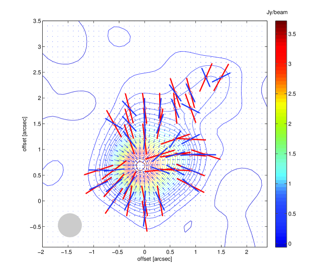
The W51 e2 map (Figure 1) analyzed in the following sections was obtained with the SMA interferometer (Tang et al., 2009). The observation was carried out at a wavelength of 0.87 mm where the polarization of dust thermal emission is traced. In the extended array configuration, the synthesized beam resolution was about $0\farcs 7$ with a primary beam (field of view) of about $30\arcsec$ at 345 GHz. A detailed description of the data analysis with a discussion and interpretation of the obtained images is given in Tang et al. (2009). The re-constructed features depend on the range of $uv$-sampling and weighting. Nevertheless, these data currently provide the highest angular resolution ($\theta$) information on the morphology of the magnetic field in the plane of sky obtained with the emitted polarized light in the W51 star formation site. This study is part of the program on the SMA (Ho et al., 2004) to study the structure of the magnetic field at high spatial resolutions.

W51 e2 is one of the strongest mm/submm continuum sources in the W51 region. Located at a distance of 7 kpc (Genzel et al., 1981), 1$\arcsec$ is equivalent to $\sim$ 0.03 pc. Chrysostomou et al. (2002) measured the polarization at 850$\mu$m with SCUBA on JCMT across the molecular cloud at a scale of 5 pc with a binned resolution $\theta\approx 9\farcs$3. At this scale, the polarization shows a morphology that changes from the dense cores to the surrounding diffuser gas. Lai et al. (2001) reported a higher angular resolution (3$\arcsec$) polarization map at 1.3 mm obtained with BIMA, which resolved out large scale structures. In contrast to the larger scale polarization map, the polarization appears to be uniform across the envelope at a scale of 0.5 pc, enclosing the sources e2 and e8. In the highest angular resolution map obtained with the SMA at 870 $\mu$m with $\theta\approx 0\farcs$7, the polarization patterns appear to be pinched in e2 and also possibly in e8 (Tang et al., 2009). In particular, the structure detected in the collapsing core e2 reveals hourglass-like features. A statistical analysis based on a polarization structure function (of second order) shows a turbulent to mean magnetic field ratio which decreases from the larger (BIMA) to the smaller (SMA) scales from $\sim 1.2$ to $\sim 0.7$ (Koch et al., 2010), possibly demonstrating that the role of magnetic field and turbulence evolves with scale. The apparent axis of the hourglass along the north-west south-east direction coincides with the axes of the bipolar outflows in CO(2-1) (Keto & Klaassen, 2008), CO(3-2) and HCN(4-3) (Shi et al., 2010). Collapse and/or accretion flow signatures, possibly orthogonal to that, have been reported for various molecules in Rudolph et al. (1990); Ho & Young (1996); Zhang & Ho (1997); Young et al. (1998); Zhang et al. (1998); Solins et al. (2004); Keto & Klaassen (2008). This might correspond roughly to the depolarization regions along the north-east south-west direction in Figure 1.

The highest resolution SMA map of W51 e2 serves as a testbed for the method developed in the following section. Figure 1 reproduces the dust continuum Stokes $I$ map with the magnetic field segments (red) from Tang et al. (2009). Detected polarization segments are rotated by 90^∘ in order to derive the field directions. Typical measurement uncertainties of individual position angles are in the range of $5^{\circ}$ to $10^{\circ}$. Additionally shown in the map are features relevant for the method in the following section.

3 Method

In this section we introduce a new method which allows us to measure the (projected) magnetic field strength in a molecular cloud as a function of the position in a map. Starting from an observed correlation in Section 3.1, the details of the method and its link to observed dust continuum Stokes $I$ and polarization maps are given in Section 3.2. We follow up with a qualitative analysis of the features of the method in Section 3.3.

3.1 Motivation: Magnetic Field – Intensity Gradient Correlation

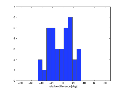
The Stokes $I$ dust continuum contours and the magnetic field segments (red) from the dust polarization emission (Tang et al., 2009) are shown in Figure 1 for W51 e2. Interestingly, field segments tend to be perpendicular to Stokes $I$ emission contours, or equivalently, polarization is preferentially tangential to the emission contour lines. Instead of further working with intensity contours, we alternatively choose to investigate the intensity gradients (blue thick segments in Figure 1). The top panel in Figure 2 displays the magnetic field position angles ($P.A.$s) versus the intensity gradient $P.A.$s. A close correlation becomes manifest. Both $P.A.$s are defined counter-clockwise starting from north in a range of 0 to 180^∘. The few data points (black empty squares) which originally do not seem to follow the trend, belong to pairs where both segments are close to $P.A.=0$ (vertical orientation), but with one of the $P.A.$s slightly rotated to the left and the other one slightly rotated to the right hand side of the vertical. Despite being closely correlated in orientation (small absolute differences), these pairs would mimic a bad correlation simply due to the definition of the $P.A.$s. For these cases, the original range of the magnetic field $P.A.$ (0 to 180^∘) is extended by adding their relative difference in $P.A.$s to their intensity gradient $P.A.$s. E.g., a pair with an intensity gradient and magnetic field $P.A.$ of 175^∘ and 5^∘ has a relative difference of 10^∘, and is therefore displayed as (175^∘,185^∘). This re-definition does not alter the correlation in any way, but is merely a consequence of the ambiguity in the conventional definition of the $180^{\circ}$ $P.A.$ range.

We note that the correlation is not limited to those pairs directly in the core collapsing region, but seemingly still holds for the most northern segments where the emission contours start to deviate from circular shapes. The correlation – in the definition of Pearson’s linear correlation coefficient – is 0.95. It is important to remark that, despite this tight correlation, the distribution of the differences (between magnetic field $P.A.$s and intensity gradient $P.A.$s) is non-Gaussian with an absolute mean of $\sim 20^{\circ}$. A KS-test rejects the null hypothesis (differences following a Gaussian distribution) with a $p-$value of $\sim 10^{-7}$. As a matter of fact, the relative differences show a bimodal distribution (bottom panel in Figure 2), which results from a systematic clockwise and counter-clockwise rotation of the magnetic field with respect to the intensity gradient. This further points toward a systematic origin of this correlation. All this leads to the conclusion that magnetic field and intensity gradient can not simply be radially aligned with the apparent misalignment just being the result of some measurement uncertainty. It is the focus of an on-going study where this correlation is further analyzed on a larger data sample in the context of the evolution of molecular clouds (Koch et al. 2012; in preparation).

In the following section, this observed correlation and the measured non-Gaussian differences in position angles of the magnetic field and the intensity gradient are further used to investigate the field strength.

3.2 MHD and Dust Polarization

3.2.1 Local Field Strength

Molecular clouds are the sites of interactions of various forces. Gravity, magnetic fields, expanding shells such as from expanding HII regions or supernovae, accretion and outflows all add to the dynamics, and their relative importance can vary with the evolutionary stage of the star formation site. Generally, magneto-hydrodynamics (MHD) equations - possibly for various molecules and dust with individual coupling terms - are needed to provide an accurate and complete description of the system. In the following, aiming at making use of dust polarization measurements, a single MHD equation for the dust component is adopted. Under the assumptions of negligible viscosity and infinite conductivity (ideal MHD case) we focus on the force equation:

$$\rho\left(\frac{\partial}{\partial t}+\mathbf{v}\cdot\mathbf{\nabla}\right)\mathbf{v}=-\mathbf{\nabla}\left(P+\frac{B^{2}}{8\pi}\right)-\rho\nabla\phi+\frac{1}{4\pi}\left(\mathbf{B}\cdot\mathbf{\nabla}\right)\mathbf{B},$$ (1)

where $\rho$ and $\mathbf{v}$ are the dust density and velocity, respectively. $\mathbf{B}$ is the magnetic field. $P$ is the hydrostatic dust pressure. $\phi$ is the gravitational potential resulting from the total mass contained inside the star forming region. $\mathbf{\nabla}$ denotes the gradient. As usual, the left hand side in Equation (1) describes the resulting action based on the force terms on the right hand side. These include the gradients of the hydrostatic pressure terms of the gas, the magnetic field and the gravitational potential together with the magnetic field tension term (last term on the right hand side).

In the following, an interpretation of Equation (1) is derived which can be matched to a polarization observation as in Figure 1. We start by noting that the magnetic field tension term, $\sim(\mathbf{B}\cdot\mathbf{\nabla})\mathbf{B}$, can be rewritten as:

$$\left(\mathbf{B}\cdot\mathbf{\nabla}\right)\mathbf{B}=B\frac{\partial B}{\partial s_{B}}\mathbf{e}_{s_{B}}+B^{2}\frac{\partial\mathbf{e}_{s_{B}}}{\partial s_{B}}=B\frac{\partial B}{\partial s_{B}}\mathbf{e}_{s_{B}}+B^{2}\frac{1}{R}\mathbf{n},$$ (2)

where a magnetic field line, $\mathbf{B}=B\mathbf{e}_{s_{B}}$, is directed along the unity vector $\mathbf{e}_{s_{B}}$ with the generalized coordinate $s_{B}$ along the field force line. A change in direction, $\partial\mathbf{e}_{s_{B}}/\partial s_{B}$, measures the magnetic field curvature $1/R$ and is directed normal to $\mathbf{e}_{s_{B}}$ along the unity vector $\mathbf{n}$. In an analogous way, $(\mathbf{v}\cdot\mathbf{\nabla})\mathbf{v}$ can be reformulated with the velocity vector $\mathbf{v}=v\mathbf{e}_{s_{v}}$ directed along the unity vector $\mathbf{e}_{s_{v}}$.

Generally, the gradient of the isotropic field pressure, $\sim\nabla\left(\frac{B^{2}}{8\pi}\right)$, in Equation (1) is not necessarily directed along the field direction $\mathbf{e}_{s_{B}}$, but can also have a component orthogonal to it. Therefore, when combining the Equations (2) and (1), a term $\sim B\frac{\partial B}{\partial s_{B_{\bot}}}\mathbf{e}_{s_{B_{\bot}}}$ remains which needs to be compared to the curvature term $\sim B^{2}\frac{1}{R}\mathbf{n}$. Both $\mathbf{n}$ and $\mathbf{e}_{s_{B_{\bot}}}$ are orthogonal to $\mathbf{e}_{s_{B}}$, but they are not necessarily collinear. Assuming $\partial s_{B_{\bot}}$ and $R$ to be given approximately by the resolution of an observation, the significance of this additional term can be estimated as $|B\frac{\partial B}{\partial s_{B_{\bot}}}|/\left(B^{2}\frac{1}{R}\right)\approx\frac{\Delta B_{\bot}}{B}\ll 1$. Thus, the term can be omitted if the local change in the normal field component, $\Delta B_{\bot}$, is small compared to the total field strength. This holds for any smooth and slowly varying function of field strength. Equation (1) can then be transformed into:

$$\rho v\frac{\partial v}{\partial s_{v}}\mathbf{e}_{s_{v}}+\rho v^{2}\frac{\partial\mathbf{e}_{s_{v}}}{\partial s_{v}}=-\frac{\partial P}{\partial s_{P}}\mathbf{e}_{s_{P}}-\rho\frac{\partial\phi}{\partial s_{\phi}}\mathbf{e}_{s_{\phi}}+\frac{1}{4\pi}B^{2}\frac{1}{R}\mathbf{n},$$ (3)

where the resulting directions of the gradients of pressure and gravitational potential are given with $\mathbf{e}_{s_{P}}$ and $\mathbf{e}_{s_{\phi}}$, respectively. In the above formulation, generalized coordinates $s_{v},s_{P},s_{\phi},s_{B}$ along the directions of the unity vectors $\mathbf{e}_{s_{v}},\mathbf{e}_{s_{P}},\mathbf{e}_{s_{\phi}},\mathbf{e}_{s_{B}}$ are used. Generally, these vectors are not collinear, but have different three-dimensional directions with the condition that the vector sum of the right hand side adds up to the resulting direction on the left hand side. Each term in Equation (3) is intentionally written with its corresponding unity vector, defining its specific direction. This will later be used when interpreting Equation (3) together with an observed map. Equivalently, all unity vectors can be expressed in any regular coordinate system (e.g. spherical coordinates $r$, $\theta$, $\phi$) should this be of advantage. The unity vectors $\mathbf{e}_{s_{v}},\mathbf{e}_{s_{P}},\mathbf{e}_{s_{\phi}},\mathbf{e}_{s_{B}}$ can be interpreted as volume averaged directions, where the size of a volume element will depend on the resolution of an observation. In the above derivation we have neglected the partial time derivative, $\partial/\partial t$, assuming stationarity.

Equation (3) describes the basic interaction of forces and the resulting motion. Linking some of these terms (in direction and strength) with observations will then allow us to solve for others. Our goal is to isolate the magnetic field strength $B$ in the term $\frac{1}{4\pi}B^{2}\frac{1}{R}\mathbf{n}$. Therefore, the remaining terms in Equation (3) need to be identified and characterized. Dust in star formation sites is reacting to all the force terms in Equation (3). Maps of observed dust emission are reflecting the overall result of gravity, pressure and magnetic field. Consequently, they represent a measure of the resulting motion, the left hand side in Equation (3). We make the fundamental assumption that a change in emission intensity is the result of the transport of matter driven by the combination of the above mentioned forces. Adopting this, it then follows that the gradient in emission intensity defines the resulting direction of motion on the left hand side in Equation (3). For the directions of the gradients of the pressure and the gravitational potential we assume here, for simplicity, a spherically symmetrical molecular cloud, where the center can be identified from the peak emission. This assumption is relaxed in Section 4, where the method is generalized to an arbitrary cloud shape.

It is important to remark that the derivation so far is generally valid for 3 dimensions. Projection effects in both the integrated Stokes $I$ and the polarized emission inevitably are present in an observation. In the following we first proceed by identifying Equation (3) with an observed map in 2 dimensions. Projection effects are later addressed in Section 6.2. Figure 3 illustrates the further steps. The derivation of $B$ is shown for a measured polarization (red) and intensity gradient direction (blue) in the first quadrant (with respect to the gravity center which here is supposed to coincide with the emission peak). For each measured pair of polarization and intensity gradient, its distance and direction from the gravity center defines the gravitational pull, $\rho\frac{\partial\phi}{\partial s_{\phi}}\mathbf{e}_{s_{\phi}}$. Generally, gravity, magnetic field and the intensity gradient directions are different. The schematic in Figure 3 illustrates how the vector sum of the various terms in Equation (3) is constructed. Solving for the magnetic field term then relies on measurable angles in the orientations between polarization and the intensity gradient ($\alpha$) and the difference between the gravity and the intensity gradient directions ($\psi$). Applying a sinus theorem to the closed triangle, $\frac{\nabla P+\rho\nabla\phi}{\sin\alpha}=\frac{\frac{1}{4\pi}B^{2}\frac{1}{R}}{\sin\psi}$, leads to the expression for the magnetic field strength:

$$B=\sqrt{\frac{\sin\psi}{\sin\alpha}\left(\nabla P+\rho\nabla\phi\right)4\pi R},$$ (4)

where, in the most general case, all variables are functions of positions in a map.

We note that – although illustrated for a simple, close to spherically symmetric case in Figure 3 with $\nabla P$ and $\rho\nabla\phi$ aligned and pointing toward the same center – Equation (4) is generally valid for any directions of $\nabla P$ and $\rho\nabla\phi$. Thus, the above derivation is not restricted to a spherical collapsing core, but can be applied to any configuration where the various local force directions can be identified (see also Sections 4 and 6.1).

3.2.2 Local Field Significance

As an important further outcome of the method, the angle factor $\frac{\sin\psi}{\sin\alpha}$ in Equation (4) has a direct physical meaning. With the magnetic field tension force term $F_{B}=\frac{B^{2}}{4\pi R}$ and the gravitational and pressure forces $|F_{G}+F_{P}|=|\rho\nabla\phi+\nabla P|$, Equation (4) can be reformulated as:

$$\left(\frac{\sin\psi}{\sin\alpha}\right)_{local}=\left(\frac{F_{B}}{|F_{G}+F_{P}|}\right)_{local}\equiv\Sigma_{B},$$ (5)

where we have introduced $\Sigma_{B}$ to define the field significance. This directly quantifies the local impact of the magnetic field force compared to the other forces involved (gravity and pressure gradient). Remarkably, the ratio is free of any model assumptions and simply relies on the two measured angles. It is purely based on the geometrical imprint by the various forces left in the field and intensity gradient morphologies. The angle factor, thus, also provides a model-independent qualitative criterion whether the magnetic field can prevent an area in a molecular cloud from gravitational collapse $(\Sigma_{B}>1)$ or not $(\Sigma_{B}<1)$. The field significance $\Sigma_{B}$ and its implications for the mass-to-flux ratio and the star formation efficiency are investigated in Koch et al. (2012).

3.3 Qualitative Analysis

We briefly illustrate the expected features of our method when applied to a representative field and intensity configuration in a molecular cloud (Figure 4). A summary is given in Table 1. Field lines like (I) and (II) are expected in a core collapse when gravity is dragging inward the magnetic field which is flux-frozen to the dust particles. In the case of (I), the field line is close to the pole, little bent, and the gas is mostly moving along the field. Intensity gradients are mostly radial, pointing toward the center of gravity. Therefore, in the outer region (a), $R\approx$ const, $\delta$ small ($\sin\alpha\approx 1$), $\psi$ small ($\sin\psi\approx\psi\approx$ const) and thus $\Sigma_{B}\approx$ const. The field strength $B$ will scale as $\sim r^{-\kappa}$, where $\kappa>0$ describes a power-law profile resulting from density and gravitational potential gradient (Section 5.3). Small (random) changes in angles are possible due to local turbulence and can lead to some scatter. In the inner part (b), $R$ might slightly decrease with the other parameters remaining roughly constant. This will lead to similar scalings for $\Sigma_{B}$ and $B$. A field line of type (II) is expected around the accretion direction. The outer field (a) is still little bent ($R\approx$ const), $\delta\approx$ const and small, $\psi$ small, and therefore $\Sigma_{B}\approx$ const and $B\sim r^{-\kappa}$ as in (Ia). In (b) the field lines start to bend more significantly ($R$ decreases) and $\delta$ increases ($\sin\alpha$ decreases). $\psi$ is small ($\approx$ const) or possibly increasing if a a non-spherical central core is being formed. Thus, $\Sigma_{B}$ can increase as $\sim\frac{1}{\sin\alpha}$. The field strength is additionally modulated by $\sqrt{\frac{R}{\sin\alpha}}$ which can lead to a steeper or shallower profile than $r^{-\kappa}$ depending on the exact values of $R$ and $\alpha$. In the most inner section (c), the field radius is minimized, field and intensity gradient directions are close to orthogonal to each other ($\delta\sim\frac{\pi}{2}$ modulo some turbulent dispersion, $\alpha\sim 0$), and $\psi$ is small. The force ratio $\Sigma_{B}$ can then possibly further increase locally. The field strength is thus mostly controlled by $\sqrt{\frac{1}{\sin\alpha}}$ and the power-law exponent $\kappa$, which will lead to highest values here. Overall, for (I) and (II) we thus expect the field strength to generally increase with smaller radius toward the center.

Additional features are seen in Figure 1, which are possibly not directly linked to the above cases. Region (III) – corresponding to the NE patch around the offset (-0.3,1.8) – shows a group of parallel B field segments with parallel intensity gradients. In this outer region the collapse is likely initiated, but does not yet reveal clear signatures. $\psi$ is changing, $\delta\approx$ const ($\sin\alpha\approx$ const), $R\approx$ const, and $\Sigma_{B}$ can therefore increase or decrease. The field strength will generally be small here because of the low density. The relative field significance can still be important here, as gravity has not yet fully taken control to shape and align intensity gradient and field direction. Area (IV) corresponds to the most northern part in Figure 1. This region is possibly disconnected from the main core, likely belonging to another smaller core being formed here. The $\Sigma_{B}$ values are dominated by large changes in $\psi$ when linked to the gravitational center of the main core. Due to the lack of a clear identification of a local gravity center (in which case $\psi$ would be much smaller), $\Sigma_{B}$ is probably overestimated for the two most northern segments. Possible solutions to this issue are addressed in Section 4.2. The field strength is again small here due to the low density.

4 Generalizing to Arbitrary Cloud Shapes

This section focuses on the 2 remaining parameters in Equation (4), which are not yet explicitly locally evaluated: the magnetic field radius $R$ (curvature $C\equiv 1/R$) and the gravitational potential $\phi$. In particular, the initial assumption of a spherically symmetrical molecular cloud from Section 3 is given up. It has to be stressed that the method in Section 3 derived from the Equation (1) remains unchanged, and is valid for both average or locally precise values in $R$ and $\phi$.

4.1 Local Curvature

From the derivation in Section 3, both angles $\alpha$ and $\psi$, the gravitational potential and the pressure $P$ are generally functions of positions $(x,y)$ in a projected plane of sky map. The magnetic field line radius $R$ (curvature $C\equiv 1/R$) will generally also change with positions. It is, however, not possible to define a curvature based on a single isolated polarization segment. For polarization observations with a sufficiently large number of segments (as e.g. in Figure 1), a curvature resulting from two adjacent (or more) polarization segments can be calculated.

Two neighboring magnetic field segments, separated by distance $d$, are assumed to be tangential to a field line of radius $R$. The difference in their position angles, $\Delta PA$, is a measure of how much the direction of the field line has changed over $d$. The curvature $C$ can then be written as (Figure 5):

$$C\equiv\frac{1}{R}=\frac{2}{d}\cos\left(\frac{1}{2}\left[\pi-\Delta PA\right]\right).$$ (6)

With this definition of a local curvature, the calculation of the field strength $B$ in Equation (4) is no longer limited to an average field curvature, but can be precise to any locally varying field structure.

We remark that the above definition for $C$ is not necessarily unique. In particular, determining which segments connect to a field line can be non-trivial. Additionally, for some neighboring segments, as it can also be seen in Figure 1, it is obvious that they can not be both tangential to the same field line. The curvature as defined in Equation (6) is therefore rather a local averaged curvature. In this view, a local curvature can not only be defined with two segments which are roughly lining up, but also with two segments side by side. The local field radius map in Figure 6, middle left panel, is calculated by averaging the local curvatures between two adjacent segments over all available closest neighbors. A closest neighbor is defined through the grid spacing of the map. Depending on the resolution and the detection of a polarization structure, the definition of $C$ can possibly be adjusted or refined.

For W51 e2, the local field radius derived from Equation (6) is in the range between $\sim 1\arcsec$ and $\sim 17\arcsec$ (Figure 6, middle panels). Whereas most areas in the map show rather uniform patches with $R\sim 1\arcsec-3\arcsec$, regions in the north-east and south-west around the accretion plane show larger radii. This is possibly a consequence of the accretion flow which tends to align field lines until some limiting inner radius where the field will bend. Yet more likely, this is a boundary effect because only two almost parallel segments are available here for averaging. This leads to unphysically large radii. The local radius averaged over the map is $<R>\approx 3\farcs 3$. Discarding the extreme values gives $<R>\approx 1\arcsec$.

4.2 Local Gravity Direction

Unless the gas distribution in a molecular cloud is (close to) perfectly symmetrical in azimuth around an emission peak, $\nabla\phi$ will differ in direction and strength from a simple radius-only dependence in the gravitational potential. Thus, for an arbitrary mass distribution, the direction and strength of the local gravitational pull, $\rho\frac{\partial\phi}{\partial s_{\phi}}\mathbf{e}_{s_{\phi}}$ in Equation (3), can not any longer simply be constructed with the direction and distance to the reference center (emission peak in Figure 1). Instead, at any position in a map, the distribution of all the surrounding mass has to be taken into account to calculate the resulting local gravitational force. Since the method in Section 3 is based on measuring angles between various force directions (including gravity) at all positions in a map, any substantial local deviations from a simple global gravity model can be relevant.

For a discrete mass distribution ($m_{i}$), the resulting total potential $\phi$ at a location $\mathbf{r}$ is: $\phi(\mathbf{r})=-G\sum^{n}_{i=1}\frac{m_{i}}{|\mathbf{r}-\mathbf{r}_{i}|}$, where $G$ is the gravitational constant. We assume that a detected dust emission (like in Figure 1) is proportional to the gravitating mass, and that it further traces reasonably well the overall gravitating potential. Additionally, it is assumed that the dust temperature is roughly constant over the emission map. In this case, there is no weighting for $m_{i}$ when linking it to the integrated dust emission $I_{i}$. The local gravity force (per unit mass), $\mathbf{g}(\mathbf{r})=-\nabla\phi(\mathbf{r})$ is then:

$$\mathbf{g}(\mathbf{r})=G\sum^{n}_{i=1}\frac{I_{i}\cdot f_{i}}{|\mathbf{r}-\mathbf{r}_{i}|^{2}}\cdot\mathbf{e}_{i},$$ (7)

where $f_{i}$ is a conversion factor linking dust emission and total mass, and $\mathbf{e}_{i}$ is the direction between each detected position with dust emission ($\mathbf{r}_{i}$) and the local position ($\mathbf{r}$) where the gravity force is evaluated.

We remark that, if $f_{i}\equiv f$ over the entire map, the local gravity direction can be derived without prior knowledge of $f$. For a typical observation, the mass (intensity) distribution is obtained by pixelizing a map with the beam resolution. Figure 6, bottom left panel, shows the deviations from an azimuthally symmetrical potential for W51 e2 when calculating the local gravity directions following Equation (7) for $f_{i}\equiv f$. This analysis shows that, although W51 e2 (Figure 1) appears to be a rather spherically symmetrical collapsing core, the deviations are systematically positive or negative on one or the other side of the hourglass axis. Minimum deviations are roughly along the south-east north-west direction which is consistent with the hourglass axis. The average absolute deviation is $\approx 9^{\circ}$. As further discussed in the Sections 6.4 and 6.5, already this simple symmetry analysis points toward a systematic influence of the magnetic field.

These deviations provide a correction for the angle $\psi$ (angle between the gravity direction and the intensity gradient, Figure 3), which originally is calculated assuming an azimuthally symmetrical potential (Figure 7, top left panel). Consequently, also the magnetic field strength $B$ in Equation (4) needs to be recalculated. The angle $\alpha$, as defined relative to the intensity gradient, remains unchanged with this local gravity correction.

We finally note that further refinement of the local gravity correction introduced here is possible. Local over-densities – which follow the flow of the global dynamics – can eventually locally collapse once they pass the Jeans mass. The north-west extension in Figure 1 is possibly such a case. Using Equation (7), however, the resulting local gravity direction will always be dominated by the main mass (emission). Consequently, the angle $\psi$ might be over- or underestimated. This defect can be corrected by identifying local collapse centers with a local maxima search and a suitable threshold criterion.

5 Results

This section applies the method developed in Section 3 to the case of W51 e2. Starting from the expression for the magnetic field strength $B$ in Equation (4), results are first presented for separated factors and then for the final field strength. Whereas in the original observed map in Figure 1 the magnetic field is gridded to half of the synthesized beam resolution, the maps in the following are interpolated for an enhanced visual impression. This can emphasize features along the field lines where polarization is detected at equally separated spacings. On the other hand, it might lead to non-physical values in depolarization zones along the south-west north-east direction or in the center, where no data are available.

5.1 Angle Factors

5.1.1 $\sin\psi$ – map

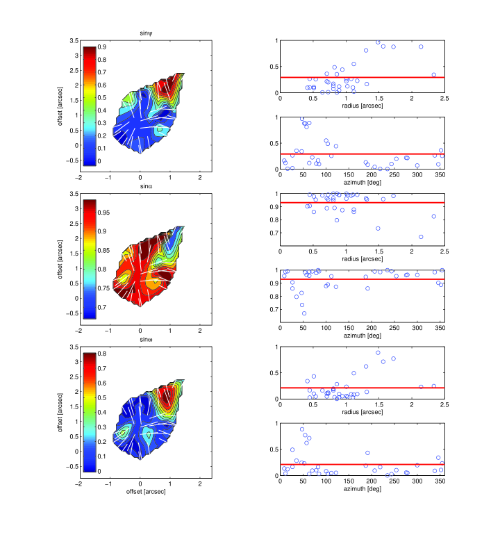
The angle $\psi$ measures the difference between the orientations of the intensity gradient and gravity. Small values in $\psi$ (or $\sin\psi$) therefore indicate that a change in the local intensity structure is closely following global gravity. The top panels in Figure 7 show a map of $\sin\psi$ together with its trends as a function of radius and azimuth. The peak emission (Figure 1) is again assumed as the reference center, and the gravity direction is simply taken as the radial direction from the center to any measured intensity location. Small values of $\sin\psi$ - in the range between 0 and 0.2 - are found for most of the magnetic field segments pointing toward the center. An X-pattern is revealed made up from the majority of the segments. There is a trend of larger $\sin\psi$ values in the north-east and south-west where likely accretion is ongoing. The magnetic field segments in the far north show $\sin\psi$ values close to one. Here, the intensity gradient directions are very different (by up to 90^∘) from the global gravity directions. This northern patch, therefore, seems to be decoupled from the main collapsing core (Section 3.3, case (IV)). $\sin\psi$ averaged over the entire map gives $<\sin\psi>\approx 0.29$ ($<\psi>\approx 20^{\circ}$). The average decreases to about 0.19 ($<\psi>\approx 12^{\circ}$) if the six polarization segments in the far north are ignored. A hint of an increase in $\sin\psi$ with radius is apparent in the top right panel in Figure 7. Again, the most northern patch dominates values beyond a distance of $\sim 1.5\arcsec$. No clear structure in azimuth is revealed.

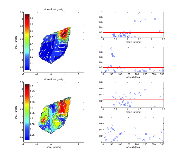
Since $\psi$ measures a deviation from gravity, mass distributions differing from an azimuthal symmetry can introduce corrections to the local gravity direction (Section 4.2). The top left panel in Figure 8 displays the $\sin\psi$ – map calculated from the generalized gravitational potential in Equation (7). The overall patterns are still similar to the uncorrected $\sin\psi$ – map, but with smaller values in the accretion areas. As a result, the average is reduced to $<\sin\psi>\approx 0.19$ ($<\psi>\approx 12^{\circ}$) and to about 0.09 ($<\psi>\approx 6^{\circ}$) when discarding the most northern patch.

5.1.2 $\sin\alpha$ – map

The difference in orientations between the intensity gradient and the magnetic field is denoted with $\delta$ (Figure 3). The angle $\alpha$ is its complement to 90^∘. Or, in other words, $\alpha$ is the difference in orientations between a measured (projected) polarization and the intensity gradient. Values of $\alpha$ close to its maximum of 90^∘ ($\sin\alpha\approx 1$), indicate that the projected magnetic field orientation and the intensity gradient are closely aligned. This again reflects the initially presented correlation in Section 3.1. The middle panels in Figure 7 show a map of $\sin\alpha$ with its radial and azimuthal dependence. Around the collapsing core, the values of $\sin\alpha$ are between 0.85 and 1. They decrease to about 0.7 in the most northern area. The intensity and magnetic field orientations are therefore very similar over most of the map, with an average value $<\sin\alpha>\approx 0.93$ ($<\alpha>\approx 72^{\circ}$). Leaving out the most northern part gives $<\sin\alpha>\approx 0.95$ ($<\alpha>\approx 74^{\circ}$). Possibly there is a slight trend of decrease in $\sin\alpha$ with radius. No clear structures appear in azimuth. $\alpha$ is not affected by local gravity corrections as outlined in Section 4.2.

5.2 Magnetic Field Force Compared to Other Forces

The angle factor $\left(\frac{\sin\psi}{\sin\alpha}\right)_{local}=\left(\frac{F_{B}}{|F_{G}+F_{P}|}\right)_{local}\equiv\Sigma_{B}$ measures in a model-independent way the local impact of the magnetic field force (Section 3.2.2). The top panels in Figure 6 illustrate the results. Values for the relative field significance, $\Sigma_{B}$, range from $\sim 0.1$ to $\sim 1.3$, with an average over the entire map $<\Sigma_{B}>\approx 0.33$. Thus, the magnetic field can balance only about one third of the gravitational force. Consequently, it can not prevent the core from any further collapse. We stress that this result is obtained without any assumption about the mass involved. The top panels in Figure 6 further show that the impact of the magnetic field changes as a function of position. Generally, the field influence seems to become weaker toward the center where gravity likely becomes more and more dominant. This result is further explored in Koch et al. (2012).

5.3 Magnetic Field Strength Maps

Maps for the magnetic field strength $B$ are presented in this section for two scenarios: Firstly, only the newly introduced force ratio $\Sigma_{B}$ is taken into account, leaving the other parameters in Equation (4) constant. This will illustrate the influence of $\Sigma_{B}$. Secondly, the field strength is calculated by combining $\Sigma_{B}$ together with an analysis of the density profile and the resulting gravitational potential. A first order estimate of the field strength, comparing the gravitational force $F_{G}=\frac{GM_{R}\rho}{R_{G}^{2}}$ and the magnetic field tension $F_{B}=\frac{B^{2}}{4\pi R_{B}}$ is given in Tang et al. (2009). Since W51 e2 is a collapsing core, $F_{G}>F_{B}$, an upper limit of the field strength, $B<19$ mG, can be derived. $M_{R}(\approx 220~{}M_{\odot})$ refers to the gas mass enclosed within a radius $R_{G}(\approx 1\arcsec)$. The radius of a magnetic flux tube is $R_{B}(\approx 1\arcsec)$. The mass density $\rho$ is estimated with the gas volume number density $n_{H_{2}}(\approx 2.7\times 10^{7}$ cm${}^{-3})$. $G$ is the gravitational constant. The above value, $B<19$ mG, will serve as a reference for the magnetic field strength maps presented in the following. We remark that Equation (4) is consistent with the above estimate, $B=\sqrt{4\pi R_{B}G\frac{M_{R}\rho}{R_{G}^{2}}}=\sqrt{4\pi R_{B}\rho\nabla\phi}$, when setting $\frac{\sin\psi}{\sin\alpha}=1$ and neglecting the pressure gradient $\nabla P$.

In the first scenario, the $B$ map for W51 e2 is calculated by taking into account only the angles $\psi$ and $\alpha$. Field radius, potential and density are set constant as above. Assuming local changes in temperature and density to be negligible compared to gravity, the pressure gradient $\nabla P$ is omitted from Equation (4) in the following. From the measured ranges in $\psi$ and $\alpha$ (Figure 7, $\sin\psi\approx 0.1-0.9$, $\sin\alpha\approx 0.7-1$), it is then obvious that mostly $\psi$ will dominate the range and structure in a magnetic field strength map (Figure 9). Values of the factor $\frac{\sin\psi}{\sin\alpha}=\Sigma_{B}$ range from $\sim 0.1$ to $\sim 1.3$, with an average over the entire map $<\Sigma_{B}>\approx 0.33$ (Figure 6, top panels). The resulting patterns are very similar to the ones in the $\sin\psi$-map (Figure 7, top left panel). Resulting variations in $B$ are then from a few mG to $\approx 20$ mG. The map average value is $<B>\approx 10$ mG. Compared to the reference value above, the correction factor $\frac{\sin\psi}{\sin\alpha}$ generally leads to a lower field strength. Discarding the most northern patch – where $B$ is likely overestimated due to the lack of a clear local gravity center (Section 3.3) – the value becomes $<B>\approx 8$ mG. Obviously, when leaving curvature, gravitational potential and density constant, the radial profile of the field strength is determined by $\Sigma_{B}^{1/2}$. As the field-to-gravity force ratio decreases toward the center, consequently the field strength also decreases and its largest values tend to be in the outer zones (Figure 9). This result needs to be compared with the following complete analysis.

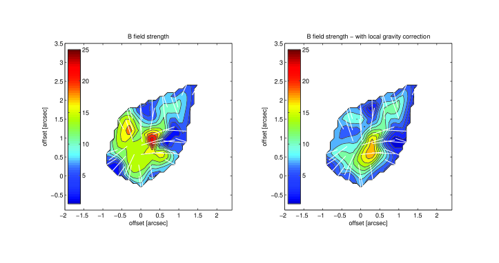
In the second scenario, the field strength is calculated by additionally taking into account the profiles of density and gravitational potential. As discussed later in Section 6.2, the force ratio $\Sigma_{B}$ is little or not at all affected by projection effects. Therefore, we proceed to reconstruct 3-dimensional radial profiles assuming spherical symmetry. For that purpose, the azimuthally averaged dust emission profile from Figure 1 is deprojected with an Abel integral. The resulting 3-dimensional radial profile ($r$) is well described with a functional form $f(r)\sim\frac{1}{(r+0.35)^{3}}$, whereas the initial projected map ($R$) is well fit with a profile $\sim\frac{1}{(R+0.25)^{2}}$. The fitting is performed on profiles with values binned to half of the synthesized beam resolution. Assuming the total mass of the e2 core to be distributed similar to its dust component, the cumulative mass $m(r)\sim\int_{0}^{r}f(r^{\prime})\,4\pi r^{\prime 2}\,dr^{\prime}$ and the resulting gradient of the potential $\sim\frac{m(r)}{r^{2}}$ can be derived. Combining all together (Equation(4)), the magnetic field strength profile scales as $B(r)\sim\left(\Sigma_{B}(r)\cdot f(r)\cdot\frac{m(r)}{r^{2}}\right)^{1/2}$. Whereas the dust emission map allows us to derive this functional form, its absolute normalization remains to be determined. Adopting $<\Sigma_{B}>\approx 0.33$ (Section 5.2) – i.e. the observed averaged magnetic field strength can balance only about one third of the gravitating mass $M_{R}(\approx 220~{}M_{\odot})$ – we normalize $B$ so that $<B^{2}>=<\Sigma_{B}>\cdot(19~{}mG)^{2}$, where the latter field strength is equivalent to $220~{}M_{\odot}$ (Tang et al., 2009). This gives $<B>\approx 9.4~{}$mG. The final field strength map and its radial and azimuthal trends are shown in the left panels in the Figures 10 and 11. An increase in field strength with smaller radius becomes apparent. A profile $\sim r^{-1/2}$ is overlaid for illustration. A hint of an increase in field strength around $r\approx 1.5\arcsec$ possibly points toward the forming core in the northwest. This is found by still assuming a dominating gravity center at the emission peak. It is obvious that the first map (Figure 9) can not represent the correct field strength, but merely reflects the relative field significance. Only by adding profiles for the density and the gravitational potential can the magnetic field profile correctly be derived. Density and gravitational potential only (setting $\Sigma_{B}\equiv 1$) would lead to a field profile $\sim r^{-1.7}$. Taking into account the decreasing field-to-gravity force ratio with radius, leads to the shallower scaling $B(r)\sim r^{-1/2}$. With the density profile, $\rho\sim r^{-3}$, this connects field and density as $B(r)\sim\rho^{1/6}$. Whereas the dust emission shows little variations in azimuth (close to spherical symmetry), the local position-dependent measurement of $\Sigma_{B}$ shows some variations. Consequently, features in the magnetic field strength map start to be revealed, with possibly regions of increased strength in the accretion zones in the north-east and the south-west directions. In order to trace the magnetic field to the very center, higher resolution observations will be needed.

We remark that the projected dust emission can also reasonably well, although with larger residuals, be fit with a $\sim R^{-1}$ profile. The deprojected profile $f(r)\sim\frac{1}{(r+0.25)^{2}}$ then gives a magnetic field profile $B(r)\sim r^{-0.3}$ and $B(r)\sim\rho^{3/20}$ (not shown). This leads to about 15% lower values in the field strength in the center with a similar mean field strength $<B>\approx 9.8~{}$mG. All the other features are left unchanged. In the above final field strength map we have neglected the variations in the field radius and assumed it to be constant (Figure 6, top panels). This ignores two zones where large field radii are likely a consequence of boundary effects (Section 4.1).

Finally, the influence of the local gravity correction is illustrated in the right panels in the Figures 10 and 11. Generally, features tend to be smoother. The field strengths in the accretion zones are less pronounced and a single center becomes apparent. The average strength is about 7.7 mG. The radial profile of the binned values remains close to $B(r)\sim r^{-1/2}$ with maximum values around 19 mG. Structures in azimuth remain similar although with smaller variations.

We stress that, although we are making use of the total gravitating mass $M_{R}$ – which sets an upper limit for the field strength and defines its order of magnitude – only the newly derived force ratio $\Sigma_{B}$ leads to a proper normalization and opens the possibility to derive a radial profile. This has become possible by solving the MHD force equation by the method introduced in Section 3.2.

Errors $\Delta B$ in the final $B$ field maps are estimated by propagating typical measurement uncertainties through Equation (4). The individual polarization $P.A.$ uncertainty of $5^{\circ}$ to $10^{\circ}$ is assumed for $\Delta\alpha$. A slightly smaller uncertainty, $\sim 3^{\circ}$ to $5^{\circ}$, can be expected for $\Delta\psi$ because of the averaging process in the interpolation when calculating the intensity gradient. This leads to $\Delta B\approx\pm\frac{1}{2B}(4\pi R\rho\nabla\phi)\cdot 0.05$, where the numerical factor follows from the above uncertainties combined with map averaged values for $<\sin\alpha>$ and $<\sin\psi>$. For any of the above scenarios and $<B>\approx 9$ mG, we derive an average systematic error $<\Delta B>_{sys}\approx\pm 1$ mG. Errors in the profiles for density and gravitational potential are small after binning and azimuthal averaging. They are, therefore, neglected here. Besides this systematic error, there is an additional statistical uncertainty in the field orientation resulting from the turbulent field dispersion. Adopting $5^{\circ}$ to $10^{\circ}$ for this (Koch et al., 2010), this contributes to the final error budget with $<\Delta B>_{stat}\approx\pm 1$ mG. We note that all uncertainties in angles are smaller than the mean value ($\approx 20^{\circ}$) of the differences between magnetic field and intensity gradient $P.A.$s (Section 3.1). This further confirms that the correlation in Figure 2 can not only result from systematic and statistical uncertainties.

In conclusion, density and gravitational potential profiles determine the order of magnitude of the field strength. The local features result from the angle factor $\frac{\sin\psi}{\sin\alpha}$. These features remain robust with typical total errors (systematic and statistical) of $\Delta B\approx\pm(1-2)$ mG. The derived field strengths are also consistent with the level of magnetic fields typically detected by Zeeman effects on OH masers in compact HII regions (a few mG up to $\sim 20$ mG, Fish & Reid (2007)).

6 Discussion

6.1 Comparison, Application Regime and Limitations of the Method

The method presented in Section 3 leads to a local magnetic field strength. It, nevertheless, uses strictly speaking a not exactly local but larger scale property of the field, namely its curvature (Figure 5). The shape of a field line is the result of various forces acting on the dust particles coupled to the magnetic field. These can be both long-ranging forces (like gravity) as well as locally acting perturbations (like turbulence). In order to solve Equation (1), we need to determine the larger scale curvature. The locally turbulent field can here act as a contaminant. This is in contrast to, e.g. the CF method which precisely uses the field dispersion around an average field direction, in combination with some turbulent velocity information, to derive a magnetic field strength. In principle, a curvature can be calculated from a minimum of two segments (Section 4.1), but the local turbulent field can introduce some uncertainty here. Assuming an isotropic turbulent field component, a local curvature can be derived by averaging over several neighboring curvatures. As long as reasonably smooth and connected polarization patterns are detected, this will reveal the larger scale field curvature. This is the case for the field morphology in Figure 1 where a clear signature of dragged-in field lines is apparent. Higher resolution data are then needed to trace the field in the inner most part of the collapsing cloud where the curvature is expected to change faster within a small area.

The method further relies on identifying a noticeable effect from the various forces in Equation (1) which shape the field on large scales. When assuming flux freezing, this means that $B^{2}/(8\pi)<P_{gas}+\rho\phi+\rho v^{2}$. In this weak field case of flux-freezing, the field lines are forced to move along with the gas (at least up to some scale where ambipolar diffusion sets in). As a consequence, gravity, intensity gradient and field orientations can be individually determined which is needed to calculate the angles in Equation (4). In the strong field case, $B^{2}/(8\pi)\gg P_{gas}+\rho\phi+\rho v^{2}$, where matter can mostly move only along field lines, the method will yield $\psi\sim 0$, $\alpha\sim\pi/2$, $R\rightarrow\infty$, and therefore $B\rightarrow\infty$. (see also Section 3.3.) Unless the pressure gradient $\nabla P$ can be identified, which then allows to measure $\psi\neq 0$, the method can not further constrain $B$ (see also Table 1). Geometrically, the method is based on closing a force triangle (Figure 3). Thus, if $\psi\sim 0$ or $\alpha\sim 0$ or if both angles are zero at the same time, the triangle is no longer defined and the method fails.

In summary, whereas the CF method is based on the field dispersion but has to isolate a mean large-scale field direction, the method discussed here uses the large-scale field morphology shaped by various forces. Therefore, the method is more directly applicable to the weak field case. A successful extension to the strong field case is possible if pressure and/or gravitational potential gradients can be localized. Generally, coherent patches with smooth changes in field and intensity gradient directions are of advantage as this leads to a clear identification of the field curvature and the acting forces. The CF method needs both dust polarization continuum and molecular line velocity observations. The method here uses the dust continuum Stokes $I$ and its polarized emission. Whereas the CF method provides one single statistically averaged value, the approach here leads to a map of field strength values.

Finally, we conclude this section by noting that the method here is not limited to dust continuum polarization. As long as a force triangle can be identified, the method is applicable to any measurement which reveals the large-scale field morphology in combination with gravity and/or pressure forces. Notably, molecular cloud polarization maps obtained from the Goldreich-Kylafis (GK) effect, i.e. from spectral line linear polarization (Goldreich & Kylafis, 1981, 1982), can be analyzed in the same way. This might open a way to study outflows which are often not observed in dust continuum due to their relatively small masses. The only complication possibly rises from the difficulty that it can be non-trivial to conclude whether the magnetic field is parallel or perpendicular to the polarization detected from the GK effect. In an even broader context, the method introduced here can also be applied to field morphologies detected from polarization by synchrotron emission or from Faraday rotation measures. The method is, therefore, not limited to molecular clouds, but can potentially also be adopted for, e.g. galaxy rotation measures.

6.2 Projection Effects

The results in Section 5 were derived assuming the plane of sky projected geometry in Figure 3. Here, we address the question of how an original 3-dimensional configuration affects the parameters in Equation (4) to calculate the magnetic field strength. The schematic in Figure 13 illustrates the connection. We note, that like in the 2-dimensional (2D) case, gravitational pull (and pressure gradients), magnetic field tension and the resulting intensity gradient have to form a closed triangle. The projected 2D triangle can generally be deprojected with 2 different inclination angles: $\iota_{a}$ and $\iota_{b}$, corresponding to the inclinations of the deprojected orientations of the magnetic field tension and the gravitational pull, respectively.

Strictly speaking, projection effects are likely to be present to some extent in all variables in Equation (4). Having deprojected the intensity emission profile and adopted an average field radius (Section 5.3), we limit the discussion to the remaining factor $\frac{\sin\psi}{\sin\alpha}$. In the following, lower indices ’3’ or ’2’ refer to 3-dimensional or 2-dimensional projected quantities. The deprojection of the side $b_{2}$ of the triangle (Figure 13) can be written as $b_{3}=\sqrt{b_{2}^{2}+\pi_{b}^{2}}$ and $\tan\iota_{b}=\frac{\pi_{b}}{b_{2}}$, where $\pi_{b}$ is the length of the projection along the line of sight ($z$-direction). Analogous relations hold for the side $a_{2}$. Linking a sinus theorem in the 3D triangle, $\frac{\sin\psi_{3}}{\sin\alpha_{3}}=\frac{a_{3}}{b_{3}}$, to the previously used 2D expression $\frac{\sin\psi_{2}}{\sin\alpha_{2}}=\frac{a_{2}}{b_{2}}$, then yields:

$$\frac{\sin\psi_{3}}{\sin\alpha_{3}}=\frac{\sin\psi_{2}}{\sin\alpha_{2}}\cdot\sqrt{\frac{1+\tan^{2}\iota_{a}}{1+\tan^{2}\iota_{b}}}=\frac{\sin\psi_{2}}{\sin\alpha_{2}}\cdot\frac{\cos\iota_{b}}{\cos\iota_{a}}$$ (8)

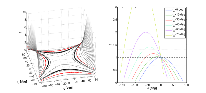
where $\iota_{a},\iota_{b}\in[-\pi/2,\pi/2]$. It becomes obvious that for any inclination angles, the projection effects cancel out as long as gravitational pull ($\iota_{b}$) and field tension ($\iota_{a}$) are inclined by the same angles, i.e. $\iota_{a}\equiv\iota_{b}$. Furthermore, if $\iota_{a}$ and $\iota_{b}$ are different, projection effects are negligible as long as $\iota_{a}$ and $\iota_{b}$ are small. For $\iota_{a}$ and $\iota_{b}$ within about $\pm 40^{\circ}$, the projection effect is within about $\pm 20$%. The left panel in Figure 14 displays the relevant function $f(\iota_{a},\iota_{b})=\frac{\cos\iota_{b}}{\cos\iota_{a}}$, which shows a large relatively flat saddle around one in the center. For extreme values, i.e. inclination angles $|\iota_{a}|,|\iota_{b}|>75^{\circ}$, the projection effect becomes severe ($f\rightarrow 0$ or $f\rightarrow\infty$). Besides having two totally different inclination angles $\iota_{a}$ and $\iota_{b}$, we also investigate the projection effect as a function of the difference between the two inclination directions, $\Delta=\iota_{b}-\iota_{a}$ (Figure 14, right panel). Since the gravitational pull and the field tension directions are dynamically coupled, their inclination angles are likely to be not completely independent. The right panel in Figure 14 shows that projection effects are within about $\pm 30$% for a range in the differences $\Delta$ up to about 100^∘ or more, up to inclinations of about $\pm 45^{\circ}$. For larger inclinations $f$ grows again. These situations, however, might not be of a concern, because at such large inclinations of the field lines, polarization emission (perpendicular to the field lines) might not be detectable. The analysis might, therefore, not be applicable.

In summary, for identical inclination angles projection effects cancel out. The effect is small (up to $\sim 30$%) or even negligible for one inclination up to $\sim 45^{\circ}$ and the other one varying within about $+50^{\circ}$ and $-50^{\circ}$ (range in $\Delta$ up to about $100^{\circ}$). Only for extreme inclinations larger than about $75^{\circ}$ projection effects can severely affect the method. Such situations might, however, not be detectable. It, thus, has to be emphasized that it is unlikely that severe projection effects are present if regular polarization patterns are observed. Consequently, the method introduced here leads to a total magnetic field strength.

6.3 Shortcomings of the Method

Without any further modeling, the method does not include components such as e.g., rotation or temperature variations. Effects due to rotation are not explicitly considered in Equation (1). Nevertheless, an additional term due to rotation on the right hand side of Equation (1) would primarily lead to a change in the resulting direction of motion, $\rho v\frac{\partial v}{\partial s_{v}}\mathbf{e}_{s_{v}}+\rho v^{2}\frac{\partial\mathbf{e}_{s_{v}}}{\partial s_{v}}$ in Equation (3), which was identified with the intensity gradient direction. Technically, this is equivalent to an additional inclination in the intensity gradient and can thus be approximated as a projection effect. Similarly, the directions of the magnetic field lines dragged along with the rotating gas would be subject to an additional projection effect. As discussed in Section 6.2, the resulting uncertainty in the field strength is relatively small for a large parameter space of inclination angles. Alternatively, if the rotation velocity and axis are known, Equation (1) could be written in a rotating frame with an additional contribution from a centrifugal force.

Density and temperature combined make up for the detected dust emission. Significant variations in temperature could mimic mass concentrations which might then lead to wrong gravity directions and, therefore, to wrong magnetic field strength values. If concentrated locally such as e.g., in the case of radiation pressure from a star, this is unlikely to alter the global features in the field strength over an entire map. Similarly, small shifts in the position of a dominating emission peak (like in Figure 1) introduce only minor variations in the field strength. Only if there are very irregular and significant changes in temperature over a map, the method is likely to fail. Additional information (such as from spectra) might then help to isolate the temperature effect.

6.4 Dynamical Importance of the $B$ Field: Flux-Freezing and the Magnetic Field - Intensity Gradient Relation

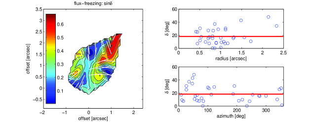
Following up on Section 6.1, we expect the strong and weak field case of flux-freezing to be present with different characteristics. In the strong field case – gas moving along the field lines – the intensity gradient direction is presumably closely aligned with the magnetic field orientation. On the other hand, in the weak field case – field lines dragged along and shaped by the forces acting on the gas – intensity gradient and field orientations can be at any angle. In the extreme case they can be at a 90^∘ angle, when e.g. a gas flow is bending a field line (case (IIc) in Figure 4). The angle $\delta(=\pi/2-\alpha)$, as previously introduced in Figure 3, measures the absolute difference in orientations between the intensity gradient and the magnetic field. Since the cases of weak and strong flux-freezing categorize the relative importance of the field, we propose here the angle $\delta$ as a diagnostic measure for the dynamical role of the $B$ field. Small angles ($\sim 0$) will point toward a dominating field, whereas larger and larger angles mean that the field is being overwhelmed by other forces.

The map in Figure 12 displays $\delta$, revealing some areas with $\delta\approx 0$. These areas roughly coincide with the expected hourglass at larger radii. Here, the gas is possibly collapsing along the field lines. Additionally, it is likely that gravity has initially led to this field and intensity gradient configuration, with $\delta\approx 0$ being a mere consequence of that. Both at smaller radii toward the center and away from the hourglass toward the accretion plane, values for $\delta$ increase. This might be an indication that the field is dynamically less important here and that gravity has largely taken control. It needs to be stressed that this does not necessarily mean that the field strength is smaller here, because $B$ further also depends on $R$, $\nabla\phi$ and $\nabla P$ (see also previous footnote). Moreover, the field can still provide pressure support which can slow down the gravitational collapse. This picture – with generally smaller $\delta$ values around the core and larger values toward the north-west corner – is consistent with the angle factor $\frac{\sin\psi}{\sin\alpha}$ (Section 3.2.2 and top panels in Figure 6), which identifies the field force to be less significant in the core. Figure 12 is necessarily complementary to the middle panels in Figure 7, because $\delta=\pi/2-\alpha$.

We have to note that the angle $\delta$ (like $\alpha$) is subject to a projection correction. In the notation of Section 6.2: $\delta_{3}=\pi/2-\alpha_{3}$ with $\sin\alpha_{3}=\frac{\sin\psi_{3}}{\sin\psi_{2}}\cdot\sin\alpha_{2}\cdot f^{-1}(\iota_{a},\iota_{b})$. In the particular case of a close to spherical collapse, $\frac{\sin\psi_{3}}{\sin\psi_{2}}\approx 1$, because both the 3-dimensional and the projected intensity show a clear azimuthal symmetry (Figure 1). Assuming $f(\iota_{a},\iota_{b})$ to be approximately constant over a map (Section 6.2), then gives $\sin\alpha_{3}\approx const\cdot\sin\alpha_{2}$. Thus, despite the projection effect, the dynamical importance of the field can still be understood from the relative differences in $\delta$. The significance of the angle $\delta$ as a diagnostic measure is further analyzed on a larger data set together with the correlation from Section 3.1 in Koch et al., 2012 (in preparation).

6.5 Magnetic Field and Gravity Alignment: $\sin\omega$ – map

The method developed in Section 3 is based on identifying the three orientations of gravity, the magnetic field and the emission intensity gradient. In particular, two angles are relevant in order to isolate and calculate the magnetic field strength $B$: the angle $\psi$ between the gravity direction and the intensity gradient, and the angle $\alpha$ between the polarization orientation and the intensity gradient. Given the three orientations, an additional angle, $\omega$, can be read off from a map. $\omega$ measures the difference in orientations between gravity and the magnetic field (Figure 3). Thus, it is a measure for how effectively gravity is able to shape the field lines and aligning them with the direction of the gravitational pull. Small angles (small values of $\sin\omega$) indicate close alignment. The bottom panel in Figure 7 shows $\sin\omega$ for the case of W51 e2, assuming the center of gravity to be at the emission peak. The bottom panels in Figure 8 display again $\sin\omega$ when a local gravity direction (Section 4.2) is adopted. The two figures are qualitatively similar. Applying a local gravity direction seems to sharpen the contrasts. The closest alignment ($\sin\omega\approx 0.1-0.2$) is found at the outer radii close to the accretion plane in the west and in the north-west direction around the axis of the hourglass-like structure. An obvious poor alignment is in the northern area. Averaged over the entire map and excluding the northern patch we derive $<\sin\omega>\approx 0.21$ ($<\omega>\approx 13^{\circ}$) and $<\sin\omega>\approx 0.14$ ($<\omega>\approx 8^{\circ}$), respectively. Interestingly, after the local gravity correction, there is a very close resemblance between the $\sin\omega$-map and the $\sin\delta$-map (Figure 12). Since $\omega$ measures the magnetic field - gravity alignment and $\delta$ measures the magnetic field - intensity gradient alignment, the very similar maps, of course, indicate that the intensity structure is mostly resulting from gravity. This is also shown with the small values in the $\sin\psi$-map (Figure 8, top panels). This is, of course, a consequence of the geometry in Figure 3 because all the 3 angles are dependent: $\omega=\pi/2-\alpha-\psi$ with $\alpha=\pi/2-\delta$. Nevertheless, the clear systematic differences in structures between the $\sin\omega$ and the $\sin\psi$-map (Figure 8) lead to the conclusion that the $B$ field – at least in some regions – has kept its own dynamics and is not yet aligned and overwhelmed by gravity. This result is then also consistent with the finding of zones of weak and strong flux-freezing (Section 6.4) which characterizes the dynamical role of the magnetic field. The systematic influence of the field is further manifest in the systematic deviations from an azimuthally symmetric emission structure, seen in the bottom panels in Figure 6. Projection effects (Section 6.2) are again likely to change only the absolute numbers, leaving relevant features and comparisons between maps still intact.

7 Summary and Conclusion

Dust polarization observations in molecular clouds often show position angles of magnetic field segments which are close to perpendicular to the dust continuum intensity contours. This correlation does not seem to be arbitrary, but can be interpreted in the context of ideal magneto-hydrodynamics (MHD). Based on this, we put forward a new method to derive a local magnetic field strength. The key points are summarized in the following.

1. New method for magnetic field strength mapping: A new method is proposed which leads to a position-dependent estimate of the magnetic field strength. The approach is based on measuring the angle between the polarization and the Stokes $I$ intensity gradient orientations. Assuming that the intensity gradient is a measure for the resulting direction of motion in the MHD force equation, this angle quantifies how tightly the direction of motion is coupled to the field orientation. In combination with the angle in between the orientations of gravity (and/or the pressure gradient) and the intensity gradient, the two angles can be linked to the field strength by identifying a force triangle.

2. Application regime: The method relies on separating noticeable effects from various components in the MHD force equation, in particular from gravitational pull and field tension. Consequently, the method is more directly applicable to the case of weak field flux freezing, where the field morphology is clearly shaped by these forces. Collapsing (spherical) cores in star formation sites are of most immediate interest because the directions of gravity and magnetic field are relatively easily determined. Nevertheless, the technique is generally valid and applicable to any measurement (also strong field flux freezing), where the directions of magnetic field, pressure gradients and/or gravitational pull can be localized. With the concepts of local curvature and local gravity direction, the method can be further generalized. Moreover, the method is not limited to dust polarization measurements, but can potentially also be applied to, e.g. molecular line linear polarization maps from the GK effect or even to Faraday rotation measure maps for galaxies.

   Here, the method is applied to SMA dust polarization data of the collapsing core W51 e2. Averaging over the entire core, a field strength of $\sim 7.7$ mG is found. Variations in the field strength are detected with an azimuthally averaged radial profile $B(r)\sim r^{-1/2}$. Maximum values toward the center are about $19$ mG. The current data lack resolution in order to probe the innermost part of the core, where the largest field strength is expected.

3. Comparison with Chandrasekhar-Fermi (CF) method: The method introduced here uses the large-scale field curvature. The local turbulent field dispersion is acting as a contaminant. This is in contrast to the CF method which precisely uses the field dispersion – after separating a mean field orientation – in combination with a turbulent velocity information in order to derive a field strength. Whereas the CF method yields one statistically averaged field strength for an ensemble of polarization segments, the method here provides a field strength at each location of a detected polarization segment.

4. Limitations and shortcomings of the method: Technically, the method fails where the force triangle can not be closed. This leads to the unphysical value $B\rightarrow\infty$. A triangle degenerating to a single line corresponds to the situation where the field is very weak and, therefore, the intensity gradient does not deviate from the gravity direction. The method then still consistently yields the limit $B\rightarrow 0$.

   The method is not entirely free of projection effects. In the most general case, the force triangle has to be deprojected with two different inclination angles. Nevertheless, the projection correction enters as the ratio of the two inclination angles. Thus, in the most favorable case with identical inclination angles for gravity and field orientations, the projection effect cancels out and the method leads to a total magnetic field strength. Even if the inclination angles differ from each other, the possible error due to unknown inclinations is relatively modest, within $\pm 30$% to $\pm 50$%, for a large parameter space. In any case, if the inclination angles do not vary significantly within the same source, the method always provides a way to detect relative differences in the field strength. The accuracy and reliability of the method are limited by how well projection effects and forces defining the field morphology can be identified and quantified. Additional effects like, e.g. rotation and local variations in temperature are likely of minor importance.

5. Weak and strong flux freezing: The dynamical role of the magnetic field – in the sense of weak or strong flux freezing – can be assessed through the angle between the magnetic field and the intensity gradient orientations. Angles close to zero point toward a dominating role of the field (or an overall controlling gravitational pull). Larger angles indicate that the field lines are more significantly shaped by other forces. Although this criterion alone does not constrain the field strength, it provides a measure to characterize the role of the magnetic field as a function of position in a map.

6. Dynamical significance of magnetic field: The method additionally provides a model-independent criterion to quantify the magnetic field force compared to the sum of any other forces involved. As a result of the force triangle, the local significance of the magnetic field can be evaluated simply with the ratio of the angle between intensity gradient and gravity direction, and the angle between intensity gradient and polarization orientation. These angles reflect the imprint of the various forces onto the dust and polarization morphologies. This measure can then constrain the local impact of the magnetic field and quantify its support against gravitational collapse.

The authors thank the referee for valuable comments which led to further significant insight in this work. P.T.P.H. is supported by NSC grant NSC97-2112-M-001-007-MY3.

Figure 1: The collapsing core W51 e2 (Tang et al., 2009). Contours show the Stokes $I$ dust continuum at 0.87 mm with a synthesized beam resolution of about $0\farcs 7$ (gray ellipse in the lower left corner) with natural weighting. Colors correspond to the color wedge on the right hand side with units in Jy/beam. Contours are linearly spaced in steps of 130 mJy/beam. Overlaid are the magnetic field segments (thick red segments) at the locations where polarized emission was detected. Magnetic field segments are plotted by rotating the polarization segments by 90^∘. Only polarization data with a flux above $3\sigma_{I_{p}}$, the rms noise of the polarized intensity, are included. The blue vector field displays the gradient directions of the dust continuum emission, with most vectors pointing toward the emission peak. Highlighted are those emission intensity gradient directions (thick blue segments) at the locations of the magnetic field segments. The length of the segments is arbitrary, and for visual guidance only. The axes offset positions (in arcsec) are with respect to the original phase center of the observation at Right Ascension (J2000)= $19^{\rm h}23^{\rm m}43^{\rm s}.95$, Declination (J2000)=$14^{\circ}30\arcmin 34\farcs 00$

Figure 2: Top panel: the correlation (blue filled squares) between the intensity gradient $P.A.$s (blue segments in Figure 1) and the magnetic field $P.A.$s (red segments in Figure 1). The black empty squares belong to pairs with $P.A.$s close to $P.A.=0$, one $P.A.$ being slightly rotated to the left and the other one to the right hand side of the vertical. In order to properly display their correlations, the magnetic field $P.A.$ is re-defined beyond the 0 to 180^∘ range for these cases (blue filled squares above 180^∘ and below 0^∘). For visual guidance added is the straight blue line, representing a perfect correlation. Also shown are the absolute differences ($\leq 90^{\circ}$) between the $P.A.$s for each pair (red crosses). Both $P.A.$s are defined counter-clockwise starting from north. Bottom panel: the bimodal distribution of the relative differences (in the range between $-90^{\circ}$ to $+90^{\circ}$) between the intensity gradient and the magnetic field $P.A.$s, reflecting a systematic clockwise and counter-clockwise rotation of the field with respect to the intensity gradient.

Figure 3: Illustration of the Equation (4) with the relevant angles in order to solve for the magnetic field strength $B$. A pair of magnetic field (red solid line) and emission intensity gradient segments (blue solid line) are shown at a location $(\Delta x,\Delta y)$ with respect to a common reference center. The originally measured polarization orientation (rotated by 90^∘ with respect to the field orientation) is indicated as a red dashed line. Position angles are measured counter-clockwise with respect to north (N). $\delta\leq\pi/2$ measures the angle in between the intensity gradient and the field orientation. $\alpha$ is its complement to $\pi/2$. $(\nabla P+\rho\nabla\phi)$ are assumed to be known in direction and strength. For simplicity, as suggested from Figure 1 for the case of W51 e2, the emission peak is assumed as the gravity center, and thus defines direction and strength. Here, it also serves as the reference center. $\psi$ denotes the deviation of the intensity gradient from the direction of $(\nabla P+\rho\nabla\phi)$. The corresponding deviation for the magnetic field is measured with the angle $\omega$. The force triangle – $(\nabla P+\rho\nabla\phi)$ pointing toward the gravitating center, the resulting intensity gradient orientation (left hand side in Equation (3)) and the direction of the restoring magnetic field tension (normal to the field segment) – can then be closed by intercepting the red dotted and black dotted lines, where the former one is shifted parallel to the red dashed line.

Figure 4: Qualitative analysis (Section 3.3): Illustration of the expected features of the method. The black solid lines are intensity emission contours. Blue and red segments are intensity gradient and magnetic field orientations, respectively, as in the Figures 1 and 3. The labeling refers to the cases discussed in Section 3.3 and listed in Table 1. All cases have similar equivalents in the W51 e2 map in Figure 1.

Figure 5: Illustration of the local curvature derivation. Position angles ($P.A.$s), separated by an observed distance $d$, are measured counter-clockwise with respect to north (N). The 2 magnetic field segments (solid red lines) are assumed to be tangential to a connecting field line (thick solid black line) with radius $R$. The angle $\xi$ measures the difference in between 2 $P.A.$s, $\xi=|P.A._{1}-P.A._{2}|\equiv\Delta P.A.$. $R$ is read from the isosceles triangle with $\cos\gamma=\frac{d/2}{R}$, where $\gamma=\frac{\pi}{2}-\beta=\frac{1}{2}(\pi-\Delta P.A.)$. This then leads to Equation (6). Note that the derivation uses the measured relative quantities $d$ and $\Delta P.A.$. Technically, this allows to detach the magnetic field segments from their absolute positions, by keeping their relative separation and $\Delta P.A.$, and ensures that a connecting field line can be constructed. Strictly speaking, even this definition of curvature is not exactly local because it involves at least 2 segments separated by a distance $d$.

Figure 6: Position dependence of parameters in Equation (4). Magnetic field segments are shown in white. Top left panel: the combined factor $\frac{\sin\psi}{\sin\alpha}=\Sigma_{B}$, which quantifies the significance of the magnetic field force compared to the other forces (Section 3.2.2). $\psi$ is measured with respect to a spherically symmetrical gravitational potential. Middle left panel: the local magnetic field radius calculated from the method in Section 4.1. Units are in arcsec. Bottom left panel: the difference in the direction of the gravitational pull between a spherically symmetrical potential and a local gravity direction as defined in Section 4.2. Units are in degree. The difference is shown relative to the symmetrical assumption, revealing a symmetry axis along the southeast- northwest direction. The right panels illustrate the tendencies for $\Sigma_{B}$, $B$ field radius and difference in gravity direction (from top to bottom) as a function of radius (distance from emission peak) and azimuth angle (measured counter-clockwise from west). Mean values averaged over the entire maps are shown with the red solid lines. For the local gravity difference the mean is calculated from the absolute differences.

Figure 7: Relevant angles for the derivation of the magnetic field strength, calculated for W51 e2 (Figure 1). Magnetic field segments are shown in white. Top left panel: $\sin\psi$-map, where $\psi$ $(\leq\pi/2)$ (Figure 3) is the difference between the orientations of the intensity gradient and gravity. Middle left panel: $\sin\alpha$-map. $\pi/2-\alpha$ $(\leq\pi/2)$ measures the deviation between the magnetic field and the intensity gradient orientations. Bottom left panel: $\sin\omega$-map, where $\omega$ is the difference between the magnetic field and gravity orientations. The right panels show the corresponding tendencies for each angle as a function of radius (distance from emission peak) and azimuth angle (measured counter-clockwise from west). Mean values averaged over the entire maps are shown with the red solid lines.

Figure 8: Angles corrected for local gravity directions. Magnetic field segments are shown in white. Top panels: $\sin\psi$ measuring the deviation between the local gravity and the intensity gradient orientations. Bottom panels: $\sin\omega$ measuring the deviation between the local gravity and the magnetic field orientations.

Figure 9: The magnetic field strength (B) derived by taking into account only variations in the field-to-gravity force factor $\frac{\sin\psi}{\sin\alpha}\equiv\Sigma_{B}$. Units are in mG. All the other parameters in Equation (4) are constant over the map. Magnetic field segments are shown in white. The right panels show the field strength tendencies as a function of radius (distance from emission peak) and azimuth angle (measured counter-clockwise from west). Mean values averaged over the entire map are shown with the red solid lines.

Figure 10: Final magnetic field strength maps calculated from Equation (4). Units are in mG. Taken into account are the deprojected profile for the density, the resulting gravitational potential gradient profile and variations in the force ratio $\Sigma_{B}$ (left panel). In the right panel, corrections due to the local gravity direction are additionally considered. Mean field strengths are about 9.4 mG and 7.7 mG for the left and right map, respectively. The field radius is set constant. Magnetic field segments are shown in white. Typical measurement uncertainties lead to an average systematic error in the field strength of $<\Delta B>_{sys}\approx\pm 1$ mG.

Figure 11: Radial and azimuthal trends for the magnetic field strength maps presented in Figure 10. Radial profiles $\sim r^{-1/2}$ are overlaid for illustration in the top panels. Mean values averaged over the entire map are shown with the red solid lines.

Figure 12: The angle $\delta$ (absolute difference in between the intensity gradient and the magnetic field orientations (Figure 3)) as a diagnostic tool to distinguish between weak and strong case of flux-freezing. Magnetic field segments are shown in white. The values for $\sin\delta$ are displayed in the left panel in order to facilitate a comparison with the $\sin\alpha$ (Figure 7, middle panels) and the $\sin\omega$ maps (Figure 7, bottom panel; Figure 8, bottom panel).

Figure 13: Projected and deprojected triangles for the method presented in Section 3. Lower indices ’3’ or ’2’ refer to 3-dimensional or 2-dimensional projected quantities. The projected triangle (dashed lines) in the $xy$-plane is deprojected along $\pi_{b}$ and $\pi_{a}$ (parallel to the line of sight) to form a 3D triangle (solid lines). The angles $\psi_{2}$ and $\alpha_{2}$ are identical to $\psi$ and $\alpha$ in Figure 3. $\iota_{b}$ and $\iota_{a}$ are the inclination angles of the gravitational pull and the magnetic field tension, respectively.

Figure 14: Left Panel: The projection function $f(\iota_{a},\iota_{b})=\frac{\cos\iota_{b}}{\cos\iota_{a}}$ for the two inclination angles $\iota_{a}$ and $\iota_{b}$ (Figure 13). The relatively flat saddle in the center shows that projection effects are small ($f\sim 1$) for $\iota_{a}$ and $\iota_{b}$ within about $\pm 40^{\circ}$. Highlighted in black and red are the parameter spaces where the projection effects are within $\pm 30$% ($f$ within $1\pm 0.3$) and within $\pm 50$% ($f$ within $1\pm 0.5$), respectively. For much larger inclination angles polarization is not easily detectable. It is, thus, unlikely that severe projection effects are present if regular polarization patterns are observed. Right Panel: The projection effect as a function of the difference $\Delta$ between the two inclination directions, $\Delta=\iota_{b}-\iota_{a}$, for various fixed inclinations $\iota_{a}$. The dashed line marks $f\equiv 1$. A $\pm 30$% bound is shown with the dotted lines.

Table 1: Qualitative Analysis

	$\psi$	$\alpha$	$R$	$\Sigma_{B}$	$B$	Comments
General
	$\downarrow\uparrow$	$\neq 0$	$R$	$\downarrow\uparrow$	$\downarrow\uparrow$, $\sim\sqrt{\sin\psi\cdot R}\cdot r^{-\kappa}$	$\Sigma_{B}$ and $B\uparrow$ with larger angle $\psi$
	$\neq 0$	$\downarrow\uparrow$	$R$	$\uparrow\downarrow$	$\uparrow\downarrow$, $\sim\sqrt{\frac{R}{\sin\alpha}}\cdot r^{-\kappa}$	$\Sigma_{B}$ and $B\uparrow$ with smaller angle $\alpha$
Specific Cases
(I) (a)	small, $\approx$ const	$\sim\frac{\pi}{2}$	$\approx$ const	$\approx$ const	$\approx$ const$\cdot r^{-\kappa}$	field line close to pole, $\Sigma_{B}\approx$ const, $B\uparrow$ with smaller $r$
(b)	small, $\approx$ const	$\sim\frac{\pi}{2}$	$\approx$ const	$\approx$ const	$\approx$ const$\cdot r^{-\kappa}$
(II) (a)	small, $\approx$ const	$\sim\frac{\pi}{2}$	$\approx$ const	$\approx$ const	$\approx$ const$\cdot r^{-\kappa}$	field line around accretion direction, $\Sigma_{B}\approx$ const, $B\uparrow$ with smaller $r$
(b)	small, $\approx$ const	$\downarrow$	$\downarrow$	$\sim\frac{1}{\sin\alpha}$	$\sim\sqrt{\frac{R}{\sin\alpha}}\cdot r^{-\kappa}$	$\Sigma_{B}\uparrow$, $B\uparrow$ with smaller $r$ steeper or shallower than $r^{-\kappa}$ (depending on $R$ and $\alpha$)
(c)	small, $\approx$ const	$\downarrow$, $\sim 0$	$\downarrow$, $R_{min}$	$\sim\frac{1}{\sin\alpha}$	$\sim\sqrt{\frac{R}{\sin\alpha}}\cdot r^{-\kappa}$	$\Sigma_{B}\uparrow$, maximum field strength $B$
(III)	$\uparrow\downarrow$	$\approx$ const	$\approx$ const	$\uparrow\downarrow$	$\uparrow\downarrow$, $\sim\sqrt{\sin\psi}\cdot r^{-\kappa}$	outer area, no clear signatures yet, $B$ generally small due to $r^{-\kappa}$
(IV)	large	$\approx$ const	$\approx$ const	large	$\sim\sqrt{\sin\psi}\cdot r^{-\kappa}$	disconnected area, no clear gravity center localized, $B$ small due to $r^{-\kappa}$
Limits
	$\rightarrow 0$	$\neq 0$	(i) $R^{1}$, (ii) $\rightarrow\infty^{2}$	$\rightarrow 0$	(i) $\rightarrow 0^{1}$, (ii) $\rightarrow\infty^{2}$	triangle degenerates to single line
	$\neq 0$	$\rightarrow 0$	(i) $R$, (ii) $\rightarrow\infty$	$\rightarrow\infty$	(i) $\rightarrow\infty$, (ii) $\rightarrow\infty$	method fails, triangle not closed
	$\rightarrow 0$	$\rightarrow 0$	(i) $R$, (ii) $\rightarrow\infty$	$\rightarrow$1	(i) $\sim\sqrt{R}$, (ii) $\rightarrow\infty$	method fails, triangle not closed and degenerated to single line

Note. — Qualitative analysis of the force ratio $\Sigma_{B}=\frac{\sin\psi}{\sin\alpha}$ and the magnetic field strength $B=\sqrt{\frac{\sin\psi}{\sin\alpha}\rho\nabla\phi\cdot 4\pi R}$ (Section 3.3). The pressure gradient is neglected here. The profile of the density and the resulting gradient of the gravitational potential is represented with $r^{-\kappa}$ with $\kappa>0$ (Section 5.3). The specific cases labeled (I) to (IV) refer to Figure 4. The cases (Ib), (IIb) and (IIc) are not yet observed due to the lack of higher resolution data. Down-arrows ($\downarrow$) and up-arrows ($\uparrow$) indicate decreasing and increasing values, respectively. ’$\approx$const’ indicates that small local variations can occur which lead to some scatter in $\Sigma_{B}$ and $B$ (Figure 11). Failure of the method – triangle can not be closed – refers to Figure 3 .

References

- Beuther et al. (2010) Beuther, H., Vlemmings, W.H.T., Rao, R., & van der Tak, F.F.S. 2010, ApJ, 724, L113
- Chandrasekhar & Fermi (1953) Chandrasekhar, S., & Fermi, E. 1953, ApJ, 118, 113
- Cho & Lazarian (2005) Cho, J., & Lazarian, A. 2005, ApJ, 631, 361
- Chrysostomou et al. (2002) Chrysostomou, A., Aitken, D.K., Jenness, T., et al. 2002, A&A, 385, 1014
- Cudlip et al. (1982) Cudlip, W., Fruniss, I. King, K.J., & Jennings, R.E. 1982, MNRAS, 200, 1169
- Cortes et al. (2008) Cortes, P.C., Crutcher, R.M., Shepherd, D.S., & Bronfman, L. 2008, ApJ, 676, 464
- Crutcher et al. (2009) Crutcher, R.M., Hakobian, N., & Troland, T.H. 2009, ApJ, 692, 844
- Draine & Weingartner (1996) Draine, B.T., & Weingartner, J.C. 1996, ApJ, 470, 551
- Draine & Weingartner (1997) Draine, B.T., & Weingartner, J.C. 1997, ApJ, 480, 633
- Falceta-Gonçalves et al. (2008) Falceta-Gonçalves, D., Lazarian, A., & Kowal, G. 2008, ApJ, 679, 537
- Fish & Reid (2007) Fish, V.L., & Reid, M.J., 2007, ApJ, 670, 1159
- Genzel et al. (1981) Genzel, R., Downes, D., Schneps, M.H., et al. 1981, ApJ, 247, 1039
- Girart et al. (2006) Girart, J.M., Rao, R., & Marrone, D.P. 2006, Science, 313, 812
- Goldreich & Kylafis (1981) Goldreich, P., & Kylafis, N.D. 1981, ApJ, 243, 75
- Goldreich & Kylafis (1982) Goldreich, P., & Kylafis, N.D. 1982, ApJ, 253, 606
- Heitsch et al. (2001) Heitsch, F., Zweibel, E. G., Mac Low, M.-M., Li, P., & Norman, M. L. 2001, ApJ, 561, 800
- Hildebrand et al. (1984) Hildebrand, R.H., Dragovan, M., & Novak, G. 1984, ApJ, 284, L51
- Hildebrand (1988) Hildebrand, R.H. 1988, Q.Jl R. astr. Soc., 29, 327
- Hildebrand et al. (2000) Hildebrand, R.H., Davidson, J.A., Dotson, J.L., et al. 2000, PASP, 112, 1215
- Hildebrand et al. (2009) Hildebrand, R.H., Kirby, L., Dotson, J.L., Houde, M., & Vaillancourt, J.E. 2009, ApJ, 696, 567
- Ho & Young (1996) Ho, P.T.P., & Young, L.M. 1996, ApJ, 472, 742
- Ho et al. (2004) Ho, P.T.P., Moran, J.M., & Lo, K.-Y. 2004, ApJ, 616, 1
- Houde (2004) Houde, M. 2004, ApJ, 616, L111
- Jokipii & Parker (1969) Jokipii, J.R., & Parker, E.N., 1969, ApJ, 155, 799
- Keto & Klaassen (2008) Keto, E., & Klaassen, P., 2008, ApJ, 678, L109
- Kirby (2009) Kirby, L. 2009, ApJ, 694, 1056
- Koch et al. (2010) Koch, P.M., Tang, Y.-W., & Ho, P.T.P. 2010, ApJ, 721, 815
- Koch et al. (2012) Koch, P.M., Tang, Y.-W., & Ho, P.T.P. 2012, ApJ, accepted
- Kudoh & Basu (2003) Kudoh, T., & Basu, S. 2003, ApJ, 595, 842
- Lai et al. (2001) Lai, S.-P., Crutcher, R.M., Girart, J.M., & Rao, R. 2001, ApJ, 561, 864L
- Lazarian (2000) Lazarian, A. 2000, ASPC, 215, 69
- Lazarian & Hoang (2007) Lazarian, A., & Hoang, T. 2007, MNRAS, 378, 910
- McKee & Ostriker (2007) McKee C. F., & Ostriker E. C., 2007, ARA&A, 45, 565
- Myers & Goodman (1991) Myers, P.C., & Goodman, A.A., 1991, ApJ, 373, 509
- Ostriker et al. (2001) Ostriker E. C., Stone J. M., & Gammie C. F., 2001, ApJ, 546, 980
- Padoan et al. (2001) Padoan, P., Goodman, A. A., Draine, B. T., et al. 2001, ApJ, 559, 1005
- Rao et al. (2009) Rao, R., Girart, J.M., Marrone, D.P., Lai, S.-P., & Schnee, S. 2009, ApJ, 707, 921
- Rudolph et al. (1990) Rudolph, A., Welch, W. J., Palmer, P., & Dubrulle, B. 1990, ApJ, 363, 528
- Schleuning (1998) Schleuning, D.A., 1998, ApJ, 493, 811
- Shi et al. (2010) Shi, H., Zhao, J.-H., & Han, J.L., 2010, ApJ, 718, L181
- Solins et al. (2004) Sollins, P. K., Zhang, Q., & Ho, P.T.P., 2004, ApJ, 606, 943
- Tang et al. (2009) Tang, Y.-W., Ho, P.T.P., Koch, P.M., et al. 2009, ApJ, 700, 251
- Troland & Crutcher (2008) Troland, T.H., & Crutcher, R.M. 2008, ApJ, 680, 457
- Young et al. (1998) Young, L. M., Keto, E., & Ho, P.T.P., 1998, ApJ, 507, 270
- Zhang & Ho (1997) Zhang, Q., & Ho, P.T.P., 1997, ApJ, 488, 241
- Zhang et al. (1998) Zhang, Q., Ho, P.T.P., & Ohashi, H., 1998, ApJ, 494, 636
- Zweibel (1990) Zweibel, E.G., 1990, ApJ, 362, 545