Entanglement and the Interplay between Staggered Fields and Couplings

Abstract

We investigate how the interplay between a staggered magnetic field and staggered coupling strength affects both ground state and thermal entanglement. Upon analytically calculating thermodynamic quantities and the correlation functions for such a system, we consider both the global Meyer-Wallach measure of entanglement and the concurrence between pairs of spins. We discover two quantum phase transitions present in the model and show that the quantum phase transitions are reflected in the behaviour of the entanglement at zero temperature. We discover that increasing the alternating field and alternating coupling strength can actually increase the amount of entanglement present at both zero temperature and for thermal states of the system.

I Introduction

Entanglement is an intriguing concept in quantum information, and a resource used in many quantum computation schemes manybody . The Heisenberg coupling in spin chains has been shown to allow universal quantum computation Divi . Spin chains are also good candidates for quantum wires Bose . Thus it is an important task to explore how the amount of entanglement in such systems changes under different conditions, to discover whether it can be enhanced and what causes its destruction.

Many-body entanglement manybody is difficult to quantify, so entanglement measures are often restricted to the pure, zero temperature case, for example von Neumann entropy Bennett or the Meyer-Wallach measure MW2002 , or to a small number of possibly mixed qubits such as concurrence OConnor . On the other hand, it is, in general, hard to quantitatively study the entanglement of thermal states due to the absence of efficient separability criterion for mixed states in many-body systems. An alternative approach is to use an entanglement witness which detects rather than measures entanglement. In particular, a thermodynamic entanglement witness uses thermodynamic quantities derived from the partition function of the system to detect entanglement ent_wit ; vlat .

In spin chains, ground state entanglement is often investigated in the context of quantum phase transitions (QPTs). A QPT is a sudden change in the properties of the ground state when a parameter of the Hamiltonian such as a magnetic field is varied. Since it is expected that by investigating QPTs, dramatic changes to physical quantities at very low temperature would be revealed, QPTs have been intensely studied in spin systems Sachdev . In Ref. WSL2004 , it was shown that in general, a singularity occurs in the ground state entanglement at quantum critical points (QCPs).

In this paper, we investigate the entanglement of a spin system in a non-uniform magnetic field with non-uniform coupling constants. Certain solid state systems such as Copper Benzoate have a non-uniform magnetic field Oshikawa , caused by an inhomogeneous Zeeman coupling. Similarly, examples exist for a non-uniform coupling strength Abraham ; Pincus . Some properties of these materials can be captured using the staggered spin chain we study in this paper.

Entanglement in a staggered magnetic field has been studied previously using single-site entropy and an entanglement witness StagHide . The effect of such a staggered field on the dynamics and on the high-fidelity transfer of entanglement has also been considered Crooks ; it was found that the staggered field is almost as efficient as the uniform case. On the other hand, entanglement in a spin chain with staggered coupling and magnetic field has been considered only numerically for chains of finite length Doronin .

Here, we show how to calculate two measures of entanglement analytically for such spin chains with infinite length. We first calculate thermodynamic properties and finite temperature correlation functions of the spin chain. Using these results, we show that the system exhibits QPTs at zero temperature induced by the staggered fields. We investigate global entanglement of the ground state using the Meyer-Wallach measure, a measure of multipartite pure states based on bipartite entanglement. We then investigate both zero and finite temperature entanglement between two spins using the concurrence. We find that global entanglement in general increases with an alternating coupling constant. At zero temperature, the concurrence first increases, reaches a maximum, then decreases with an alternating coupling constant. We also find that for certain values of magnetic field, both the Meyer-Wallach measure and the zero temperature concurrence can be increased by the alternating magnetic field. At finite temperature, the concurrence can again be increased by certain values of the staggered fields and couplings. Further, we examine the entanglement at finite temperature using an entanglement witness in view of searching for thermal multipartite entanglement.

This paper is organized as follows. In Section II, we present the Hamiltonian and give its diagonal form, which allows us to calculate thermodynamical quantities of the system. We compute the correlation functions in Section III. In Section IV, we investigate the ground state and show that the Hamiltonian exhibits QPTs. Then, we investigate entanglement at zero temperature and at finite temperature in Section V. We present concluding remarks in Section VI.

II The Hamiltonian and its thermodynamic properties

We consider the thermodynamic limit of the staggered Hamiltonian

$$H=-\sum_{l=1}^{N}\left[\frac{J_{l}}{2}\left(\sigma_{l}^{x}\sigma_{l+1}^{x}+\sigma_{l}^{y}\sigma_{l+1}^{y}\right)+B_{l}\sigma_{l}^{z}\right],$$ (1)

where $J_{l}=J+e^{i\pi l}j$ is the staggered coupling strength and $B_{l}=B+e^{i\pi l}b$ is the staggered magnetic field. We refer to $j$ as the alternating coupling strength and $b$ as the alternating magnetic field. This spin chain can be diagonalised Perk using a Jordan-Wigner transformation, $a_{l}=\prod_{m=1}^{l-1}\sigma_{m}^{z}\otimes(\sigma_{l}^{x}+i\sigma_{l}^{y})/2$, with anti-commutation relations $\{a_{l},a_{m}\}=0$ and $\{a_{l}^{\dagger},a_{m}\}=\delta_{l,m}$, followed by a Fourier transform, $a_{l}=N^{-1/2}\sum_{k}d_{k}e^{2i\pi kl/N}$. Next the Hamiltonian must be rewritten as a sum to $N/2$:

$$H = \sum_{k=1}^{N/2}\left(\mu_{k}^{-}d_{k}^{\dagger}d_{k}+\mu_{k}^{+}d_{k+N/2}^{\dagger}d_{k+N/2}\right.$$

$$+ \left.\nu_{k}^{+}d_{k}^{\dagger}d_{k+N/2}+\nu_{k}^{-}d_{k+N/2}^{\dagger}d_{k}-2B\textbf{1}\right)$$

where $\mu_{k}^{\pm}=[2B\pm 2J\cos(2\pi k/N)]$ and $\nu_{k}^{\pm}=[2b\pm 2ij\sin(2\pi k/N)]$. This can now be diagonalised using a canonical transformation,

$$d_{k} = \alpha_{k}\cos\theta_{k}+\beta_{k}\sin\theta_{k}$$ (3)

$$d_{k+N/2} = -\alpha_{k}\sin\theta_{k}+\beta_{k}\cos\theta_{k}$$

where $\theta_{k}$ is determined by $-J\cos(2\pi k/N)\sin 2\theta_{k}+b\cos 2\theta_{k}=ij\sin(2\pi k/N)$. Thus the diagonal form of the Hamiltonian is

$$H=\sum_{k=1}^{N/2}\left(\lambda_{k}^{+}\alpha_{k}^{\dagger}\alpha_{k}+\lambda_{k}^{-}\beta_{k}^{\dagger}\beta_{k}-2B\textbf{1}\right)$$ (4)

where $\lambda_{k}^{\pm}=2B\pm 2\sqrt{J^{2}\cos^{2}\left(\frac{2\pi k}{N}\right)+b^{2}+j^{2}\sin^{2}\left(\frac{2\pi k}{N}\right)}$. The anti-commutation relations are now $\{\alpha_{l}^{\dagger},\alpha_{m}\}=\{\beta_{l}^{\dagger},\beta_{m}\}=\delta_{l,m}$ and $\{\alpha_{l},\alpha_{m}\}=\{\beta_{l},\beta_{m}\}=\{\alpha_{l}^{\dagger},\beta_{m}\}=\{\alpha_{l},\beta_{m}\}=0$. In all figures in the paper, we will fix $J$ to $1$.

The partition function, $Z=\mathrm{tr}(e^{-\beta H})$, of this system can be written $Z=\prod_{k=1}^{N/2}Z_{k}$ and thus $\ln Z=\sum_{k=1}^{N/2}\ln Z_{k}$ where $Z_{k}=\left[e^{2\beta B}+e^{-\beta(\lambda_{k}^{-}-2B)}+e^{-\beta(\lambda_{k}^{+}-2B)}+e^{-2\beta B}\right]$ is found from the $k$th term in the Hamiltonian sum. Explicitly taking the thermodynamic limit, we find

$$\ln Z=\frac{N}{2\pi}\int_{0}^{\pi}dq\ln\left[4\cosh\left(\beta\Lambda_{q}^{+}\right)\cosh\left(\beta\Lambda_{q}^{-}\right)\right]$$ (5)

where $\Lambda_{q}^{\pm}=B\pm\sqrt{J^{2}\cos^{2}q+b^{2}+j^{2}\sin^{2}q}$. From this, other thermodynamic quantities such as the internal energy, $U=-\frac{\partial}{\partial\beta}\ln Z$, can be calculated:

$$u:=\frac{U}{N}=-\int_{0}^{\pi}\frac{dq}{2\pi}\left[\Lambda_{q}^{+}\tanh\left(\beta\Lambda_{q}^{+}\right)+\Lambda_{q}^{-}\tanh\left(\beta\Lambda_{q}^{-}\right)\right].$$ (6)

The magnetisation, $M=\frac{1}{\beta}\frac{\partial}{\partial B}\ln Z$, is

$$m:=\frac{M}{N}=\int_{0}^{\pi}\frac{dq}{2\pi}\left[\tanh\left(\beta\Lambda_{q}^{+}\right)+\tanh\left(\beta\Lambda_{q}^{-}\right)\right],$$ (7)

and the staggered magnetisation , $M_{s}=\frac{1}{\beta}\frac{\partial}{\partial b}\ln Z$, is

$$m_{s}:=\frac{M_{s}}{N}=\int_{0}^{\pi}\frac{dq}{2\pi}\frac{b\left[\tanh\left(\beta\Lambda_{q}^{+}\right)-\tanh\left(\beta\Lambda_{q}^{-}\right)\right]}{\sqrt{J^{2}\cos^{2}q+b^{2}+j^{2}\sin^{2}q}}.$$ (8)

III Correlation functions

We will use the correlation functions of the system to calculate each measure of entanglement. Since $[H,\sum_{l}\sigma_{l}^{z}]=0$, the only non-zero correlation functions of this spin chain are $\langle\sigma_{l}^{x}\sigma_{l+R}^{x}+\sigma_{l}^{y}\sigma_{l+R}^{y}\rangle$, $\langle\sigma_{l}^{z}\sigma_{l+R}^{z}\rangle$ and $\langle\sigma_{l}^{z}\rangle$. The Hamiltonian is semi-translationally invariant in that all odd and all even sites can be considered identical in the thermodynamic limit. Due to this semi-translational invariance, when $R$ is even, $\langle\sigma_{l}^{z}\rangle=\langle\sigma_{l+R}^{z}\rangle$.

We calculate each of the correlation functions following the method in Barouch . We find these for any $R$. Generally, $\langle\sigma_{l}^{x}\sigma_{l+R}^{x}+\sigma_{l}^{y}\sigma_{l+R}^{y}\rangle=2\langle a_{l}^{\dagger}\prod_{m=l+1}^{R-1}(\textbf{1}-2a_{m}^{\dagger}a_{m})a_{l+R}+a_{l+R}^{\dagger}\prod_{m=l+1}^{R-1}(\textbf{1}-2a_{m}^{\dagger}a_{m})a_{l}\rangle$, $\langle\sigma_{l}^{z}\sigma_{l+R}^{z}\rangle=\langle(\textbf{1}-2a_{l}^{\dagger}a_{l})(\textbf{1}-2a_{l+R}^{\dagger}a_{l+R})\rangle$ and $\langle\sigma_{l}^{z}\rangle=\langle\textbf{1}-2a_{l}^{\dagger}a_{l}\rangle$.

The auto-correlation functions of this model have been found analytically in the infinite temperature limit PerkInfT , and the time dependent $\langle\sigma_{l}^{z}(t)\sigma_{l+R}^{z}\rangle$ has been found, also analytically, for arbitrary temperature PerktCorr . However, the general equilibrium correlation functions have not been calculated previously.

Since the spin chain is a free fermion model and semi-translationally invariant, Wick’s theorem can be applied to the total correlation functions. Thus we can rewrite each of the above equations in terms of two point correlation functions. For example, the $zz$ correlation function is $\langle(\textbf{1}-2a_{l}^{\dagger}a_{l})(\textbf{1}-2a_{l+R}^{\dagger}a_{l+R})\rangle=\langle\sigma_{l}^{z}\rangle\langle\sigma_{l+R}^{z}\rangle-G_{l,R}^{2}$ where we have defined $G_{l,R}=-\langle a_{l}^{\dagger}a_{l+R}-a_{l}a_{l+R}^{\dagger}\rangle$. We use the notation $G_{l,R}=G_{R}^{0}+e^{i\pi l}G_{R}^{s}$ and $\langle\sigma_{l}^{z}\rangle=\langle\sigma^{z}\rangle^{0}+e^{i\pi l}\langle\sigma^{z}\rangle^{s}$ where $G_{R}^{0}=-\frac{1}{N}\sum_{l}\langle a_{l}^{\dagger}a_{l+R}-a_{l}a_{l+R}^{\dagger}\rangle$ and $G_{R}^{s}=-\frac{1}{N}\sum_{l}e^{i\pi l}\langle a_{l}^{\dagger}a_{l+R}-a_{l}a_{l+R}^{\dagger}\rangle$ (similarly for $\langle\sigma_{l}^{z}\rangle$). Note that we have treated $\langle\sigma_{l}^{z}\rangle$ separately to $G_{l,R}$ despite the fact that $R=0$ should give us $\langle\sigma_{l}^{z}\rangle$. The reason for this will become clear below.

Using the Jordan-Wigner transformation and Fourier transform, and then summing to $N/2$ (the additional canonical transformation is unnecessary), we find we can write

$$\langle\sigma_{l}^{z}\rangle^{0} = \frac{1}{N}\sum_{k=1}^{N/2}\left[\langle\textbf{1}-2d_{k}^{\dagger}d_{k}\rangle+\langle\textbf{1}-2d_{k+\frac{N}{2}}^{\dagger}d_{k+\frac{N}{2}}\rangle\right]$$

$$\langle\sigma_{l}^{z}\rangle^{s} = -\frac{2}{N}\sum_{k=1}^{N/2}\left[\langle d_{k}^{\dagger}d_{k+\frac{N}{2}}\rangle+\langle d_{k+\frac{N}{2}}^{\dagger}d_{k}\rangle\right],$$ (9)

for $\langle\sigma_{l}^{z}\rangle$ and

$$G_{R}^{0} = \frac{1}{N}\sum_{k=1}^{N/2}\cos\left(\frac{2\pi kR}{N}\right)\left[\right.\langle\textbf{1}-2d_{k}^{\dagger}d_{k}\rangle$$ (10)

$$+ e^{i\pi R}\langle\textbf{1}-2d_{k+\frac{N}{2}}^{\dagger}d_{k+\frac{N}{2}}\rangle\left.\right]$$

$$G_{R}^{s}=\frac{2i}{N}\sum_{k=1}^{N/2}\sin\left(\frac{2\pi kR}{N}\right)\left[\langle d_{k}^{\dagger}d_{k+\frac{N}{2}}\rangle+e^{i\pi R}\langle d_{k+\frac{N}{2}}^{\dagger}d_{k}\rangle\right],$$

for $G_{l,R}$. We know the thermodynamic forms of $\langle\sigma_{l}^{z}\rangle^{0}=m$ (Eq. 7), $\langle\sigma_{l}^{z}\rangle^{s}=m_{s}$ (Eq. 8), and also of $G_{l,1}=-\langle\sigma_{l}^{x}\sigma_{l+1}^{x}+\sigma_{l}^{y}\sigma_{l+1}^{y}\rangle/2$ which can be calculated by differentiating the partition function with respect to the coupling strengths, $G_{l,1}^{0}=-\frac{1}{N\beta}\frac{\partial}{\partial J}\ln Z$ and $G_{l,1}^{s}=-\frac{1}{N\beta}\frac{\partial}{\partial j}\ln Z$. Thus we have

$$G_{1}^{0} = -\int_{0}^{\pi}\frac{dq}{2\pi}\frac{J\cos^{2}q\left[\tanh(\beta\Lambda^{+})-\tanh(\beta\Lambda^{-})\right]}{\sqrt{J^{2}\cos^{2}q+b^{2}+j^{2}\sin^{2}q}}$$

$$G_{1}^{s} = -\int_{0}^{\pi}\frac{dq}{2\pi}\frac{j\sin^{2}q\left[\tanh(\beta\Lambda^{+})-\tanh(\beta\Lambda^{-})\right]}{\sqrt{J^{2}\cos^{2}q+b^{2}+j^{2}\sin^{2}q}},$$

The thermodynamic expressions for $G_{l,R}$ are found directly from the above equations. For even $R$, we compare the correlation function form of $G_{l,R}$ to that of $\langle\sigma_{l}^{z}\rangle$, noticing that they are similar. Since we know the thermodynamic form of $\langle\sigma_{l}^{z}\rangle$, we can also determine the thermodynamic form of $G_{l,R}$:

$$G_{R}^{0} = \int_{0}^{\pi}\frac{dq}{2\pi}\cos(qR)\left[\tanh(\beta\Lambda^{+})+\tanh(\beta\Lambda^{-})\right]$$ (11)

$$G_{R}^{s} = -i\int_{0}^{\pi}\frac{dq}{2\pi}\frac{b\sin(qR)\left[\tanh(\beta\Lambda^{+})-\tanh(\beta\Lambda^{-})\right]}{\sqrt{J^{2}\cos^{2}q+b^{2}+j^{2}\sin^{2}q}}.$$

We note that for $R$ even, $G_{R}^{s}=0$. For odd $R$, we instead compare the correlation function form of $G_{l,R}$ to $G_{l,1}$, again noticing they are similar. Using the thermodynamic form of $G_{l,1}$, we determine the thermodynamic form of $G_{l,R}$:

$$G_{R}^{0} = -\int_{0}^{\pi}\frac{dq}{2\pi}\cos(qR)\frac{J\cos q\left[\tanh(\beta\Lambda^{+})-\tanh(\beta\Lambda^{-})\right]}{\sqrt{J^{2}\cos^{2}q+b^{2}+j^{2}\sin^{2}q}}$$

$$G_{R}^{s} = -\int_{0}^{\pi}\frac{dq}{2\pi}\sin(qR)\frac{j\sin q\left[\tanh(\beta\Lambda^{+})-\tanh(\beta\Lambda^{-})\right]}{\sqrt{J^{2}\cos^{2}q+b^{2}+j^{2}\sin^{2}q}},$$

The differences between odd and even $R$ are due to the presence of the $e^{i\pi R}$ term in the correlation function forms of $G_{l,R}$.

IV Properties of the ground state

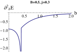
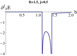
(a)	(b)

Figure 1: Second derivative of the ground energy with respect to $b$. The figures (a) and (b) are for $(B,j)=(0.5,0.3)$ and $(B,j)=(1.5,0.5)$, respectively. It is observed that the second derivative diverges at the QCPs $B=\sqrt{J^{2}+b^{2}}$ and $B=\sqrt{j^{2}+b^{2}}$.

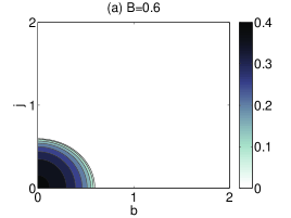
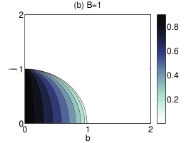
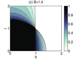
Figure 2: Magnetization at zero temperature. The figures (a), (b) and (c) show $B=0.6$, $B=1$ and $B=1.4$, respectively. The magnetization changes non-smoothly at the quantum critical points $B=\sqrt{J^{2}+b^{2}}$ and $B=\sqrt{j^{2}+b^{2}}$.

In this section, we investigate the properties of the ground state. Without the alternating coupling strength and the alternating magnetic field, the Hamiltonian is referred to as an XX model with a transverse magnetic field. It is well known that the XX model has a second order QPT at $B=J$ Takahashi . We investigate the ground state energy as a function of the alternating coupling strength and the alternating magnetic field, and see the QPTs induced by them.

We first define $Q$ as

$$Q=\{Q\in[0,\pi]|\Lambda^{-}_{q}<0\}.$$ (12)

For simplicity, we also introduce two functions,

$$\Theta(q) =\sqrt{J^{2}\cos^{2}q+b^{2}+j^{2}\sin^{2}q},$$ (13)

$$\Xi =\arccos\sqrt{\frac{B^{2}-b^{2}-j^{2}}{J^{2}-j^{2}}}.$$ (14)

By using the internal energy per site $u$ given by Eq. (6), the ground state energy per site is obtained by taking the limit such as

$$\epsilon_{g} =-\lim_{\beta\rightarrow\infty}\int_{0}^{\pi}\frac{dq}{2\pi}[\Lambda^{+}_{q}\tanh(\beta\Lambda^{+}_{q})+\Lambda^{-}_{q}\tanh(\beta\Lambda^{-}_{q})]$$

$$=-\int_{q\notin Q}\frac{dq}{2\pi}[\Lambda^{+}_{q}+\Lambda^{-}_{q}]-\int_{q\in Q}\frac{dq}{2\pi}[\Lambda^{+}_{q}-\Lambda^{-}_{q}]$$

$$=-B+\frac{1}{\pi}\int_{q\in Q}[B-\Theta(q)]dq.$$ (15)

In Appendix A, the region $Q$ is analytically obtained and exact expressions of the ground state energy are shown. In order to visualize the QPTs, the second derivative of the ground state in terms of $b$ for $(B,j)=(0.5,0.3)$ and $(B,j)=(1.5,0.5)$ is given in Fig. 1. It is observed that the derivative diverges at the points $B=\sqrt{J^{2}+b^{2}}$ and $B=\sqrt{j^{2}+b^{2}}$, both of which lead to second order QPTs.

The QPTs are observed more clearly by looking at the magnetic susceptibility at zero temperature. In Appendix A, the magnetization at zero temperature is explicitly calculated, which is a function of $\Xi$. Since the derivative of $\Xi$ by $B$ and $b$ includes a factor $1/\sqrt{B^{2}-b^{2}-j^{2}}\sqrt{-B^{2}+J^{2}+b^{2}}$, the derivative diverges at the points $B=\sqrt{J^{2}+b^{2}}$ and $B=\sqrt{j^{2}+b^{2}}$, which implies QPTs. To demonstrate this, we also plot the magnetization at zero temperature in Fig. 2. We can clearly see that the magnetization of the ground state changes non-smoothly at both QCPs.

We note that, when $j=b=0$ corresponding to the XX model with a transverse magnetic field, $B=\sqrt{J^{2}+b^{2}}$ reduces to the QCP of the XX model, $B=J$. On the other hand, QPTs at $B=\sqrt{j^{2}+b^{2}}$ do not appear in the XX model. Hence this QCP can be regarded as being induced by the staggered nature of the spin chain.

V Entanglement

We study the entanglement properties of the spin chain in three different ways. First we define the Meyer-Wallach measure and the concurrence and discuss how to calculate each for the staggered Hamiltonian. Next we consider how both entanglement measures behave at zero temperature, and then how a finite temperature affects the concurrence. Finally we consider a thermodynamic entanglement witness in an attempt to detect thermal entanglement which the measures miss such as multipartite entanglement.

V.1 Meyer-Wallach measure and Concurrence

First, we show how to calculate the Meyer-Wallach measure and the concurrence from the thermodynamic quantities calculated in Section II and correlation functions in Section III.

For a pure state $|\Phi\rangle$ of an $N$-spin system, the Meyer-Wallach measure is defined by

$$E_{\mathrm{MW}}(|\Phi\rangle)=2-\frac{2}{N}\sum_{i=1}^{N}{\rm Tr}\rho_{i}^{2},$$

where $\rho_{i}:={\rm Tr}_{\neg i}|\Phi\rangle\langle\Phi|$ is the reduced density matrix at the $i$-th spin  MW2002 ; B2003 . (The partial trace ${\rm Tr}_{\neg i}$ is taken over all degrees of freedom except the $i$-th spin.) The Meyer-Wallach measure takes values between $0$ and $1$. The minimum is achieved if and only if the state is separable while the maximum is given by states which are local unitary equivalent to the GHZ state.

We calculate the entanglement of the ground state found by the Meyer-Wallach measure. Since the Hamiltonian preserves the magnetization, i.e., $[H,\sum_{l}\sigma_{l}^{z}]=0$, the reduced density matrix of a spin at site $l$, $\rho_{l}$, has only diagonal elements such that $\rho_{l}={\rm diag}\{\frac{1+\langle\sigma_{l}^{z}\rangle_{g}}{2},\frac{1-\langle\sigma_{l}^{z}\rangle_{g}}{2}\}$ where $\langle\sigma_{l}^{z}\rangle_{g}:=\langle g|\sigma_{l}^{z}|g\rangle$ is the expectation value of $\sigma_{l}^{z}$ by the ground state $|g\rangle$. By substituting this and using the fact that the Hamiltonian is semi-translationally invariant, the Meyer-Wallach measure of the ground state is obtained as

$$E_{\mathrm{MW}}(|g\rangle)=1-\frac{1}{2}(\langle\sigma_{even}^{z}\rangle_{g}^{2}+\langle\sigma_{odd}^{z}\rangle_{g}^{2}).$$ (16)

where $\langle\sigma_{even}^{z}\rangle_{g}=\langle g|\sigma_{2l}^{z}|g\rangle$ and $\langle\sigma_{odd}^{z}\rangle_{g}=\langle g|\sigma_{2l+1}^{z}|g\rangle$ for any $l$. The $\langle\sigma_{even}^{z}\rangle$ and $\langle\sigma_{odd}^{z}\rangle$ are obtained from the magnetization $m$ given by Eq. (7) and $m_{s}$ given by Eq. (8) such as

$$\langle\sigma_{even}^{z}\rangle_{g} =\lim_{\beta\rightarrow\infty}[m+m_{s}],$$ (17)

$$\langle\sigma_{odd}^{z}\rangle_{g} =\lim_{\beta\rightarrow\infty}[m-m_{s}].$$ (18)

The exact expressions of the ground state energy, the magnetization at zero temperature and the Meyer-Wallach measure are given in Appendix A. Note that the Meyer-Wallach measure is a measure of entanglement only for pure states, and thus is meaningful for investigation of entanglement in the ground state but not that of thermal states.

The concurrence, ${\mathcal{C}}$, between two spins OConnor is an entanglement measure for both pure and mixed states, and can therefore be used at finite temperatures. It is given by

$${\mathcal{C}}(\rho)=\max\{0,\lambda_{1}-\lambda_{2}-\lambda_{3}-\lambda_{4}\},$$ (19)

where the $\lambda_{i}$s are the square roots of the eigenvalues of the matrix $\rho\tilde{\rho}$ with $\tilde{\rho}=(\sigma^{y}\otimes\sigma^{y})\rho^{*}(\sigma^{y}\otimes\sigma^{y})$, and satisfy $\lambda_{1}\geq\lambda_{2}\geq\lambda_{3}\geq\lambda_{4}$. Again using $[H,\sum_{l}\sigma_{l}^{z}]=0$, the concurrence between two spins at sites $l$ and $l+R$ is ${\mathcal{C}}(\rho_{l,l+R})=2\max\{0,|z|-\sqrt{vy}\}$ where $z=\frac{1}{4}\langle\sigma_{l}^{x}\sigma_{l+R}^{x}+\sigma_{l}^{y}\sigma_{l+R}^{y}\rangle$, and $vy=\frac{1}{16}[(1+\langle\sigma_{l}^{z}\sigma_{l+R}^{z}\rangle)^{2}-(\langle\sigma_{l}^{z}\rangle+\langle\sigma_{l+R}^{z}\rangle)^{2}]$. Due to the semi-translational invariance of the Hamiltonian, the concurrence is the same for all odd sites and for all even sites. The concurrence is zero if and only if the state of the two spins is separable, and is one when they are maximally entangled. Although we could calculate the concurrence for any $R$, we concentrate on the nearest neighbour, ${\mathcal{C}}_{1}$ with $R=1$, and the next nearest neighbour, ${\mathcal{C}}_{2}$ with $R=2$, concurrence since for large $R$ the concurrence is infinitesimal. Using $\langle\sigma_{l}^{z}\sigma_{l+R}^{z}\rangle=\langle\sigma_{l}^{z}\rangle\langle\sigma_{l+R}^{z}\rangle-G_{l,R}^{2}$, the nearest neighbour concurrence is

$${\mathcal{C}}_{1}=\max\left\{0,\left|G_{l,1}\right|-\frac{1}{2}\sqrt{\left(1+\langle\sigma_{l}^{z}\sigma_{l+1}^{z}\rangle\right)^{2}-\left(2\langle\sigma^{z}\rangle^{0}\right)^{2}}\right\},$$ (20)

and the next nearest neighbour concurrence is

$${\mathcal{C}}_{2} = \max\bigg{\{}0,\left|G_{l,1}G_{l+1,1}-G_{l,2}\langle\sigma_{l+1}^{z}\rangle\right|\bigg{.}$$

$$- \left.\frac{1}{2}\sqrt{\left(1+\langle\sigma_{l}^{z}\sigma_{l+2}^{z}\rangle\right)^{2}-\left(2\langle\sigma_{l}^{z}\rangle\right)^{2}}\right\},$$

remembering that $G_{R}$ is different for odd and for even values of $R$.

When $J=j$, the total coupling strength between nearest neighbour sites for odd $l$ is zero, while for even $l$, it is $2J$. Thus, at any temperature, there is no entanglement between nearest neighbours for odd sites, and at zero temperature (and magnetic fields), the chain consists of $N/2$ maximally entangled singlet states. This is an example of dimerisation. As a consequence of this, there is also no concurrence at $J=j$ for both odd and even sites for any $R>1$.

We note that unlike the Meyer-Wallach measure, the concurrence is not directly related to the total amount of entanglement contained in a pure state. Hence, there is no guarantee that the Meyer-Wallach measure and the concurrence will behave similarly. For instance, for the GHZ state, the Meyer-Wallach measure is one but the concurrence between any two spins is zero.

V.2 Zero temperature

In this section, we study entanglement at zero temperature using the Meyer-Wallach measure and the concurrence as defined above. Figs. 3 and 5 show the Meyer-Wallach measure, Figs. 4 and 6 the nearest neighbour (NN) concurrence for both odd and even sites, and Fig. 7 the next nearest neighbour (NNN) concurrence.

V.2.1 Quantum phase transitions

We first discuss the Meyer-Wallach measure of the ground state. See Appendix A for the detailed calculation. In Figs. 3 and 5, it is observed that the Meyer-Wallach measure changes non-smoothly at the QCPs.

Conversely, considering the plots for concurrence at zero temperature, the quantum phase transitions present in the staggered model are not always evident. In particular, when plotting $B$ against $b$ for odd sites in Fig. 4, only the curve $B=\sqrt{J^{2}+b^{2}}$ can be seen in (b), while only $B=\sqrt{j^{2}+b^{2}}$ can be seen in (c). However, changes in the concurrence can be observed at both QCPs for even $l$ in the same figure, and for both odd and even sites in Fig. 6 where we plot $B$ against $j$.

These results are consistent with the results in Ref. WSL2004 , where it is shown that entanglement of the ground state behaves singularly around QCPs in general.

V.2.2 Effects of $j$ and $b$ on entanglement

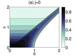
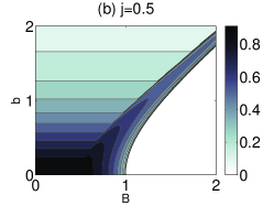
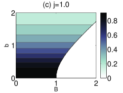
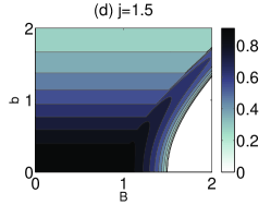
Figure 3: The Meyer-Wallach measure as a function of $B$ and $b$.

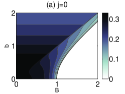
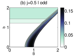
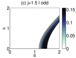
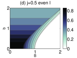
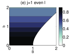
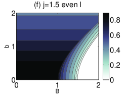
Figure 4: The nearest neighbour concurrence as a function of $B$ and $b$ as $T\rightarrow 0$. When $j=0$, (a), the concurrence for odd and for even sites is identical.

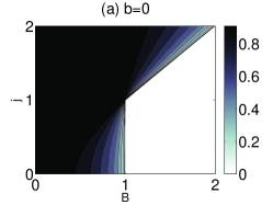
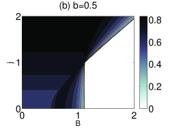
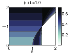
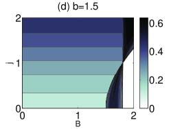
Figure 5: The Meyer-Wallach measure as a function of $B$ and $j$.

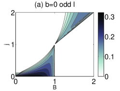
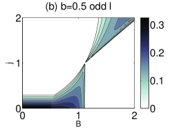
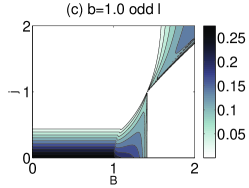
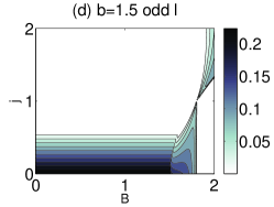
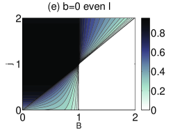
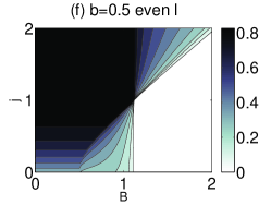
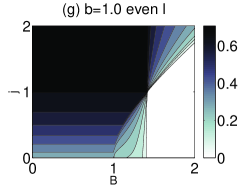
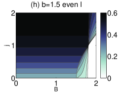
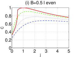
Figure 6: The nearest neighbour concurrence as a function of $B$ and $j$ as $T\rightarrow 0$. (i) plots the concurrence against $j$ for $l$ even, $B=0.5$ to show that the concurrence decreases for high enough $j$ for $b=0$ (solid red line), $b=0.5$ (dashed green line), $b=1$ (dotted purple line) and $b=1.5$ (dot-dashed blue line).

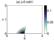
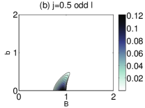
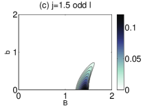
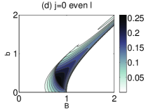
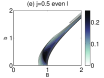
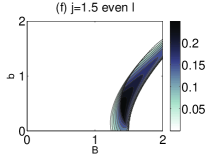
Figure 7: Next nearest neighbour concurrence as $T\rightarrow 0$. Concurrence is zero when $j=1$ as discussed in the text.

Next, we discuss the effects of $b$ and $j$ on the Meyer-Wallach measure and the concurrence.

First, we consider the effect of $b$ on the entanglement, shown in Figs. 3 and 4. How the concurrence behaves in the presence of the alternating fields is highly dependent on whether the site is odd or even. In general, due to the larger coupling from an even site to an odd site, both nearest (NN) and next nearest neighbour (NNN) concurrence is higher, with the opposite being true from an odd to an even site. Entanglement for the Meyer-Wallach measure and odd site NN concurrence remains large only when $B$ is between the two QPTs, i.e. $\sqrt{j^{2}+b^{2}}<B<\sqrt{J^{2}+b^{2}}$ when $j<J$ or $\sqrt{J^{2}+b^{2}}<B<\sqrt{j^{2}+b^{2}}$ when $J<j$. For both measures, the maximum entanglement is at $B\sim b$ for large magnetic fields. These results are understandable from the fact that a large magnetic field aligns spins in the same direction leading to a separable state. When $b$ and $B$ are large, entanglement can be large only for $B\sim b$ since the magnetic field on odd sites is canceled in such cases.

The even site NN concurrence does not follow this pattern, and instead a larger amount of entanglement tends to be present when $B<\sqrt{j^{2}+b^{2}}$ for $j<J$ or when $B<\sqrt{J^{2}+b^{2}}$ for $J<j$.

On the other hand, the Meyer-Wallach measure and the concurrence vary differently with the alternating coupling constant $j$ as shown in Figs. 5 and 6 where the entanglement is plotted as a function of $j$. The Meyer-Wallach measure is an increasing function with $j$ except in the vicinity of the QCPs while the concurrence is in general a decreasing function of $j$. Fig. 6 (i) shows that for each $b$, there is a non-zero value of $j$ for which the concurrence is the maximum possible. Since the Meyer-Wallach measure is a measure of the entanglement shared in the whole spin chain and the concurrence measures the entanglement between two spins, we can conclude from these results that as the alternating coupling constant $j$ increases, the amount of entanglement shared amongst all spins increases. Such global entanglement is not locally detected, in the sense that the entanglement of the reduced two spin state is small.

The concurrence is closely related to the entanglement of formation. In Fig. 6, for odd sites, when $B>\sqrt{J^{2}+b^{2}}$, increasing $j$ can increase concurrence, and for even sites, when $B<\sqrt{j^{2}+b^{2}}$, increasing $j$ increases the concurrence until a maximal value is reached, after which the concurrence decreases again. Thus a low but non-zero value of $j$ can be beneficial to the extraction of maximally entangled state.

Another interesting feature common to both the Meyer-Wallach measure and the concurrence, demonstrated in Figs. 3- 6, is that below the region of the QCPs, the entanglement is constant as $B$ varies. That is, the magnetic field $B$ is not a dominant parameter for entanglement below the QCPs. The QPTs are often intuitively understood as occurring due to the balance between the strength of the coupling constants and that of the magnetic fields. As such, the dominant parameters of this system are the coupling constants (the magnetic fields) below (above) the QCPs in general. Our results support this intuition from the viewpoint of entanglement in the sense that the magnetic field $B$ does not change the entanglement below the QCPs. On the other hand, the entanglement is sensitive to the change of the alternating magnetic field $b$ even below the QCPs, which demonstrates the difference between $B$ and $b$.

Finally, the NNN concurrence is reduced compared to NN concurrence as expected, but remains reasonably high, especially for even sites where a non-zero value of $b$ increases the entanglement. Further, increasing $b$ allows a spin chain with larger values of $B$ to be entangled.

V.3 Finite temperature

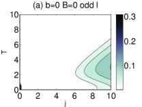
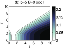
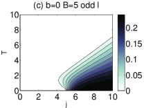
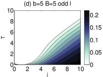
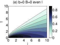
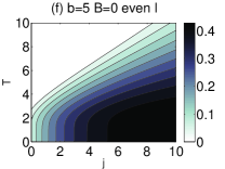
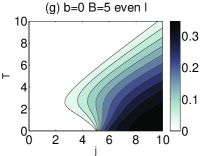
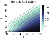
Figure 8: Nearest neighbour concurrence for odd and even sites.

We next investigate the entanglement properties of the thermal states of the Hamiltonian using the concurrence.

Fig. 8 plots the nearest neighbour concurrence for both odd and even sites for varying temperature and alternating coupling strength, $j$. The figures show that increasing $j$ allows the spin chain to be entangled at higher temperatures, and that increasing both $b$ and $B$ can enlarge the region of entanglement. That is, the spin chain is entangled for more values of $T$ and $j$ for higher $b$ and $B$. This is true for even as well as odd sites. Next nearest neighbour concurrence can be seen in Fig. 9 where we again see that increasing the magnetic fields can be beneficial to entanglement. As discussed previously, there is no entanglement at $j=1$ for odd sites at any temperature.

Increasing temperature has the effect of mixing energy levels, something which has the ability to either increase or decrease entanglement, though a high enough temperature will destroy entanglement. Increasing the alternating coupling strength counteracts this to some extent, though a high enough temperature will still destroy the concurrence.

We note that increasing $b$ allows larger values of concurrence at higher temperatures at lower, more accessible values of $j$ as demonstrated in Fig. 8 (b) and (f). Thus it is the combination of alternating fields $b$ and $j$ that allow the spin chain to be entangled at higher temperatures. Increasing $B$ has a similar effect, though to a lesser extent.

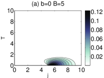
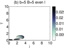
Figure 9: Next nearest neighbour concurrence. When $b=0$ and $B=5$, (a), the plot for odd and even sites is identical. No next nearest neighbour concurrence is found for the other values of $B$ and $b$ shown for nearest neighbour concurrence.

V.4 An entanglement witness

In order to detect rather than measure entanglement in this system, we use an entanglement witness based on the expectation value of the Hamiltonian:

$$\frac{4|U+BM+bM_{s}|}{N(|J-j|+|J+j|)}\leq 1,$$ (22)

where $U$ is the internal energy (Eq. 6) $M$ is the magnetisation (Eq. 7) and $M_{s}$ is the staggered magnetisation (Eq. 8). The bound is found similarly to the usual method ent_wit ; vlat . Rearranging the expectation value of the Hamiltonian gives $2|U+BM+bM_{s}|=|J\sum_{l}\langle\sigma_{l}^{x}\sigma_{l+1}^{x}+\sigma_{l}^{y}\sigma_{l+1}^{y}\rangle+j\sum_{l}e^{i\pi l}\langle\sigma_{l}^{x}\sigma_{l+1}^{x}+\sigma_{l}^{y}\sigma_{l+1}^{y}\rangle|$. The absolute sign allows us to write $4|U+BM+bM_{s}|/N\leq|(J-j)||\langle\sigma_{l}^{x}\sigma_{l+1}^{x}+\sigma_{l}^{y}\sigma_{l+1}^{y}\rangle|_{l,odd}+|J+j||\langle\sigma_{l}^{x}\sigma_{l+1}^{x}+\sigma_{l}^{y}\sigma_{l+1}^{y}\rangle|_{l,even}$. Next, the bound for both the odd and even $l$ for pure product states can be found using the Cauchy-Schwarz inequality, and the definition of the density matrix giving $|\langle\sigma_{l}^{x}\sigma_{l+1}^{x}+\sigma_{l}^{y}\sigma_{l+1}^{y}\rangle|\leq 1$. Due to the convexity of the set of separable states, this bound is also true for all separable states while an entangled state can violate this bound.

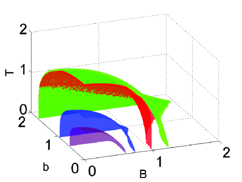
Figure 10: We witness the entanglement at different values of the alternating coupling strength, $j$ for $j=0$ purple, $j=0.5$ blue, $j=1$ red, $j=1.5$ green, from inside to out.

Fig. 10 demonstrates that increasing the alternating coupling strength increases the region of entanglement detected by the witness. That is, at larger $j$, entanglement is detected for higher values of $B$, $b$ and $T$ than is possible at smaller $j$. This trend persists even at very high values of $j$. In addition, the alternating magnetic field increases the maximum values of $B$ for which entanglement is detected. However, overall, increasing $B$, $b$ or $T$ enough (except at $B\sim b$ as discussed in Section V.2) will destroy entanglement either by causing the spins to align with the magnetic field, or via the mixing of energy levels as the temperature is raised.

The entanglement witness generally complements the results of the entanglement measures, and allows for the possibility of detecting multipartite entanglement that cannot be measured by them. However, for our Hamiltonian, comparing Fig. 10 to Figs. 8 and 9, it can be seen that this witness does not detect any extra entangled regions compared to the concurrence.

VI Concluding Remarks

We have found that the introduction of an alternating coupling strength and alternating magnetic field into the usual $XX$ spin chain in a uniform magnetic field can, for certain values of the parameters, increase both the amount and region of entanglement quantified by either the Meyer-Wallach measure or the concurrence. This is the case for both zero and finite temperatures. We have demonstrated that two quantum phase transitions exist in this system, signs of which are evident in both entanglement measures. In addition, we have calculated an entanglement witness which detects entanglement within a region which agrees with the measures of entanglement we consider.

It would be interesting to calculate the finite temperature effects of the quantum phase transitions in this model. Determining the effect on entanglement of increasing the period of the staggered parameters would also be an interesting extension to this work. For example, by varying the magnetic field and coupling strength over three sites $l$, $l+1$ and $l+2$ rather than the two considered here. However, this may not be possible to do analytically.

Appendix A Calculations of quantities at zero temperature

Here, we give exact expressions of the ground energy, the magnetization at zero temperature and the Meyer-Wallach measure of the ground state. For simplicity, we define regions such as

$$\mathcal{B}_{1} :=[0,\sqrt{J^{2}+b^{2}}),$$ (23)

$$\mathcal{B}_{2} :=[\sqrt{J^{2}+b^{2}},\sqrt{j^{2}+b^{2}}),$$ (24)

$$\mathcal{B}_{3} :=[\sqrt{j^{2}+b^{2}},\infty),$$ (25)

$$\mathcal{B}_{3}^{\prime} :=[\sqrt{J^{2}+b^{2}},\infty)$$ (26)

A.1 Ground energy

First, we show the exact expressions of the ground energy $\epsilon_{g}$ given by Eq. (15).

$j<J$

In this case, $Q$ is given by

$$Q=(0,\Xi)\cup(\pi-\Xi,\pi).$$ (27)

It is straightforward to calculate the ground energy;

$$\epsilon_{g}=\begin{cases}(\frac{2}{\pi}\Xi-1)B-\frac{2}{\pi}\int_{0}^{\Xi}\Theta(q)dq,&\text{for }B\in\mathcal{B}_{1}\\ -B,&\text{for }B\in\mathcal{B}_{3}^{\prime}.\end{cases}$$ (28)

$j=J$

Since $\Lambda_{q}^{-}=2B-2\sqrt{J^{2}+b^{2}}$, the ground energy is obtained as

$$\epsilon_{g}=\begin{cases}-\sqrt{J^{2}+b^{2}},&\text{for }B\in\mathcal{B}_{1}\\ -B,&\text{for }B\in\mathcal{B}_{3}^{\prime}.\end{cases}$$ (29)

$j>J$

In this case, $Q$ is given by

$$Q=(\Xi,\pi-\Xi).$$ (30)

Then, the ground energy is calculated as

$$\epsilon_{g}=\begin{cases}-\frac{2}{\pi}\int_{0}^{\pi/2}\Theta(q)dq,&\text{for }B\in\mathcal{B}_{1}\\ -\frac{2}{\pi}\Xi B-\frac{2}{\pi}\int_{\Xi}^{\pi/2}\Theta(q)dq,&\text{for }B\in\mathcal{B}_{2}\\ -B,&\text{for }B\in\mathcal{B}_{3}.\end{cases}$$ (31)

A.2 Magnetization at zero-temperature

We show the magnetization at zero temperature per site $m_{g}$. The magnetization $m_{g}$ is directly obtained from Eq. (7) such as

$$m_{g} =\lim_{\beta\rightarrow\infty}\int_{0}^{\pi}\frac{dq}{2\pi}[\tanh(\beta\Lambda^{+})+\tanh(\beta\Lambda^{-})]$$ (32)

$$=\int_{q\notin Q}\frac{dq}{\pi}.$$ (33)

By substituting $Q$, the magnetization is obtained as follows; for $j<J$

$$m_{g}=\begin{cases}1-\frac{2}{\pi}\Xi,&\text{for }B\in\mathcal{B}_{1}\\ 1,&\text{for }B\in\mathcal{B}_{3}^{\prime},\end{cases}$$ (34)

for $j=J$,

$$m_{g}=\begin{cases}0,&\text{for }B\in\mathcal{B}_{1}\\ 1,&\text{for }B\in\mathcal{B}_{3}^{\prime},\end{cases}$$ (35)

and, for $j>J$,

$$m_{g}=\begin{cases}0,&\text{for }B\in\mathcal{B}_{1}\\ \frac{2}{\pi}\Xi,&\text{for }B\in\mathcal{B}_{2}\\ 1,&\text{for }B\in\mathcal{B}_{3}.\end{cases}$$ (36)

A.3 Meyer-Wallach measure of the ground state

Here, we give the exact expressions of the Meyer-Wallach measure of the ground state, $E_{\rm MW}$, given by Eq. (16). For $j<J$,

$$E_{\rm MW}=\begin{cases}\frac{4}{\pi}\Xi(1-\frac{\Xi}{\pi})-(\frac{2b}{\pi}\int_{0}^{\Xi}\frac{1}{\Theta(q)}dq)^{2}&\text{for }B\in\mathcal{B}_{1}\\ 0,&\text{for }B\in\mathcal{B}_{3}^{\prime}.\end{cases}$$ (37)

For $j=J$,

$$E_{\rm MW}=\begin{cases}\frac{J^{2}}{J^{2}+b^{2}}&\text{for }B\in\mathcal{B}_{1}\\ 0&\text{for }B\in\mathcal{B}_{3}^{\prime}.\end{cases}$$ (38)

Finally, for $j>J$,

$$E_{\rm MW}=\begin{cases}1-(\frac{2b}{\pi}\int_{0}^{\pi/2}\frac{1}{\Theta(q)}dq)^{2}&\text{for }B\in\mathcal{B}_{1}\\ 1-\frac{4\Xi^{2}}{\pi^{2}}-(\frac{2b}{\pi}\int_{\Xi}^{\pi/2}\frac{1}{\Theta(q)}dq)^{2}&\text{for }B\in\mathcal{B}_{2}\\ 0&\text{for }B\in\mathcal{B}_{3}.\end{cases}$$ (39)

References

- (1) L. Amico, R. Fazio, A. Osterloh and V. Vedral, Rev. Mod. Phys. 80, 517 (2008)
- (2) D. P. Divincenzo et al. Nature 408, 339 (2000)
- (3) S. Bose, Phys. Rev. Lett. 91, 207901 (2003)
- (4) C. H. Bennett, H. J. Bernstein, S. Popescu, and B. Schumacher, Phys. Rev. A 53, 2046 (1996).
- (5) D. A. Meyer and N. R. Wallach, J. Math. Phys. 43 4273 (2002).
- (6) K. M. O’Connor and W. K. Wootters, Phys. Rev. A 63, 052302 (2001)
- (7) G. Toth, Phys. Rev. A 71, 010301(R) (2005)
- (8) Č. Brukner and V. Vedral, Arxiv: quant-ph/0406040
- (9) S. Sachdev, Quantum Phase Transitions Cambridge University Press (1999).
- (10) L. A. Wu, M. S. Sarandy, and D. A. Lidar, Phys. Rev. Lett. 93, 250404 (2004).
- (11) M. Oshikawa and I. Affleck, Phys. Rev. Lett. 79, 2883 (1997).
- (12) D. B. Abraham, J. Chem. Phys. 51, 3795 (1969)
- (13) P. Pincus, Solid State Communications. 9, 1971 (1971)
- (14) J. Hide, W. Son, I. Lawrie and V. Vedral, Phys. Rev. A 76, 022319 (2007)
- (15) R. H. Crooks and D. V. Khveshchenko, Phys. Rev. A 77, 062305 (2008)
- (16) S. I. Doronin, A. N. Pyrkov, and E. B. Felman, JETP 105, 953 (2007)
- (17) J. H. H. Perk, H. W. Capel, M. J. Zuilhof and Th. J. Siskens, Physica A 81, 319 (1975)
- (18) E. Barouch and B. M. McCoy, Phys. Rev. A 3, 786 (1971)
- (19) J. H. H. Perk and H. W. Capel, Physica A 92 163 (1978)
- (20) J. H. H. Perk, H. W. Capel and Th. J. Siskens, Physica A 89 304 (1977)
- (21) M. Takahashi, Thermodynamics of One-Dimensional Solvable Models, Cambridge University Press (1999).
- (22) G. K. Brennen, Quantum Information and Computation, vol. 3 (6), 619-626 (2003).