Bulk viscosity in heavy ion collision

Abstract

The effect of a temperature dependent bulk viscosity to entropy density ratio ($\zeta/s$) along with a constant shear viscosity to entropy density ratio ($\eta/s$) on the space time evolution of the fluid produced in high energy heavy ion collisions have been studied in a relativistic viscous hydrodynamics model. The boost invariant Israel-Stewart theory of causal relativistic viscous hydrodynamics is used to simulate the evolution of the fluid in 2 spatial and 1 temporal dimension. The dissipative correction to the freezeout distribution for bulk viscosity is calculated using Grad’s fourteen moment method. From our simulation we show that the method is applicable only for $\zeta/s<0.004$.

I Introduction

Recent experiments in high energy nuclear collisions at relativistic heavy ion collider (RHIC) confirms the existence of a new state of matter known as Quark Gluon Plasma (QGP) journal-1 . The production of QGP in heavy ion collision and its subsequent collective evolution provide us the unique opportunity to study the transport properties of this most fundamental form of matter. Relativistic viscous hydrodynamics simulations of observables like elliptic flow ($v_{2}$) and transverse momentum ($p_{T}$) spectra have been compared to experimental data to extract the QGP $\eta/s$. Most studies show that the estimated value of $\eta/s$ lies between $1-4\times(1/4\pi)$. However to correctly extract the $\eta/s$ of the QGP fluid, it is important to know the effect of finite bulk viscosity on the fluid evolution. Theoretical calculations based on pQCD journal-2 and lattice QCD journal-3 shows that the bulk viscosity is non-zero for the temperature range applicable in the heavy ion collision. In this work we use a temperature dependent form of $\zeta/s$ to study the effect of bulk viscosity in fluid evolution. The dissipative correction to the freezeout distribution function bulk viscosity has also been considered using Grad’s 14 moment method.

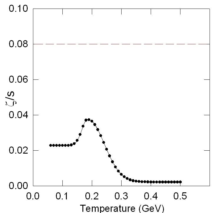
Figure 1: (Color online) $\zeta/s$ as a function of temperature. Red dashed line is the $\eta/s=1/4\pi$.

II Viscous hydrodynamic model

The space time evolution of the fluid was simulated by simultaneously solving the energy momentum conservation equation $\partial_{\mu}T^{\mu\nu}=0$, along with the relaxation equation for shear and bulk stress. Here $T^{\mu\nu}=(\epsilon+p+\Pi)u^{\mu}u^{\nu}-(p+\Pi)g^{\mu\nu}+\pi^{\mu\nu}$ is the energy momentum tensor and $\epsilon,p$ are energy density, pressure of the fluid,$g^{\mu\nu}$ is the metric tensor; $\Pi$ and $\pi^{\mu\nu}$ are bulk and shear stress tensor respectively. According to the Israel-Stewart theory of causal viscous hydrodynamics journal-4 , the shear and bulk viscosity obey the following relaxation equations $D\pi^{\mu\nu}=\frac{1}{\tau_{\pi}}[2\eta\nabla^{<^{\mu}u^{\nu}>}-\pi^{\mu\nu}]-\left(u^{\mu}\pi^{\nu\lambda}+u^{\nu}\pi^{\mu\lambda}\right)Du_{\lambda}$; and $D\Pi=-\frac{1}{\tau_{\Pi}}[\Pi+\zeta\nabla_{\mu}u^{\mu}+\frac{1}{2}\zeta T\Pi\partial_{\mu}(\frac{\tau_{\Pi}u^{\mu}}{\zeta T})]$. Here D is the convective derivative,$\tau_{\pi}$ and $\tau_{\Pi}$ are the relaxation time for shear and bulk stresses respectively. We assume that the fluid achieve near local thermalization at proper time 0.6 fm. Initial transverse velocity ($v_{T}$) is assumed to be zero. The initial energy density profile in transverse plane is calculated from a two component Glauber model with a central energy density $\epsilon_{0}=30GeV/fm^{3}$. Initial value of $\pi^{\mu\nu}$ and $\Pi$ was set to their corresponding Navier-Stokes estimate. We assume the fluid freezes out when an element of it cools down below a constant temperature $T_{fo}=130$ MeV. The freezeout procedure was carried out by using Cooper-Frey algorithm. In the present study, we have used an equation of state (EoS) where the Wuppertal-Budapest lattice calculation journal-3 for the deconfined phase is smoothly joined at crossover temperature 174 MeV, with hadronic resonance gas EoS comprising all the resonances below mass $m_{res}$=2.5 GeV. $\zeta/s$ and $\eta/s$ are inputs to viscous hydrodynamics simulation. Figure 1 shows the $\zeta/s$(T), where $\zeta/s$ in the QGP phase is obtained by using pQCD formula $\zeta/s=15\frac{\eta}{s}(T)(1/3-c^{2}_{s}(T))^{2}$, the squared speed of sound $c^{2}_{s}$ was calculated from lattice data journal-5 . In the hadronic phase $\zeta/s$ is parametrized from journal-6 . The red dashed line in figure 1 is $\eta/s$.

III Results and discussion

We first discuss the change in pion $p_{T}$ spectra and $v_{2}$ due to bulk and shear viscosity in the fluid evolution only. In the left panel of figure 2 temporal evolution of spatially averaged transverse velocity $\left\langle\left\langle v_{T}\right\rangle\right\rangle=\frac{\left\langle\left\langle\gamma\sqrt{v^{2}_{x}+v^{2}_{y}}~{}\right\rangle\right\rangle}{\left\langle\left\langle\gamma\right\rangle\right\rangle}$ is shown for ideal, shear and bulk viscous fluid. Here the angular bracket denotes space average and $\gamma=\frac{1}{\sqrt{1-v^{2}}}$. Because of the reduced pressure in bulk viscous evolution, $\left\langle\left\langle v_{T}\right\rangle\right\rangle$ is reduced in comparison to ideal fluid evolution. Whereas shear viscosity increase the pressure in the transverse direction, as a result the $\left\langle\left\langle v_{T}\right\rangle\right\rangle$ is larger compared to ideal fluid. The effect of the changed fluid velocity in viscous evolution is reflected in the slope of the $p_{T}$ spectra of $\pi^{-}$ shown in the right panel of figure 2. The relative change in the $\pi^{-}$ invariant yield $(\delta N/N_{ideal},\delta N=N_{bulk}-N_{ideal})$ due to the bulk viscosity in comparison to ideal fluid is shown in the inset of right plot of figure 2. The relative correction is within $\sim 10\%$.

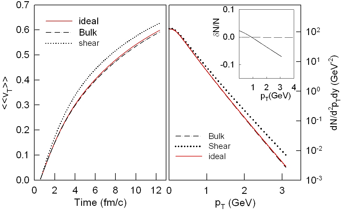
Figure 2: (Color online) The left plot shows the temporal evolution of fluid transverse velocity for ideal (red),bulk (dashed dot) and shear viscous (dotted) evolution. The right plot is the $\pi^{-}$ invariant yield as a function of $p_{T}$ for ideal (red) ,bulk dashed dot and shear viscous (dotted) evolution. The inset figure shows the relative correction to invariant yield due to the bulk viscosity in comparison to ideal fluid.

The temporal evolution of momentum space anisotropy $\epsilon_{p}=\frac{\int dxdy(T^{xx}-T^{yy})}{\int dxdy(T^{xx}+T^{yy})}$ is shown in the left panel of figure 3. Viscosity tries to diminish any velocity gradient present in the fluid, as a result of that $\epsilon_{p}$ is smaller for both shear and bulk viscous evolution compared to ideal fluid. In a hydrodynamic model $v_{2}$ is proportional to $\epsilon_{p}$ hence a reduction in $\epsilon_{p}$ will result in a reduced $v_{2}$. Elliptic flow of $\pi^{-}$ as a function of $p_{T}$ is shown for ideal, shear and bulk viscous evolution in the right plot of figure 3. The inset shows the relative correction to $v_{2}$ due to bulk viscosity. The relative correction to $v_{2}$ is within $\sim 3\%$.

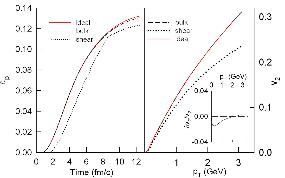
Figure 3: (Color online) The left plot is the temporal evolution of momentum anisotropy of the fluid for ideal(red),bulk(dashed dot) and shear viscous(dotted) evolution. Right plot is the corresponding elliptic flow ($v_{2}$) of $\pi^{-}$. The inset plot shows the relative change in $v_{2}$ due to bulk viscosity compared to ideal fluid.

We have employed Grad’s fourteen-moment method for calculating the dissipative correction to the freezeout distribution function as described in journal-7 . The details of the implementation of this method to our viscous code ”‘AZHYDRO-KOLKATA”’ can be found in journal-8 ; journal-9 . The top left panel of figure 4 shows the $p_{T}$ spectra of pions for ideal(black solid line) and for four different values of $\zeta/s$. The corresponding relative correction to the $p_{T}$ spectra is shown in the bottom left panel. The $v_{2}$ of pion and the relative correction is shown in the right panel of figure 4. Freeze-out correction in Grad’s moment method is obtained under the assumption that the non-equilibrium correction to the distribution function is small than the equilibrium distribution function. It is then implied that the relative correction $\delta N/N_{eq}$ is small for Grad’s method to be applicable. The shaded band in the bottom left panel corresponds to the relative correction of 50%. If we consider here a correction of magnitude greater than 50% indicates the breakdown of the the freezeout correction procedure then our study shows that the Grad’s method will be applicable if the $\zeta/s$ has value less than 0.01 times the present form considered here.

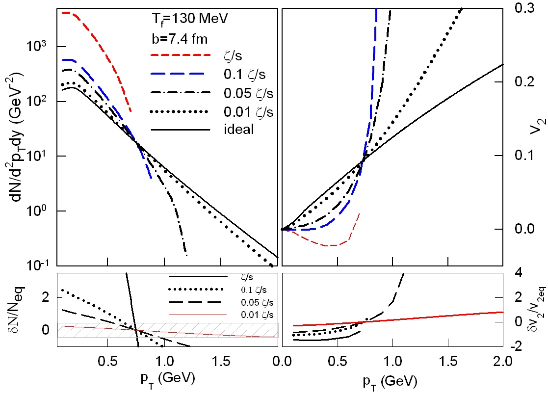
Figure 4: (Color online) The invariant yield of $\pi^{-}$ as a function of $p_{T}$ for ideal and bulk viscous evolution with four different $\zeta/s$ values are shown in the upper left plot. The lower left plot shows the relative correction to the $\pi^{-}$ yield as a function of $p_{T}$ for four different $\zeta/s$. See text for details. The right side plot is same as the left but for $v_{2}$.

References

- (1) J. Adams et al. [STAR Collaboration],Nucl. Phys. A 757, 102 (2005).
- (2) S. Weinberg,Astrophys. J. 168, 175 (1971).
- (3) H. B. Meyer,Phys. Rev. Lett. 100, 162001 (2008).
- (4) W. Israel,Annals of Physics 100,310-331 (1976).
- (5) S. Borsanyi et al.,JHEP 1011, 077 (2010).
- (6) J. Noronha-Hostler, J. Noronha and C. Greiner,Phys. Rev. Lett. 103, 172302 (2009).
- (7) A. Monnai and T. Hirano,Phys. Rev. C 80, 054906 (2009).
- (8) V. Roy, A. K. Chaudhuri, submitted to Phys. Rev. C.
- (9) A. K. Chaudhuri,arXiv:0801.3180 [nucl-th].