Dark Matter as an active gravitational agent in cloud complexes

Abstract

We study the effect that the dark matter background (DMB) has on the gravitational energy content and, in general, on the star formation efficiency of a molecular cloud (MC). We first analyze the effect that a dark matter halo, described by the Navarro et al. (1996) density profile, has on the energy budget of a spherical, homogeneous, cloud located at different distances from the halo center. We found that MCs located in the innermost regions of a massive galaxy can feel a contraction force greater than their self-gravity due to the incorporation of the potential of the galaxy’s dark matter halo. We also calculated analytically the gravitational perturbation that a MC produces over a uniform DMB (uniform at the scales of a MC) and how this perturbation will affect the evolution of the MC itself. The study shows that the star formation in a MC will be considerably enhanced if the cloud is located in a dense and low velocity dark matter environment. We confirm our results by measuring the star formation efficiency in numerical simulations of the formation and evolution of MCs within different DMBs. Our study indicates that there are situations where the dark matter’s gravitational contribution to the evolution of the molecular clouds should not be neglected.

1. INTRODUCTION

A great effort from the astronomical community is currently directed towards the detailed understanding of star formation, in particular to the precise mechanisms involved in the conversion of some part of a molecular cloud’s mass into stars. The evolution of molecular clouds (MCs) and the formation of stars within them are thought to be regulated by actors as diverse as gravity, large-scale flows, turbulence, magnetic fields, and stellar feedback, among others (see reviews by Shu et al., 1987; Vázquez-Semadeni, 2010).

While evaluating the dynamical state of a molecular cloud due to all relevant forces acting on it, the Virial Theorem is frequently invoked to define an equilibrium condition by equaling the gravitational energy $W$ of the cloud to twice its kinetic energy $K$:

$$2K=-W.$$ (1)

Traditionally, this relationship has been interpreted in terms of clouds being in a state of quasi-equilibrium and long-lived entities, and deviations from this condition are assumed to mean that the cloud is collapsing or expanding, depending on which term is dominant (e.g., Myers & Goodman, 1988a, b; McKee & Zweibel, 1992). However, it has been demonstrated that a cloud fullfiling the so-called equilibrium condition will not necessarily remain dynamically stable (Ballesteros-Paredes, 2006). In fact, numerical simulations show that clouds collapsing in a chaotic and hierarchical way will develop such a relationship (e.g., Vázquez-Semadeni et al., 2007; Ballesteros-Paredes et al., 2011a, b).

Furthermore, when calculating the Virial Theorem for MCs, it is a common practice to consider that the gravitational term is the gravitational energy, assuming that the cloud is, in practice, an isolated entity. However, different recent works have showed that the media surrounding the dense structures can importantly alter the evolution of such entities (e.g., Burkert & Hartmann, 2004; Gómez et al., 2007; Vázquez-Semadeni et al., 2007; Heitsch & Hartmann, 2008; Ballesteros-Paredes et al., 2009b, a). In these works, the influence of barionic matter outside the region of interest is studied.

On an apparently completely different topic, evidence from a wide range of observations has long led astronomers to argue in favor of the existence of much more matter than is actually seen: the elusive dark matter. Although the very nature of this mass component has not been discovered yet, it is presumed to smoothly permeate the majority of galaxies and in many cases to greatly surpass their visible extension, while being their dominant mass component. Compared to the sizes of giant Galactic molecular clouds, dark matter halos are huge and, for most practical purposes, homogeneous. Thus, one would expect that such a distribution will not cause a substantial gravitational effect on the cloud.

In the present contribution, the idea that dark matter halos may have an effect on the energy content of the gas in galaxies is investigated. As a first approach, we focus our study in the center of massive galaxies, where the effect is expected to be the greatest. A cusped dark matter profile such as the one proposed by Navarro et al. (1996, hereafter NFW) would provide the central region of a halo with a potential well which could importantly contribute to the gravitational energy of a molecular cloud located around there.

In addition, we explore the idea that a barionic mass concentration is able to introduce a perturbation in an otherwise homogeneous dark matter distribution. As such, the mere presence of a molecular cloud would modify the dark matter halo in which it is embedded. This perturbation would in turn place the cloud in a local external potential well, which would play as an extra agent in the struggle that determines its dynamical state. In this case, the external medium to the MC will contribute to its collapse. When compared to a situation identical to this one but without the dark mater background (DMB), one would expect that a MC in this scenario would display an enhanced capacity to form stars, since there is an extra factor working in the same direction as the cloud’s internal gravitational energy. As such, measuring the star formation efficiency (SFE) of clouds embedded in different DMBs would hint towards the importance of the environment in their evolution in each case. We analytically study the situation and give light as to what physical conditions would be required for this to be an important effect.

Furthermore, we present results from numerical simulations of molecular cloud formation and evolution from two convergent monoatomic flows, placed in different dark matter contexts. Although the DMBs explored are not very realistic, they are designed to test the analytical predictions and illustrate the importance of accounting for the external gravitational potential in molecular cloud analysis.

The structure of the article is as follows: in section §2 we introduce the tidal energy term that is part of the total gravitational energy of a matter distribution. In section §3 we describe a semi-analytical procedure to evaluate the tidal contribution that the complete halo of a galaxy can have on a molecular cloud and apply it to a few scenarios. In section §4.1 we analytically derive an expression to asess the tidal effect of the dark matter background perturbation caused by the molecular cloud itself, while section §4.2 evaluates this effect in different dark matter background environments. In section §5 we present numerical simulations of cloud formation, in order to test the analytical predictions in a more realistic scenario, and in §6 we show the results obtained. Finally, §7 gives general conclusions for the two studied effects.

2. FULL GRAVITATIONAL CONTENT OF A MOLECULAR CLOUD IN A GALAXY

Molecular clouds, like any other physical system, are bound to follow all the internal and external forces acting on them and determining their behavior over time. Along the present article, the total gravitational content for MCs situated in different environments will be evaluated, in order to look for the effect that their surroundings can have on their evolution. Hence, this section derives an expression for the tidal energy component, which will allow for an evaluation of its gravitational effect on the cloud.

With the intention of determining a MC’s dynamical condition, an energy balance is commonly performed to it by invoking the Virial Theorem. In this theorem, the gravitational energy term $W$ considered for a mass distribution of volume $V$ and density $\rho$, embedded in a gravitational potential $\Phi$ is given by

$$W=-\int_{V}\rho\ x_{i}\ \frac{\partial\Phi}{\partial x_{i}}\ d^{3}x$$ (2)

(see, e.g., Shu et al., 1987). When applied to MCs, this term is traditionally assumed to be equal to the gravitational energy of the cloud:

$$E_{\rm grav}=\frac{1}{2}\int_{V}{\rho_{\rm cl}\ \Phi_{\rm cl}\ d^{3}x},$$ (3)

where $\rho_{\rm cl}$ represents the density of the cloud and $\Phi_{\rm cl}$ the potential energy that it generates. This assumption considers that the relevant gravitational potential is due only to the mass of the cloud, which is a valid approximation for an isolated mass distribution (Ballesteros-Paredes, 2006). However, in a given galaxy, there is a considerable amount of material (both barionic and dark matter) coexisting with a MC. Thus, following Ballesteros-Paredes et al. (2009b), one may write the gravitational potential $\Phi$ of a MC in a galaxy as the potential due to the mass of the cloud itself, $\Phi_{\rm cl}$, plus the contribution of any other external sources, $\Phi_{\rm ext}$,

$$\Phi=\Phi_{\rm cl}+\Phi_{\rm ext},$$ (4)

such that the gravitational term entering the Virial theorem becomes

$$W=E_{\rm grav}+W_{\rm ext}.$$ (5)

where

$$W_{\rm ext}\equiv-\int_{V}\rho_{\rm cl}\ x_{i}\ \dfrac{\partial{}\phi_{\rm ext}}{\partial{x_{i}}}\ dV,$$ (6)

is the tidal energy, i.e., the gravitational energy contained in the cloud, but due to any mass distribution external to the cloud. As explained with detail in Ballesteros-Paredes et al. (2009b), the external gravitational energy can either contribute to the collapse of the cloud or to its disruption, depending on the concavity of the external gravitational potential where it is located.

In the following sections, the tidal energy felt by a given MC will be compared to its internal gravitational energy; its relative importance will determine the role that any material surrounding a MC will play in its evolution and future star formation.

3. TIDAL ENERGY IN THE POTENTIAL WELL OF A DARK MATTER HALO

To evaluate the effect that dark matter might have on star formation, we first consider a toy model consistent of a spherical molecular cloud embedded in a spherical dark matter halo, with the cloud located at a distance $s$ from the halo’s center. The halo density profile is given by the simulation-inspired NFW density profile (Navarro et al., 1996):

$$\rho_{\rm NFW}(r)=\frac{\rho_{s}}{(r/r_{s})(1+r/r_{s})^{2}},$$ (7)

where $r_{s}$ is a scale radius, the radius where the logarithmic derivative of the density is equal to $-2$, and $\rho_{s}$ is a characteristic density, the density at $r=r_{s}$. The profile can be expressed in a dimensionless form by

$$\delta_{\rm NFW}(\eta)=\eta^{-1}(1+\eta)^{-2},$$ (8)

where $\delta_{\rm NFW}(\eta)\equiv\rho_{\rm NFW}(r)/\rho_{s}$ and $\eta\equiv r/r_{s}$. As seen in Fig. 1 or eqs. (7) and (8), the NFW profile has a cusp at the center. It goes to infinity as $\eta^{-1}$ for $\eta\rightarrow 0$.

Figure 1.— Dimensionless NFW density profile ($\delta_{\rm NFW}$) as a function of radius ($\eta$). The density has a cusp in the center of the matter distribution and diverges at $\eta=0$. This profile appropriately describes dark matter halos found in numerical simulations.

The NFW gravitational potential can be expressed as

$$\phi_{\rm NFW}(r)=-4\pi G\rho_{s}r_{s}^{2}\frac{\ln{(1+r/r_{s})}}{r},$$ (9)

where $G$ is the gravitational constant. A dimensionless version of it would be

$$\psi_{\rm NFW}(\eta)=\frac{\ln{(1+\eta)}}{\eta},$$ (10)

where $\psi_{\rm NFW}\equiv-\,\phi_{\rm NFW}/4\pi G\rho_{s}r_{s}^{2}$ and $\eta\equiv r/r_{s}$. It is noteworthy that, although the density profile is divergent, the potential is finite everywhere due to the mild divergence of the density; the limit of the NFW potential as the radius goes to zero is

$$\lim_{r\to 0}{\phi_{\rm NFW}}=-4\pi G\rho_{s}r_{s}^{2}.$$ (11)

We assume, for simplicity, a molecular cloud modeled as a sphere with constant density $\rho_{\rm cl}$ and radius $R$. When calculating $W_{\rm ext}$ (eq. 6), it is important to note that the integration should be done over the volume of the molecular cloud, while the expression for the NFW potential is centered on the dark matter halo. A coordinate transformation is then necessary to match both systems of reference (separated by the distance $s$), which makes the expression significantly more elaborate for any configuration where the cloud’s center doesn’t coincide with the center of the halo (i.e. $s\neq 0$). For this reason, a numerical integrator needs to be used to obtain the tidal energy.

To get a quantitative idea of the importance of the contribution of the dark matter halo, $W_{\rm ext}$ is compared to the internal gravitational energy content of the cloud. For a spherical and homogeneous distribution, this amounts to

$$E_{g}=-\frac{16}{15}\pi^{2}G\rho_{\rm cl}^{2}R^{5}.$$ (12)

The energy ratio $W_{\rm ext}/E_{g}$ measures the relative importance of the gravitational energy contribution of the dark matter compared to the gravitational energy of the cloud itself.

We have, in total, five parameters available to explore: two NFW halo parameters (characteristic density and radius of the density profile), two molecular cloud properties (density and extent of the cloud), and the distance of the cloud from the center of the halo ($s$). We choose to fix first the halo characteristics and the distance $s$ and calculate $W_{\rm ext}/E_{g}$ values for a range of cloud’s parameters. We present energy ratio maps for typical molecular cloud radii and densities, one per halo type and cloud separation.

The gravitational effect of a Milky Way-type dark matter halo on a MC is first presented. As NFW parameters, we choose values predicted by the $\Lambda$CDM cosmology with $\Omega_{m}=0.3$ and $\Omega_{\Lambda}=0.7$, for a halo of $M_{\rm vir}=10^{12}~{}M_{\odot}$ (the estimated mass for our Galaxy; Battaglia et al., 2005). For this mass, Bullock et al. (2001) predict a concentration $c=7.9$, where $c\equiv R_{\rm vir}/r_{s}$. The virial radius $R_{\rm vir}$ is defined as the radius where the mean density of the halo is $\delta$ times the average density of the universe. For the cosmology considered here $\delta=337$ at $z=0$. Moreover, $M_{\rm vir}$ is simply the mass inside $R_{\rm vir}$. The model by Bullock et al. (2001) gives the median concentration for a given mass, redshift and cosmology, based in statistical results from cosmological simulations. Once we have $M_{\rm vir}$ and $c$, the NFW profile is completely specified; for example, using the definition of $R_{\rm vir}$ and the value of $c$ one can obtain $r_{s}$, while $\rho_{s}$ can simply be computed by integrating the NFW profile from 0 to $R_{\rm vir}$ and using the values of $r_{s}$ and $M_{\rm vir}$. Thus, for the dark matter halo expected to permeate a Milky Way-type galaxy, $\rho_{s}=3.6\times 10^{-3}$ $\rm M_{\odot}$ pc^-3 and $r_{s}=25.8$ kpc.

Figure 2 shows the ratio $\log(W_{\rm ext}$/$E_{g}$) in gray scale, as a function of the cloud’s density ($y$-axis) and radius ($x$-axis) for different values of the separation $s$ between the cloud and halo’s center. On the top left panel, we show the case where the test cloud is centered at the halo’s center ($s=0$ pc). For this particular setup, the tidal energy is quite important relative to the gravitational energy of the cloud (the energy ratio is bigger than 0.2) for a wide range of cloud’s densities and radii: $\rho_{cl}\mathrel{\mathchoice{\lower 0.5pt\vbox{\halign{$\mathnew\displaystyle\hfil#\hfil$\cr<\crcr\sim\crcr}}}{\lower 0.5pt\vbox{\halign{$\mathnew\textstyle\hfil#\hfil$\cr<\crcr\sim\crcr}}}{\lower 0.5pt\vbox{\halign{$\mathnew\scriptstyle\hfil#\hfil$\cr<\crcr\sim\crcr}}}{\lower 0.5pt\vbox{\halign{$\mathnew\scriptscriptstyle\hfil#\hfil$\cr<\crcr\sim\crcr}}}}10^{3}\mbox{cm${}^{-3}$}$ and $R_{cl}\mathrel{\mathchoice{\lower 0.5pt\vbox{\halign{$\mathnew\displaystyle\hfil#\hfil$\cr<\crcr\sim\crcr}}}{\lower 0.5pt\vbox{\halign{$\mathnew\textstyle\hfil#\hfil$\cr<\crcr\sim\crcr}}}{\lower 0.5pt\vbox{\halign{$\mathnew\scriptstyle\hfil#\hfil$\cr<\crcr\sim\crcr}}}{\lower 0.5pt\vbox{\halign{$\mathnew\scriptscriptstyle\hfil#\hfil$\cr<\crcr\sim\crcr}}}}$ 50 pc. The top right panel shows a cloud placed 1 kpc away from the center of the halo. The importance of the tidal energy has already decreased for high density clouds of the same size. As the cloud moves away from the center of the halo ($s=2,3$ kpc, lower panels), the tidal contribution rapidly becomes smaller, as can be seen in the bottom panels. Here, the tidal contribution is negligible except for very low density clouds.

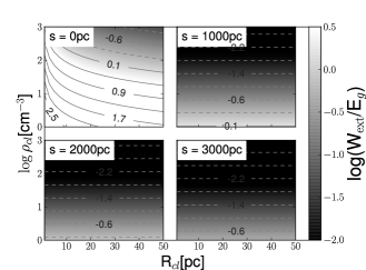
Figure 2.— $W_{\rm ext}/E_{g}$ map for constant density clouds of radius $R_{\rm cl}$ and density $\rho_{\rm cl}$, located inside a Galactic-type dark matter halo ($M=10^{12}\rm M_{\odot}$) and centered at a distance $s$ from the halo center. When the cloud center is located at the origin of the halo, its tidal energy can have a comparable effect to that of the gravitational energy. In general, the smaller and less dense clouds feel a greater gravitational contribution from the external medium.

Only clouds located very near the center of the halo feel a noticeable influence from it: the values for the energy ratio decay rapidly as the separation between the cloud and the halo increases. This is due to the central cuspiness of the NFW profile, shown in figure 1, since $W_{\rm ext}$ is dependent on the potential gradient which grows steeper near the origin. It is also evident that values of the tidal energy are more important for smaller and less dense clouds. Since the external gravity is “pulling” the particles in the cloud, it can be understood that a cloud of smaller diameter and lower density will be less tightly bound and easier to influence.

As a second example, we present the results from an identical estimate but for a dark matter halo of mass $10^{10}$ $\rm M_{\odot}$. In this case, the NFW parameters employed are $\rho_{s}=8.5\times 10^{-3}$ $\rm M_{\odot}$ pc^-3 and $r_{s}=3.8$ kpc. As in Fig. 2, in Fig. 3 we present the $\log{(W_{\rm ext}/E_{g})}$ maps for this halo’s characteristics. We notice that for a halo with these parameter values the effect is even weaker, and fades away faster as the molecular cloud moves away from the center of the halo. This smaller contribution can be explained as a result of the shallower potential well of this less massive halo.

It is important to mention that the ratios presented here only show the importance of the dark matter tidal energy compared to the gravitational energy of a cloud. We do not make any comparison with the gravitational influence of other possible matter components, such as a galaxy’s central black hole or star population. With the results shown, we conclude that a dark matter halo is only capable of influencing the evolution of small, diffuse clouds which are located near the center of massive galaxies.

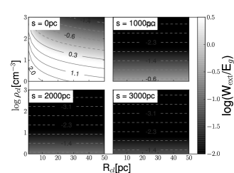
Figure 3.— As in Fig. 2 but for a galaxy with a halo mass of $10^{10}$ $\rm M_{\odot}$. A similar effect is noticed, but scaled down due to the potential well of such a halo being shallower.

4. GRAVITATIONAL FEEDBACK FROM A PERTURBED HALO

4.1. Perturbation Analysis

To continue with another perspective of the dark matter influence in a molecular cloud’s evolution, this and subsequent sections study the gravitational feedback effect that a perturbation on the local dark matter background (DMB), produced by a barionic cloud, has upon the energy budget of the cloud itself.

Dark matter interacts with barionic matter only gravitationally; as such, dark matter particles behave as a non-colissional fluid that feels a gravitational attraction to a mass distribution like a molecular cloud. Because galaxies are immersed in dark halos, a MC residing in it will coexist with a DMB. Following a dark halo distribution like that of NFW, this DMB would have an almost constant density at scales of the MC, because the variation scale of the halo’s density profile is much larger than the extent of even a giant molecular cloud (GMC). However, the mere presence of the barionic cloud perturbs the otherwise homogeneous DMB and promotes a density enhancement in it, which generates a potential well that will influence the MC in return. We analyze how important this perturbation can be to alter the evolution of a molecular cloud in different dark matter environments.

Although molecular clouds are highly irregular and structured (Combes, 1991; Ballesteros-Paredes et al., 2007, and references therein), we model them as Plummer spheres in order to follow up an analytical expression which may be easy to use. The mass distribution of such a sphere follows a density profile given by

$$\rho_{\rm cl}=\frac{3M_{\rm cl}}{4\pi a^{3}}\mathinner{\left(1+\frac{r^{2}}{a^{2}}\right)}^{-5/2},$$ (13)

where $M_{\rm cl}$ is the total mass of the cloud, $r$ is the radial distance from the center of the cloud, and $a$ is the scale-radius of the Plummer potential, which gives an idea of the size of the core of the distribution. The associated gravitational potential can be written as

$$\Phi_{\rm cl}(r)=-\frac{GM_{\rm cl}}{a}\frac{1}{\sqrt{1+r^{2}/a^{2}}},$$ (14)

where G is the gravitational constant. A cloud with these profiles is then placed within a DMB with constant density $\rho_{\rm DM}$ and a velocity dispersion $\sigma_{\rm DM}$.

Following Hernandez & Lee (2008), the dark matter particles are described by a Maxwell-Boltzmann velocity distribution function $f_{0}(v)\propto\exp(-v^{2}/2\sigma_{\rm DM}^{2})$. For the purpose of this study, the dark matter particles will have an average velocity of 0, that is, the DMB as a bulk is considered at rest with respect to the barionic matter. Although the gravitational potential of the dark matter halo $\Phi_{0}$ is constant at the scales of the molecular cloud, the MC induces a perturbation $\Phi_{1}$, so that the total potential $\Phi$ is the addition of both contributions, i.e.

$$\Phi(r)=\Phi_{0}(r)+\epsilon\Phi_{1}(r),$$ (15)

and the original density $\rho_{0}$ is enhanced by a perturbation $\rho_{1}$ and should become

$$\rho(r)=\rho_{0}+\epsilon\rho_{1}(r).$$ (16)

Similarily, the original Maxwell-Boltzmann distribution function $f_{0}(v)$ of the local dark matter halo gets perturbed by an amount $f_{1}(r,v)$ and the new distribution function will be given by

$$f(r,v)=f_{0}(v)+\epsilon f_{1}(r,v).$$ (17)

In order to know how the dark matter potential will be affected by the presence of the molecular cloud, we must solve the Boltzmann equation for non-collisional systems

$$\dfrac{\partial{}f}{\partial{t}}+\textbf{v}\cdot\nabla f-\nabla\Phi\cdot\nabla_{v}f=0,$$ (18)

in which $\nabla$ represents the gradient operator with respect to spatial coordinates and $\nabla_{v}$ the gradient operator with respect to velocity coordinates. The quantities involved in eq. (18) are the ones taking into account the perturbation caused by the barionic matter, i.e., the enhanced potential (eq. 15) and distribution function (eq. 17). For simplicity, we look for a first order stationary solution to the Boltzmann equation (i.e. $\partial{f}/\partial{t}=0$). By using the Jean’s swindle ($\Phi_{0}=0$), the fact that $f_{0}$ does not explicitly depend on the spatial coordinates ($\partial{f_{0}}/\partial{x_{i}}=0$), and considering only first order terms, the radial solution can be obtained as

$$\textbf{v}\cdot\nabla f = \nabla\Phi\cdot\nabla_{v}f,$$ (19)

$$= \nabla(\Phi_{0}+\Phi_{1})\cdot\nabla_{v}(f_{0}+f_{1}),$$

$$= \nabla\Phi_{1}\cdot\nabla_{v}f_{0}+\nabla\Phi_{1}\cdot\nabla_{v}f_{1},$$

$$\approx \nabla\Phi_{1}\cdot\nabla_{v}f_{0}.$$

We can calculate the gradient of the gravitational potential perturbation $\Phi_{1}$, which is actually the cloud potential $\Phi_{\rm cl}$, as

$$\dfrac{\partial{}\Phi_{1}}{\partial{r}}=\frac{GM_{\rm cl}}{a^{3}}\frac{r}{(1+r^{2}/a^{2})^{3/2}}.$$ (20)

Using the explicit form of the Maxwell-Boltzmann velocity distribution function to get the velocity gradient,

$$\dfrac{\partial{}f_{0}}{\partial{v}}=-\frac{v}{\sigma_{\rm DM}^{2}}f_{0}(v),$$ (21)

and after inserting the last two expressions in eq. (19), it becomes

$$v\dfrac{\partial{}f_{1}}{\partial{r}}=\frac{rGM_{\rm cl}}{a^{3}(1+{r^{2}}/{a^{2}})^{3/2}}\mathinner{\left(-\frac{v}{\sigma_{\rm DM}^{2}}\right)}f_{0}(v),$$ (22)

which furthermore, can be integrated over velocity space as

$$\dfrac{\partial{}\rho_{1}}{\partial{r}}=-GM_{\rm cl}\frac{r}{a^{3}(1+{r^{2}}/{a^{2}})^{3/2}}\mathinner{\left(\frac{1}{\sigma_{\rm DM}^{2}}\right)}\rho_{0}(v).$$ (23)

Remembering that the original DMB density has a constant value of $\rho_{\rm DM}$, this equation can be solved to yield

$$\rho_{1}=\frac{GM_{\rm cl}}{a\ \sigma_{\rm DM}^{2}}\frac{1}{\sqrt{1+{r^{2}}/{a^{2}}}}\rho_{\rm DM},$$ (24)

which is the density perturbation in the dark matter distribution produced by the molecular cloud. Such a density perturbation in the dark matter halo will produce its own non-constant gravitational field, which may, in principle, influence the gravitational energy budget of the molecular cloud. Our interest lies, thus, in the gravitational feedback of this enhancement over the cloud itself.

In order to calculate the tidal energy produced by the perturbed dark matter halo over the cloud, it is necessary to calculate the gradient of the gravitational potential $\phi_{\rm DM}$ associated to the perturbation $\rho_{1}$ given by eq. (24). The gravitational potential as a function of the radius $r$ that is produced by the perturbation $\rho_{1}$ will be given by

$$\phi_{\rm DM}(r) = -4\pi G\biggl{\{}\frac{1}{r}\int_{0}^{r}\rho_{1}(r^{\prime})r^{\prime 2}dr^{\prime}$$ (25)

$$+\int_{r}^{R_{\rm DM}}\rho_{1}(r^{\prime})r^{\prime}dr^{\prime}\biggr{\}},$$

integrated over the radial coordinate $r^{\prime}$ and where the second integral will be evaluated up to some radius $R_{\rm DM}$, such that the perturbation is fully contained within this radius, i.e. $R_{\rm DM}$ is taken such that $\rho_{1}(r=R_{\rm DM})=\rho_{0}$. Introducing (24) and integrating, we get an expression for the perturbed dark matter potential:

$$\phi_{\rm DM}(r) = -\frac{2\pi G^{2}M_{\rm cl}a}{\sigma_{\rm DM}^{2}}\rho_{\rm DM}\biggl{\{}(r/a)^{-1}\ln{\mathinner{\left(r/a+\sqrt{1+(r/a)^{2}}\right)}}$$ (26)

$$-\sqrt{1+(r/a)^{2}}+2\sqrt{1+(R_{\rm DM}/a)^{2}}\biggr{\}},$$

whose gradient is given by

$${\partial{\Phi_{\rm DM}}\over\partial r} = -\frac{4\pi G^{2}M_{\rm cl}a}{\sigma_{\rm DM}^{2}}\rho_{\rm DM}\biggl{\{}\frac{a\ln{\mathinner{\left(r/a+\sqrt{(r/a)^{2}+1}\right)}}}{2r^{2}}$$ (27)

$$-\frac{\sqrt{1+(r/a)^{2}}}{2r}\biggr{\}}.$$

Introducing this equation and the Plummer density distribution (13) into eq. (6), we obtain

$$W_{\rm ext}= - \frac{2\pi G^{2}aM_{\rm cl}^{2}\rho_{\rm DM}}{\sigma_{\rm DM}^{2}}\biggl{\{}\frac{2R/a}{1+(R/a)^{2}}-\arctan{\mathinner{\left(R/a\right)}}$$ (28)

$$- \frac{\ln{\mathinner{\left(R/a+\sqrt{1+(R/a)^{2}}\right)}}}{(1+(R/a)^{2})^{3/2}}\biggr{\}},$$

where $R$ is the truncation radius of the Plummer profile for the molecular cloud. This expression quantifies the tidal energy of the perturbed dark matter distribution over the cloud; in order to evaluate its importance in the process, it should be compared to the gravitational energy of the cloud itself, given by equation (3). Using eqs. (14) and (13) to evaluate this expression, the gravitational energy of the cloud becomes:

$$E_{\rm grav}=-\frac{3GM_{\rm cl}^{2}}{2a}\biggl{\{} \frac{R/a}{8\mathinner{\left(1+(R/a)^{2}\right)}}-\frac{R/a}{4\mathinner{\left(1+(R/a)^{2}\right)}^{2}}$$ (29)

$$+ \frac{1}{8}\arctan{\mathinner{\left(R/a\right)}}\biggr{\}}.$$

Thus, ratio of the gravitational to the tidal energy is

$$\frac{W_{\rm ext}}{E_{g}}=\mathinner{\left(\frac{a}{10\rm pc}\right)}^{2}\mathinner{\left(\frac{\rho_{\rm DM}}{\rm\rm M_{\odot}pc^{-3}}\right)}\mathinner{\left(\frac{\sigma_{\rm DM}}{\rm km\,s^{-1}}\right)}^{-2}f(R/a),$$ (30)

where we have defined

$$f(r/a)=-1.8025\ \ \frac{f_{\rm ext}(R/a)}{f_{g}(R/a)},$$ (31)

with

$$f_{\rm ext}(R/a)=\biggl{\{}\frac{2R/a}{1+(R/a)^{2}}-\arctan{\mathinner{\left(R/a\right)}}$$

$$-\frac{\ln{\mathinner{\left(R/a+\sqrt{1+(R/a)^{2}}\right)}}}{(1+(R/a)^{2})^{3/2}}\biggr{\}},$$ (32)

and

$${f_{g}(R/a)}=\frac{R/a}{8\mathinner{\left(1+(R/a)^{2}\right)}}-\frac{R/a}{4\mathinner{\left(1+(R/a)^{2}\right)}^{2}}$$

$$+\frac{1}{8}\arctan{\mathinner{\left(R/a\right)}}\biggr{\}}.$$ (33)

Equation (30) tells how important is a given dark matter environment on the gravitational energy budget of a molecular cloud. Several points must be stressed from this equation. First of all, the ratio of tidal to gravitational energy does not depend on the mass of the cloud, neither on its density. Furthermore, the tidal energy on the cloud produced by the perturbed halo will be more important for larger clouds, and larger background halo densities. On the other hand, for a halo’s larger velocity dispersion $\sigma_{\rm DM}$, the perturbation must be smaller and, as a consequence, the tidal energy will also be smaller, when compared to the gravitational energy, as showed by the $\sigma_{\rm DM}^{-2}$ dependence in eq. (30).

In Fig. 4 we plot the ratio $f$ vs $R/a$, as given by eqs. (31–33). Since the function is always positive, we note that the ratio of tidal to gravitational energy, eq. (30), will also be positive for any physically consistent combination of parameters $R/a$, $\rho_{\rm DM}$, $\sigma_{\rm DM}$. This means that the tidal energy caused by such a DMB will always contribute to the collapse of the MC perturbing it. This effect, when relevant, is expected to be reflected on the evolution of the cloud. In a molecular region forming stars, a rise in the compressional forces acting on it would show an increased star formation efficiency (SFE), as more stars will form faster when there is relatively less support against collapse. In the following section we explore the parameter space relevant to this scenario ($R/a$, $\rho_{\rm DM}$, $\sigma_{\rm DM}$).

Figure 4.— Ratio $f=f_{\rm ext}/f_{g}$ for a Plummer cloud of truncation size $R$ and characteristic scale $a$ = 10 pc. Note that the ratio is always positive, implying thus that the tidal energy always contributes to the collapse, according to eq. (30.)

4.2. Semi-analytical Results

In order to get an idea of the magnitude of the ratio $W_{\rm ext}/E_{g}$ in different dark matter environments, we need to provide dark matter backgrounds to the molecular clouds under study. As in section §3, we make use of the NFW model to estimate the structural parameters of the dark matter halos, where the MCs will be embedded. We need to determine the halo’s density $\rho_{\rm DM}$ and velocity dispersion $\sigma_{\rm DM}$, given its total mass $M_{\rm vir}$ and the radius $r$ at which these properties are evaluated, at a specified redshift $z$. We only consider here relatively nearby galaxies; that is, we assume redshift $z=0$.

To find $\rho_{\rm DM}$ and $\sigma_{\rm DM}$ we thus proceed as follows: for a given halo mass $M_{\rm vir}$, we obtain the concentration parameter $c$ following Bullock et al. (2001). With these values, we calculate its density profile parameters as specified in section §3. Once specified, we can evaluate the profile at the desired radius $r$ to know the local density $\rho_{\rm DM}$. On the other hand, in order to obtain $\sigma_{\rm DM}$, we adopt the relation given by Lokas & Mamon (2001, see their eq. 14) for the case where velocities of dark matter particles are considered isotropic. Such expression is dependent only on $c_{\rm vir}$, $M_{\rm vir}$ and $R_{\rm vir}$ and so the velocity dispersion obtained for a given halo is a constant. These recipes are used in our analysis to get the DMB parameters needed in different cases.

To begin with, we first choose parameters consistent with a Milky-Way type dark matter halo evaluated at a radius of 8 kpc, adequate to the solar neighborhood. However, in this case we preferred to use a more realistic concentration parameter $c=12$, closer to the observationally estimated value by, e.g., Battaglia et al. (2005). With these conditions, the procedure just described predicts a DMB with density $\rho_{DM}\sim 0.01\rm M_{\odot}$ pc^-3 and a velocity dispersion $\sigma_{\rm DM}=165$ km s^-1. With these parameters, equation (30) predicts that in order to get a non-negligible tidal effect ($W_{\rm ext}/E_{g}\sim 0.15$) the cloud’s scale radius $a$ has to be huge ($a=1900$ pc). A cloud of this size greatly surpasses the extent of local molecular clouds. On the other hand, since the energy ratio $W_{\rm ext}/E_{\rm grav}$ varies as $a^{2}$, we note that for more typical clouds, $a\sim 10$ pc and $R/a\sim 10$, the contribution of the tidal energy is negligible.

Figure 5 presents a more interesting case in which the energy ratio is non-negligible for a range of cloud sizes $R/a$. The cloud has a Plummer radius of $a=10$ pc and it is embedded in a dark matter halo with mass $M=10^{7}\,\rm M_{\odot}$ at a distance of $r=0.1r_{s}$.

Figure 5.— $W_{\rm ext}/E_{g}$ ratio for a cloud of Plummer radius $a=10$ pc and different truncation radii (R), embedded in a dark matter halo typical of dwarf galaxies ($M\sim 10^{7}\rm M_{\odot}$), at a radius $r=0.1r_{s}$. In this case, even small molecular clouds would feel a a non-zero tidal effect from their environment.

We can see, in this case, that even small clouds of the order of 10 pc will feel a non-zero tidal effect from the dark matter environment.

Figure 6 shows, in grey scale, the energy ratios $W_{\rm ext}/E_{g}$ evaluated using a NFW dark matter density profile with a range of velocity dispersions $\sigma_{\rm DM}$ and densities $\rho_{\rm DM}$. In this figure, the parameters of the Plummer cloud are $a=$10 pc, and $R/a=10$. Similar maps are presented in Figs. 7 and 8, but for clouds with $R/a=5$ and 1, respectively. As a reference, in these images we also indicate the typical densities and velocity dispersions of dark matter halos of galaxies with total masses ranging from $10^{7}$ to $10^{11}~{}\rm M_{\odot}$. Density profiles are computed at $r=0.1r_{s}$.

Figure 6.— $W_{\rm ext}/E_{g}$ map for Plummer clouds with characteristic radius $a=10$ pc and $R/a$=10, embedded in a homogeneous dark matter background of parameters $\rho_{\rm DM}$ and $\sigma_{\rm DM}$. The tidal energy can contribute to the collapse of clouds immersed in dwarf galaxies. As the energy ratio increases as $a^{2}$, also massive galaxies can show this effect for large enough MCs.

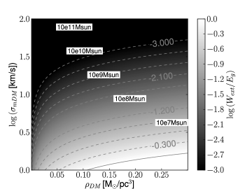
Figure 7.— Same as in Fig. 6, but for $R/a$=5. The differences with Fig. 6 are not significant because Plummer spheres contain most of their mass within 5 characteristic radii.

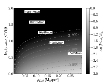
Figure 8.— Same as in Fig. 6, but for $R/a$=1. In this case, the tidal effect is diminished when compared to Fig. 6 because we are considering a more concentrated sphere in which the tidal forces have more difficulties to act.

Two points can be highlighted from Fig. 6. First, the tidal energy of the dark matter halo becomes important for large clouds ($R\sim 100$ pc) in galaxies with masses ranging from 10⁷ to 10⁸ $\rm M_{\odot}$. Secondly and as noticed previously, since the ratio $W_{\rm ext}/E_{\rm grav}$ scales as $a^{2}$, this contribution become important also in larger galaxies for large enough clouds. For instance, as can be inferred from Fig. 7, $\sim$ 10% of the total gravitational energy content of a giant cloud complex ($a\sim 100$ pc, $R\sim$ 0.5 kpc) embedded in a 10¹⁰ $\rm M_{\odot}$ dark matter halo will be due to the tidal compression energy produced by the potential well induced by the cloud itself.

The high similarity between Figs. 6 and 7 is likely due to the mass of a Plummer sphere being concentrated in the inner 5 characteristic radii (93% of the mass of the distribution lies at $r<4a$). On the other hand, Figure 8, which shows the case $R/a=1$, does show smaller contributions from the environment to the energy budget of the cloud than those shown in previous figures. The reason can be traced again to the inherent concentration of a Plummer sphere: as we truncate the sphere at $r=a$, we are only considering the inner core of the cloud, which has a higher gravitational energy and in which the tidal contribution has more trouble to act.

To further study the “big cloud” scenario, a different exploration of parameters is shown in Figure 9, in which the density and velocity dispersion of the dark matter background are set according to the theoretical values of a Milky Way-type halo, at a radius of 50 kpc ($\rho_{\rm DM}=0.0002~{}\rm M_{\odot}$pc^-3, $\sigma_{\rm DM}=150$ km s^-1), while the cloud characteristic radius $a$ and truncation radius $R$ are varied. This allows us to identify the characteristics of a mass distribution that would suffer a relevant contraction by the tidal forces: the figure shows that, for a radius larger than $\sim 8000$ pc ($a=8000$ pc, $R/a=1$, or $a=6000$ pc, $R/a=1.3$) and located at some 50 kpc from the center of the Milky Way, it will produce a perturbation in the dark matter halo which will in turn have a small contribution to the gravitational energy it contains (around 1%). This location and dimensions are similar to that of a satellite galaxy like the Large Magellanic Cloud. The effect is indeed low, but the theoretical implications it suggests are interesting, as we could say that at least some contribution to the star formation seen in orbiting galaxies or in galaxy mergers could come from the tidal energy caused by a dark matter perturbation.

Figure 9.— $W_{\rm ext}/E_{g}$ map for Plummer clouds of characteristic radius $a$ and truncation radius $R$, embedded in a homogeneous dark matter background with density and velocity dispersion corresponding to a Milky Way dark matter halo at 50 kpc from its center ($\rho_{\rm DM}=0.0002~{}\rm M_{\odot}$pc^-3, $\sigma_{\rm DM}=150$ km s^-1). A big mass distribution (like a satellite galaxy) would feel a small tidal energy contribution.

Still, one more scenario to consider is that of a cloud closer to the center of a galaxy Milky-Way type. In Figure 10, the dark matter parameters are fixed to fit the Milky Way’s dark matter halo at 2 kpc from its center ($\rho_{\rm DM}=0.04~{}\rm M_{\odot}$pc^-3, $\sigma_{\rm DM}=150$ km s^-1), while the cloud dimensions are explored. Note that in this case, a large cloud complex of $a\sim 1$ kpc and $R\sim 2$ pc will have a tidal energy ($\sim 6\%$) that will slightly contribute to its collapse. This possibility suggests that a complex like the molecular ring in the Mily Way may be affected somehow by the tidal energy produced by the perturbation in the halo that the cloud complex imprints on it.

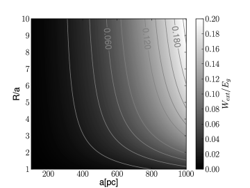
Figure 10.— Same as in Fig. 9, but for a Milky Way dark matter halo at 2 kpc from its center ($\rho_{\rm DM}=0.04~{}\rm M_{\odot}$pc^-3, $\sigma_{\rm DM}=150$ km s^-1). In this case, a large cloud complex would suffer a tidal effect from the dark matter, compared to the previous case.

5. NUMERICAL SIMULATIONS OF CLOUD FORMATION WITHIN A DM HALO

Different studies support the idea that molecular clouds in the Milky Way are transient entities produced by compressions from large scale streams in the interstellar medium (Ballesteros-Paredes et al., 1999a, b; Hartmann et al., 2001; Vázquez-Semadeni et al., 2007; Heitsch & Hartmann, 2008; Vázquez-Semadeni et al., 2010). On the other hand, in sections 4.1 and 4.2 we derived semi-analytical calculations which suggest that a dark matter well produced by the perturbation of a barionic distribution of mass can significantly add to its gravitational budget, and thus contribute to its collapse, if the right conditions are given. In order to test this scenario within a more realistic setting, we have performed a series of numerical experiments in which a dense cloud is formed by the collision of two streams of diffuse gas. The colliding gas cools down, becomes denser and collapses. While doing so, the collapsing cloud perturbs the locally homogeneous dark matter halo in which it is embedded, producing a potential well. This will give an extra tidal energy contribution to the original cloud, which is expected to translate into a larger star formation activity. Given the differences between the semi-analytical and the numerical circumstances (initial conditions and treatment), we do not expect semi-analytical results to faithfully reflect the behavior of the gas and dark matter in the simulations; still, the gravitational feedback effect must appear in the simulations. This effect can be then estimated in the numerical experiments through the comparison of the cloud’s star formation efficiency with and without dark matter.

To perform the simulations, we use the Adaptive Refinement Tree (Kravtsov et al., 1997; Kravtsov, 2003) code (ART), which employs an $N-$body algorithm to solve the gravitational interactions of the system. The chosen version of the code additionaly solves gas hydrodynamics and can handle radiative cooling and star formation, as presented by Vázquez-Semadeni et al. (2010).

The initial conditions for the gas are taken from previous star formation simulations by Vázquez-Semadeni et al. (2010). We consider a 256 pc-per-side box filled with tenuous gas ($n_{0}=1$ cm^-3) at a temperature of $T_{0}=5000$ K, which represents a warm neutral hydrogen medium (molecular weight $\mu_{0}=1.27$). The gas has an inital turbulent velocity fluctuation distribution of magnitude $v_{\rm rms}=0.1$ km s^-1  everywhere. On top of that, two gas streams moving towards each other along the $x-$axis are created by adding an initial velocity component of 7.5 km s^-1, to the material contained in two 112 pc long cylinders with radii of 64 pc, lying on each side of the box. Since the sound speed for the gas amounts to $c_{s}=7.4$ km s^-1, the flows are trans-sonic. The gas that comprises the streams constitutes less than 20% of the total mass in the box. The cloud evolution is followed during 40 Myr.

The local dark matter background is represented by particles that interact only gravitationally, both with other dark matter particles and with the gas. Table 1 shows in the first and second column the values of the density $\rho_{\rm DM}$ and the velocity dispersion $\sigma_{\rm DM}$, respectively, used in each simulation. These were calculated following the schemes described in section 6. In the third column, we show the typical mass of a halo (galaxy) associated with those $\rho_{\rm DM}$ and $\sigma_{\rm DM}$ values, given at the radius shown in the fourth column.

Table 1Variable parameters in the simulations

$\rho_{\rm DM}$	$\sigma_{\rm DM}$	log($M_{\rm vir}$	$r/r_{s}$	Linestyle
($\rm M_{\odot}$pc-3)	(km s-1)	$\rm[\rm M_{\odot}]$)		in Fig. 12
0	0	(…)a	(…)a	solid
0.1	37	10	0.15	dashed
0.1	10	8	0.26	long-dashed
0.1	2	(…)b	(…)b	dash-dotted
0.1	1	(…)b	(…)b	dotted
0.17	3.16	7	0.13	dot-long dashed
0.24	3.16	7	0.1	short-log dashed

Note. — Dark matter density ($\rho_{\rm DM}$) and vel. dispersion ($\sigma_{\rm DM}$) are shown, as well as the mass of a galaxy ($M_{\rm vir}$) whose characteristic NFW halo represents these values at the radius ($r$) given, when applicable.

To decouple the effect of the dark matter background on the behavior of the gas from other effects, we need to study its evolution without a dark matter background. This reference run was taken from Vázquez-Semadeni et al. (2010) (SAF0, which stands for Small Amplitude Fluctuations without stellar feedback) and it has the same values of the gas parameters described above. These authors report the formation of a “central cloud” of irregular shape with a radius of the order of 10 pc, where star formation is concentrated. Although the physical configuration of the simulation differs from the one of the analytical case we studied previously, we believe it is a good test case for investigating the general effect: the promotion of a higher star formation rate.

In order to quantify the differencees in the evolution of the different runs, we calculated the Star Formation Efficiency (SFE) as defined by, for example, Vázquez-Semadeni et al. (2010):

$${\rm SFE}=\frac{M_{*}}{M_{*}+M_{\rm gas}},$$ (34)

where $M_{*}$ represents the mass contained in stars and $M_{\rm gas}$ accounts for the mass in the dense gas ($n\mathrel{\mathchoice{\lower 0.5pt\vbox{\halign{$\mathnew\displaystyle\hfil#\hfil$\cr>\crcr\sim\crcr}}}{\lower 0.5pt\vbox{\halign{$\mathnew\textstyle\hfil#\hfil$\cr>\crcr\sim\crcr}}}{\lower 0.5pt\vbox{\halign{$\mathnew\scriptstyle\hfil#\hfil$\cr>\crcr\sim\crcr}}}{\lower 0.5pt\vbox{\halign{$\mathnew\scriptscriptstyle\hfil#\hfil$\cr>\crcr\sim\crcr}}}}10^{2}\ \mbox{cm${}^{-3}$}$), at any given moment during the evolution of the system. We also compute the relative difference between the SFE of any run with dark matter and the reference run (without it), at any given time, $\Delta$; that is,

$$\Delta=\frac{{\rm SFE}_{\rm ref}-{\rm SFE}_{\rm run}}{\rm SFE_{\rm ref}}.$$ (35)

In this context, the first point to clarify is whether these variables allow us to distinguish between the evolution of runs with different physics (e.g., no dark matter included vs. a particular configurations of dark matter halos), and the evolution of runs with the same physics, but different initial fluctuations. Thus, in Fig. 11, we show the time evolution of the SFE (upper panel) for three runs with identical physics (with dark matter properties $\rho_{\rm DM}=0.24\rm M_{\odot}$pc^-3, $\sigma_{\rm DM}=3.16$ km s^-1), but with different phases for the initial density and velocity fluctuations. However, in this case and unlike explained before, what is drawn as $\Delta$ in the lower panel of Fig. 11 is the relative difference between the SFE of the run plotted with a solid line and the runs plotted with a dashed or a dotted line (which differ only in the phase of the initial conditions). As can be seen in this figure, the differences among the three runs are not large, so the different initial conditions do not constitute a significant source for variations in the SFE. Thus, if any of our performed runs with dark matter produces substantially larger differences, it must be due mainly to the gravitational influence of the dark matter.

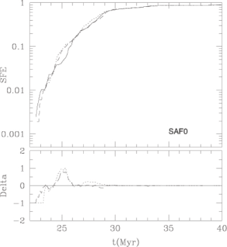
Figure 11.— SFE and differential values (with respect to the solid line run) for three different runs with different random phases of the initial density and velocity field, but otherwise identical physical conditions: $\rho_{\rm DM}=0.24\rm M_{\odot}$pc^-3,$\sigma_{\rm DM}=3.16$ km s^-1. As can be noticed, the differences are not large. Thus, for runs with dark matter halo, any difference substantially larger than these shown in this figure will be considered as representative of the gravitational influence of the dark matter halo.

6. NUMERICAL RESULTS

As commented above, the collision of the streams in the simulations develops instabilities in the atomic gas which changes its phase and becomes molecular material with lower temperatures and higher densities; this new phase forms condensations that grow with time. As the shocked region increases its mass, the cloud starts contracting. The star formation starts at $\sim$ 25 Myr after the begining of the simulation, and has a rapid growth soon after. Around 10 Myr later, most of the gas in the simulation box has been transformed into stars and hence the SFE approaches its maximum possible value of 1 (see Fig. 12).

In Figure 12 we show the time evolution of the SFE (upper panels) and $\Delta$ (lower panels) for the different runs outlined in Table 1, as compared to the reference run, which is shown as a solid line in all panels. On the left side we present the runs with density $\rho_{\rm DM}=0.1\rm M_{\odot}$pc^-3 and velocity dispersions $\sigma_{\rm DM}=37$ km s^-1 (dashed line) and $\sigma_{\rm DM}=10$ km s^-1 (long-dashed line). Aside from the initial fluctuations, these runs show no significant difference in the evolution of the SFE, as compared to the reference run (solid line). This behavior is consistent with the results predicted for $W_{\rm ext}/E_{\rm grav}$ by our semi-anlytical approach (see Figs. 6, 7 and 8). As far as the SFE is concerned, these simulations proceeded as if the dark matter was not present.

Figure 12.— SFE and $\Delta$ values for the simulation runs described in Table 1. The reference run is displayed as the solid line in all three panels. The left panel compares high velocity dispersion DMBs ($\sigma_{\rm DM}\geq 10$ km s^-1) with the reference run. Both runs in this panel have a density of $\rho_{\rm DM}=0.1\rm M_{\odot}$pc^-3: the dashed line shows the run with $\sigma_{\rm DM}=37$ km s^-1, while the long-dashed line depicts the one with $\sigma_{\rm DM}=10$ km s^-1. No significant difference is found from the reference run, as expected from the analytical predictions. The central panel shows two more runs with the same density ($\rho_{\rm DM}=0.1\rm M_{\odot}$pc^-3) but smaller velocity dispersions: $\sigma_{\rm DM}=2$ km s^-1 (dash-dotted line) and $\sigma_{\rm DM}=1$ km s^-1 (dotted line). These cases show a systematically higher SFE than the reference run, also as expected. Two more runs with higher densities are displayed on the right panel: $\rho_{\rm DM}=0.17\rm M_{\odot}$pc^-3, $\sigma_{\rm DM}=3.16$ km s^-1 (dot-long dashed line) and $\rho_{\rm DM}=0.24\rm M_{\odot}$pc^-3, $\sigma_{\rm DM}=3.16$ km s^-1 (short-long dashed line). Again, the star formation seems a lot more active than the reference run.

The central panel depicts two more runs with the same density ($\rho_{\rm DM}=0.1\rm M_{\odot}$pc^-3) but with lower velocity dispersions: $\sigma_{\rm DM}=2$ km s^-1 (dash-dotted line) and $\sigma_{\rm DM}=1$ km s^-1 (dotted line). In this cases, there is a marked difference in the overall evolution of the SFE. The $\sigma_{\rm DM}=2$ km s^-1 run distinguishes from the previous ones in that its SFE is consistenly higher than the one of the reference; there is a period of time in which it has an SFE a factor of two higher than the reference value. The dotted line in the same panel has an SFE that is systematicaly higher than all previous runs. It can clearly be seen that runs with lower dark matter velocity dispersions (density remaining constant) produce higher SFEs. As can be deduced from Figure 7, an important contribution is expected from the external gravitational potential towards the collapse of the cloud: a ratio $W_{\rm ext}/E_{g}$ in the range  0.3-0.8 for these cases. This translates into a significant enhancement of the star formation rate. The right panel, in the same Fig. 12, shows two other cases. These runs have both a higher density than those runs considered in the left and middle panels. One run has $\rho=0.17\rm M_{\odot}$pc^-3 (dot-long dashed line) and the other one $\rho=0.24\rm M_{\odot}$pc^-3 (short-long dashed line). They are simulated with the same velocity dispersion $\sigma_{\rm DM}=3.16$ km s^-1. These models also show an enhanced SFE in comparison to the reference run, but here the contribution due to the DMB seems somewhat larger than the expected from the analytical predictions (see Figs. 6, 7 and 8). Such a deviation is, however, not surprising: the predicted external contribution comes from an ideal model that considers a spherical molecular cloud at rest, while the simulation contains more realistic conditions.

7. DISCUSSION AND CONCLUSIONS

We investigated the effect that the gravitational contribution from dark matter, in the form of tidal energy, has on the energy balance of a molecular cloud and its evolution. On considering the large-scale dark matter halos, where galaxies are supposed to be immersed, we noticed that there is an important gravitational contribution only for clouds very near to the center of these halos, specially for low-density, small molecular clouds. The effect of this collapse-promoting force dissapears very rapidly as the cloud location is moved away from the center. To our knowledge, this effect has not been studied before, perhaps in part because clouds were not expected to be affected by the presence of the dark matter. In light of these results, these predictions can be applied to structures encountered in the central region of galaxies. In fact, Genzel et al. (1990) report on a series of observations regarding the rich gas structure in the inner 10 pc of the Milky Way, comprised of a couple giant molecular clouds, a circumnuclear disk and an HII region. These entities lie at the right position, are small and clumpy (averaging $\sim 3$ pc in diameter) and span a large range of densities (Vollmer, B. & Duschl, W. J., 2002). Such gas distributions can, according to our results, be feeling a great gravitational compression from the external medium, relative to their self-gravity. These results also suggest that the intense star formation activity found in the innermost regions of large galaxies (like ours) may have some contribution from tidal compression caused by the dark matter halo of the galaxy.

In this particular case, the presence of the central black hole (with an estimated mass $M_{\rm BH}=4\times 10^{6}\rm M_{\odot}$; Schoedel et al., 2002) is only relevant when the molecular cloud structure reaches distances smaller than $\sim 1$ pc, in accordance with the radius of influence of a central black hole $r_{h}=GM_{\rm BH}/v_{0}$ (where $v_{0}$ is the velocity dispersion of stars at the center; Peebles, 1972, for our Galaxy, $r_{h}\approx 0.5$ pc). Following the same analysis presented here to set an example, we estimate that the gravitational energy contribution ($W_{\rm BH}$) that the Milky Way’s central black hole excerts on a 3 pc diameter cloud with density $n=10^{3}$ cm^-3, located 5pc away from the center of the Galaxy is given by $W_{\rm BH}/E_{g}<0.01$, which is not significant in comparison to the dark matter contribution.

On the other hand, the local dark matter background permeating a molecular cloud is shown to be able to contribute to its star formation if the appropriate conditions are fulfilled. The high dark matter densities and low velocity dispersions, found in dwarf spheroidal galaxies, needed for the tidal energy to be important for the evolution of molecular clouds are not expected in galaxies where there is a significant amount of molecular gas; namely, spiral and irregular galaxies. Yet, small galaxies dominated by dark matter with a significant fraction of gas are not ruled out. Moreover, although the Solar Neighborhood does not meet the dark matter conditions where star formation would be greatly enhanced by its presence, we predict a small contribution for big clouds.

This work has shown that despite the huge difference between the length scales of molecular clouds and dark matter halos, the latter could influence the evolution of a star forming region. We show that this effect is negligible in our local environment, but that it can have possible applications in other environments, other locations or other galaxies. In summay, our study firmly suggests that the external dark matter gravitational contribution should be considered, when analyzing the dynamical evolution of a molecular cloud, if the right conditions are fullfilled.

References

- Ballesteros-Paredes (2006) Ballesteros-Paredes, J. 2006, MNRAS, 372, 443
- Ballesteros-Paredes et al. (2009a) Ballesteros-Paredes, J., Gómez, G. C., Loinard, L., Torres, R. M., & Pichardo, B. 2009a, MNRAS, 395, L81
- Ballesteros-Paredes et al. (2009b) Ballesteros-Paredes, J., Gómez, G. C., Pichardo, B., & Vázquez-Semadeni, E. 2009b, MNRAS, 393, 1563
- Ballesteros-Paredes et al. (1999a) Ballesteros-Paredes, J., Hartmann, L., & Vázquez-Semadeni, E. 1999a, ApJ, 527, 285
- Ballesteros-Paredes et al. (2011a) Ballesteros-Paredes, J., Hartmann, L. W., Vázquez-Semadeni, E., Heitsch, F., & Zamora-Avilés, M. A. 2011a, MNRAS, 411, 65
- Ballesteros-Paredes et al. (2007) Ballesteros-Paredes, J., Klessen, R. S., Mac Low, M.-M., Vazquez-Semadeni, E. 2007, in Protostars and Planets V, ed. V, B. Reipurth, D. Jewitt, & K. Keil (Tucson, AZ: Univ. Arizona Press), 63
- Ballesteros-Paredes et al. (1999b) Ballesteros-Paredes, J., Vázquez-Semadeni, E., & Scalo, J. 1999b, ApJ, 515, 286
- Ballesteros-Paredes et al. (2011b) Ballesteros-Paredes, J., Vázquez-Semadeni, E., Gazol, A. et al. 2011b, MNRAS, 416, 1436
- Battaglia et al. (2005) Battaglia, G., Helmi, A., Morrison et al. 2005, MNRAS, 364, 433
- Bullock et al. (2001) Bullock, J. S., Kolatt, T. S., Sigad, Y. et al. 2001, MNRAS, 321, 559
- Burkert & Hartmann (2004) Burkert, A., & Hartmann, L. 2004, ApJ, 616, 288
- Combes (1991) Combes, F. 1991, ARAA, 29, 195
- Gavazzi et al. (2003) Gavazzi, R., Fort, B., Mellier, Y., Pelló, R., & Dantel-Fort, M. 2003, A&A, 403, 11
- Genzel et al. (1990) Genzel, R., Stacey, G. J., Harris, A. I. et al. 1990, ApJ, 356, 160
- Gómez et al. (2007) Gómez, G. C., Vázquez-Semadeni, E., Shadmehri, M., & Ballesteros-Paredes, J. 2007, ApJ, 669, 1042
- Hartmann et al. (2001) Hartmann, L., Ballesteros-Paredes, J., & Bergin, E. A. 2001, ApJ, 562, 852
- Heitsch & Hartmann (2008) Heitsch, F., & Hartmann, L. 2008, ApJ, 689, 290
- Hernandez & Lee (2008) Hernandez, X., & Lee, W. H. 2008, MNRAS, 387, 1727
- Kravtsov (2003) Kravtsov, A. V. 2003, ApJL, 590, L1
- Kravtsov et al. (1997) Kravtsov, A. V., Klypin, A. A., & Khokhlov, A. M. 1997, ApJS, 111, 73
- Lokas & Mamon (2001) Lokas, Ewa L. & Mamon, Gary A. 2001, MNRAS, 321, 155
- McKee & Zweibel (1992) McKee, C. F., & Zweibel, E. G. 1992, ApJ, 399, 551
- Myers & Goodman (1988a) Myers, P. C., & Goodman, A. A. 1988a, ApJL, 326, L27
- Myers & Goodman (1988b) Myers, P. C., & Goodman, A. A. 1988b, ApJ, 329, 392
- Navarro et al. (1996) Navarro, J. F., Frenk, C. S., & White, S. D. M. 1996, ApJ, 462, 563
- Peebles (1972) Peebles, P. J. E. 1972, ApJ, 178, 371
- Schoedel et al. (2002) Schoedel, R. et al. 2002, Nature, 419, 694
- Shu (1992) Shu, F. H. 1992, The Physics of astrophysics. Volume II: Gas dynamics, University Science Books, Chapter 24
- Shu et al. (1987) Shu, F. H., Adams, F. C., & Lizano, S. 1987, ARAA, 25, 23
- Vázquez-Semadeni (2010) Vázquez-Semadeni, E. 2010, ASPC, 48, 83
- Vázquez-Semadeni et al. (2010) Vázquez-Semadeni, E., Colín, P., Gómez, G. C., Ballesteros-Paredes, J., & Watson, A. W. 2010, ApJ, 715, 1302
- Vázquez-Semadeni et al. (2007) Vázquez-Semadeni, E., Gómez, G. C., Jappsen, A. K. et al. 2007, ApJ, 657, 870
- Vollmer, B. & Duschl, W. J. (2002) Vollmer, B., Duschl, W. J. 2002, A&A, 388, 128