Reduced Collocation Methods: Reduced Basis Methods in the Collocation Framework

Abstract

In this paper, we present the first reduced basis method well-suited for the collocation framework. Two fundamentally different algorithms are presented: the so-called Least Squares Reduced Collocation Method (LSRCM) and Empirical Reduced Collocation Method (ERCM). This work provides a reduced basis strategy to practitioners who prefer a collocation, rather than Galerkin, approach. Furthermore, the empirical reduced collocation method eliminates a potentially costly online procedure that is needed for non-affine problems with Galerkin approach. Numerical results demonstrate the high efficiency and accuracy of the reduced collocation methods, which match or exceed that of the traditional reduced basis method in the Galerkin framework.

1 Introduction

Reduced basis methods (RBM) [2, 14, 16, 18, 19, 7] were developed for scenarios that require a large number of numerical solutions to a parametrized partial differential equation in a fast/real-time fashion. Examples of such situations include simulation-based design, parameter optimization, optimal control, multi-model/scale simulation etc. In these situations, we are willing to expend significant computational time to pre-compute data that can be later used to compute accurate solution in real-time.

The RBM splits the solution procedure into two parts: an offline part where the parameter dependence is examined and a greedy algorithm is utilized to judiciously select $N$ parameter values for pre-computation; and an online part when the solution for any new parameter is efficiently computed based on these $N$ basis functions.

The motivation behind the RBM is the recognition that parameter-induced solution manifolds can be well approximated by finite-dimensional spaces. For linear affine problems, RBM can improve efficiency by several orders of magnitude. For nonlinear or non-affine problems, there are remedies which allow the RBM methods to be used efficiently [3, 9, 15]. The offline selection of the $N$ parameter values for the pre-computed bases is enabled by a rigorous a posteriori error estimate which guarantees the accuracy of the solution. Exponential convergence with respect to $N$ has been commonly observed, see [19, 7] and the reference therein. Theoretically, a priori convergence is confirmed for a one dimensional parametric problem [13]. More recently, exponential convergence of the greedy algorithm for continuous and coercive problems with parameters in any dimension has been established in [5], and improved in [4].

The development and analysis of RBM has been previously carried out in the Galerkin framework. That is, the truth approximations (the numerical approximation from a presumably very accurate numerical scheme) are obtained from a (Galerkin) finite element method, and the reduced basis solution is sought as a Galerkin projection onto a low dimensional space. However, to date RBM have not been developed, applied, or analyzed in the context of collocation methods. While Galerkin methods are derived by requiring that the projection of the residual onto a prescribed space is zero, collocation methods require the residual to be zero at some pre-determined collocation points. Compared to collocation methods, Galerkin methods have a weaker regularity requirement on the solution. For example, for second-order problems, collocation methods require the solution to be at least $H^{2}$ over the domain $\Omega$, while Galerkin methods only require solutions in $H^{1}(\Omega)$, due to the adoption of the weak formulation. Unlike collocation methods, Galerkin methods do not require a tensorial grid and handle curved boundaries with ease. On the other hand, collocation methods are particularly attractive for their ease of implementation, particularly for time-dependent nonlinear problems [21, 20, 10].

In this paper, we develop the RBM idea for collocation methods. Given a highly accurate collocation method that is used as the truth solver for the parametric problem, we wish to study the performance of the system under variation of certain parameters using a collocation-based RBM. That is, the new method uses collocation for both the truth solver and the online reduced solver.

The paper is organized as follows. In Section 2, we present two approaches to collocation RBM. The first one utilizes a least squares approach. The second one relies on a projection of the fine collocation grid problem onto a (carefully-chosen) coarse collocation grid. Theoretical analysis and discussions on the offline-online decomposition are provided in Section 3. Numerical results are shown in Section 4. Finally, some concluding remarks and future directions are in Section 5.

2 The Algorithms

We begin with a parametrized partial differential equation of the form

$$\mathbb{L}(\mu)\,u_{\mu}(x)=f(x;\mu),\qquad x\in\Omega\,\,\,{\color[rgb]{0,0,0}\subset\mathbb{R}^{n}}$$ (1)

with appropriate boundary conditions. We are interested in the solutions of the differential equation over a range of parameter values $\mu$, where $\mu=(\mu_{1},\dots,\mu_{d})\in{\mathcal{D}}$, a prescribed $d$-dimensional real parameter domain. The parameters can be, for example, heat conductivity, wave speed, angular frequency, or geometrical configurations etc.

In this work, we assume that the operator is linear and affine with respect to functions of $\mu$. That is, $\mathbb{L}(\mu)$ can be written as a linear combination of parameter-dependent coefficients and parameter-independent operators:

$$\mathbb{L}(\mu)=\sum_{q=1}^{Q_{a}}a^{\mathbb{L}}_{q}(\mu)\mathbb{L}_{q}.$$ (2)

We make a similar assumption for $f$:

$$f(x;\mu)=\sum_{q=1}^{Q_{f}}a^{f}_{q}(\mu)f_{q}(x).$$ (3)

In the Galerkin framework, these are common assumptions in the reduced basis literature [19]. There are remedies available when the parameter-dependence is not affine [3, 9, 15].

For any value of the parameter $\mu$, we can approximate the solution to this equation using a collocation approach: we define a discrete differentiation operator $\mathbb{L}_{\mathcal{N}}(\mu)$ so that the approximate solution $u^{\mathcal{N}}_{\mu}$ satisfies the equation

$$\mathbb{L}_{\mathcal{N}}(\mu)\,u^{\mathcal{N}}_{\mu}(x_{j})=f(x_{j};\mu),$$ (4)

exactly on a given set of ${\mathcal{N}}$ collocation points $C^{\mathcal{N}}=\{x_{j}\}_{j=1}^{\mathcal{N}}$, usually taken as a tensor product of ${\mathcal{N}}_{x}$ collocation points for each dimension. Obviously, for $\Omega\subset\mathbb{R}^{n}$ we have ${\mathcal{N}}={\mathcal{N}}_{x}^{n}$. We assume that the scheme (4) produces highly accurate numerical solutions $u^{\mathcal{N}}_{\mu}$ to the problem (1). We refer to the solution $u^{\mathcal{N}}_{\mu}$ as the “truth approximation”.

Although solving (4) gives highly accurate approximations, it is prohibitively expensive and time-consuming to repeat for a very large number of parameter values $\mu$. The reduced basis method allows for highly accurate solutions to be computed quickly and efficiently when needed (the “online” computation) based on a set of possibly expensive offline computations. The idea of the reduced basis method is that we first pre-compute the truth approximations for a set of $N<<{\mathcal{N}}$ well-chosen parameter values $\{\mu^{1},\,\mu^{2},\,\dots,\,\mu^{N}\}$ by solving (4) with the corresponding parameter value. Then when the solution for any parameter value $\mu^{*}$ in the (prescribed) parameter domain ${\mathcal{D}}$ is needed, instead of solving for the (usually expensive) truth approximation $u^{\mathcal{N}}_{\mu^{*}}$, we combine $u^{\mathcal{N}}_{\mu^{1}},\,u^{\mathcal{N}}_{\mu^{2}},\,\dots,\,u^{\mathcal{N}}_{\mu^{N}}$ in some way to produce a surrogate solution $u^{(N)}_{\mu^{*}}$:

$$u^{(N)}_{\mu^{*}}=\sum_{j=1}^{N}c_{j}(\mu^{*})u^{\mathcal{N}}_{\mu^{j}}.$$

Thus, the design of the reduced basis method requires two components:

1. Offline: how to select the pre-computed basis.

2. Online: how to combine the pre-computed basis functions to produce the surrogate solution.

In the following sections, we describe two variants of the reduced collocation algorithm. We first explain our approaches for the online computation of the surrogate solution from the pre-computed reduced basis in Section 2.1, and then the related question of the selection of the reduced basis in Section 2.2.

2.1 Online algorithms

For the surrogate solution $u^{(N)}_{\mu^{*}}$ to approximate the truth approximation $u^{\mathcal{N}}_{\mu^{*}}$ reasonably well, we require that $u^{(N)}_{\mu^{*}}$ provides, in some sense, a good approximation to the solution of the discretized differential equation

$$\mathbb{L}_{\mathcal{N}}(\mu^{*})\left(\sum_{j=1}^{N}c_{j}u^{\mathcal{N}}_{\mu^{j}}\right)\approx f(x;\mu^{*}).$$

By exploiting the linearity of the operator we observe that our task is to find coefficients $c_{j}(\mu^{*})$ so that the residual

$$\sum_{j=1}^{N}c_{j}(\mu^{*})\mathbb{L}_{\mathcal{N}}(\mu^{*})u^{\mathcal{N}}_{\mu^{j}}-f(x;\mu^{*})$$

is small.

In the Galerkin framework [19, 7], the coefficients are found by requiring that the $L^{2}$-projection of this residual onto the reduced space is zero. For the collocation case, the system of equations we wish to solve is

$$\sum_{j=1}^{N}c_{j}(\mu^{*})\mathbb{L}_{\mathcal{N}}(\mu^{*})u^{\mathcal{N}}_{\mu^{j}}(x_{k})=f(x_{k};\mu^{*})\;\;\;\;k=1,...,{\mathcal{N}}.$$ (5)

However, this system is over-determined: we have only $N$ unknowns, but ${\mathcal{N}}>>N$ equations. To approximate the solution to this system, our task is to identify an appropriate operator ${\mathcal{P}}$ such that the following holds

$${\mathcal{P}}\left(\sum_{j=1}^{N}c_{j}(\mu^{*})\mathbb{L}_{\mathcal{N}}(\mu^{*})u^{\mathcal{N}}_{\mu^{j}}\right)={\mathcal{P}}\left(f(x;\mu^{*})\right).$$ (6)

By considering two different ways to choose the operator ${\mathcal{P}}$ in Equation (6), we propose two approaches for finding the coefficients of the reduced basis solutions. These two approaches are the least squares approach and the reduced collocation method.

Least-squares approach. Our first approach is a very standard approach to approximating the solution to an over-determined system. We determine the coefficients by satisfying the equation (6) in a least squares sense. Given $\{u_{\mu^{1}}^{\mathcal{N}}$, $u_{\mu^{2}}^{\mathcal{N}}$, $\dots$, $u_{\mu^{N}}^{\mathcal{N}}\}$, we define, for any $\mu^{*}$, an ${\mathcal{N}}\times N$ matrix

$$\mathbb{A}_{N}(\mu^{*})=\left(\mathbb{L}_{\mathcal{N}}(\mu^{*})\,u_{\mu^{1}}^{\mathcal{N}},\mathbb{L}_{\mathcal{N}}(\mu^{*})\,u_{\mu^{2}}^{\mathcal{N}},\,\dots,\,\mathbb{L}_{\mathcal{N}}(\mu^{*})\,u_{\mu^{N}}^{\mathcal{N}}\right),$$

and vector of length ${\mathcal{N}}$

$${\mathbf{f}}^{\mathcal{N}}_{j}=f(x_{j};\mu^{*})\;\;\;\;x_{j}\in C^{\mathcal{N}},$$

and solve the least squares problem

$$\mathbb{A}_{N}^{T}(\mu^{*})\,\mathbb{A}_{N}(\mu^{*})\,\vec{c}=\mathbb{A}_{N}^{T}(\mu^{*})\,{\mathbf{f}}^{\mathcal{N}}$$ (7)

to obtain $\vec{c}=(c_{1}(\mu^{*}),c_{2}(\mu^{*}),\dots,c_{N}(\mu^{*}))^{T}$.

Reduced Collocation approach. A more natural approach from the collocation point-of-view is to determine the coefficients $c$ by enforcing (6) at a reduced set of collocation points $C_{R}^{N}$. In other words, we solve

$$\sum_{j=1}^{N}c_{j}(\mu^{*})\mathbb{{\color[rgb]{0,0,0}I}}_{\mathcal{N}}^{N}\left(\mathbb{L}_{\mathcal{N}}(\mu^{*})u^{\mathcal{N}}_{\mu^{j}}\right)=f(x;\mu^{*}).\quad{\rm for}\quad x\in C_{R}^{N}$$ (8)

where $\mathbb{{\color[rgb]{0,0,0}I}}_{\mathcal{N}}^{N}$ is the interpolation operator for functions defined in the ${\mathcal{N}}$-dimensional space corresponding to the fine-domain collocation points $C^{\mathcal{N}}$ at the smaller reduced set of collocation points $C^{N}_{R}$. In other words, we define the $N$ vectors of length $N$ by their elements

$$\left({\mathbf{v}}^{j}_{\mu^{*}}\right)_{k}=\left.\left(\mathbb{L}_{\mathcal{N}}(\mu^{*})u^{\mathcal{N}}_{\mu^{j}}\right)\right|_{x=x_{k}}\;\;\;\mbox{and}\;\;\;\;\left({\mathbf{f}}^{N}\right)_{k}=f(x_{k})\;\;\;\mbox{for $x_{k}\in C_{R}^{N}$}$$

and solve the $N\times N$ system of equations

$$\sum_{j=1}^{N}c_{j}(\mu^{*}){\mathbf{v}}^{j}_{\mu^{*}}={\mathbf{f}}^{N}.$$ (9)

The choice of reduced collocation points $C_{R}^{N}$ can be any set of $N$ points in the computational domain. Later we will demonstrate how this set of points can be determined, together with the choice of basis functions, through the greedy algorithm (Algorithm 2). Although the coefficients are computed based on collocation on a coarser mesh, the quality of the reduced solution is not degraded since the differentiations are performed first, by the highly accurate operator $\mathbb{L}_{\mathcal{N}}(\mu^{*})$ whose accuracy is dependent on ${\mathcal{N}}$. This differentiation is then followed by an interpolation at the set of $N$ points.

Once the coefficients $\{c_{j}(\mu^{*})\}$ are determined, whether by the least squares approach or the reduced collocation approach, we define the reduced basis solution

$$u^{(N)}_{\mu^{*}}=\sum_{j=1}^{N}\,c_{j}(\mu^{*})u_{\mu^{j}}^{\mathcal{N}}.$$

In both the least squares and reduced collocation cases, the coefficients are determined by solving an $N\times N$ system. Furthermore, due to the affine assumption on the operator, the online cost of assembling the system is also independent of ${\mathcal{N}}$ (as will be seen in Section 3). Thus, the online component requires only modest computational cost because $N$ is not large.

2.2 The pre-computation stage

Appropriate selection of the basis functions is a major determinant of how well the reduced basis method will work. The pre-computation and selection of basis solutions may be expensive and time-consuming, but this cost is acceptable because it is offline and done once-for-all. Once the reduced basis solutions are computed and selected, the online component can proceed efficiently, as described above.

In this section we describe algorithms for choosing the reduced basis set $\{u_{\mu^{1}}^{\mathcal{N}},\dots,u_{\mu^{N}}^{\mathcal{N}}\}$. The selection of the reduced basis is performed in order to enable us to certify the accuracy of the reduced solution. The critical piece of information is that given a pre-computed reduced basis set $\{u_{\mu^{1}}^{\mathcal{N}},\dots,u_{\mu^{i}}^{\mathcal{N}}\}$ we can compute an upper bound $\Delta_{i}(\mu)$ for the error of the reduced solution $u_{\mu}^{(i)}$ for any parameter $\mu$. This upper bound is given by

$$\Delta_{i}(\mu)=\frac{\lVert{\color[rgb]{0,0,0}{\mathbf{f}}^{\mathcal{N}}-\mathbb{L}_{\mathcal{N}}(\mu)u_{\mu}^{(i)}}\rVert_{\ell^{2}}}{{\color[rgb]{0,0,0}\sqrt{\beta_{LB}(\mu)}}}.$$ (10)

where $\beta_{LB}(\mu)$ is the lower bound for the smallest eigenvalue of $\mathbb{L}_{\mathcal{N}}(\mu)^{T}\mathbb{L}_{\mathcal{N}}(\mu)$. This upper bound is enabled by the a posteriori error estimate which will be proved in Section 3.1. In the following, we present the greedy algorithms used for the selection of the pre-computed basis for the least squares and the reduced collocation approaches.

2.2.1 Least Squares Reduced Collocation Method (LSRCM)

The idea behind the greedy algorithm is to discretize the parameter space, and scan the discrete parameter space to select the best reduced solution space. To do this, we first randomly select one parameter and call it $\mu^{1}$, and compute the associated highly accurate solution $u^{\mathcal{N}}_{\mu^{1}}$. Next, we scan the entire discrete parameter space and for each parameter in this space compute its least squares reduced basis approximation $u^{(1)}_{\mu}$. We now compute the error estimator $\Delta_{1}(\mu)$. The next parameter value we select, $\mu^{2}$, is the one corresponding to the largest error estimator. We then compute the highly accurate solution $u_{\mu^{2}}^{\mathcal{N}}$, and thus have a new basis set consisting of two elements $\{u_{\mu^{1}}^{\mathcal{N}},u_{\mu^{2}}^{\mathcal{N}}\}$

Algorithm 1 Least Squares Reduced Collocation Method (LSRCM): Offline Procedure

  1. Discretize the parameter domain ${\mathcal{D}}$ by $\Xi$, and denote the center of ${\mathcal{D}}$ by $\mu^{c}$.

  2. Randomly select $\mu^{1}$ and solve $\mathbb{L}_{\mathcal{N}}(\mu^{1})\,u^{\mathcal{N}}_{\mu^{1}}(x)=f(x;\mu^{1})$ for $x\in C^{\mathcal{N}}$.

  3. For $i=2,\dots,N$ do

• Form $\mathbb{A}_{i-1}=\left(\mathbb{L}_{\mathcal{N}}\,u_{\mu^{1}}^{\mathcal{N}},\mathbb{L}_{\mathcal{N}}\,u_{\mu^{2}}^{\mathcal{N}},\,\dots,\,\mathbb{L}_{\mathcal{N}}\,u_{\mu^{i-1}}^{\mathcal{N}}\right)$.

• For all $\mu\in\Xi$, solve $\mathbb{A}_{i-1}^{T}\,\mathbb{A}_{i-1}\,\vec{c}=\mathbb{A}_{i-1}^{T}\,{\mathbf{f}}^{\mathcal{N}}$ to obtain $u^{(i-1)}_{\mu}=\sum_{j=1}^{i-1}c_{j}u^{\mathcal{N}}_{\mu^{j}}$.

• For all $\mu\in\Xi$, calculate $\Delta_{i-1}(\mu)$.

• Set $\mu^{i}=argmax_{\mu}\,\,\Delta_{i-1}(\mu)$.

• Solve $\mathbb{L}_{\mathcal{N}}(\mu^{i})\,u^{\mathcal{N}}_{\mu^{i}}(x)=f(x;\mu^{i})$ for $x\in C^{\mathcal{N}}$.

  4. Apply a modified Gram-Schmidt transformation, with inner product defined by $(u,v)\equiv\left(\mathbb{L}_{\mathcal{N}}(\mu^{c})u,\mathbb{L}_{\mathcal{N}}(\mu^{c})v\right)_{L^{2}(\Omega)}$, on the basis $\left\{u^{\mathcal{N}}_{\mu^{1}},u^{\mathcal{N}}_{\mu^{2}},\dots,u^{\mathcal{N}}_{\mu^{N}}\right\}$ to obtain a more stable basis $\left\{\xi_{1}^{\mathcal{N}},\xi_{2}^{\mathcal{N}},\dots,\xi_{N}^{\mathcal{N}}\right\}$ for the least squares reduced collocation method.

This process is repeated until the maximum of the error estimators is sufficiently small. At every step we select the parameter which is approximated most badly by the current solution space, with the goal being that in this way we select a solution space that will approximate any parameter reasonably well. The detailed algorithm is provided in Algorithm 1. To ensure the reduced system is well-conditioned, we apply the modified Gram-Schmidt transformation with weighted inner product.

2.2.2 Empirical Reduced Collocation Method (ERCM)

The least squares approach above can not be immediately adapted to the collocation case because collocation requires the same number of collocation points as basis functions. Thus we face an additional problem of having to choose an appropriate set of collocation points $C_{R}^{N}$ at which to enforce the PDE. In fact, the choice of the reduced set of collocation points is crucial for the accuracy of the algorithm. For example, as we will show in the numerical example in Section 4, naively using the coarse Chebyshev grid does not yield an accurate result. In the following, we propose the Empirical Reduced Collocation Method for choosing the basis functions and reduced collocation points.

Algorithm 2 Empirical Reduced Collocation Method (ERCM): Offline Procedure

  1. Randomly select $\mu^{1}$ and solve $\mathbb{L}_{\mathcal{N}}(\mu^{1})\,u^{\mathcal{N}}_{\mu^{1}}(x)=f(x;\mu^{1})$, and let $x^{1}=argmax_{x\in X}\,\,\left|u^{\mathcal{N}}_{\mu^{1}}(x)\right|,\quad\xi^{\mathcal{N}}_{1}=\frac{u^{\mathcal{N}}_{\mu^{1}}}{u^{\mathcal{N}}_{\mu^{1}}(x^{1})}$.

  2. For $i=2,\dots,N$ do

• Let $C_{R}^{i-1}=\left\{x^{1},\dots,x^{i-1}\right\}$.

• For all $\mu\in\Xi$, solve  $\sum_{j=1}^{i-1}c_{j}\mathbb{P}_{\mathcal{N}}^{N}\left(\mathbb{L}_{\mathcal{N}}(\mu)u^{\mathcal{N}}_{\mu^{j}}\right)=f(x;\mu)\,\,{\rm for}\,\,x\in C_{R}^{i-1}$ to obtain $u^{(i-1)}_{\mu}=\sum_{j=1}^{i-1}c_{j}u^{\mathcal{N}}_{\mu^{j}}$.

• For all $\mu\in\Xi$, calculate $\Delta_{i-1}(\mu)$.

• Set $\mu^{i}=argmax_{\mu\in\Xi}\,\,\Delta_{i-1}(\mu)$.

• Solve $\mathbb{L}_{\mathcal{N}}(\mu^{i})\,u^{\mathcal{N}}_{\mu^{i}}(x)=f(x;\mu^{i})$.

• Find $\alpha_{1},\dots,\alpha_{i-1}$ such that, if we define $\xi^{\mathcal{N}}_{i}=u^{\mathcal{N}}_{\mu^{i}}-\sum_{j=1}^{i-1}\alpha_{j}\,\xi^{\mathcal{N}}_{j}$, we have $\xi^{\mathcal{N}}_{i}(x^{j})=0$ for $j=1,\dots,i-1$.

• Set $x^{i}=argmax_{x}\,\,\left|\xi^{\mathcal{N}}_{i}\right|$ and $\xi^{\mathcal{N}}_{i}=\frac{\xi^{\mathcal{N}}_{i}}{\xi^{\mathcal{N}}_{i}(x^{i})}$.

• Apply modified Gram-Schmidt transformation on $\left\{\xi_{1}^{\mathcal{N}},\dots,\xi_{i}^{\mathcal{N}}\right\}$.

  3. Set the reduced set of collocation points $C_{R}^{N}=\left\{x^{1},x^{2},\dots,x^{N}\right\}$ and use the set $\left\{\xi_{1}^{\mathcal{N}},\xi_{2}^{\mathcal{N}},\dots,\xi_{i}^{\mathcal{N}}\right\}$ as the basis for the reduced collocation method.

The idea behind the empirical reduced collocation method is similar to the greedy algorithm used quite often by the reduced basis method and it has the same structure as the Empirical Interpolation Method [3, 9, 15]. We build the set of collocation points hierarchically with the each point chosen from the set of candidate points $X$ (taken to be the set of fine collocation grid $C^{\mathcal{N}}$). We begin by picking a parameter $\mu^{1}$ randomly and computing the corresponding basis function $u^{\mathcal{N}}_{\mu^{1}}$, and selecting the collocation point $x_{1}$ at which the absolute value of the basis function attains its maximum. (We note that it is also possible to choose the collocation point which maximizes one of the partial derivative of the basis function however, this choice did not perform well in numerical tests.) Now we can say we have a set of basis functions $\{u^{\mathcal{N}}_{\mu^{j}}\}_{j=1}^{i-1}$ and a set of collocation points $\{x_{j}\}_{j=1}^{i-1}$. We compute the reduced basis solution $u^{(i-1)}_{\mu}$ for all $\mu$ in the discretized parameter domain, and the associated error estimator $\Delta_{i-1}(\mu)$. To get the next basis function, we find the parameter value $\mu^{i}$ at which the error estimator is maximized, and we compute the highly accurate solution $u^{\mathcal{N}}_{\mu^{i}}$. To ensure well-conditioning of the process, we orthonormalize the basis functions in the sense that if we define $B^{N}_{ij}=\xi^{\mathcal{N}}_{j}(x^{i})$, then the matrix $B^{N}$ is lower triangular with unit diagonal. We now obtain the set of orthonormalized basis functions $\{\xi^{\mathcal{N}}_{1},\dots,\xi^{\mathcal{N}}_{N}\}$. Finally, the $i$th collocation point is chosen to be that at which the absolute value of the basis function $\xi_{i}^{\mathcal{N}}$ is maximized. Repeatedly following this procedure, given in Algorithm 2, we obtain the set of orthonormalized basis functions $\{\xi^{\mathcal{N}}_{1},\dots,\xi^{\mathcal{N}}_{N}\}$ and the reduced set of collocation points $C_{R}^{N}=\left\{x^{1},x^{2},\dots,x^{N}\right\}$ that will be used to find the surrogate solution.

Remark The choice of collocation points described above is different from the “best point” and “hierarchical point” approximations described in [15]. In our approach, we used the rather ad-hoc – and inexpensive – approach of choosing a collocation point which maximizes the corresponding basis function. The “best point” and “hierarchical point” approaches choose the interpolation points by minimizing, in some sense, the difference between the interpolation and projection coefficients. However, we compared these approaches in numerical tests based on the problems considered in Section 4, and the sophisticated “best point” and “hierarchical point” approaches performed no better than the simple algorithm above in terms of size of errors and rate of convergence of the reduced collocation solution to the truth approximation.

3 Analysis of the Reduced Collocation Method

In this section, we provide some analysis of the proposed algorithms and some details for the offline-online decomposition that is crucial to the traditional tremendous speedup of reduced basis method.

3.1 A Posteriori Error Estimate

The essential ingredient of the accuracy of the reduced collocation method is the upper bound which is used for error estimation. In this section, we state and prove the theorem relating to this error estimator.

Before we state our theorem, we must assume that we have a lower bound $\beta_{LB}(\mu)$ for the smallest eigenvalue of $\mathbb{L}_{\mathcal{N}}(\mu)^{T}\mathbb{L}_{\mathcal{N}}(\mu)$,

$$\beta(\mu)=\min_{v}\frac{v^{T}\,\mathbb{L}_{\mathcal{N}}(\mu)^{T}\mathbb{L}_{\mathcal{N}}(\mu)\,v}{v^{T}v}.$$ (11)

Theorem 1.

For any $\mu$, suppose $u_{\mu}^{\mathcal{N}}$ is the truth approximation solving (4) and $u_{\mu}^{(N)}$ is the reduced basis solution solving (8) or (7), we define

$$\Delta_{N}(\mu)=\frac{\lVert{\color[rgb]{0,0,0}{\mathbf{f}}^{\mathcal{N}}-\mathbb{L}_{\mathcal{N}}(\mu)u_{\mu}^{(N)}}\rVert_{\ell^{2}}}{{\color[rgb]{0,0,0}\sqrt{\beta_{LB}(\mu)}}}.$$ (12)

Then we have $\lVert u_{\mu}^{\mathcal{N}}-u_{\mu}^{(N)}\rVert_{\ell^{2}}\leq\Delta_{N}(\mu)$.

Proof.

We have the following error equation on the ${\mathcal{N}}$-dependent fine domain collocation grid thanks to the equation satisfied by the truth approximation (4):

$$\mathbb{L}_{\mathcal{N}}(\mu)\left(u_{\mu}^{\mathcal{N}}-u_{\mu}^{N}\right)=f-\mathbb{L}_{\mathcal{N}}(\mu)u_{\mu}^{N}.$$

Taking the discrete $\ell^{2}$-norm and using basic properties of eigenvalues gives

$$\lVert u_{\mu}^{\mathcal{N}}-u_{\mu}^{N}\rVert_{\ell^{2}}\leq\frac{\lVert f-\mathbb{L}_{\mathcal{N}}(\mu)u_{\mu}^{N}\rVert_{\ell^{2}}}{{\color[rgb]{0,0,0}\sqrt{\beta_{LB}(\mu)}}}.$$

∎

This a posteriori error estimate is used repeatedly in the greedy algorithm to determine the reduced basis set $\left\{u^{\mathcal{N}}_{\mu^{1}},u^{\mathcal{N}}_{\mu^{2}},\dots,u^{\mathcal{N}}_{\mu^{N}}\right\}$ . In addition, the a posteriori error estimate also serves the role of certifying the accuracy of the reduced solution: given a tolerance $\epsilon_{\mbox{tol}}$, it is trivial to modify the algorithms so that they will find an appropriate number $N$ and a corresponding set $\left\{u^{\mathcal{N}}_{\mu^{1}},u^{\mathcal{N}}_{\mu^{2}},\dots,u^{\mathcal{N}}_{\mu^{N}}\right\}$ such that the resulting reduced solver will have error below $\epsilon_{\mbox{tol}}$ for $\mu\in\Xi$. While this is not enough to guarantee accuracy for any $\mu\in{\mathcal{D}}$, it suggests that if $\Xi$ is a discretization that represents ${\mathcal{D}}$ well, the reduced basis method will work well for any $\mu\in{\mathcal{D}}$.

3.2 Offline-Online decomposition

As is well-known [19], the tremendous speedup of the reduced basis method comes from the decomposition of the computation into two-stages, called offline and online stages. The offline stage is done once for all and is ${\mathcal{N}}$-dependent (thus expensive). The online stage should be independent of ${\mathcal{N}}$ thus economical and can be afforded for every new value of the parameter $\mu$ in the prescribed domain ${\mathcal{D}}$.

Thus the key to the efficiency of the reduced collocation method is the ability to decompose the computation into an offline component and an efficient online component. In this section, we describe how a complete offline-online decomposition is achieved for the two algorithms. We also include an estimate of the computational complexity, which makes evident the dependence of the computational cost on ${\mathcal{N}}$ in the offline computation and its independence in the online computation.

3.2.1 Least Squares

We begin with the least-squares equation (7),

$$\mathbb{A}_{N}^{T}(\mu^{*})\,\mathbb{A}_{N}(\mu^{*})\,\vec{c}=\mathbb{A}_{N}^{T}(\mu^{*})\,{\mathbf{f}}^{\mathcal{N}}.$$

Invoking the affine assumption for $\mathbb{L}$ (Equation (2)) and $f$ (Equation (3)) gives

$$\left(\mathbb{A}_{N}^{T}\,\mathbb{A}_{N}\right)_{ij} = \left(\mathbb{L}_{\mathcal{N}}\,u_{\mu^{i}}^{\mathcal{N}}\right)^{T}\left(\mathbb{L}_{\mathcal{N}}\,u_{\mu^{j}}^{\mathcal{N}}\right)=\sum_{q_{1}=1}^{Q_{a}}\sum_{q_{2}=1}^{Q_{a}}a_{q_{1}}^{\mathbb{L}}(\mu^{*})a_{q_{2}}^{\mathbb{L}}(\mu^{*})\left(\mathbb{L}_{q_{1}}\,u_{\mu^{i}}^{\mathcal{N}}\right)^{T}\left(\mathbb{L}_{q_{2}}\,u_{\mu^{j}}^{\mathcal{N}}\right)$$

$$\left(\left(\mathbb{A}_{N}\right)^{T}\,{\mathbf{f}}^{\mathcal{N}}\right)_{i} = \left(\mathbb{L}_{\mathcal{N}}\,u_{\mu^{i}}^{\mathcal{N}}\right)^{T}\,{\mathbf{f}}^{\mathcal{N}}=\sum_{q_{1}=1}^{Q_{a}}{\color[rgb]{0,0,0}\sum_{q_{2}=1}^{Q_{f}}}a_{q_{1}}^{\mathbb{L}}(\mu^{*}){\color[rgb]{0,0,0}a_{q_{2}}^{f}(\mu^{*})}\left(\mathbb{L}_{q_{1}}\,u_{\mu^{i}}^{\mathcal{N}}\right)^{T}{\mathbf{f}}_{q_{2}}^{\mathcal{N}}.$$

Hence, the decomposition and operation count can be summarized as follows

• Calculate $\left(\mathbb{L}_{q_{1}}\,u_{\mu^{i}}^{\mathcal{N}}\right)^{T}\left(\mathbb{L}_{q_{2}}\,u_{\mu^{j}}^{\mathcal{N}}\right)$ and $\left(\mathbb{L}_{q}\,u_{\mu^{i}}^{\mathcal{N}}\right)^{T}{\mathbf{f}}_{q_{2}}^{\mathcal{N}}$ for $i,j\in\{1,\dots,N\}$, with complexity of order $N^{2}Q_{a}^{2}{\mathcal{N}}^{2}+NQ_{a}Q_{f}{\mathcal{N}}$.

• Form the $N\times N$ matrix $\mathbb{A}_{N}^{T}\,\mathbb{A}_{N}$ and $N\times 1$ vector $\left(\mathbb{A}_{N}\right)^{T}\,{\mathbf{f}}^{\mathcal{N}}$ for any $\mu^{*}\in{\mathcal{D}}$ and solve the reduced $N\times N$ system for coefficients $c_{j}$ (7). Online complexity is of order $N^{2}Q_{a}^{2}+N^{3}+Q_{a}Q_{f}N$.

3.2.2 Empirical Collocation

Here, we demonstrate the offline-online decomposition for the reduced collocation approach. The reduced equation in this case is

$$\sum_{j=1}^{N}c_{j}\mathbb{P}_{\mathcal{N}}^{N}\left(\mathbb{L}_{\mathcal{N}}(\mu^{*})u^{\mathcal{N}}_{\mu^{j}}\right)=f(x;\mu^{*}).\quad{\rm for}\quad x\in C_{R}^{N}$$ (13)

which becomes

$$\sum_{j=1}^{N}c_{j}\sum_{q=1}^{Q_{a}}a^{\mathbb{L}}_{q}(\mu^{*})\mathbb{P}_{\mathcal{N}}^{N}\left(\mathbb{L}_{q}u^{\mathcal{N}}_{\mu^{j}}\right)=\sum_{q=1}^{Q_{f}}a^{f}_{q}(\mu^{*})f_{q}(x)$$

with the affine assumptions (2) and (3).

This means that, given $\{\mu^{1},\mu^{2},\dots,\mu^{N}\}$ and the set of $N$ reduced collocation points $C^{N}_{R}$, the splitting of the computation is done as follows:

• Calculate $\mathbb{L}_{q}u^{\mathcal{N}}_{\mu^{j}}$, their $\mathbb{P}_{\mathcal{N}}^{N}$ projections, and $f_{q}(x)$ for $x\in C^{N}_{R}$. The complexity is of order $N^{2}Q_{a}{\mathcal{N}}^{3}$ (see Section 4.1.1 for the complexity for the projection $\mathbb{P}_{\mathcal{N}}^{N}$).

• Form $a^{\mathbb{L}}_{q}(\mu^{*})\mathbb{P}_{\mathcal{N}}^{N}\left(\mathbb{L}_{q}u^{\mathcal{N}}_{\mu^{j}}\right)$ for any $j$ and $q$, evaluate $a^{f}_{q}(\mu^{*})$ and form $a^{f}_{q}(\mu^{*})f_{q}(x)$ at the reduced set of collocation points $C_{R}^{N}$, and finally solve the reduced $N\times N$ system for $c_{j}$’s (8). Online complexity is of the order $Q_{a}N^{2}+N^{3}+Q_{f}$.

3.3 Efficiently computing the Error Estimator

Although we are primarily interested in minimizing the online cost of computation, it is also advantageous to be able to efficiently compute the offline component of the reduced collocation method. In particular, the greedy algorithm requires repeated computations of the error estimator $\Delta_{i}(\mu)$ for $i\in\{1,\dots,N\}$ and any $\mu\in\Xi$. To make this practical, as we select more and more bases and $i$ goes from $1$ to $N$, we can reuse previously computed components of the error estimator. This can be achieved in essentially the same fashion as in the Galerkin framework. Indeed, we have,

$$\lVert{\color[rgb]{0,0,0}{\mathbf{f}}^{\mathcal{N}}-\mathbb{L}_{\mathcal{N}}(\mu)u_{\mu}^{(i)}}\rVert_{\ell^{2}}^{2} =({\mathbf{f}}^{\mathcal{N}}-\mathbb{L}_{\mathcal{N}}(\mu)u_{\mu}^{(i)})^{T}({\mathbf{f}}^{\mathcal{N}}-\mathbb{L}_{\mathcal{N}}(\mu)u_{\mu}^{(i)}).$$

The resulting three terms after expansion are

$$e^{i}_{1}(\mu) :=({\mathbf{f}}^{\mathcal{N}})^{T}{\mathbf{f}}^{\mathcal{N}},$$

$$e^{i}_{2}(\mu) :=(\mathbb{L}_{\mathcal{N}}(\mu)u_{\mu}^{(i)})^{T}(\mathbb{L}_{\mathcal{N}}(\mu)u_{\mu}^{(i)}),$$

$$e^{i}_{3}(\mu) :=({\mathbf{f}}^{\mathcal{N}})^{T}(\mathbb{L}_{\mathcal{N}}(\mu)u_{\mu}^{(i)}).$$

They can be handled efficiently in the same fashion. To do that, we invoke the affine assumptions (2)-(3) and the expansion of the reduced solution $u_{\mu}^{(i)}=\sum_{j=1}^{i}\,c_{j}(\mu)u_{\mu^{j}}^{\mathcal{N}}$ to obtain

$$e^{i}_{1}(\mu) =\sum_{q_{3},q_{4}=1}^{Q_{f}}a_{q_{3}}^{f}(\mu)a_{q_{4}}^{f}(\mu)\,f_{q_{3}}^{T}f_{q_{4}}$$

$$e^{i}_{2}(\mu) =\sum_{j_{1},j_{2}=1}^{i}\sum_{q_{1},q_{2}=1}^{Q_{a}}c_{j_{1}}(\mu)c_{j_{2}}(\mu)a_{q_{1}}^{\mathbb{L}}(\mu)a_{q_{2}}^{\mathbb{L}}(\mu)\,\left(u_{j_{1}}^{\mathcal{N}}\right)^{T}\mathbb{L}_{q_{1}}^{T}\mathbb{L}_{q_{2}}u_{j_{2}}^{\mathcal{N}}$$

$$e^{i}_{3}(\mu) =\sum_{q_{1}=1}^{Q_{a}}\sum_{q_{3}=1}^{Q_{f}}\sum_{j_{1}=1}^{i}a_{q_{1}}^{\mathbb{L}}(\mu)a_{q_{3}}^{f}(\mu)c_{j_{1}}(\mu)\,f_{q_{3}}^{T}\mathbb{L}_{q_{1}}u_{j_{1}}^{\mathcal{N}}$$

The Offline-Online decomposition of these terms and their computational complexities are as follows.

• Calculate

  $$f_{q_{3}}^{T}f_{q_{4}},$$

  $$\left(u_{j_{1}}^{\mathcal{N}}\right)^{T}\mathbb{L}_{q_{1}}^{T}\mathbb{L}_{q_{2}}u_{j_{2}}^{\mathcal{N}},$$

  $$f_{q_{3}}^{T}\mathbb{L}_{q_{1}}u_{j_{1}}^{\mathcal{N}}$$

  for $q_{1},q_{2}\in\{1,\dots,Q_{a}\}$,    $q_{3},q_{4}\in\{1,\dots,Q_{f}\}$ and $j_{1},j_{2}\in\{1,\dots,i\}$. The cost is of order $Q_{f}^{2}{\mathcal{N}}+N^{2}{\mathcal{N}}^{2}+Q_{a}Q_{f}N{\mathcal{N}}^{2}$.

• Evaluate the coefficients

  $$a_{q_{3}}^{f}(\mu)a_{q_{4}}^{f}(\mu),$$

  $$c_{j_{1}}(\mu)c_{j_{2}}(\mu)a_{q_{1}}^{\mathbb{L}}(\mu)a_{q_{2}}^{\mathbb{L}}(\mu),$$

  $$a_{q_{1}}^{\mathbb{L}}(\mu)a_{q_{3}}^{f}(\mu)c_{j_{1}}(\mu),$$

  and form

  $$e^{i}_{1}(\mu) :=({\mathbf{f}}^{\mathcal{N}})^{T}{\mathbf{f}}^{\mathcal{N}},$$

  $$e^{i}_{2}(\mu) :=(\mathbb{L}_{\mathcal{N}}(\mu)u_{\mu}^{(i)})^{T}(\mathbb{L}_{\mathcal{N}}(\mu)u_{\mu}^{(i)}),$$

  $$e^{i}_{3}(\mu) :=({\mathbf{f}}^{\mathcal{N}})^{T}(\mathbb{L}_{\mathcal{N}}(\mu)u_{\mu}^{(i)}).$$

  The online computation has complexity of order $Q_{f}^{2}+N^{2}Q_{a}^{2}+Q_{a}Q_{f}N$.

3.4 Comparison with the Galerkin RBM

In this section, we show a particular advantage of the proposed Empirical Reduced Collocation Method over the traditional reduced basis method in the Galerkin framework. When the operator is non-affine, that is, we have instead of (2)

$$\mathbb{L}(\mu)=\sum_{q=1}^{Q_{a}}a^{\mathbb{L}}_{q}(x,\mu)\mathbb{L}_{q},$$ (14)

The Galerkin approach has to use the Empirical Interpolation Method [3, 9] to achieve the offline-online decomposition and the traditional speedup. In fact, $a^{\mathbb{L}}_{q}(x,\mu)$ has to be approximated by the affine expansion

$$a^{\mathbb{L}}_{q}(x,\mu)=\sum_{m=1}^{M_{q}}\,\phi^{q}_{m}(\mu)a_{aff,m}^{q}(x),$$ (15)

so that $(\mathbb{L}_{q}u^{\mathcal{N}}_{\mu^{i}},u^{\mathcal{N}}_{\mu^{j}}a_{aff,m}^{q}(x))_{\Omega}$ are computed offline for all $i,j,q,m$. During the online stage for any given $\mu$, $\phi^{q}_{m}(\mu)$ are obtained and $\sum_{q=1}^{Q_{a}}\sum_{m=1}^{M_{q}}(\mathbb{L}_{q}u^{\mathcal{N}}_{\mu^{i}},u^{\mathcal{N}}_{\mu^{j}}a_{aff,m}^{q}(x))_{\Omega}$ are formed. Obviously, the online performance is dependent on $\sum_{q=1}^{Q_{a}}M_{q}.$ The proliferation from $Q_{a}$ to $\sum_{q=1}^{Q_{a}}M_{q}$ adversely affects the online performance of the reduced basis method and limits its practical scope. This is particularly the case for geometrically complex problems with parameters describing the geometry [8, 17, 19]: $\sum_{q=1}^{Q_{a}}M_{q}$ can be one to two magnitudes larger than $Q_{a}$. The online efficiency is thus significantly worse than the affine problems.

However, this significant barrier does not exist for the proposed empirical reduced collocation method. Since to form the online solver we only need to evaluate $a^{\mathbb{L}}_{q}(x,\mu^{*})$ for $x\in C_{R}^{N}$. This can be done without the expansion (15). Note that $\mathbb{P}_{\mathcal{N}}^{N}\left(\mathbb{L}_{q}u^{\mathcal{N}}_{\mu^{j}}\right)$ is readily available from the offline calculation.

Unfortunately, this advantage of the empirical reduced collocation method over the Galerkin framework does not translate to the least squares reduced collocation method: when $a_{q}(\mu)=a_{q}(x,\mu)$, we need to perform the expansion (15) to have the online procedure of forming $N\times N$ matrix $\mathbb{A}_{N}^{T}\,\mathbb{A}_{N}$ independent of ${\mathcal{N}}$. The fundamental reason is that least squares is intrinsically a projection method and thus our least squares reduced collocation method is closely related to the Galerkin RBM framework.

4 Numerical Results

In this section, we consider a couple of two-dimensional diffusion-type test problems similar to those used in [18, 19] to show the accuracy and efficiency of the proposed methods:

1. Diffusion

   $$(1+\mu_{1}x)u_{xx}+(1+\mu_{2}y)u_{yy}=e^{4xy}$$ (16)

   on $\Omega=[-1,1]\times[-1,1]$ with zero Dirichlet boundary condition.

2. Anisotropic wavespeed simulation

   $$-u_{xx}-\mu_{1}u_{yy}-\mu_{2}u=-10\,\sin(8\,x\,(y-1))$$ (17)

   on $\Omega=[-1,1]\times[-1,1]$ with zero Dirichlet boundary condition.

Our truth approximations are generated by a spectral Chebyshev collocation method [21, 10]. For $C^{\mathcal{N}}$ and for $X$, we use the Chebyshev grid based on ${\mathcal{N}}_{x}$ points in each direction with ${\mathcal{N}}_{x}^{n}={\mathcal{N}}$. We consider the parameter domain ${\mathcal{D}}$ for $(\mu_{1},\mu_{2})$ to be $[-0.99,0.99]^{2}$ and $[0.1,4]\times[0,2]$ respectively for the two test problems. For $\Xi$, they are discretized uniformly by $64\times 64$ and $128\times 64$ Cartesian grids. For the purpose of reproducible research, the code has been posted online [1].

4.1 Preliminaries

4.1.1 Computation of $\mathbb{P}_{\mathcal{N}}^{N}$

For the empirical reduced collocation method, we need the fine-to-coarse projection $\mathbb{P}_{\mathcal{N}}^{N}$. We begin with a set of Chebyshev points in one dimension $x_{j}=\cos(\frac{\pi j}{{\mathcal{N}}})$. Given a vector of function values $w(x_{j})$, we define the function $w(x)$ by the Chebyshev expansion [10]

$$w(x)=\sum_{k=0}^{\mathcal{N}}a_{k}T_{k}(x).$$ (18)

where

$$a_{k}=\frac{2}{{\mathcal{N}}c_{k}}\sum_{j=0}^{\mathcal{N}}\frac{1}{c_{j}}w(x_{j})\cos(k\,\arccos(x_{j}))=\frac{2}{{\mathcal{N}}c_{k}}\sum_{j=0}^{\mathcal{N}}\frac{1}{c_{j}}w(x_{j})\cos\left(\frac{\pi jk}{{\mathcal{N}}}\right).$$ (19)

Here,

$$c_{k}=\begin{cases}2\quad&k=0,{\mathcal{N}}\\ 1\quad&\mbox{ otherwise }\end{cases}.$$

This definition relies on the fact that the Chebyshev polynomial is

$$T_{k}(x)=\cos(k\arccos(x)),$$

so that

$$w(x_{j})=\sum_{k=0}^{\mathcal{N}}a_{k}\cos(\frac{\pi jk}{{\mathcal{N}}}).$$

Now, if we wish to evaluate the function value of $w(x)$ at any set of points $\{x_{\ell}\}$, we simply plug those points into the Chebyshev expansion

$$w(x_{\ell})=\sum_{k=0}^{\mathcal{N}}a_{k}T_{k}(x_{\ell}).$$ (20)

In particular, the calculation of $\mathbb{P}_{\mathcal{N}}^{N}w$ is done by evaluation at the reduced set of $N$ points $C_{R}^{N}$. For two or three space dimensions, (19) becomes a double or triple sum over the points in each dimension, while (20) contains only the reduced collocation points. Thus, computational complexity to evaluate (20) for $\ell\in\{1,\dots,N\}$ is of order $N{\mathcal{N}}^{2}$, where ${\mathcal{N}}$ is the total number of points in the fine mesh and $N$ is the number of points in the reduced collocation grid. Unfortunately, ${\mathcal{N}}$ is a product of the number of points in each dimension, which of course grows exponentially.

4.1.2 Results of the fine solver and setup for the reduced solvers

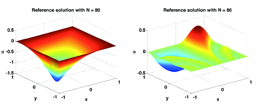
Fig. 1: The truth approximations for diffusion (left) and anisotropic wavespeed simulation (right) for $\mu_{1}=1$ and $\mu_{2}=0.5$ computed on a $81\times 81$ Chebyshev grid.

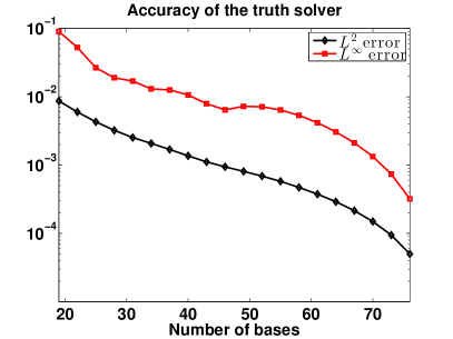
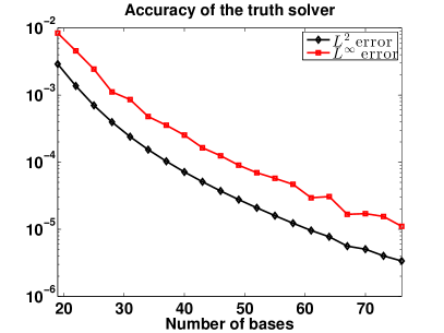
Fig. 2: The accuracy of truth approximations for diffusion (left) and anisotropic wavespeed simulation (right) for $\mu_{1}=1$ and $\mu_{2}=0.5$ with reference solution being computed on a $81\times 81$ Chebyshev grid.

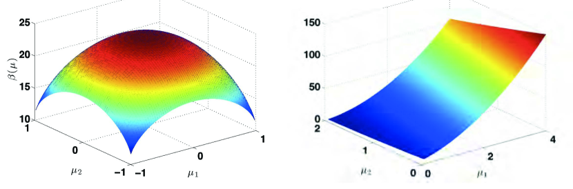
Fig. 3: The eigenvalues for the diffusion problem (left) and Anisotropic Wavespeed Simulation (right).

Before we begin with the reduced basis solver, we must quantify the accuracy of the fine-domain solver, which produces the truth approximations. Reference solutions computed by Chebyshev collocation method on a $81\times 81$ grid for $\mu_{1}=1$ and $\mu_{2}=0.5$ are plotted in Figure 1. We also compute the truth solutions on a ${\mathcal{N}}_{x}\times{\mathcal{N}}_{x}$ grid for ${\mathcal{N}}_{x}$ changing from $20$ to $77$ and evaluate the $L^{2}$ and $L^{\infty}$ errors. Exponential convergence of the truth approximation with respect to ${\mathcal{N}}$ is shown by Figure 2 as expected.

In the greedy algorithm, we required a lower bound on the eigenvalue of the operator. For the purposes of this work, we simply calculate the smallest eigenvalue for each $\mu\in\Xi$ and use it as the lower bound $\beta_{LB}(\mu)$. That is, the error estimator for the reduced basis solution $u_{\mu}^{(i)}$ based on a reduced basis set $\{u^{\mathcal{N}}_{\mu^{1}},\dots,u^{\mathcal{N}}_{\mu^{i}}\}$ is given by

$$\Delta_{i}(\mu)=\frac{\lVert{{\mathbf{f}}^{\mathcal{N}}-\mathbb{L}_{\mathcal{N}}(\mu)u_{\mu}^{(i)}}\rVert_{\ell^{2}}}{{\sqrt{\beta(\mu)}}}.$$

There are more efficient ways [12, 6, 11]. However, algorithm design and implementation of how to efficiently calculate $\beta_{LB}(\mu)$ is not an emphasis of this paper. Instead, we are concentrating on the design of the overall reduced basis method in the collocation framework. The eigenvalues $\beta(\mu)$ are plotted in Figure 3 for the two test problems. The first problem becomes close to being degenerate at the four corners of the parameter domain.

4.2 Results of the reduced solver: Anisotropic wavespeed simulation

In this section, we present the results of the two reduced collocation methods applied to the anisotropic wavespeed simulation.

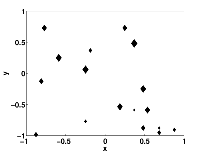
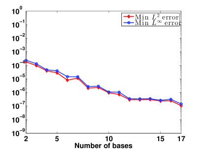
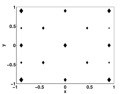
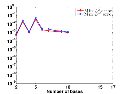
Fig. 4: Top: The reduced collocation points selected by the ERCM for Anisotropic wavespeed simulation, and the corresponding convergence plot. Bottom: The result of a (pre-determined) coarse Chebyshev grid was used.

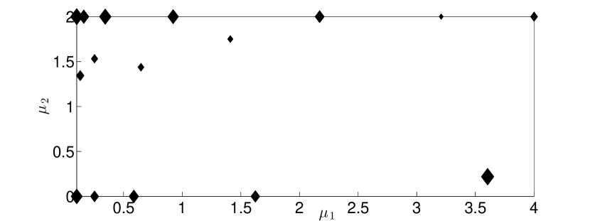
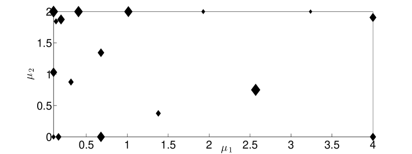
Fig. 5: The parameters picked by the greedy algorithm for pre-computation for the anisotropic wavespeed simulation. Top: Least Squares approach, bottom: Empirical Reduced Collocation Method.

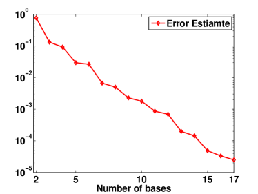
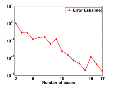
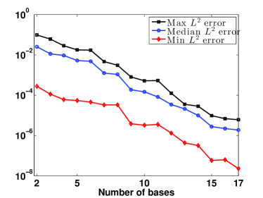
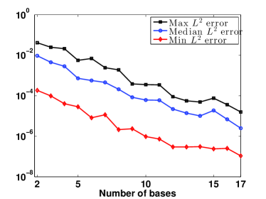
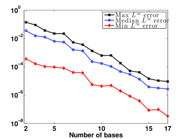
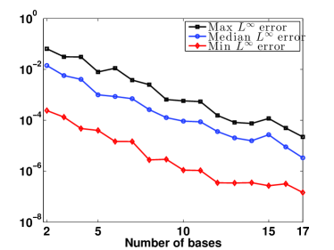
Fig. 6: History of convergence for the error estimate (top), the $L^{2}$ error (middle) and the $L^{\infty}$ error (bottom)of the RBM solutions for the anisotropic wavespeed simulation. On the left are for the least squares reduced collocation method, and the empirical reduced collocation results are on the right.

We first perform the offline pre-computation of the reduced basis and collocation points. The $17$ parameter values are chosen from $\Xi$ by Algorithms 1 and 2 are shown in Figure 5, with larger marker indicating the earlier that parameter picked. The reduced set of collocation points $C_{R}^{N}$ for ERCM is shown in Figure 4 (top left). $C_{R}^{i}$ contains the $i$ points in the computational domain $\Omega=[-1,1]^{2}$ corresponding to the $i$ largest markers.

Next, we solve for the reduced basis solution for a randomly selected set of $2,097$ parameter values in ${\mathcal{D}}$ and compute the maximum, median, and minimum errors for each selected value between the reduced solution and the truth approximations. These, together with the maximum of the error estimate are plotted in Figure 6. We clearly see exponential convergence in all cases by both methods. We compare Figure 2 and Figure 6 to draw the following remarkable conclusion: In the worst case scenario, using the empirical reduced collocation method on a $16=4\times 4$ grid can produce solution having comparable accuracy of the truth approximation on a grid $50\times 50$. We also see that, on average, the two proposed algorithms have similar accuracy. But, over a wide range of parameter values, the least squares approach seems to be more stable (the errors have smaller variance). Moreover, we show in Figure 4 how the choice of the reduced set of collocation points $C_{R}^{N}$ affects the accuracy of the reduced collocation method: our proposed method generates the reduced grid on the top left. The best case scenario for a randomly selected set of $2,097$ parameter values are shown on the top right. On the other hand, if we naively use a coarse Chebyshev grid as the $C_{R}^{N}$ (shown bottom left), the best case convergence plot is on the bottom right: the approximation is very bad with the system becoming numerically singular for $N>10$.

4.3 Results of the reduced solver: Diffusion

We set ${\mathcal{D}}=[-0.99,0.99]^{2}$, apply the empirical and least squares reduced collocation methods to the diffusion problem and present the results in this section.

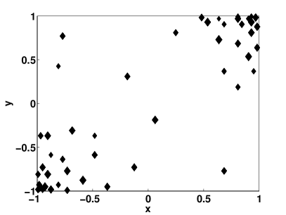
Fig. 7: The reduced collocation points selected by the ECM for diffusion problem.

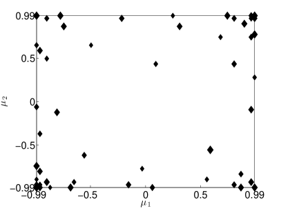
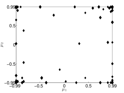
Fig. 8: The parameter values picked by the greedy algorithm for the diffusion equation. Left: Least squares. Right: reduced collocation.

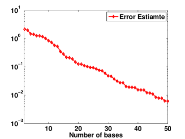
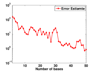
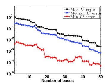
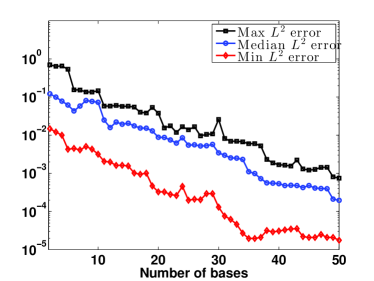
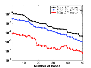
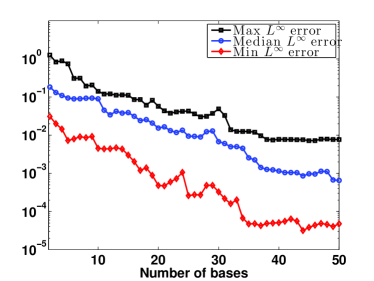
Fig. 9: History of convergence for the error estimate (top), the $\ell^{2}$ error (middle) and the $L^{\infty}$ error (bottom)of the RBM solutions for the diffusion problem. On the left are for the least squares approach, and the reduced collocation results are on the right.

We pick $50$ parameter values in ${\mathcal{D}}$ according to the greedy algorithm. The result is in Figure 8 with larger marker indicating the earlier it is picked. Correspondingly, the $50$ points in $\Omega$ determined by the ERCM for empirical reduced collocation are shown in Figure 7.

Next, we solve for the RB solutions for randomly selected set of $1,057$ parameter values and compute the maximum of the errors for all selected between the reduced solution and the truth approximations. These, together with the maximum of the error estimate are plotted in Figure 9. We clearly see exponential convergence in all cases for both methods.

4.4 Computation time of the reduced solver

In this section, we present statistics of the computation time for the reduced collocation methods. We present in Table 1 the offline and online computational time. We normalize the time with respect to that for solving truth approximation once. We see that the algorithm achieves savings of three orders of magnitude. From these examples, it seems that the empirical collocation approach is a little more efficient than the least-squares approach.

Method	Offline time	Online time for $u_{\mu}^{(N)}$	Time for $u_{\mu}^{\mathcal{N}}$
Anisotropic LSRCM	$1.029\,\times\,10^{3}$	$2.18\,\times 10^{-4}$	$1$
Anisotropic ERCM	$0.996\,\times 10^{3}$	$2.62\,\times 10^{-4}$	$1$
Diffusion LSRCM	$8.265\,\times 10^{3}$	$9.71\,\times 10^{-4}$	$1$
Diffusion ERCM	$7.730\,\times 10^{3}$	$10.69\,\times 10^{-4}$	$1$

Table 1: Computation times of the methods for the two test problems.

5 Concluding Remarks

In this paper, we propose the first reduced basis method for the collocation framework. Two rather different approaches have been proposed and tested. They are both Galerkin-free but produce the same fast exponential convergence and speedup as for the traditional Galerkin approach. In future work, we will examine the accuracy and efficiency of our proposed methods for non-affine and nonlinear problems. We also plan to study and tailor successive constraint method, currently used for computation of the lower bound for the eigenvalues in the Galerkin setting [12, 6, 11], for the collocation setting. It is also very interesting to apply the methods to more general collocation methods and to perform a detailed numerical comparison between the Galerkin approach and the collocation approaches introduced in this paper.

References

- [1] http://www.faculty.umassd.edu/yanlai.chen/
- [2] B. O. Almroth, P. Stern, and F. A. Brogan. Automatic choice of global shape functions in structural analysis. AIAA Journal, 16:525–528, May 1978.
- [3] M. Barrault, N. C. Nguyen, Y. Maday, and A. T. Patera. An “empirical interpolation” method: Application to efficient reduced-basis discretization of partial differential equations. C. R. Acad. Sci. Paris, Série I, 339:667–672, 2004.
- [4] P. Binev, A. Cohen, W. Dahmen, R. Devore, G. Petrova, and P. Wojtaszczyk. Convergence rates for greedy algorithms in reduced basis methods. SIAM J. MATH. ANAL, pages 1457–1472, 2011.
- [5] A. Buffa, Y. Maday, A. T. Patera, C. Prud’homme, and G. Turinici. A priori convergence of the greedy algorithm for the parametrized reduced basis. ESAIM-Math. Model. Numer. Anal., 2011. Special Issue in honor of David Gottlieb.
- [6] Y. Chen, J. S. Hesthaven, Y. Maday, and J. Rodríguez. A monotonic evaluation of lower bounds for inf-sup stability constants in the frame of reduced basis approximations. C. R. Acad. Sci. Paris, Ser. I, 346:1295–1300, 2008.
- [7] Y. Chen, J. S. Hesthaven, Y. Maday, and J. Rodríguez. Certified reduced basis methods and output bounds for the harmonic Maxwell’s equations. Siam J. Sci. Comput., 32(2):970–996, 2010.
- [8] Y. Chen, J. S. Hesthaven, Y. Maday, J. Rodríguez, and X. Zhu. Certified reduced basis method for electromagnetic scattering and radar cross section estimation. CMAME, 233:92–108, 2012.
- [9] M. A. Grepl, Y. Maday, N. C. Nguyen, and A. T. Patera. Efficient reduced-basis treatment of nonaffine and nonlinear partial differential equations. Mathematical Modelling and Numerical Analysis, 41(3):575–605, 2007.
- [10] J. S. Hesthaven, S. Gottlieb, and D. Gottlieb. Spectral methods for time-dependent problems, volume 21 of Cambridge Monographs on Applied and Computational Mathematics. Cambridge University Press, Cambridge, 2007.
- [11] D.B.P. Huynh, D.J. Knezevic, Y. Chen, J.S. Hesthaven, and A.T. Patera. A natural-norm successive constraint method for inf-sup lower bounds. CMAME, 199:1963–1975, 2010.
- [12] D.B.P. Huynh, G. Rozza, S. Sen, and A.T. Patera. A successive constraint linear optimization method for lower bounds of parametric coercivity and inf-sup stability constants. C. R. Acad. Sci. Paris, Srie I., 345:473 – 478, 2007.
- [13] Y. Maday, A. T. Patera, and G. Turinici. A priori convergence theory for reduced-basis approximations of single-parameter elliptic partial differential equations. J. Sci. Comput., 17:437–446, 2002.
- [14] D.A. Nagy. Modal representation of geometrically nonlinear behaviour by the finite element method. Computers and Structures, 10:683–688, 1979.
- [15] N. C. Nguyen, A. T. Patera, and J. Peraire. A ‘best points’ interpolation method for efficient approximation of parametrized functions. Internat. J. Numer. Methods Engrg., 73(4):521–543, 2008.
- [16] A. K. Noor and J. M. Peters. Reduced basis technique for nonlinear analysis of structures. AIAA Journal, 18(4):455–462, April 1980.
- [17] J. Pomplun and F. Schmidt. Accelerated a posteriori error estimation for the reduced basis method with application to 3D electromagnetic scattering problems. SIAM J. Sci. Comput., 32(2):498–520, 2010.
- [18] C. Prud’homme, D. Rovas, K. Veroy, Y. Maday, A. T. Patera, and G. Turinici. Reliable real-time solution of parametrized partial differential equations: Reduced-basis output bound methods. Journal of Fluids Engineering, 124(1):70–80, March 2002.
- [19] G. Rozza, D.B.P. Huynh, and A.T. Patera. Reduced basis approximation and a posteriori error estimation for affinely parametrized elliptic coercive partial differential equations: Application to transport and continuum mechanics. Arch Comput Methods Eng, 15(3):229–275, 2008.
- [20] J. Shen and T. Tang. Spectral and high-order methods with applications, volume 3 of Mathematics Monograph Series. Science Press Beijing, Beijing, 2006.
- [21] L. N. Trefethen. Spectral methods in MATLAB, volume 10 of Software, Environments, and Tools. Society for Industrial and Applied Mathematics (SIAM), Philadelphia, PA, 2000.