An order parameter for symmetry-protected phases in one dimension

Abstract

We introduce an order parameter for symmetry-protected phases in one dimension which allows to directly identify those phases. The order parameter consists of string-like operators and swaps, but differs from conventional string order operators in that it only depends on the symmetry but not on the state. We verify our framework through numerical simulations for the $\mathrm{SO}(3)$ invariant spin-$1$ bilinear-biquadratic model which exhibits a dimerized and a Haldane phase, and find that the order parameter not only works very well for the dimerized and the Haldane phase, but it also returns a distinct signature for gapless phases. Finally, we discuss possible ways to measure the order parameter in experiments with cold atoms.

Symmetries play an essential role almost everywhere in physics. A prominent example is Landau’s theory of phases: Different phases are classified by whether the state of the system obeys or breaks the symmetries of the Hamiltonian. In turn, this gives rise to local order parameters which can be measured to determine which phase a system is in. This picture has recently been challenged by the discovery of topologically ordered phases: They are not associated to the breaking of any local symmetry, and therefore there is no local order parameter which can be used to detect topological phases.

Topological order occurs only in two and higher dimensions, since one-dimensional gapped spin systems exhibit only a single phase. However, the situation in one dimension changes if we impose symmetries—they do not only give rise to Landau-type phases which are distinguished by local order parameters, but also to distinct symmetry-protected phases which cannot be distinguished by any local order parameter (and might thus be called topological), yet which are protected (i.e., separated) by the presence of the symmetry. The most prominent example for a non-trivial symmetry protected phase is the Haldane phase, which contains the spin-$1$ AKLT model and likely the spin-$1$ Heisenberg model and which is e.g. protected by $\mathrm{SO}(3)$ symmetry pollmann:1d-sym-protection-prb . More recently, it has been realized that these phases differ by the way in which the symmetry acts across blocks of the system, i.e., on the entanglement between blocks. This can be understood in a particularly natural way in the framework of Matrix Product States (MPS), which provide the appropriate framework for the description of gapped one-dimensional systems, and which allow to directly access the entanglement between blocks pollmann:1d-sym-protection-prb ; chen:1d-phases-rg ; schuch:mps-phases . In particular, it has been found that the action of the symmetry on the entanglement between blocks, and thus the different symmetry protected phases, are distinguished by the inequivalent projective representations of the symmetry group, such as integer and half-integer spin representations in the case of the rotation group pollmann:1d-sym-protection-prb ; chen:1d-phases-rg .

Symmetry protected phases such as the spin-$1$ AKLT chain do not exhibit long-range order, this is, non-decaying correlations between distant sites, which could otherwise replace local order parameters. However, they do exhibit what is known as string order nijs:string-order ; kennedy:string-order : Measuring a string of identical operators with distinct endpoints gives correlations which do not depend on the length of the string, despite the absence of conventional long-range order. This might suggest that string order parameters can be used to distinguish different symmetry-protected phases. However, the presence of string order is rather a signature of the symmetry itself than of the phase of the system under that symmetry, and string order parameters need to be tailored to the system under consideration; indeed, one can easily find examples of systems in different phases which are susceptible to the same string order parameter, and vice versa perez-garcia:stringorder-1d . Therefore, string order parameters are not well suited as order parameters for symmetry protected phases.

In this paper, we propose an order parameter which allows to distinguish symmetry-protected phases by directly measuring the way in which the physical symmetry acts on the entanglement between blocks. Unlike string order parameters, it is independent of the state under consideration and only depends on the symmetry itself. We demonstrate our approach for the $\mathrm{SO}(3)$ symmetry by numerically studying the spin–$1$ bilinear–biquadratic model (see, e.g., laeuchli:bilinear-biquadratic-nematic ), where we find that the order parameter, though defined for asymptotically large blocks, converges very well for small lengths. We also find that while the order parameter is designed to work for the gapped phases of the system, namely the trivial and the Haldane phase, it in fact also exhibits a distinct signature for the gapless critical and ferromagnetic phase of the model. Finally, we discuss how one could in principle experimentally implement a measurement of this order parameter, in particular with atoms in optical lattices.

Let us start by explaining the structure of one-dimensional gapped phases under symmetries; for simplicity, we will focus on systems with unique ground states. As such phases differ by their long-range properties, we first describe the structure of such states on large length scales, and in particular their renormalization group (RG) fixed points. Due to the absence of topological entanglement in one dimension, at the RG fixed point of 1D systems each site independently shares entanglement with its two adjacent sites. This is, the overall state is of the form

$$|\Psi\rangle=S^{\otimes N}|\lambda\rangle^{\otimes N}\ .$$ (1)

Here, $|\lambda\rangle=\sum\lambda_{i}|i,i\rangle$ is a “virtual” entangled state between adjacent sites with Schmidt spectrum $\lambda=(\lambda_{1},\dots,\lambda_{D})$, and $S$ is an isometry mapping the virtual entangled states into the physical system, acting jointly on the halves of two adjacent $|\lambda\rangle$ states, as depicted in Fig. 1. In the framework of Matrix Product States (MPS), which are obtained by replacing the isometry $S$ in Fig. 1 by an arbitrary linear map, and which form the appropriate class of states for the description of one-dimensional gapped quantum systems hastings:arealaw ; verstraete:faithfully ; schuch:mps-entropies , it can be proven rigorously that any ground state of a gapped 1D system converges exponentially to the fixed point of Eq. (1) verstraete:renorm-MPS ; thus, Eq. (1) can equally well be understood as an approximation to any gapped 1D system, where $S$ embeds the virtual entangled pairs into a block of $L$ physical sites each, with an accuracy exponential in $L$. (In this case, $S$ can be understood as the RG transformation on a block of length $L$).

Figure 1: Large-scale structure of 1D quantum states. The renormalization fixed point consists of virtual entangled pairs with Schmidt spectrum $\lambda$ between adjacent sites, which are mapped by an isometry $S$ onto the physical system. If $S$ maps onto $L$ sites of the original state, this ansatz approximates any ground state of a gapped Hamiltonian to an accuracy exponential in $L$.

Now consider a quantum system with an on-site linear symmetry $u_{g}$, $u_{g}^{\otimes N}|\Psi\rangle=|\Psi\rangle$, where $u_{g}$ is a representation of the symmetry group $G$, $u_{g}u_{h}=u_{gh}$. Under renormalization, the symmetry action transforms to the action $U_{g}$ on the renormalized sites. (In particular, if blocking $L$ sites, $U_{g}=u_{g}^{\otimes L}$.) In the representation of Eq. (1) and Fig. 1, this symmetry can be understood as an effective symmetry $\hat{U}_{g}=S^{-1}U_{g}S$ acting on the virtual entangled pairs. Note that $\hat{U}_{g}$ forms again a linear unitary representation of $G$, as $U_{g}$ commutes with $SS^{\dagger}$ schuch:mps-phases . It can be shown that the virtual action of the symmetry $\hat{U}_{g}$ always decomposes as $\hat{U}_{g}=V_{g}\otimes\bar{V}_{g}$, where $V_{g}$ and $\bar{V}_{g}$ act on the left and the right entangled state, respectively perez-garcia:stringorder-1d . Moreover, $\Lambda:=\sum\lambda_{i}|i\rangle\!\langle i|$ commutes with $\bar{V}_{g}$ schuch:mps-phases , so that $(\bar{V}_{g}\otimes V_{g})|\lambda\rangle=|\lambda\rangle$.

Since $\hat{U}_{g}=V_{g}\otimes\bar{V}_{g}$, and $\hat{U}_{g}\hat{U}_{h}=\hat{U}_{gh}$, it follows that $V_{g}$ forms a projective representation, $V_{g}V_{h}=e^{i\omega(g,h)}V_{gh}$. Here, $\omega(g,h)$ is a 2-cocycle, i.e., it satisfies $\omega(g,hk)+\omega(h,k)=\omega(g,h)+\omega(gh,k)\mathrm{\ mod\,}2\pi$. As $V_{g}$ is only defined up to its phase (and up to a similarity transform), we have a gauge degree of freedom $V_{g}\leftrightarrow e^{i\phi_{g}}V_{g}$ which induces an equivalence relation $\omega(g,h)\sim\omega(g,h)+\phi_{g}+\phi_{h}-\phi_{gh}\mathrm{\ mod\,}2\pi$ of $2$-cocycles, and thus equivalence classes of projective representations. These equivalence classes form a group isomorphic to the second cohomology group $\mathrm{H}^{2}(G,\mathrm{U}(1))$, and label the inequivalent projective representations of the symmetry group $G$. For the rotation group $\mathrm{SO(3)}$, e.g., the inequivalent projective representations are the integer and half-integer spin representations, respectively. It turns out that the equivalence class of the projective representation $V_{g}$, which describes the action of the symmetry on the virtual degrees of freedom, is exactly what labels different phases in the presence of symmetries chen:1d-phases-rg ; schuch:mps-phases .

Figure 2: Illustration of the measurement Eq. (2) used to determine phases under $\mathrm{SO}(3)$ symmetry (with shorthand $Z$ for $V_{z}$, etc.). By following the loops created by the operator and the entangled states, it can be easily checked that the diagram evaluates to $\mathcal{E}(\Psi)$, Eq. (3); note that operators traversed downwards have to be transposed.

In order to detect different symmetry protected phases, we therefore need a measurement which allows us to determine the equivalence class of the projective representation with which the symmetry acts on the entanglement between blocks. However, the problem is that while we know $U_{g}$, it is impossible to infer sufficient information about $V_{g}$ from it—to do so we would have to know the transformation $S$, which would require full tomography of the state . Fortunately, we do not need detailed knowledge of $V_{g}$, since we only want to know to which equivalence class of projective representations it belongs. For this purpose, it is sufficient to compute certain gauge invariant quantities which give access to the gauge invariant universal signature of $\omega(g,h)$: For instance, for $\mathrm{SO}(3)$ symmetry, one such quantity is $V_{z}V_{x}V_{z}^{\dagger}V_{x}^{\dagger}$, where $x,z\in\mathrm{SO(3)}$ denote $\pi$ rotations about the $x$ and the $z$ axis: It is $+\openone$ for integer spin representations and $-\openone$ for half-integer spin representations of $\mathrm{SO}(3)$, respectively, and does not depend on the gauge. (See Appendix A for other groups.) Thus, if we were able to measure such an invariant for a given state, we would be able to determine the symmetry protected phase the system is in. Different from determining $V_{g}$ itself, this invariant can be determined without any information about $S$, by measuring a suitable operator such as

$$\mathcal{E}(\Psi):=\langle\Psi|(U_{z}\otimes U_{z}\otimes\openone)\mathbb{F}_{13}(U_{x}\otimes U_{x}\otimes\openone)|\Psi\rangle\ ,$$ (2)

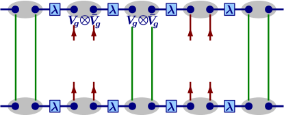
where $\mathbb{F}_{13}$ swaps the first and the third site. [Equivalently, $\mathcal{E}(\Psi)=\langle\Psi|\mathbb{F}_{13}U_{x}U_{y}U_{z}|\Psi\rangle$.] If one expresses this measurement diagrammatically using that $\hat{U}_{g}=V_{g}\otimes\bar{V}_{g}$, cf. Fig. 2, it is straightforward to check that

$$\mathcal{E}(\Psi)=\mathrm{tr}[V_{z}V_{x}V_{z}^{\dagger}V_{x}^{\dagger}\Lambda^{4}]\,\mathrm{tr}[\Lambda^{4}]\ ,$$ (3)

and its sign thus allows to determine the phase of $|\Psi\rangle$. (Recall that $\Lambda$ commutes with $V_{g}$.) Note that by omitting the $U$’s in Eq. (2), one can measure $\mathcal{N}(\Psi):=\mathrm{tr}[\Lambda^{4}]^{2}$, and that the ratio $\hat{\mathcal{E}}(\Psi):=\mathcal{E}(\Psi)/\mathcal{N}(\Psi)=\pm 1$ yields a normalized quantity which distinguishes the trivial from the Haldane phase. (See Appendix B for how to measure general gauge invariant quantities.)

The preceding discussion was concerned with renormalization fixed points, i.e., states of the form Eq. (1). However, we can evaluate the same quantity for an arbitrary quantum state, by replacing $U_{x}$ and $U_{z}$ by strings of local symmetry operators $u_{x}$ and $u_{z}$, i.e., $U_{g}=u_{g}^{\otimes L}$. For ground states of gapped Hamiltonians, we expect it to converge exponentially fast to the value at the renormalization fixed point; this can be proven rigorously in the framework of Matrix Product States, cf. Appendix C.

In order to test the applicability of the order parameter, we have performed numerical simulations for the spin-$1$ bilinear-biquadratic Heisenberg chain (cf., e.g., laeuchli:bilinear-biquadratic-nematic and references therein)

$$H(\theta)=\cos\theta\sum_{i}{\bm{S}}_{i}\cdot{\bm{S}}_{i+1}+\sin\theta\sum_{i}(\bm{S}_{i}\cdot\bm{S}_{i+1})^{2}\,.$$ (4)

This model is $\mathrm{SO}(3)$ invariant and exhibits both possible gapped phases under rotational symmetry: A dimerized phase for $-3\pi/4<\theta<-\pi/4$ (with integer spin representations $V_{g}$ and thus topologically trivial), and a Haldane phase for $-\pi/4<\theta<\pi/4$ (with half-integer representations $V_{g}$ and thus topologically non-trivial).

Figure 3: Order parameter $\mathcal{E}_{L}$ for the bilinear-biquadratic spin-$1$ model, Eq. (4), as a function of $\theta$, for different estimator lengths $L$. The inset shows the normalized order parameter $\hat{\mathcal{E}}_{L}$. Note that $-1/4\leq\mathcal{E}\leq 1$ from the minimal dimension of the corresponding representations. $\mathcal{E}=-1/4$ is attained at the ALKT point ($\theta/\pi\approx 0.1024$).

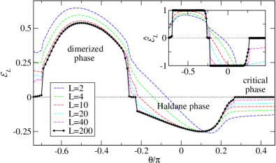
The simulations have been carried out using infinite Matrix Product States (iMPS) vidal:iTEBD with sites blocked in pairs, using the time-dependent variational principle haegeman:varprinciple-lattices . The results for the order parameter ${\mathcal{E}_{L}}$ as a function of $\theta/\pi$ are plotted in Fig. 3 for different length $L$ ($L$ refers to the length of a single block in Fig. 2), and for $D=32$; the inset shows the normalized $\hat{\mathcal{E}_{L}}$. We find that $\mathcal{E}_{L}$ converges quickly, with its sign correctly distinguishing the dimerized phase ($+1$) from the Haldane phase ($-1$). Deviations from this behavior can be observed at the phase transitions around $\theta=\pm\pi/4$, as well as in the dimerized phase close to $\theta=-3\pi/4$, a regime in which the possible existence of a “spin-nematic phase” is under ongoing debate (see, e.g., laeuchli:bilinear-biquadratic-nematic ). Simulations with different $D$ give similar results, except that the width of the transition regions between the phases decreases with increasing $D$.

A closer analysis of the data reveals that inside both phases, $\mathcal{E}_{L}$ converges exponentially with a length scale essentially equal to the correlation length (deviation below $2\%$). However, for many values of $\theta$ this behavior is only seen on intermediate length scales (typically up to $L\approx 30\dots 40$), while at larger scales, $\mathcal{E}_{L}$ tends to zero. This can be understood as follows: Finding the optimal MPS approximation with a given $D$ corresponds to keeping the $D$ largest values in the Schmidt spectrum $\lambda$ of the state. As $[\Lambda,V_{g}]=0$, the degeneracies in the Schmidt spectrum correspond to the irreps of $\mathrm{SO}(3)$ which appear in $V_{g}$. If the truncation does not respect these degeneracies (this depends on the ordering of the irreps in the Schmidt spectrum and thus on the point $\theta$ in the phase), the resulting iMPS will not any more be exactly $\mathrm{SO}(3)$ invariant, which causes $\mathcal{E}_{L}$ to converge to zero. For the data reported in Fig. 3 with $D=32$, we find perfect convergence for $\theta/\pi=-0.69\,\dots-0.63$ and $\theta/\pi=-0.22\dots{-0.10}$. In Fig. 4a, we compare the two cases for two adjacent points in the dimerized phase.

Figure 4: Convergence analysis. a) Normalized order parameter $\hat{\mathcal{E}}_{L}$ for $\theta/\pi=-0.62$ and $-0.63$. Initially, both converge to $1$ exponentially with similar exponent, but for $\theta/\pi=-0.62$, the convergence is not perfect as $D$ is incommensurate with the representation of the symmetry. b) Algebraic decay in the critical phase. After correcting for the exponential decay from the iMPS approximation and oscillations, we find that the estimator goes to zero algebraically. For the fit, we have only used $L$ with $\mathrm{mod}(L,3)\neq 0$.

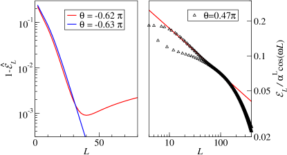
Beyond the dimerized and the Haldane phase, the bilinear-biquadratic model also exhibits two gapless phases. Firstly, a ferromagnetic phase for $\pi/2\!\leq\theta\leq 5\pi/4$ with product ground states $|\phi\rangle^{\otimes N}$; there, $\mathcal{E}_{L}=(\langle\phi|u_{x}|\phi\rangle\langle\phi|u_{y}|\phi\rangle\langle\phi|u_{z}|\phi\rangle)^{L}$ converges to zero exponentially in $L$. Secondly, there is a critical phase in the regime $\pi/4\leq\theta<\pi/2$ laeuchli:bilinear-biquadratic-nematic which we have included in our simulations, cf. Fig. 3. The results for this region should be taken with care, as MPS perform considerably worse in describing the ground states of critical systems, and in particular cannot exactly reproduce algebraically decaying correlations. Analyzing the behavior of the order parameter in the critical regime, we find a dominating exponential decay due to the fact that $D$ is incommensurate with the symmetry, which is superimposed with an oscillation due to the $2\pi/3$ periodicity of the critical phase laeuchli:bilinear-biquadratic-nematic , $\alpha^{L}\cos(\omega L)$. The parameters $\alpha$ and $\omega$ can be extracted from the MPS transfer operator, and we find that after correcting for these effects, $\hat{\mathcal{E}}_{L}/(\alpha^{L}\cos(\omega L))$ (plotted in Fig. 4b for $\theta=0.47$) exhibits an algebraic decay to zero, with an exponent which varies between $0.41$ and $0.44$ in the critical phase. The results on the exponent should be taken with particularly great care, as they depend on the choice of data points fitted, and the algebraic decay observed is in fact a sum of exponentials; yet, we believe that our results provide substantial evidence for an algebraically vanishing order parameter in the critical phase.

So far, we have shown that the order parameter ${\cal E}(\Psi)$ can be used as a theoretical tool to determine the phases of 1D spin chains. Now we will show that, at least in principle, it can also be experimentally determined by performing few measurements (without the need of carrying out a full tomography). The main idea is to use an ancillary particle which controls whether the unitary and swapping operations appearing in Eq. (2) are applied or not, and then perform a measurement on that particle. Let us assume that the ancilla is a qubit, initially prepared in the state $(|0\rangle+|1\rangle)/\sqrt{2}$. Then, the ancilla interacts successively with particles in region 1 and 2, 1 and 3, and then again 1 and 2, such that if it is in state $|1\rangle$, the unitary operator appearing in Eq. (2) is applied, and otherwise just the identity operator. At the end of the process, one measures the Pauli operator $\sigma_{x}$ on the ancilla, whose expectation value conincides with ${\cal E}(\Psi)$.

The techniques required to carry out the above procedure are very sophisticated, and we do not expect that they can be performed in most of the experimentally relevant situations (beside atomic physics experiments, where individual addressing and full control over the atomic interactions may be gained in the near future greiner:atomaddressing ; bloch:atomaddressing ; bloch:stringorder ). In any case, here we give an alternative method to detect the phase which may be slightly simpler to implement in the particular setup of atoms in optical lattices. The main idea is to use two copies of the spin chain, as it is usual in that setup (for instance, with the help of superlattices lewenstein:reviewlattices ). Then, one would like to determine

$${\cal E}^{(2)}(\Psi):= \langle\Psi|_{A}\langle\Psi|_{B}(\mathbb{F}_{1A,1B}\otimes\mathbb{F}_{3A,3B})\,\times$$ (5)

$$\quad(U_{z}^{1,A}\otimes U_{z}^{1,B}\otimes U_{x}^{2,A}\otimes U_{x}^{2,B})|\Psi\rangle_{A}|\Psi\rangle_{B}\ .$$

Here, $A$ and $B$ refer to the first and second copy of the chain, and 1, 2, and 3 to three neighboring regions each containing a sufficiently large number of spins. One can easily convince oneself that ${\cal E}^{(2)}$ contains the same information as ${\cal E}$. The advantage of this measurement is that the swap only occurs between particles in two chains which are adjacent to each other. In practice, the ancilla could consist of a different atomic species (see Aguado:ancillaatoms ), so that it can be transported independently of the spin chains. As explained in that reference, one could use this ancilla to apply the conditional unitary operators sequentially to the spin chains. Additionally, the swapping operator can be generated by letting the ancilla control the pairwise interaction among the neighboring spins of the first and second chain in regions 1 and 3, corresponding to a Hamiltonian $H=\sum(h_{i}+h_{i}^{2})$, where $h_{i}={\bm{S}}_{i,A}\cdot{\bm{S}}_{i,B}$, for a time $t=\pi/2$. We would like to emphasize that this procedure may be very difficult in practice, but it still shows that in principle one can measure the order parameter.

To conclude, in this paper we have introduced an order parameter for symmetry protected phases in one dimension. We have illustrated our construction for $\mathrm{SO(3)}$ symmetry, where we have verified our predicitions numerically for the spin-$1$ bilinear-biquadratic model. We found that the order parameter allows to faithfully determine which gapped phase the system is in; moreover, we found that (somewhat surprisingly) it also returns a distinct signature for the gapless phases of the model.

Similar order parameters can be constructed for symmetry protected gapped phases with partial symmetry breaking schuch:mps-phases , by first using conventional local order parameters to detect which symmetries are broken, and subsequently measuring order parameters such as the one presented to detect the topological phase protected by the remaining unbroken symmetries. An interesting open question is whether our method to identify equivalence classes of $2$-cocycles, corresponding to elements in $\mathrm{H}^{2}(G,\mathrm{U}(1))$, can be modified to distinguish symmetry protected phases in two dimensions, which are labelled by equivalence classes of $3$-cocycles and correspondingly the third cohomology group $\mathrm{H}^{3}(G,\mathrm{U}(1))$. Finally, as the endpoints of string operators can be interpreted as quasi-particles, it would be interesting to understand whether our order parameter can be effectively understood as extracting information about the quasi-particle braiding properties.

Acknowledgments.—We thank J. de Boer and F. Verstraete for helpful comments. Parts of this work were carried out at the Perimeter Institute in Waterloo, Canada, and the Centro de Ciencias Pedro Pascual in Benasque, Spain. This work has been supported by the Alexander von Humboldt Foundation, the Caltech Institute for Quantum Information and Matter (an NSF Physics Frontiers Center with support of the Gordon and Betty Moore Foundation), the NSF Grant No. PHY-0803371, the EU grants QUEVADIS and QUERG, the Spanish projects QUITEMAD and MTM2011-26912, the FWF SFB grants FoQuS and ViCoM, and the DFG-Forschergruppe 635.

Appendix A Appendix A: Distinguishing inequivalent projective representations

As we show in Appendix B, we can measure any gauge-invariant quantity of the form

$$\mathrm{tr}[\tilde{V}_{g}\tilde{V}_{h}\dots]\,\times\,\mathrm{tr}[\tilde{V}_{k}\tilde{V}_{\ell}\dots]\,\times\cdots\ ,$$

where $\tilde{V}_{g}$ is either $V_{g}\Lambda$ or $V_{g}^{\dagger}\Lambda$, and for each $g$, $V_{g}$ and $V_{g}^{\dagger}$ appear an equal number of times. Since $[V_{g},\Lambda]=0$, we can (and will) omit the $\Lambda$’s in the following. As we are interested in gauge-invariant observables, the product of the group elements in each trace must be equal to the identity, and it follows that it is sufficient to consider a single trace. (Note that this is all we can measure, since $V_{g}$ is only defined up to a phase and similarity transform, $V_{g}\leftrightarrow e^{i\phi_{g}}X_{g}V_{g}X_{g}^{-1}$.)

Let us now discuss some cases beyond $\mathrm{SO}(3)$ in which we can identify the equivalence class of the projective representation by such a measurement. Most importantly, this holds for any special orthogonal group $\mathrm{SO}(N)$, $N\geq 3$, all of which have a two-fold covering by the corresponding spin group $\mathrm{Spin}(N)$, and correspondingly $\mathrm{H}^{2}(\mathrm{SO}(N),\mathrm{U}(1))=\mathbb{Z}_{2}$. As for $\mathrm{SO}(3)$, $V_{x}V_{z}V_{x}^{\dagger}V_{z}^{\dagger}=\pm\openone$, with $x$ and $z$ $\pi$-rotations about two orthogonal axes, will allow to identify the equivalence class of $V_{g}$. (This can e.g. be understood by considering projective representations of the subgroup $\mathbb{Z}_{2}\times\mathbb{Z}_{2}$ generated by $x$ and $z$.) Furthermore, the same result holds for any subgroup of $\mathrm{SO}(N)$ containing the group elements which appear in the measurement, such as $x$ and $z$. We expect similar measurements to exist for other finite groups.

Appendix B Appendix B: Measuring general gauge-invariant quantities

Figure 5: Elementary gadget used to construct arbitrary gauge invariant measurements. It has two input sites and two output sites (each consisting of a left and a right subsystem), which can be arbitrarily wired together by swapping sites.

In this appendix, we show how to measure an arbitary gauge invariant quantity of the form

$$\mathrm{tr}[\tilde{V}_{g}\tilde{V}_{h}\dots]\,\times\,\mathrm{tr}[\tilde{V}_{k}\tilde{V}_{\ell}\dots]\,\times\cdots\ ,$$ (6)

where $\tilde{V}_{g}$ is either $V_{g}\Lambda$ or $V_{g}^{\dagger}\Lambda$, the product in each trace is proportional to the identity (allowing us to disregard $\Lambda$’s) and for each $g$, $V_{g}$ and $V_{g}^{\dagger}$ appear an equal number of times, ensuring gauge invariance. The measurement is implemented by concatenating the elementary “gadgets” of the form of Fig. 5, which we think of as objects with two “inputs” (the top row) and two “outputs” (the bottom row); the outputs are related to the inputs by multiplication with $(V_{g}\Lambda)\otimes\Lambda$ and $(V_{g}^{\dagger}\Lambda)\otimes\Lambda$, respectively. It is now easy to see that arranging the gadgets for all required $V_{g}$ one after another, and appropriately connecting inputs and outputs (corresponding to a permutation of the input/output sites), the observable Eq. (6) can be measured.

Appendix C Appendix C: Convergence to RG fixed point

Let us show that for MPS, $\mathcal{E}_{L}$ converges exponentially to the value at the RG fixed point. To this end, let $A^{i}$ be the MPS matrices, implicitly defined via $S=\sum(A^{i})_{\alpha\beta}|i\rangle\langle\alpha,\beta|$, where the gauge $A^{i}\leftrightarrow XA^{i}X^{-1}$ is chosen according to Ref. perez-garcia:mps-reps . Define the transfer operators $\mathbb{E}=\sum\bar{A}^{i}\otimes A^{i}$ and

$$\mathbb{E}_{g}=\sum(u_{g})_{ij}\bar{A}^{i}\otimes A^{j}=(\openone\otimes V_{g})\mathbb{E}(\openone\otimes V_{g})^{\dagger}\ .$$

With $\mathbb{T}=\mathbb{E}^{L}$ and $\mathbb{T}_{g}=\mathbb{E}_{g}^{L}$, we have that

$$\mathcal{E}_{L}(\psi)=\sum\mathbb{L}^{ii^{\prime}}(\mathbb{T}_{x})_{ik^{\prime}}^{j\ell^{\prime}}(\mathbb{T}_{xz})_{jj^{\prime}}^{kk^{\prime}}(\mathbb{T}_{z})_{ki^{\prime}}^{\ell j^{\prime}}\mathbb{R}_{\ell\ell^{\prime}}$$

where lower (upper) indices denote the left (right) indices of the transfer operators, and $\mathbb{L}=\Lambda$, $\mathbb{R}=\openone$ are the unique left and right fixed points of $\mathbb{T}$ perez-garcia:mps-reps . The normalization $\mathcal{N}_{L}(\psi)$ is obtained by replacing all $\mathbb{T}_{g}$ by $\mathbb{T}$. As $\mathbb{T}_{g}=(\openone\otimes V_{g})\mathbb{T}(\openone\otimes V_{g})^{\dagger}$, and $\mathbb{T}$ converges to its fixed point $|\openone\rangle\langle\Lambda|$ exponentially in $L$, exponential convergence of $\mathcal{E}_{L}$ and $\mathcal{N}_{L}$ follows. Note that the length scale of convergence is given by the gap of $\mathbb{T}$ and is thus equal to the correlation length.

References

- (1) F. Pollmann, A. M. Turner, E. Berg, and M. Oshikawa, Phys. Rev. B 81, 064439 (2010), arXiv:0910.1811.
- (2) X. Chen, Z. Gu, and X. Wen, Phys. Rev. B 83, 035107 (2011), arXiv:1008.3745.
- (3) N. Schuch, D. Perez-Garcia, and I. Cirac, Phys. Rev. B 84, 165139 (2011), arXiv:1010.3732.
- (4) M. den Nijs and K. Rommelse, Phys. Rev. B 40, 4709 (1989).
- (5) T. Kennedy and H. Tasaki, Phys. Rev. B 45, 304 (1992).
- (6) D. Perez-Garcia, M. Wolf, M. Sanz, F. Verstraete, and J. Cirac, Phys. Rev. Lett. 100, 167202 (2008), arXiv:0802.0447.
- (7) A. Läuchli, G. Schmid, and S. Trebst, Phys. Rev. B74, 144426 (2006), cond-mat/0607173.
- (8) M. Hastings, J. Stat. Mech. , P08024 (2007), arXiv:0705.2024.
- (9) F. Verstraete and J. I. Cirac, Phys. Rev. B 73, 094423 (2006), cond-mat/0505140.
- (10) N. Schuch, M. M. Wolf, F. Verstraete, and J. I. Cirac, Phys. Rev. Lett. 100, 30504 (2008), arXiv:0705.0292.
- (11) F. Verstraete, J. Cirac, J. Latorre, E. Rico, and M. Wolf, Phys. Rev. Lett. 94, 140601 (2005), quant-ph/0410227.
- (12) E.g., if for contains both the spin- and spin- representation, could act either as or as , depending on .
- (13) G. Vidal, Phys. Rev. Lett. 98, 070201 (2007), cond-mat/0605597.
- (14) J. Haegeman et al., Phys. Rev. Lett. 107, 070601 (2011), arXiv:1103.0936.
- (15) W. S. Bakr, J. I. Gillen, A. Peng, S. Foelling, and M. Greiner, Nature 462, 74 (2009), arXiv:0908.0174.
- (16) J. F. Sherson et al., Nature 467, 68 (2010), arXiv:1006.3799.
- (17) M. Endres et al., Science 334, 200 (2011), arXiv:1108.3317.
- (18) M. Lewenstein et al., Advances in Physics 56, 243 (2007), cond-mat/0606771.
- (19) M. Aguado, G. K. Brennen, F. Verstraete, and J. I. Cirac, Phys. Rev. Lett. 101, 260501 (2008), arXiv:0802.3163.
- (20) D. Perez-Garcia, F. Verstraete, M. M. Wolf, and J. I. Cirac, Quant. Inf. Comput. 7, 401 (2007), quant-ph/0608197.