Studying the asymmetry of the GC population of NGC 4261

Abstract

We present an analysis of the Globular Cluster (GC) population of the elliptical galaxy NGC 4261 based on $HST$ WFPC2 data in the $B$, $V$ and $I$ bands. We study the spatial distribution of the GCs in order to probe the anisotropy in the azimuthal distribution of the discrete X-ray sources in the galaxy revealed by Chandra images (Zezas et al., 2003). The luminosity function of our GC sample (complete at the 90% level for $m_{{}_{V}}$ = 23.8 mag) peaks at $m_{{}_{V}}$ = 25.1${}_{-0.6}^{+1.0}$ mag, which corresponds to a distance consistent with previous measurements. The colour distribution can be interpreted as being the superposition of a blue and red GC component with average colours $V-I$ = 1.01${}_{-0.06}^{+0.06}$ mag and 1.27${}_{-0.08}^{+0.06}$ mag, respectively. This is consistent with a bimodal colour distribution typical of elliptical galaxies. The red GC’s radial profile is steeper than that of the galaxy surface brightness, while the profile of the blue subpopulation looks more consistent with it. The most striking finding is the significant asymmetry in the azimuthal distribution of the GC population about a NE-SW direction. The lack of any obvious feature in the morphology of the galaxy suggests that the asymmetry could be the result of an interaction or a merger.

1 Introduction

Elliptical galaxies are spheroidal systems which are expected to present a highly uniform spatial distribution of starlight and Globular Cluster (GC) sources. Nevertheless, optical images show that several elliptical galaxies exhibit structures such as shells, ripples, arcs, tidal tails and other asymmetric features (e.g. Schweizer & Seitzer, 1992). One of the most popular scenarios for elliptical galaxy formation suggests that these features are the result of major mergers. Numerical simulations (e.g. Toomre & Toomre, 1972; Barnes, 1988) show indeed that such mergers are characterized by peculiar remnant structures of this type. Minor merging events and interactions can subsequently disturb further the galaxy morphology.

Merger events and galaxy encounters affect the spatial distribution of the stellar population as well as that of the GC population. Schweizer & Seitzer (1992) discovered significant structure in the starlight of several elliptical galaxies, and disturbed orbits are found in NGC1404 and NGC1399, probably due to a dynamical interaction between the two galaxies (Napolitano, Arnaboldi, & Capaccioli 2002; Bekki et al. 2003). The amplitude of the deviation from the isotropy in either the stellar or GC populations in elliptical systems obviously depends on the time lapsed since the merging/interaction event, as well as on the nature of the event itself, and so may be used to explore the elliptical galaxy’s formation history.

1.1 The Case of NGC4261

NGC 4261 is a nearby (29.4$\pm$2.6 Mpc; Jensen et al. 2003) early-type galaxy in the Virgo W cloud (Garcia, 1993; Nolthenius, 1993). It is a well-studied object thanks to many interesting features: it has an active nucleus hosting a supermassive black hole (4.9$\pm$1.0)$\times$10⁸M_☉ (Ferrarese, Ford, & Jaffe, 1996), it hosts the radio source 3C 270, whose prominent radio jets (Birkinshaw & Davies, 1985) are associated with X-ray emission close to the nucleus (Worrall et al., 2010). It shows a 20″dust lane along the north-south axis (Martel et al., 2000) and has an impressive nuclear dust disk, discovered with HST WFPC2 (Jaffe et al., 1996).

Apart from the “boxy“ isophotes (e.g. Nieto & Bender, 1989) and weak evidence for a tidal arm in the NW direction (Tal et al., 2009), this galaxy does not show any definite story of recent interaction such as shells, ripples, rings, resulting in a low fine structure parameter ($\Sigma$=1.0; Schweizer & Seitzer, 1992). Therefore, despite being the most massive object in a poor group of galaxies (Davis et al., 1995), we can claim that NGC 4261 does not show evidence of recent gravitational interaction.

Given the undisturbed starlight distribution of NGC 4261, the discrete X-ray sources (i.e. X-ray binaries) would be expected to be distributed uniformly. However, Chandra data pointed to an interesting anisotropy in their azimuthal distribution, and more precisely to an excess between P.A.=140^∘ and P.A.=190^∘ (Zezas et al., 2003). Giordano et al. (2005) associated 50% of these sources with GCs identified in archival optical images and suggested that the Chandra sources are accreting Low Mass X-ray Binaries (LMXBs). This result suggests a non-uniform distribution of the GC population.

In order to investigate this hypothesis, we requested deep HST WFPC2 data (proposal ID 11339; PI: Zezas, A - Table 1) to characterize the GC population of NGC 4261. In this paper we present a study of the radial and azimuthal distributions of the blue (metal poor) and red (metal rich) GC subpopulations. We assess the extent of the asymmetry and discuss its origin in the context of a galaxy interaction. In a following paper (Bonfini et al., in preparation), we will extend the analysis to the LMXB population using the new deep Chandra pointing. In particular, by probing whether the LMXBs and GCs indeed have similar spatial distribution, we will add to the debate on whether GCs are the sole birthplaces of LMXBs (e.g. White, Sarazin, & Kulkarni, 2002), or field LMXBs form independently in situ (e.g. Kundu, Maccarone, & Zepf, 2007, and references therein), or, as suggested by the recent work of Kim et al. (2009), both formation processes contribute to the field LMXB population of elliptical galaxies.

The outline of the paper is as follows. In $\S$2 we describe the HST data reduction and source detection. In $\S$3 we report the criteria used to define GC candidates and we describe the procedure used to correct the Luminosity Function (LF) for incompleteness. In $\S$4 we study the Globular Cluster Luminosity Function (GCLF) and colour distribution. In $\S$5 we study the azimuthal and radial distributions of the GCs. In $\S$6 we discuss our results in the context of the recent interaction history of NGC 4261.

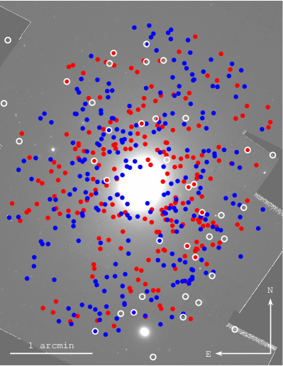
Figure 1: $I$ band mosaic. Blue and red markers represent the position of blue and red secure GCs down to the 75% completeness limit (sample and choice of completeness limit are defined in Section $\S$3 and $\S$5, respectively). These are the sources on which we performed the study of the spatial distribution. The white open circles represent the locations of X-ray sources in the source list of Giordano et al. 2005.

2 Optical Observations and Data Analysis

2.1 Data Reduction

HST WFPC2 data for NGC 4261 were obtained with the F450W, F606W and F814W filters (roughly corresponding to the B, V and I bands, respectively; see WFPC2 Instrument Handbook, Version 10.0, Table 3.1 ). The filters were chosen to provide the highest sensitivity while allowing us to distinguish the blue and red GC subpopulations.

In order to reject cosmic rays the observations were performed following a two point dither pattern with a 0.3 pixel offset. A total of 12 exposures of 400 s each were acquired in each filter in a 3$\times$2 grid. The pointings were planned in order to cover the $D_{25}$ (major diameter; 4′.07 de Vaucouleurs et al., 1991) area of the galaxy. The details of the observations are reported in Table 1.

Table 1: LOG OF THE OBSERVATIONS

Instrument	Filter	Number	Date	Exposure
		of		per Field
		Fields		(sec)
HST WFPC2	F450W ($B$)	6	2008 Jan 12	(2$\times$)400
			2008 Jan 13
HST WFPC2	F606W ($V$)	6	2007 Dec 26	(2$\times$)400
HST WFPC2	F814W ($I$)	6	2008 Jan 28	(2$\times$)400
			2008 Mar 10

Mosaics of the HST images were created with the following procedure. The task MultiDrizzle (within the PyRAF package, DITHER version 2.3) had been first used to produce the distortion corrected frames for each exposure. Then, the relative offsets between the fields were determined by comparing the coordinates of stars present in overlapping regions of these frames. The pointlike sources within each frame were detected using daofind, while the PyRAF tasks xyxymatch and geomap were used to calculate the offsets. Due to the small number of stars in the field of view, we could identify only 2-5 sources in common between each pair of fields, therefore in some cases we had to include some GCs as reference objects. The offset table created in this way was fed to MultiDrizzle in order to create the final version of the mosaic. The mosaics for the different filters were registered with respect to the $I$ band image. The final image was binned to the Wide Field Camera CCD pixel scale (WFC; nominally, 0.0996″/pixel).

Subsequently, we corrected for systematic astrometry errors by cross-correlating the HST coordinates of the 50 brightest objects (counts $>$ 4000) in the $I$ band mosaic (see $\S$2.2 for the source detection technique) against the coordinates of the 50 brightest Sloan Digital Sky Survey - Data Release 5 (SDSS DR5; Adelman-McCarthy et al., 2007) sources in the field. The SDSS catalogue provided a more reliable calibration since it is richer in astrometric reference stars than the HST field. We performed the astrometric correction using the WCSTOOLS imwcs, which produced a significant number of matches (11/50), allowing us to measure a negligible WCS offset of ($\Delta$RA,$\Delta$Dec) = (-0.02$\pm$0.10″,0.01$\pm$0.13″). The same WCS solution was then applied to the $B$ and $V$ band mosaics.

Figure 1 shows the final drizzled image for filter $I$, along with the location of the blue and red GCs of our secure sample down to the 75% completeness limit (the sample and choice of completeness limit are defined in $\S$3 and $\S$5, respectively). In the figure we also show the locations of the X-ray sources in the list of Giordano et al. (2005).

2.2 Source Identification and Photometry

We used SEXTRACTOR (Bertin & Arnouts, 1996) to detect discrete sources in the mosaics. This package performs source detection and provides net counts for each source after estimating and subtracting the local background. Following Forbes et al. (2004), who used SEXTRACTOR for the detection of GCs in WFPC2 data of nearby galaxies, we chose the following software parameters: minimum detection area of 4 pixels; detection threshold of 1.5 $\sigma$; threshold for photometry analysis of 1.5 $\sigma$; background grid of 16$\times$16 pixels; filtering Gaussian of 2.5 pixels Full Width at Half Maximum (FWHM; roughly equal to the value of the FWHM of the point-like sources in the mosaics).

A typical GC has a half light radius r_h$\simeq$3 pc (e.g. Ashman & Zepf, 1998). At the distance of NGC 4261 this value translates into a size of 0.02″or 0.2 pixels at the scale of our mosaics, meaning that the GCs in our images (including the wings in their light profile) are only marginally resolved, which does not allow accurate comparison to the Point Spread Function (PSF; PSF FWHM $\sim$ 2 pixels in our mosaics) to determine their extent. Considering the low luminosity of the sources, we decided to perform fixed aperture photometry in order to minimize the photometric error. This decision is justified by the results of the incompleteness simulation (see $\S$3.2). We adopted an aperture diameter of 5 pixels (or 0.5$\arcsec$), encompassing $\sim$95% of the total flux of a point source (Holtzman et al., 1995a).

The conversion from instrumental magnitudes to the $UBVRI$ system was performed using the WFPC2 calibrations of Holtzman et al. (1995a). When available, transformation parameters based on observational data were preferred over synthetic ones. The $B$-$V$ and $V$-$I$ colours were obtained from an analytic solution of equation (8) of Holtzman et al. (1995a) for the single $B$, $V$ and $I$ bands:

$$B-V=-{{(T_{1,FS}^{B}-T_{1,FS}^{V}-1)+\sqrt{\Delta_{BV}}}\over{2(T_{2,FS}^{B}-T_{2,FS}^{V})}}$$ (1)

$$V-I=-{{(T_{1,FS}^{V}-T_{1,FS}^{I}-1)+\sqrt{\Delta_{VI}}}\over{2(T_{2,FS}^{V}-T_{2,FS}^{I})}}$$ (2)

with:

$$\Delta_{BV}=(T_{1,FS}^{B}-T_{1,FS}^{V}-1)^{2}-4(T_{2,FS}^{B}-T_{2,FS}^{V})(-2.5log{f_{B}\over f_{V}}+(Z_{FS}^{B}-Z_{FS}^{V}))$$ (3)

$$\Delta_{VI}=(T_{1,FS}^{V}-T_{1,FS}^{I}-1)^{2}-4(T_{2,FS}^{V}-T_{2,FS}^{I})(-2.5log{f_{V}\over f_{I}}+(Z_{FS}^{V}-Z_{FS}^{I}))$$ (4)

where $T_{1,FS}$ and $T_{2,FS}$ are the flight-to-$UBVRI$ transformation coefficients, $Z_{FS}$ the zeropoints from Holtzman et al. (1995a) and $f_{B}$, $f_{V}$ and $f_{I}$ correspond to the aperture fluxes in the $B$, $V$ and $I$ band respectively.

Aperture corrections (evaluated with the method described in $\S$3.2) were applied to account for aperture losses.

3 Definition of the Globular Cluster Population

3.1 Globular Cluster Selection

We created our GCs list by cross-correlating the SEXTRACTOR output catalogues for the $V$ and $I$ band. The $B$ band catalogue was excluded from the cross-correlation due to the limited number of sources detected in this band (because of the relatively red colour of GCs). The result of the match was subsequently screened according to the following criteria:

Selection on position. We restricted the sample to sources within the $D_{25}$ ellipse of the galaxy (4′.07 major diameter; 0.8 axis ratio $b/a$). The SEXTRACTOR source detection efficiency dropped drastically at the galaxy center due to the high background, with virtually no detections within a galactocentric radius of $R_{GC}$ = 25$\arcsec$.

Selection on axial ratio. GCs are usually close to perfect spherical systems, therefore we could confidently exclude objects with significant axial ratios. As in Jordán et al. (2004) we adopted a mean axial ratio $\langle\in\rangle$ (i.e., the average of the axial ratios in different filters) and we set conservative limits 0.5 $<\langle\in\rangle<$ 2.0.

Selection on $\langle$S/N$\rangle$. We limited the signal to noise ratio of each source to be higher than 20 for both the $V$ and $I$ band.

Selection on FWHM. As mentioned in Section 2.2, GCs at the distance of NGC 4261 are expected to be only marginally resolved. Therefore, the minimum FWHM is dictated by the PSF FWHM of the HST WFPC2 camera, which is around 2-2.5 pixels (see Holtzman et al., 1995b, Figure 5). Quantifying the upper limit, instead, is a more difficult task since it should take into account the convolution of the radial profile of an extended GC with the instrument PSF. Based on extensive simulations (see $\S$3.2), we set the upper limit to a few times the PSF FWHM in order to account for the largest GCs. Larger objects are expected to be background galaxies and therefore must be rejected. Based on these considerations, we restricted the FWHM within the limits: 1.5$<$FWHM$<$4.0 pixels, for every band.

Selection on colour. The colour was constrained to be in the range observed in elliptical galaxy GCs: 0.6$<$$V$-$I$$<$1.6 (e.g. Ashman & Zepf, 1998; Kundu & Whitmore, 2001).

The forementioned criteria resulted in a sample of 718 “secure GCs” (down to a minimum $V$ magnitude of $\sim$25.4 mag). A second, less strict sample, was defined from the SEXTRACTOR catalogue for the $V$ band applying the same selection except for the colour criterion. In this way, we found a total of 1067 “GC candidates” (down to a minimum $V$ magnitude of $\sim$25.8 mag).

False detections associated with background galaxies, although not excluded, are expected to be minimal, due to the restrictions applied on the axis ratio and FWHM and, in the case of the secure sample, to the colour limits (late type galaxies are much bluer than the typical GC). As a further test, we investigated the effectiveness of the FWHM selection in rejecting background galaxies as opposed to an equivalent criterium often used in similar HST studies of extragalactic GCs, which is the difference in magnitude within two different apertures. To do so, we performed a comparison of the flux ratio between a 1.5 pixels and a 2.5 pixels aperture (roughly the size of the PSF FWHM) against the FWHM of the candidate GCs sample. This comparison showed a tight correlation between the two quantities (although affected by significant scatter). Therefore, applying either of the two criteria would lead to the same results. We also verified that source confusion (i.e. blending of sources) is negligible, if present at all.

Table 4 lists the photometric parameters of the objects in the secure GCs sample. When available, the $B$ magnitude and the $B$-$V$ colour have been included.

3.2 Evaluating Incompleteness

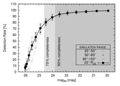
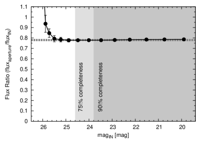
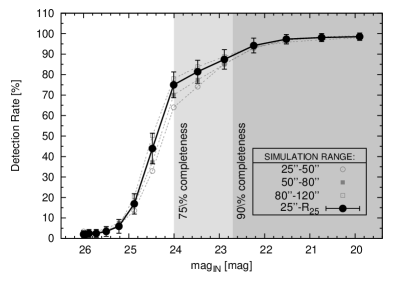
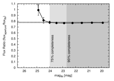
Figure 2: Results of the artificial source simulation for the $V$ (top) and $I$ (bottom) bands. The results were screened using the same criteria used to define the “GC candidates” sample ($\S$3.1). Left.- Detection rate (i.e. percentage of detected sources over simulated sources) as a function of the input magnitude. The shadowed areas delimit the 90% and 75% completeness regions. The bold line represents the detection rate for the simulation run between the detection limit ($R_{GC}=25~{}\arcsec$) and the galaxy $R_{25}$. The light gray lines represent the results from simulations run within limited galactocentric ranges. The dependence of the detection rate curves to the radial distance from the galaxy center has been properly taken into account when correcting the $V$ magnitude histogram for the effects of incompleteness (see $\S$4.1). Right.- Ratio of the aperture flux measured by SEXTRACTOR over the total input flux of the simulated source, as a function of the input magnitude. The median value for the data points over 75% completeness, represented by the dashed line, has been used to compute the aperture corrections applied to the fluxes of the real GCs (see $\S$2.2).

In order to evaluate the incompleteness of the GC samples (i.e., the fraction of GCs not detected due to faintness or issues related to the detection process), we set up an artificial source test to calibrate the SEXTRACTOR results. Simulated GCs were added to the NGC 4261 HST mosaics and their characteristics were measured with SEXTRACTOR using the same setup as for the real data. The simulation was repeated several times in order to improve the statistical results. The details of the artificial source test are described in Appendix A.

Figure 2 reports the simulation results for the $V$ (top) and $I$ (bottom) bands. The left panels of the figure show the detection rate (i.e. percentage of detected sources over simulated sources) as a function of the input magnitude. Input sources are detected with an efficiency of $\sim$90% (or higher) down to 23.8 mag and 22.7 mag for the $V$ and $I$ band respectively. We define these magnitudes as the detection thresholds. In order to assess the dependence of the completeness curves on the background light we repeated the simulation within 3 annulii located at different galactocentric radii (between the simulation limits $R_{GC}$ = 25$\arcsec$ and $R_{GC}$ = $R_{25}$). We found that the detection efficiency indeed shows a dependence on the brightness of the background, although the differences are significant only well below the 80% completeness level. The completeness correction applied to the $V$ band histogram in $\S$4.1 took this effect into account. Since the detection efficiency drops drastically for $R_{GC}<25~{}\arcsec$, we adopted this as the minimum galactocentric radius for the study of the spatial distribution of the sources ($\S$5). The right panels of Figure 2 show the ratio of the 0.5$\arcsec$ diameter aperture flux measured with SEXTRACTOR over the total input flux of the simulated sources, as a function of the input magnitude. At the faintest magnitudes, the flux ratio deviates from the constant value since the Poissonian variation of the background counts becomes an important contribution to the signal within the aperture. For this reason, we estimated the aperture correction only down to the 75% completeness limit. We find that our fixed 0.5$\arcsec$ aperture encompasses 79%, 78% and 77% of the flux for the $B$, $V$ and $I$ band respectively regardless of the size and shape parameters of the sources. These ratios are used as the aperture corrections for the magnitudes of the observed GCs (see $\S$2.2).

Figure 3 shows a histogram of the FWHMs of the real GCs (secure sample) compared with the FWHMs of the simulated objects (King profiles convolved with the instrument PSF). The excellent agreement between the two histograms, both at the “peak” and the “tail” of the distributions (the small discrepancies are most probably related to the fact that only one PSF model has been used for the whole mosaic), confirms that the simulated objects are representative of a population of GCs spanning the whole range of shape parameters (i.e., $r_{c}$ and $c$) expected for real sources. Moreover, it ensures that the “tail” of the FWHM distribution is not due to contamination by spurious sources, but it is produced by real GCs (and precisely by the most extended and faint). The “tail” contains a significant fraction of the sources; for example, the fraction of GCs with FWHM between 3 and 4 pixels equals 10% of the whole sample. In $\S$3.1, we reported that we imposed a FWHM limit of 4 pixels when selecting GCs. Based on the results of the simulation, we remark that choosing a more strict limit, although helping in excluding non-GC objects (e.g. galaxies), would also significantly reduce the number of real GCs in the candidate list.

We further tested the FWHM limits by simulating the most extreme faint and extended GCs and measuring their size. We defined the limiting magnitude for this simulation as that corresponding to the 90% completeness (calculated with the method described above, but excluding the FWHM criterion). We set the $c$ parameter to 2.0 and we chose a $r_{c}$ of 4 pc (0.26 pixels), which is in the upper range of observed core radii $r_{c}$ (see Jordán et al., 2005). The limiting FWHM found with this method was $\sim$4 pixels, in agreement with the adopted selection criteria.

Figure 3: Comparison of the FWHMs (in units of WFPC2 pixels) of the simulated sources (solid line) versus the FWHMs of the measured sources in the data (shaded histogram) for the $V$ band. The histograms are normalized to the total number of sources with FWHM between 0 and 4 pixels. This result is valid for the “GC candidates” sample (no colour selection was applied in this simulation).

4 Properties of the Globular Clusters

4.1 $V$ band Luminosity Function

The GC populations of almost all galaxies show a remarkable characteristic: their Luminosity Function (GCLF), plotted in magnitude units, is commonly represented by a Gaussian peaking at $M_{V}\sim-7.4$ mag, with a dispersion of $\sigma_{V}\sim 1.2$ mag (e.g. Harris, 1991; Ashman & Zepf, 1998), although minor deviations from this shape may be expected for a number of reasons (e.g. Jordán et al., 2007, Villegas 2010 for an extensive discussion on Gaussian representation of the GCLF in early type galaxies). A formation scenario that would justify a Gaussian distribution does not exist. Indeed, the GCLF has been tested against other types of distributions, e.g., the student $t_{5}$ function (Secker, 1992). For this reason, and given the skewness of the GCLF, the peak of the distribution is usually referred to as “turnover“. The location of the peak appears to be fixed and therefore, when expressed in terms of the apparent magnitude, it can be used to estimate the galaxy distance (Kundu & Whitmore, 2001).

The left panel of Figure 4 shows the $V$ band histogram for the candidate GCs (light gray), the secure sample of GCs (dashed shadow) and contaminating stars (gray shadow).

The expected contamination due to foreground stars has been evaluated using the TRILEGAL online tool (Girardi et al., 2005), which simulates the spatial distribution of stars in the Milky Way. Assuming models for the star formation rate, age-metallicity relation and initial mass function of the Galaxy, TRILEGAL computes the age, metallicity, mass and apparent photometry for the expected population of Galactic stars along the line of sight within the desired field of view. We queried the tool using the default parameters (Chabrier function for initial mass function, exponential disk model for extintion, thin disk + halo + bulge components for galaxy structure), for HST/WFPC2 (Vega system) magnitudes down to $m_{{}_{V}}$ = 28 mag and for a field equivalent to the size of the $D_{25}$ of NGC4261. Inspecting the histogram (Figure 4) we can see that the foreground star contamination is negligible. Moreover, this estimate should be considered as a rigorous upper limit, since this population was not filtered according to the selection procedure applied to the GCs ($\S$3.1).

4.1.1 Fitting The Luminosity Function Turnover

We fitted a Gaussian profile to the histogram of the secure (colour selected) GC sample (shown in Figure 4) in order to derive the peak location and FWHM of the GCLF.

Notice that the distributions appear as skewed Gaussians due to the cutoff imposed by the incompleteness at faint fluxes. In particular, due to the colour selection and the more significant effect of the incompleteness in the $I$ band data (caused by the higher background; see Figure 2), the faint end of the GCLF of the secure GC sample might be biased by the high $I$ band detection threshold. If this were to be the case, the result would appear as a deficit of blue objects at faint magnitudes. Instead, comparing the colour histograms of objects brighter and fainter than $m_{{}_{V}}>$24 mag, we find that such a selection effect is minimal.

Nevertheless, in order to obtain a conservative result, we estimated the magnitude at which such incompleteness starts affecting the sample using the following argument. The faintest object detected in the $I$ band, at the 75% completeness level, has a magnitude $m_{{}_{I}}\sim 24.0$ mag. Therefore, according to the minimum colour of the blue GC subpopulation ($V-I\sim$0.6 mag; see $\S$3.1), a faint blue GC is expected to have a $V$ magnitude of $\sim$24.6 mag (which is close to the 75% completeness level for the $V$ band). We adopted this value as the limit at which we “truncated” the fit of the GCLF.

The fit was performed using the Sherpa package v4.2.1 (which is part of the CIAO tool suite v4.2). The number of sources per bin of the Luminosity Function (LF) was high enough to allow the use of $\chi^{2}$ statistics. The uncertainties for each bin were estimated assuming a Poissonian distribution. The errors we report refer to the 1-$\sigma$ (68.3%) confidence bounds from the $\Delta\chi^{2}$ projection for 1 interesting parameter. The number of foreground stars and other contaminating objects has been accounted for by including a constant in the fit. The resulting value is compatible with the estimated number of contaminating stars per bin (see Figure 4).

The turnover of the GCLF is located at $m_{{}_{V}}$ = 25.1${}_{-0.6}^{+1.0}$ mag, and the Gaussian distribution has a FWHM of 3.1${}_{-0.8}^{+0.6}$ mag (or $\sigma$ = 1.3${}_{-0.3}^{+0.3}$ mag). Using the Third Reference Catalogue of Bright Galaxies (RC3; de Vaucouleurs et al. 1995) we verified that reddening effects on peak location are negligible ($\Delta_{B-V}$ = 0.02 mag). The large errors on the peak location and FWHM are a consequence of the necessity of truncating the fit around the turnover. Nevertheless, the best fit FWHM value is in close agreement with the results for the sample of elliptical galaxies studied by Kundu & Whitmore (2001) using data obtained with a similar configuration (WFPC2, filters F555W and F814W). The results of the fits are shown in Figure 4 and Table 2.

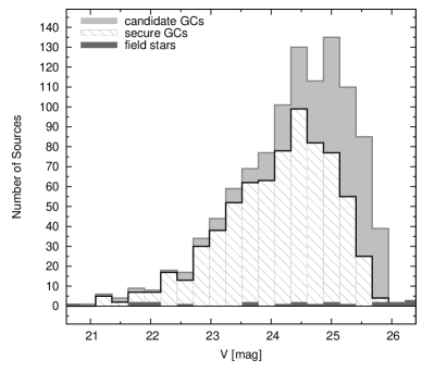
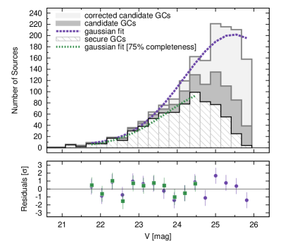
Figure 4: $V$ magnitude histograms for the GCs candidates and Gaussian fit. Left. ($V$ magnitude histograms) - Candidate GCs are shown in light gray, the subsample of candidate GCs selected in colour (secure GCs) with a dashed shadow and the contaminating stars (from the TRILEGAL simulation) in gray shadow. Right. (Incompleteness-corrected $V$ magnitude histogram and fits) - Candidate GCs are shown in light gray, the subsample of candidate GCs selected in colour (secure GCs) with a dashed shadow. The light gray area represents the distribution of the candidate GCs after applying the incompleteness correction, performed as described in $\S$3.2. The fit refers to the secure sample (green dashed line) and to the corrected candidate sample (violet dashed line). The bin sizes have been optimized according to the Freedman-Diaconis criterion (Freedman & Diaconis, 1981), using the mean photometric error as the minimum allowed value.

The turnover of the GCLF has been proven to be a reliable distance indicator (Kundu & Whitmore, 2001). Adopting a $M_{V}^{GC}=-7.4$ mag for the peak of the GCLF (with an error negligible in comparison to our photometric errors) we derived a distance modulus $m-M$ = 32.5${}_{-0.6}^{+1.0}$ mag. The corresponding distance is 31.6${}_{-8.7}^{+14.6}$ Mpc, in agreement with the estimate by Jensen et al. (2003) (29.4 $\pm$ 2.6 Mpc) based on surface brightness fluctuations. Tully & Fisher (1988) measured a heliocentric velocity $v$ = 2202 $\pm$ 75 km/s for NGC 4261, accounting for the infall of the Local Group to the Virgo cluster according to the model described in Tully & Shaya (1984). This velocity corresponds to a distance of 31.3 $\pm$ 1.2 Mpc (adopting an $H_{{}_{0}}=70.4\pm 1.4$ km/s/Mpc - Seven Years WMAP Observations; Jarosik et al., 2011), which is consistent with our measurement at the 1-$\sigma$ level.

Table 2: GCLF FIT RESULTS

Sample	Peak	FWHM	Amplitude†	Constant†	Integrated Number	Distance	$S_{N}$
	[mag]	[mag]			of Sources	[Mpc]
Secure GCs	25.1${}_{-0.6}^{+1.0}$	3.1${}_{-0.8}^{+0.6}$	101${}_{-21}^{+53}$	1.2${}_{-1.2}^{+4.6}$	1242	31.6${}_{-8.7}^{+14.6}$	1.5$\pm$0.3
Candidate GCs	25.5${}_{-0.2}^{+0.2}$	3.0${}_{-0.3}^{+0.4}$	196${}_{-12}^{+14}$	5.2${}_{-3.9}^{+3.2}$	2363	38.0${}_{-3.5}^{+3.5}$	2.8$\pm$0.5

$\dagger$ Value of [central] bin. Bin size: $\Delta$$V$ = 0.27 mag.

4.1.2 GC Specific Frequency

The GC Specific Frequency (SFs; number of GCs per unit luminosity) of a galaxy is defined as $S_{N}=N_{GC}\times 10^{0.4(M_{V}+15)}$ (Harris & van den Bergh, 1981).

An estimate of the total number of GCs ($N_{GC}$) within the $D_{25}$ was determined for both the secure and the candidate GCs by fitting their histograms with a Gaussian and a constant which accounted for contaminating objects. The LF for the candidate GCs sample had been previously corrected for incompleteness effects by splitting the sample into the three galactocentric ranges defined in Figure 2, applying the corresponding detection rate curve, and then stacking back the results into one histogram, shown in Figure 4. The parameters of the best fit Gaussian are shown in Table 2.

Notice that the distance modulus derived from the fit of the LF for the candidate GCs (see Table 2 and $\S$4.1.2) is evidently overestimated. The peak of the Gaussian is driven towards fainter fluxes where the contamination by spurious sources is amplified by the high completeness correction factor applied. Unfortunately, these sources cannot be distinguished from real GCs using the FWHM and elongation criteria. For this reason, the total number of GCs resulting from the candidate sample should be considered as un upper limit. On the other hand, the number derived from the secure sample, which was not corrected for incompleteness, represents a lower limit

The integral of the GCLF models yielded $N_{GC}\sim$1242 and $N_{GC}\sim$2363, for the secure and candidate sample respectively. Assuming an integrated magnitude for the galaxy of $m_{{}_{V}}$ = 10.01 $\pm$ 0.06 mag (derived as described below) and a distance of 29.4 $\pm$ 2.6 Mpc (Jensen et al., 2003), we calculated that: $S_{N}=$1.5 $\pm$ 0.3 for the secure sample and $S_{N}=$2.8 $\pm$ 0.5 for the candidate sample. Both numbers are within the range of typical values for elliptical galaxies (e.g. Kundu & Whitmore, 2001).

The galaxy asymptotic magnitude was determined from a $2D$ fit performed on the $V$ band WFPC2 data using GALFIT (Peng et al., 2002). This software is able to fit the surface brightness distribution of a galaxy to a $2D$ model accounting for the effect of $PSF$ blurring. We chose a Sersic model (plus a constant component accounting for the sky flux) and used the SEXTRACTOR results for the galaxy as initial fit parameters. We used a TinyTim $PSF$ image (generated as described in $\S$3.2), while we let GALFIT produce the weight image independently. We also applied a mask to exclude the central dust ring from the fit. The best-fit model has a Sersic index of 5.7, effective radius of $\sim$70$\arcsec$, major axis Position Angle (P.A.) of -21 deg and axis ratio ($b/a$) of 0.8. The ratio of the sum of residuals over the model-integrated light is less than 2% for all the filters, indicating that the model is a good representation of the starlight distribution of this galaxy. The galaxy magnitude was derived from the integral counts under the model applying the conversion formulae of Holtzman et al. (1995a).

The model-subtracted image showed a residual light ring around the galactocentric radius $R_{GC}\sim 15\arcsec$, while we did not find evidence for the tidal arm reported by Tal et al. (2009) (probably due to the lower exposure time). The peculiar pattern of the residuals is most likely related to the boxy nature of the galaxy. GALFIT is able to fit a boxy model with a fixed boxiness, while probably the isophotes of NGC 4261 have a radial variation in this parameter (such behavior has been reported in many ellipticals; e.g. Nieto & Bender, 1989).

4.2 Colour Distribution

An important result regarding GCs in massive galaxies is their bimodal colour distribution (e.g. Ashman & Zepf, 1998; Peng et al., 2006), generally attributed to a metallicity difference between two subpopulations (e.g. Brodie & Strader, 2006). There are different scenarios which can account for such bimodality. The best supported is probably the merging scenario, according to which the bluer (i.e., metal poorer) GCs are “donated” by merging galaxies, while the red (i.e. metal richer) GCs are formed in the merger, along with the bulk of the galaxy field stars (Ashman & Zepf, 1992). This model has the advantage of naturally explaining the subpopulations and their different radial distributions (see Section $\S$5), but does not address the extent to which the newly formed GCs can account for the significantly higher SF measured in elliptical galaxies with respect to those of the spiral galaxies (e.g. Harris, 1991), which are supposed to be their progenitors. It is also not yet clear whether a significant fraction of the young star clusters formed in merging galaxies can survive to account for the red GCs population of ellipticals. Valid alternatives are the multi-phase dissipational collapse model (Forbes, Brodie, & Grillmair, 1997), which assumes that blue and red GCs are formed at different stages of the galaxy formation, and the accretion scenario (Cote, Marzke, & West, 1998), in which the red GCs represent the intrinsic GC population of the galaxy while the blue GCs are acquired from lower mass galaxies during dry mergers or by tidal stripping. As reviewed by Brodie & Strader (2006), the three models are not mutually exclusive, and their effects may sum to generate the observed GC subpopulations in ellipticals.

Figure 5 shows the $V$-$I$ histogram for the secure GCs sample. The GC colour distribution doesn’t show the clear bimodality typical of the GC colour distribution in early-type galaxies (e.g. Brodie & Strader, 2006). In order to quantitatively discern the number of components in the distribution, we performed a mixture model analysis using the NMIX method of Richardson & Green (1997), which implements a Bayesian test of univariate normal mixtures. We run the code following the suggestions reported in Richardson & Green (1997) about the priors and hyperpriors (namely, choosing $\xi$ = 1.1, $K$ = 2, $h$ = 2, and setting the rest as default), even though the test was demonstrated to be robust with respect to the choice of the initial parameters. The test did not show significant evidence for a bimodal GC colour (Bayes factor of 1 and 0.5, for the unimodal and bimodal models respectively). However, the range of colours of our GC sample spans the typical colours of both the blue and red GCs in elliptical galaxies, while it is too wide to arise from a single GC population, suggesting that most probably the two subpopulations are blended in our data. Moreover, as pointed out by Peng et al. (2006) in their work on early-type galaxies in the Virgo cluster, even for those galaxies in which the relatively low number of GCs does not allow one to distinguish between unimodal and bimodal colour distributions, the result of a decomposition into two components provides a reliable description of the system. For these reasons, we assume that the distribution consists of superimposed blue and red subpopulations and so we fit the colour histogram using two Gaussian components, plus a constant to account for the contamination by foreground stars (estimated as 1-2 objects per bin using the TRILEGAL results - see $\S$4.1) and background galaxies. The uncertainties for each bin were estimated assuming a Poissonian distribution.

Table 3 reports the result of the fit. For completeness, the table also shows the result from a single Gaussian fit. In the double-component case, the large errors in the Gaussian normalizations reflect the fact that the two amplitudes are strongly correlated. Nevertheless, the locations of the peaks are accurate enough to allow us to identify a blue and a red subpopulation, with average colours $V$-$I$=1.01${}_{-0.06}^{+0.06}$ mag and $V$-$I$=1.27${}_{-0.08}^{+0.06}$ mag respectively. These values are in good agreement (within 1$\sigma$) with those reported by Larsen et al. (2001) based on a similar analysis of the GC population of a sample of nearby early-type galaxies, observed using deep exposures in the F555W ($V$) and F814W ($I$) HST filters.

The best-fit model along with the individual components are shown in the top panel of Figure 5. The bottom panel shows the residuals with respect to the best-fit model in units of standard deviation.

Table 3: $V$-$I$ FIT RESULTS

DOUBLE COMPONENT
Component	Amplitude†	Peak	FWHM
		[mag]	[mag]
Blue Gaussian	59${}_{-29}^{+23}$	1.01${}_{-0.06}^{+0.06}$	0.30${}_{-0.06}^{+0.08}$
Red Gaussian	56${}_{-22}^{+15}$	1.27${}_{-0.08}^{+0.06}$	0.30${}_{-0.07}^{+0.1}$
Constant	6${}_{-3}^{+2}$	-	-
$\chi_{\nu}^{2}$ = 1.11, 10 d.o.f. ($P_{(Q-value)}$ = 35%)
SINGLE COMPONENT
Component	Amplitude†	Peak	FWHM
		[mag]	[mag]
Gaussian	81${}_{-4}^{+4}$	1.14${}_{-0.01}^{+0.01}$	0.49${}_{-0.04}^{+0.02}$
$\chi_{\nu}^{2}$ = 1.06, 14 d.o.f. ($P_{(Q-value)}$ = 39%)

$\dagger$ Value of [central] bin. Bin size: $\Delta$$V-I$ = 0.06 mag.

We arbitrarly divided the secure GCs into blue and red by setting the threshold at $V$-$I=$ 1.15. The discriminating value is representative of the 50% probability for a GC to belong to the blue or red subpopulation (the intersection of the Gaussians in Figure 5). This value is consistent with the separation of the two subpopulations in other galaxies (e.g. Ashman & Zepf, 1998).

In order to estimate the relative abundance of the blue and red subpopulations, we performed the following Monte-Carlo simulation. We sampled each of the parameters of the two-Gaussian fit (described above). The sampling distribution was a multi-variate Gaussian with a mean equal to the best-fit value of each parameter and a FWHM derived from the covariance matrix of the fit. At each trial, the set of sampled parameters defined two Gaussians whose flux fractions with respect to the total flux from the combined model were recorded. Finally, the expectation value for the fraction of the blue/red component was calculated as the median over all the trials. With this method, we estimated that the blue (red) GCs represent the 60${}_{-24}^{+21}$% (40${}_{-21}^{+24}$%) of the total sample of 718 GCs. The upper and lower uncertainties on the fraction represent the 68.3% quantile (1 $\sigma$) around the medians.

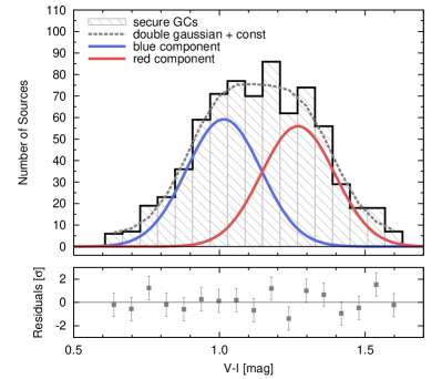
Figure 5: $V$-$I$ colour histogram for the secure GCs sample and fit. The data have been fit using two Gaussians plus a small constant used to account for contamination. In the figure, we show the two Gaussian components (blue and red dotted lines) and the total convolved model (gray dashed line). The additive constant is not showed in the figure. The bin sizes have been optimized according to the Freedman-Diaconis criterion (Freedman & Diaconis, 1981), using the mean photometric error as the minimum allowed value.

5 Spatial Distribution of Sources

Prompted by the findings of Zezas et al. (2003) and Giordano et al. (2005), we investigated the spatial distribution of the secure GC sample.

The region of the galaxy within $R_{GC}<$ 25″ was excluded from the analysis due to the high background which drastically limited the source detection sensitivity (see $\S$3.2). Since the GC detection rate depends on the galactocentric distance (Figure 2) and affects the relative number of detected sources at each radius, introducing artificial asymmetries, we decided to limit the analysis to those GCs having a magnitude brighter than the 75% completeness limit for the $V$ band (corresponding to $m_{V}$ = 24.6 mag).

5.1 Radial Distribution

In the top panel of Figure 6 we present the radial profiles of the blue and red GCs. As a reference, we also plot a scaled $V$-band light profile model of NGC 4261 (as derived from the GALFIT fit; see $\S$4.1.2). The data points represent the surface densities (number of sources per arcsec²) over elliptical annulii centered on the galaxy center. The orientation and ellipticity of the annulii have been chosen to match the P.A. and ellipticity of the galaxy light profile. The profiles have been normalized to match at the first point.

We used funtools (Mandel, Murray, & Roll, 2001) to count the number of sources within each annulus. The annulii sizes (i.e. binning of the plot) have been chosen in order to contain a statistically significant number of sources (at least 20 sources per bin) that would allow the use of a $\chi^{2}$ test. The uncertainty for each bin is simply the square root of the counts divided by the annulus area.

The distribution of the overall GC population looks consistent with the trend of the light profile, at least from the galaxy center up to $R/R_{25}$ = 0.75, where it starts declining, mostly driven by the drop of the red GC component. The difference between the trends of the blue and the red GCs radial profiles is more evident when the distributions are plotted in terms of Specific Frequency ($S_{N}$), calculated as $S_{N}(i)=N_{GC}^{i}\times 10^{0.4(M_{V}^{i}+15)}$ , where $i$ is the annulus index (bottom panel of Figure 6). In fact, recalling that $S_{N}$ expresses the relation between the number of clusters and the galaxy light, the systematic decrease of $S_{N}^{{}_{RED}}$ denotes a clear inconsistency with the galaxy surface brightness. On the other hand, $S_{N}^{{}_{BLUE}}$ varies around a constant value.

Such behaviour seems to be in contrast with the commonly accepted scenario (see $\S$4.2) according to which the red (young) GCs follow the galaxy light, while the blue (old) are spread almost uniformly (e.g. Brodie & Strader 2006; Ashman & Zepf 1998).

On the other hand, the strong blending of the colours of the two populations of our sample (see $\S$4.2) may not have allowed us to separate properly the two profiles.

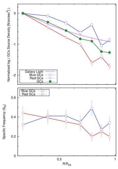
Figure 6: GCs radial profiles. Top. Comparison of the source densities of the GCs sample (defined in Section $\S$5) and of the blue and red subpopulations (green, blue and red lines respectively) with the scaled light profile model of the galaxy (violet line). The data points represent the source densities evaluated over elliptical annulii. The radial coordinate is expressed in terms of the galaxy semi-major axis $R_{25}$ = 2.04″. The vertical error bars represent Poissonian errors. The profiles have been normalized in order to match at the radius of the first annulus. Bottom. Radial profile of the Specific Frequency ($S_{N}$) of the blue and red subpopulations (blue and red lines respectively), calculated as $S_{N}(i)=N_{GC}^{i}\times 10^{0.04(M_{V}^{i}+15)}$, where $i$ is the annulus index.

A Kolmogorov-Smirnov (K-S) test has been used to compare the radial distribution of blue and red GCs against a Sersic brightness profile (whose parameters have been derived from the GALFIT fit; see $\S$4.1.2). Since the Sersic profile is defined assuming circular symmetry, the dependence of the galactocentric distance of a GC ($R_{GC}$) on the ellipticity of the galaxy had to be removed as well. The variable used to perform the test was the major axis $a$ of the ellipse intercepting the GC and defined by the same center, elongation and P.A. as for the galaxy. This can be calculated as:

$$a_{i}={{R_{GC,i}\times\sqrt{e^{2}\cos^{2}(\theta_{i}-P.A.)+\sin^{2}(\theta_{i}-P.A.)}}\over{e}}$$ (5)

where $e$ is the elongation, $\theta$ the azimuthal angle ($\theta$ = 0 towards North and increases counterclockwise) and $i$ the GC index. The test returned a probability well below the 0.1% level for the blue GCs and a probability of 0.3% for the red GCs, therefore rejecting the null hypothesis that their radial distributions follow the galaxy light profile.

5.2 Azimuthal Distribution

We evaluated the azimuthal distribution of the overall GC sample as well as of the blue and red subpopulations by comparing their source densities against the galaxy surface brightness within a set of elliptical wedges centered on the galaxy nucleus. The parameters of the ellipses (center, ellipticity) have been obtained from the GALFIT fit (see $\S$4.1.2). The angular extent of the wedges has been chosen to ensure Gaussian statistics for the majority of the bins ($>$20 sources per bin).

In our mosaics, 4 areas within the galaxy $D_{25}$ were covered by the WFPC2 PC camera (field of view of 35$\arcsec$$\times$35$\arcsec$). We had to exclude these locations from the current analysis due to their different sensitivity (which would influence the surface brightness estimation) and higher noise (which could create artificial deficits of GCs). When measuring the galaxy light, we also masked out all the GCs (secure sample), foreground stars and background galaxies.

The measurements were repeated for different rotations (offsets) of the ellipse wedges in order to address the significance of any density excess. The wedge offset is defined on the rotation of a complete set of wedges measured counterclockwise with respect to the North. For each offset, a $\chi^{2}$ test between the azimuthal profiles of the GC density and that of the galaxy light has been performed in order to identify the wedge rotation for which the anisotropy is maximized. Notice that, in this context, the azimuthal surface brightness distribution of the galaxy simply represents a uniform comparison distribution which also includes the modulation due to the geometry of the wedges alone.

Figure 7 shows the source density azimuthal profile of the whole GC sample as well as the blue and red subpopulations for the wedge-offset that maximizes the $\chi^{2}$ statistic for each series. The solid lines represents the best-fit of the galaxy light to each data series (used to calculate the $\chi^{2}$). The counter-intuitive modulation of the azimuthal distribution of the galaxy light is due to a combination of two effects: the boxiness of the galaxy (so that the wedges along the major axis have larger areas but include less flux), and the masking we applied. The bottom panel of the figure reports the fit residuals expressed in terms of $\sigma$ with respect to the fitted model (i.e. starlight distribution).

The plot shows a clear density enhancement (more than 2 $\sigma$) at P.A. $\sim$225$\pm$18^∘, and significant deficits at P.A. $\sim$120$\pm$18^∘ and at P.A. $\sim$270$\pm$18^∘. The peak-to-peak variation is of the order of several $\sigma$; the red GC subpopulation seems to follow the same modulation, while the statistics for the blue distribution are too poor to derive any conclusion.

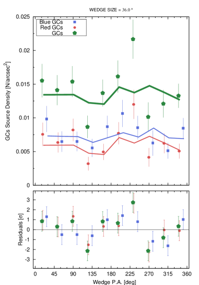
Figure 7: Source density azimuthal profile. The data points represent the density of GCs within wedges of 36^∘ for the GCs sample (green diamonds) and for the red and blue subpopulation (red dots and blue squares respectively) as a function of the wedge P.A., for the wedges offset maximizing the anisotropy of each series (P.A. = 0 towards North and increases counterclockwise). The solid lines represent the best fit of the galaxy light to each data series. The bottom panel of the figure reports the scatter of the three data series with respect to the fit in units of $\sigma$. The data points have been slightly shifted along the $x-axis$ for presentation purposes.

The GCs in the overdensity regions do not show any difference in brightness or colour distribution with respect to the “field” GCs (the KS test can not distinguish the two distributions), their $V$ and $V-I$ histograms closely resembling the ones of the whole secure GCs sample (shown in Figures 5 and 4).

This test showed that the reduced $\chi^{2}$ ($\chi_{\nu}^{2}$) for the whole sample was as high as 2.5 for 9 degrees of freedom. Since we deliberately select the highest $\chi_{\nu}^{2}$, the usual $\chi_{\nu}^{2}$ probability density function will not provide a correct confidence level. Instead, we had to compare this value against the $\chi_{\nu}^{2}$ generated by a population of GCs distributed according to the galaxy light, in order to exclude the possibility that the overdensities of GCs are statistical fluctuations. To reproduce the proper $\chi_{\nu}^{2}$ probability distribution, we performed the following test. We generated $n$ points (where $n$ equals the number of wedges) distributed according to a Poissonian density function around the average number of GCs found within a wedge. Such a set of data represented the equivalent of the GCs azimuthal profile measured for a certain wedge rotation. The data were then fit with a constant. The correct way to run this test would have been to use the galaxy light azimuthal distribution to derive the average of the Poissonian distribution in each wedge, but, since we assume a constant $N_{GC}$ to light ratio in each wedge, the two methods are exactly equivalent (in the latter case the appropriate fit would just be a rigid shift of that curve along the y-axis). We simulated a set for each wedge offset and we recorded the maximum $\chi_{\nu}^{2}$ among the sets, as for the real data.

The whole simulation was repeated 2000 times in order to generate the $\chi_{\nu}^{2}$ probability distribution. The histogram in Figure 8 shows the resulting distribution of the simulated max $\chi_{\nu}^{2}$. The arrow shows the value of the $\chi_{\nu}^{2}$ measured from the data. The integral of the simulated $\chi_{\nu}^{2}$ exceeding this value corresponds to a probability $P_{\chi_{\nu}^{2}>\chi_{\nu,obs}^{2}}$ $<$ 0.1%. This result indicates that the asymmetry in the azimuthal distribution of the GCs with respect to the galaxy light is statistically significant at the 99.9% level.

Figure 8: Probability distribution of $\chi_{\nu}^{2}$ produced by the fit of a constant to random sets of 10 data points distributed according to a Poisson distribution. The simulation is meant to reproduce the $\chi_{\nu}^{2}$ derived for a uniform azimuthal distribution (see text for more details). The arrow represents the $\chi_{\nu}^{2}$ obtained fitting the azimuthal distribution of the GCs to the galaxy light. The area covered by $\chi_{\nu}^{2}$ equal or higher than this value corresponds to a probability $P_{\chi_{\nu}^{2}>\chi_{\nu,obs}^{2}}$ $<$ 0.1%, therefore indicating that the asymmetry in the azimuthal distribution of the GCs with respect to the galaxy light is statistically significant.

As a further test, we compared the distributions of the candidate GCs, and the blue and red subpopulations, against a uniform distribution using a K-S test. The KS test results did not allow us to reject the null hypothesis (i.e., that the azimuthal profile follows a uniform distribution), for either of the three GCs subpopulations (we obtained probabilities of 7%, 35% and 73% for the whole sample and the blue and red subpopulations, respectively). In order to assess the significance of this result, we calibrated the K-S test in a similar fashion as for the $\chi^{2}$ method. For each population (secure GCs, red subpopulation and blue subpopulation), we generated $m$ random angles (where $m$ is the number of sources in the population) uniformly distributed in the range $[0,2\pi]$. The cumulative distribution of this sample was compared against the cumulative of a uniform distribution and the maximum distance $D$ between the two was recorded (such distance is in fact the K-S statistic). The simulation was repeated 10000 times in order to generate the probability distribution for $D$. The integral of the values exceeding the $D$ measured in the K-S test on the real data correspond to the probabilities $P_{D>D_{obs}}^{GCs}\sim 10\%$, $P_{D>D_{obs}}^{red}\sim 70\%$ and $P_{D>D_{obs}}^{blue}\sim 30\%$ for the secure GCs sample and the red and blue subpopulations, respectively. This result confirmed that the K-S test is not sensitive enough to identify the differences seen between the samples.

5.3 The two-Dimensional Distribution of the GC Population

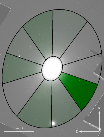
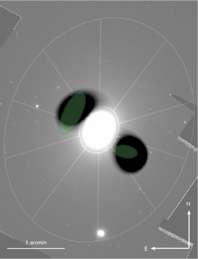
Figure 9: Local enhancements of GCs. Left. Over a mosaic of NGC 4261 ($I$ band), we overlay the sectors over which we evaluated the GC azimuthal densities shown in Figure 7 (black ellipse). The inner and outer radius of the ellipse correspond to $R_{GC}$ = 25$\arcsec$ and $R_{GC}$ = $R_{25}$ respectively. The elliptical annular wedges we show are rotated to the angles at which the anisotropies in the GC azimuthal distribution are maximized. The filled wedges map the density enhancements shown in Figure 7: the color intensity is proportional to the significance of the excess (i.e. value of the corresponding - positive - residual in bottom panel of Figure 7). Right. Overlaid on a mosaic of NGC 4261 ($I$ band), the shaded ellipses show local enhancements in the distribution of GCs detected with a Voronoi Tesselation and Percolation (VTP) algorithm. Each clustering is represented by an ellipse whose axes size equals the $\sigma$ of the spatial distribution of its GCs. The black shadows represent the areas of higher clustering of the secure GC sample as detected by the CIAO task csmooth. The results from the VTP algorithm and from csmooth are clearly consistent with those from the wedges test, and they point to a GC density excess along a NE-SW direction.

In order to further investigate any local enhancements in the spatial distribution of the GCs we used the CIAO tools csmooth and vtpdetect.

These tools were originally designed to identify clusters of photons in X-ray images. For this reason, we created “images” of the GC locations to be used by the tasks, with pixel value equal to 1 where a GC was present and 0 elsewhere.

The csmooth tool smooths the image using an adaptive Gaussian kernel: the scale for each area is increased until the counts under the smoothing kernel exceed the significance threshold over the (local) background set by the user. We set a minimal significance threshold of 3 $\sigma$. The background, which in our case represents the uniform component of the GCs distribution, has been estimated locally. The task is robust with respect to the modification of the other parameters (such as the initial guess of the smoothing scale), which mostly affected the computational time.

The result of this procedure is shown in Figure 9. We can clearly identify two regions where the clustering of GCs appears to be significant (the regions appear slightly curved since we excluded sources near the center of the galaxy). These enhancements in the source density are located around P.A.$\sim$30^∘ and P.A.$\sim$245^∘ (NE and SW regions), in agreement with the locations of the peak in the azimuthal distribution of GCs (Figure 7).

The vtpdetect task exploits the Voronoi Tessellation and Percolation (VTP) technique to detect connected sets of photons above a threshold density. In our case, each GC played the role of a distinct photon. The task “cuts out” a triangular area around each source and calculates the source density (number/area). The background model is estimated by fitting the low-end of the cumulative density function (CDF). A density cutoff (used to distinguish areas containing a source photon from background) is derived from the residual between the CDF and the background model. Contiguous areas over the density cutoff are then clustered together using a percolation algorithm. A source built in this way is considered significant if it exceeds the desired false source limit due to background fluctuations. A detailed description of the VTP theory is presented in the CIAO Detect Reference Manual (December 2006).

In order to use vtpdetect on non X-ray data we had to deduce the task parameters through a trial-and-error approach. We estimated a GC “flux cutoff” comparing the source density in the outer regions of the image against the average area per source. The result was compatible with the default value for the relevant task parameter (maxbkgflux = 0.8). We adopted the default values also for the other parameters related to the background estimation (mintotflux = 0.8, maxtotflux = 2.6, mincutoff = 1.2, maxcutoff = 3), after verifying that they did not significantly affect the detection results. We set limit = 0.001 and scale = 1; these values have been chosen in order to limit the source deblending.

The 1$\sigma$ VTP ellipses defining source clustering are shown in Figure 9. The results from the VTP test confirm the excess detected by csmooth.

6 Discussion

Using $HST$ WFPC2 data in the $B$, $V$ and $I$ band (HST filters F450W, F606W and F814W, respectively) we characterized the GC population of the nearby elliptical galaxy NGC 4261. We studied the Globular Cluster Luminosity Function (GCLF), deriving a total number of $\sim$2363 GCs, corresponding to a Specific Frequency (SF; number of GCs per unit magnitude) of 2.8$\pm$0.5. From the location of the peak of the GCLF, we derived a distance of 31.6${}_{-8.7}^{+14.6}$ Mpc (assuming a $M_{V}\sim-7.4$ mag - e.g. Harris 1991; Ashman & Zepf 1998). The colour distribution can be interpreted as the superposition of a red and a blue subpopulation, with average colour $V-I$ = 1.01${}_{-0.06}^{+0.06}$ mag and 1.27${}_{-0.08}^{+0.06}$ mag respectively.

Most importantly, we used different techniques to study the two-dimensional distribution of the GCs sample and its blue and red subpopulations. As discussed in $\S$5.2 and $\S$5.3, we discovered that the GC population of NGC 4261 shows evidence for an asymmetry in the azimuthal distribution above the 99.9% confidence level. A similar effect is noticed in the red GC subpopulation, but on at lower significance. The result for the blue GCs is not statistically significant. The origin for such anisotropy may reside in the evolution of the galaxy in the recent past. Next, we discuss possible scenarios that address to this asymmetry.

1. Major merging event. The effects of a major merging event represent the most obvious candidate to explain such a significant asymmetry. NGC 4261 does not show signs of recent strong interactions (shells, ripples, arcs, tidal tails or other distortions), therefore we exclude a major merger within the last 1 Gyr, since this is the timescale on which interaction features fade away (e.g. Quinn, 1984; Hernquist & Quinn, 1988, 1989). The difference between the starlight and GC distributions implies that, if the GC asymmetry is related to a major merger event (whether new GCs have been formed in situ, donated or just been displaced), the relaxation timescale for the GC population is larger than for stars. This is a complicated issue since GC systems extend beyond the main stellar body of the galaxy, and their dynamics at large galactocentric radii are affected by the dark matter (resulting in higher velocity dispersions for the GCs than for the stars). To our knowledge, there is no reported evidence for such a difference in the relaxation time so far.

   A major merging event may have triggered episodes of star formation within remnant tails along the line of sight. In this case, the enhanced GC density along the NE-SW axis of NGC 4261 may just be due to a projection effect. Studies of galaxies at an advanced state of merging, such as NGC 7252, NGC 3256 or NGC 3921 (Knierman et al. 2003; Schweizer et al. 1996) show indeed that tidal tails host significant populations of proto-GCs. Therefore a certain fraction of GCs form in highly asymmetric distributions. The question is what fraction of these proto-GCs can survive tidal destruction and whether they can maintain their original spatial asymmetry during the subsequent dynamical evolution of the host galaxy.

   In addition, there are cases suggesting incomplete violent relaxation which would naturally result in non uniform distribution. Schweizer et al. (1996) showed that the candidate GCs of the protoelliptical NGC 3921 may have experienced the same (incomplete) violent relaxation as did the average starlight. Nevertheless, their data (although only partially covering the galaxy extent) show indications of asymmetry both in the radial and in the azimuthal distribution of the GCs. This suggests that spatial asymmetries of GC systems may indeed survive the relaxation process.

   Numerical simulations suggest that massive boxy ellipticals (such as NGC 4261) are most probably the result of dissipationless (dry) mergers between ellipticals of similar size (e.g. Khochfar & Burkert, 2005; Naab, Khochfar, & Burkert, 2006). Since this scenario does not involve gas, or all the gas is converted to stars prior to the collapse, the number of newly formed GCs along tidal tails would be negligible.

   Moreover, according to the merging scenario, the displaced GCs should mostly be younger (i.e. metal-rich). Since we observe asymmetry in both the blue and red subpopulations (although the result for the blue GCs is not statistically significant), we may conclude that the former hypothesis does not apply in the case of NGC 4261.

   Given the forementioned considerations, we conclude that a major merging event may be responsible for the observed asymmetry only if the relaxation timescale for the GC population could be proven to be larger than for stars.

2. Minor merging event. As mentioned above, the absence of fine structure in NGC 4261 excludes the possibility of a recent ($\sim 1$ Gyr) major merging, but it does not rule out this possibility for minor mergers, since these events have weaker effects on the galaxy light distribution. This is the case in the elliptical galaxy NGC 1052, which underwent a recent (1 Gyr) merging event with a gas rich dwarf (van Gorkom et al., 1986). The galaxy shows a weak rotation about its minor-axis (suggesting triaxiality) and significant minor-axis position angle swings (see notes in Davies & Birkinshaw, 1988), but, similarly to NGC 4261, it exhibits a very low fine structure parameter (Schweizer & Seitzer, 1992). Pierce et al. (2005) though, found no young GCs associated with the recent merger event of NGC 1052. This may indicate that no significant increase in the GC population should be expected even in case of gas rich minor merging.

   Non-relaxed GC distributions can be easily explained by GCs donated in a recent minor merging event but their number densities would be too small to generate statistically significant asymmetries over the galaxy light background. On the contrary, we can not rule out the possibility that the “indigenous” GCs have just been displaced during the merger.

3. Galaxy interactions. Galaxy interactions are known to provoke displacements of the GCs systems. For example, the flyby encounter of NGC 1399 with the nearby NGC 1404 disturbed the velocity structure of the outer regions of the GC system of NGC 1399 (Napolitano, Arnaboldi, & Capaccioli, 2002), or even generated a “tidal stream” of intergalactic GCs (Bekki et al., 2003). A smoothed map of the displaced blue GCs candidates around NGC 1399 is reported in Bassino et al. (2006, Figure 9).

   Moreover, simulations by Vesperini & Weinberg (2000) showed that the perturbations on stellar systems of elliptical galaxies due to flyby encounters can last well past the closest passage of the perturber. Similarly, we can expect that the asymmetric distribution of the GC system of NGC 4261 may be a remnant from the recent interaction with one of its close by companions. In order to identify the candidate perturber, we calculated the RMS radial velocity of the members of the NGC4261 group (Garcia, 1993) and, considering a time between 1 and 2 Gyr for the remnants of the interaction to disappear, we estimated that the perturber should be found between 15$\arcmin$ and 30$\arcmin$ off NGC 4261. Unfortunately, even considering only the brightest galaxies ($g$ $<$ 14 mag) in this range, there are too many candidates to uniquely identify the possible perturber.

   In this sense, a close encounter similar to the one that happened between NGC 1399 and NGC 1404 may have shifted some of the GCs of NGC 4261 from the NW-SE “poles” towards the NW-SE edge-on plane, with the galaxy nucleus preventing us from observing the distribution at the innermost radii. The GC systems extend much further than the host galaxy light, therefore the displacement may have affected only the outermost GCs without affecting the stellar orbits and hence the starlight. This event may also justify the peculiar drop of the GC radial profiles at large radii, shown in Figure 6 (although the effect may be due only to statistical fluctuations). If the GCs are indeed distributed continuously along a NW-SE axis, they would lie along a plane perpendicular to the rotation axis (Davies & Birkinshaw, 1986), therefore the overdensity could be simply associated with the rotation of the galaxy.

   In addition, some GCs may have been stripped out of the interacting galaxy. However, since the candidate perturbers are significantly smaller than NGC 4261 (therefore they have poorer GC systems), this effect can not explain alone the azimuthal variation of the GC density. In fact, its variation can reach up to $\sim$ 50% (distance of the GC density from the fit of the galaxy surface brightness; Figure 7), requiring a number of stripped GCs comparable to the system of NGC 4261. We find that there is no evidence for a difference between the properties (colour, FWHM, axis ratio, etc.) of the objects in the overdensity regions and those in the “field”. This implies that the number of GCs subtracted from the interacting galaxy is relatively small or if the acquired GC population is numerically significant, then it has similar properties.

The displacement of GCs under the effects of galaxy interaction or mergers and estimation of the relaxation times for GC “particles” embedded in mixed baryonic and dark matter environments is a subject that needs to be explored in order to understand the distribution of the GC populations in the increasing number of galaxies which show non-uniform GC systems.

7 Conclusions

We performed an analysis of the characteristics and spatial distribution of the GC population of the nearby elliptical galaxy NGC 4261 using deep $HST$ WFPC2 data in the $B$, $V$ and $I$ band (HST filters F450W, F606W and F814W, respectively). Our photometry of the GC system resulted in a sample of 718 secure GCs, complete down to $m_{{}_{V}}$ = 23.8 mag (90% completeness level). We were able to derive the Globular Cluster Luminosity Function (GCLF) down to the limiting magnitude $V$ = 24.6 mag. The distribution peaks at $m_{{}_{V}}$ = 25.1${}_{-0.6}^{+1.0}$ mag, consistent with a distance of 31.6${}_{-8.7}^{+14.6}$ Mpc (assuming a peak $M_{V}\sim-7.4$ mag - e.g. Harris 1991; Ashman & Zepf 1998). We studied the colour distribution and probed the bimodal behaviour expected in elliptical galaxies for GC systems (e.g. Ashman & Zepf, 1998). The $V-I$ colour distribution is compatible with the superposition of a blue and a red component with average colour 1.01${}_{-0.06}^{+0.06}$ mag and 1.27${}_{-0.08}^{+0.06}$ mag respectively. We calculated a Specific Frequency (number of GCs per unit magnitude) of 2.8$\pm$0.5, therefore relating the GC abundance to the stellar mass. We analyzed the two-dimensional distribution of the GC sample, and we found that it shows evidence for an asymmetry in the azimuthal distribution above the 99.9% confidence level. A similar effect is noticed in the red GC subpopulation alone, but at a lower level of statistical significance. We discussed the origin of this anisotropy in context of galaxy interaction and evolution. Our main results regarding the GC spatial distribution are the following:

1. The GC radial profile follows the galaxy surface brightness especially at galactocentric radii $R/R_{25}<$ 0.6. The red subpopulation profile is systematically steeper than the starlight, while the profile of the blue subpopulation looks more consistent with it (Figure 6).

2. The azimuthal distribution of the GC population shows significant enhancements along a NE-SW direction (Figure 7 and 9). The red subpopulation seems to follow the same modulation, reflecting each local enhancement/deficit. The result for the blue GCs is statistically not significant.

3. We suggest that the peculiar asymmetric distribution may be related to a past (dry) merger or interaction event. In particular, we favour the hypothesis that a fly-by encounter displaced the outermost GCs. The hypothesis of a past (older than 1 Gyr) major merging event cannot be ruled out, modulo the assumption that the GC relaxation time is longer than for the stars. We remark that the GCs may be distributed on an edge-on plane, since the galaxy nucleus prevents us from observing the distribution at the innermost radii. If this were to be the case, we cannot exclude that the overdensities could be rotation-related.

The study of the anisotropy of the GC population of a galaxy is a relatively unexplored field, which offers the unique opportunity of exploiting the GCs to investigate the history of the host galaxy. Spectroscopic data are critical to investigate whether the GCs of NGC 4261 show any peculiar kinematics or they have typical dispersion velocities for elliptical galaxies. In particular, spectroscopy of the GCs in the overdensity regions will clarify whether they are displaced GCs and move as an independent system from the overall GC population. Finally, we enphatize the need for numerical simulations aimed at modelling the evolution of the GC spatial distribution after a galaxy interaction or a merger and at estimating the relaxation times for GC “particles”.

References

- Adelman-McCarthy et al. (2007) Adelman-McCarthy J. K., et al., 2007, ApJS, 172, 634
- Ashman & Zepf (1992) Ashman K. M., Zepf S. E., 1992, ApJ, 384, 50
- Ashman & Zepf (1998) Ashman K. M., Zepf S. E., 1998, gcs..book,
- Barmby, Holland, & Huchra (2002) Barmby P., Holland S., Huchra J. P., 2002, AJ, 123, 1937
- Barnes (1988) Barnes J. E., 1988, ApJ, 331, 699
- Bassino et al. (2006) Bassino L. P., Faifer F. R., Forte J. C., Dirsch B., Richtler T., Geisler D., Schuberth Y., 2006, A&A, 451, 789
- Bekki et al. (2003) Bekki K., Forbes D. A., Beasley M. A., Couch W. J., 2003, MNRAS, 344, 1334
- Bertin & Arnouts (1996) Bertin E., Arnouts S., 1996, A&AS, 117, 393
- Birkinshaw & Davies (1985) Birkinshaw M., Davies R. L., 1985, ApJ, 291, 32
- Bournaud et al. (2004) Bournaud F., Duc P.-A., Amram P., Combes F., Gach J.-L., 2004, A&A, 425, 813
- Brodie & Strader (2006) Brodie J. P., Strader J., 2006, ARA&A, 44, 193
- Clark (1975) Clark G. W., 1975, ApJ, 199, L143
- Cote, Marzke, & West (1998) Cote P., Marzke R. O., West M. J., 1998, ApJ, 501, 554
- Davis et al. (1995) Davis D. S., Mushotzky R. F., Mulchaey J. S., Worrall D. M., Birkinshaw M., Burstein D., 1995, ApJ, 444, 582
- Davies & Birkinshaw (1986) Davies R. L., Birkinshaw M., 1986, ApJ, 303, L45
- Davies & Birkinshaw (1988) Davies R. L., Birkinshaw M., 1988, ApJS, 68, 409
- de Vaucouleurs et al. (1991) de Vaucouleurs G., de Vaucouleurs A., Corwin H. G., Jr., Buta R. J., Paturel G., Fouque P., 1991, trcb.book,
- de Vaucouleurs et al. (1995) de Vaucouleurs G., de Vaucouleurs A., Corwin H. G., Buta R. J., Paturel G., Fouque P., 1995, yCat, 7155, 0
- Fabbiano (2006) Fabbiano G., 2006, ARA&A, 44, 323
- Fabian, Pringle, & Rees (1975) Fabian A. C., Pringle J. E., Rees M. J., 1975, MNRAS, 172, 15P
- Ferrarese, Ford, & Jaffe (1996) Ferrarese L., Ford H. C., Jaffe W., 1996, ApJ, 470, 444
- Forbes, Brodie, & Grillmair (1997) Forbes D. A., Brodie J. P., Grillmair C. J., 1997, AJ, 113, 1652
- Forbes et al. (2004) Forbes D. A., et al., 2004, MNRAS, 355, 608
- Freedman & Diaconis (1981) Freedman D., Diaconis, P. 1981 Probability Theory and Related Fields Heidelberg: Springer Berlin, 57, 453
- Garcia (1993) Garcia A. M., 1993, A&AS, 100, 47
- Gehrels (1986) Gehrels N., 1986, ApJ, 303, 336
- Giordano et al. (2005) Giordano L., Cortese L., Trinchieri G., Wolter A., Colpi M., Gavazzi G., Mayer L., 2005, ApJ, 634, 272
- Girardi et al. (2005) Girardi L., Groenewegen M. A. T., Hatziminaoglou E., da Costa L., 2005, A&A, 436, 895
- Harris & van den Bergh (1981) Harris W. E., van den Bergh S., 1981, AJ, 86, 1627
- Harris (1991) Harris W. E., 1991, ARA&A, 29, 543
- Harris (1996) Harris W. E., 1996, AJ, 112, 1487
- Hernquist & Quinn (1988) Hernquist L., Quinn P. J., 1988, ApJ, 331, 682
- Hernquist & Quinn (1989) Hernquist L., Quinn P. J., 1989, ApJ, 342, 1
- Holtzman et al. (1995a) Holtzman J. A., Burrows C. J., Casertano S., Hester J. J., Trauger J. T., Watson A. M., Worthey G., 1995, PASP, 107, 1065
- Holtzman et al. (1995b) Holtzman J. A., et al., 1995, PASP, 107, 156
- Jaffe et al. (1996) Jaffe W., Ford H., Ferrarese L., van den Bosch F., O’Connell R. W., 1996, ApJ, 460, 214
- Jarosik et al. (2011) Jarosik N., et al., 2011, ApJS, 192, 14
- Jensen et al. (2003) Jensen J. B., Tonry J. L., Barris B. J., Thompson R. I., Liu M. C., Rieke M. J., Ajhar E. A., Blakeslee J. P.,2003,ApJ, 583, 712
- Jordán et al. (2004) Jordán A., et al., 2004, ApJS, 154, 509
- Jordán et al. (2005) Jordán A., et al., 2005, ApJ, 634, 1002
- Jordán et al. (2007) Jordán A., et al., 2007, ApJS, 171, 101
- Khochfar & Burkert (2005) Khochfar S., Burkert A., 2005, MNRAS, 359, 1379
- Kim et al. (2007) Kim M., et al., 2007, ApJS, 169, 401
- Kim et al. (2009) Kim D.-W., et al., 2009, ApJ, 703, 829
- Knierman et al. (2003) Knierman K. A., Gallagher S. C., Charlton J. C., Hunsberger S. D., Whitmore B., Kundu A., Hibbard J. E.,Zaritsky D., 2003, AJ, 126, 1227
- Krist (1995) Krist J., 1995, ASPC, 77, 349
- King (1962) King I., 1962, AJ, 67, 471
- Kundu & Whitmore (2001) Kundu A., Whitmore B. C., 2001, AJ, 121, 2950
- Kundu, Maccarone, & Zepf (2007) Kundu A., Maccarone T. J., Zepf S. E., 2007, ApJ, 662, 525
- Larsen et al. (2001) Larsen S. S., Brodie J. P., Huchra J. P., Forbes D. A., Grillmair C. J., 2001, AJ, 121, 2974
- Mandel, Murray, & Roll (2001) Mandel E., Murray S. S., Roll J. B., 2001, ASPC, 238, 225
- Martel et al. (2000) Martel A. R., Turner N. J., Sparks W. B., Baum S. A., 2000, ApJS, 130, 267
- Naab, Khochfar, & Burkert (2006) Naab T., Khochfar S., Burkert A., 2006, ApJ, 636, L81
- Napolitano, Arnaboldi, & Capaccioli (2002) Napolitano N. R., Arnaboldi M., Capaccioli M., 2002, A&A, 383, 791
- Nieto & Bender (1989) Nieto J.-L., Bender R., 1989, A&A, 215, 266
- Nolthenius (1993) Nolthenius R., 1993, ApJS, 85, 1
- Peletier et al. (1990) Peletier, R. F., Davies, R. L., Illingworth, G. D., Davis, L. E., & Cawson, M. 1990, AJ, 100, 101
- Peng et al. (2002) Peng C. Y., Ho L. C., Impey C. D., Rix H.-W., 2002, AJ, 124, 266
- Peng et al. (2006) Peng E. W., et al., 2006, ApJ, 639, 95
- Pierce et al. (2005) Pierce M., Brodie J. P., Forbes D. A., Beasley M. A., Proctor R., Strader J., 2005, MNRAS, 358, 419
- Quinn (1984) Quinn P. J., 1984, ApJ, 279, 596
- Richardson & Green (1997) Richardson S., Green P. J., Journal of the Royal Statistical Society, B, 59, 731
- Schweizer & Seitzer (1992) Schweizer F., Seitzer P., 1992, AJ, 104, 1039
- Schweizer et al. (1996) Schweizer F., Miller B. W., Whitmore B. C., Fall S. M., 1996, AJ, 112, 1839
- Secker (1992) Secker J., 1992, AJ, 104, 1472
- Tal et al. (2009) Tal T., van Dokkum P. G., Nelan J., Bezanson R., 2009, AJ, 138, 1417
- Toomre & Toomre (1972) Toomre A., Toomre J., 1972, ApJ, 178, 623
- Tully & Shaya (1984) Tully R. B., Shaya E. J., 1984, ApJ, 281, 31
- Tully & Fisher (1988) Tully R. B., Fisher J. R., 1988, ang..book
- van Gorkom et al. (1986) van Gorkom J. H., Knapp G. R., Raimond E., Faber S. M., Gallagher J. S., 1986, AJ, 91, 791
- Vesperini & Weinberg (2000) Vesperini E., Weinberg M. D., 2000, ApJ, 534, 598
- White, Sarazin, & Kulkarni (2002) White R. E., III, Sarazin C. L., Kulkarni S. R., 2002, ApJ, 571, L23
- Worrall et al. (2010) Worrall D. M., Birkinshaw M., O’Sullivan E., Zezas A., Wolter A., Trinchieri G., Fabbiano G., 2010, MNRAS, 408, 701
- Zezas et al. (2002) Zezas A., Fabbiano G., Rots A. H., Murray S. S., 2002, astro, arXiv:astro-ph/0203175
- Zezas et al. (2003) Zezas A., Hernquist L., Fabbiano G., Miller J., 2003, ApJ, 599, L73