Study of the conformal hyperscaling relation through the Schwinger-Dyson equation

Abstract

We study corrections to the conformal hyperscaling relation in the conformal window of the large $N_{f}$ QCD by using the ladder Schwinger-Dyson (SD) equation as a concrete dynamical model. From the analytical expression of the solution of the ladder SD equation, we identify the form of the leading mass correction to the hyperscaling relation. We find that the anomalous dimension, when identified through the hyperscaling relation neglecting these corrections, yields a value substantially lower than the one at the fixed point $\gamma_{m}^{*}$ for large mass region. We further study finite-volume effects on the hyperscaling relation, based on the ladder SD equation in a finite space-time with the periodic boundary condition. We find that the finite-volume corrections on the hyperscaling relation are negligible compared with the mass correction. The anomalous dimension, when identified through the finite-size hyperscaling relation neglecting the mass corrections as is often done in the lattice analyses, yields almost the same value as that in the case of the infinite space-time neglecting the mass correction, i.e., a substantially lower value than $\gamma_{m}^{*}$ for large mass. We also apply the finite-volume SD equation to the chiral-symmetry-breaking phase and find that when the theory is close to the critical point such that the dynamically generated mass is much smaller than the explicit breaking mass, the finite-size hyperscaling relation is still operative. We also suggest a concrete form of the modification of the finite-size hyperscaling relation by including the mass correction, which may be useful to analyze the lattice data.

I Introduction

Technicolor model tc ; tcreview has been considered as an interesting possibility for the dynamical origin of the electroweak symmetry breaking. However, it has fatal phenomenological difficulties (especially with the strong suppression of flavor changing neutral current processes). The problems can be solved by the walking technicolor wtc1 ; wtc2 having approximate scale invariance with large mass anomalous dimension, $\gamma_{m}\simeq 1$, which was proposed based on the ladder Schwinger-Dyson (SD) equation. Modern technicolor models often utilize asymptotically free gauge theories with an approximate infrared fixed point (IRFP) to achieve the walking behavior.

The SU($N$) gauge theory with a large number of massless fermions is one of the theories that are expected to possess such a property Lane:1991qh . In the case of SU($3$) gauge theory for example, the two-loop running coupling has an IRFP in the range of $9\leq N_{f}\leq 16\ (<N_{f}^{\rm AF})$, where $N_{f}$ is the number of massless fermion with fundamental representation, and $N_{f}^{\rm AF}$ is the value of $N_{f}$ above which a theory loses its asymptotic freedom nature Caswell:1974gg ; Banks:1981nn . Within this range of $N_{f}$, the larger the number of $N_{f}$ becomes, the smaller does the value of the running coupling at the IRFP. Because of this, it is expected that there is a critical value of flavor, $N_{f}^{\rm cr}$, below which the theory is in the confining hadronic phase with broken chiral symmetry, while above which it is in the deconfined phase with unbroken chiral symmetry. An analysis based on the SD equation with the improved ladder approximation estimates that the value of $N_{f}^{\rm cr}$ lies between $11$ and $12$ atw . Therefore, for $12\leq N_{f}\leq 16$ (often called “conformal window”), the theory possesses an exact IRFP, while for $9\leq N_{f}\leq 11$, the chiral symmetry is spontaneously broken, i.e., the IRFP disappears and the scale invariance is only approximate. In Ref. my ; Kaplan:2010zz , this chiral phase transition at $N_{f}^{\rm cr}$ was further identified with the “conformal phase transition” which was characterized by the essential singularity scaling (Miransky scaling).

Considering the intrinsically non-perturbative nature of the problem, the lattice gauge theory should play an important role for the study of the phase structure of such theories. In addition to pioneering works such as Refs. Kogut:1987ai ; Iwasaki ; Brown:1992fz ; Damgaard:1997ut , there is growing interest in this subject in recent years lattice . A straightforward way of investigating the infrared behavior of a given theory is to calculate the running coupling constant of the theory. Though it requires simulations in a wide range of parameter space since extensive range of the energy scale has to be covered to trace the running of the coupling by step-scaling procedure, there are many groups that devote their efforts to such a direction.

Alternatively, infrared conformality of the theory can also be investigated by deforming the theory with the introduction of a small fermion bare mass, $m_{0}$, as a probe, and study the relation between some low-energy physical quantities (such as the meson masses and the decay constants) and $m_{0}$. In Ref. Miransky ; DelDebbio:2010ze , it is shown that the scaling relation between a low-energy quantity and $m_{0}$ can be expressed in terms of the mass anomalous dimension at the IRFP, $\gamma_{m}^{\ast}$.  In the case of the mass ($M$) of a meson with certain spin and quantum numbers, for example, the scaling relation (“hyperscaling relation”) is expressed as

$$M\sim m_{0}^{1/(1+\gamma_{m}^{\ast})}.$$ (1)

When one considers a theory in a finite space-time, the scaling relation is modified to the “finite-size hyperscaling relation” as follows:

$$M=L^{-1}f\left(x\right),$$ (2)

where, $L$ is the size of space and time, and $f$ is some function of scaling variable $x$ which is defined as

$$x\equiv\hat{L}\,\hat{m}_{0}^{1/(1+\gamma_{m}^{\ast})}.$$ (3)

Here, we introduced dimensionless quantities, $\hat{L}\equiv L\Lambda$ and $\hat{m}_{0}\equiv m_{0}/\Lambda$, where we take $\Lambda$ as the UV scale at which the infrared conformality terminates. Several groups Fodor:2011tu ; Appelquist:2011dp ; DeGrand:2011cu ; DelDebbio:2010hu tried to judge whether candidate theories posses an IRFP or not by measuring the low-energy quantities on the lattice for various combination of input values of $\hat{L}$ and $\hat{m}_{0}$, then checking whether Eq. (2) is satisfied for a certain value of $\gamma_{m}^{\ast}$.

However, a couple of questions arise here regarding use of (finite-size) hyperscaling relation for the study of infrared conformality: One of them is related to the fact that the bare fermion mass, $m_{0}$, which is introduced as a probe, itself necessarily breaks the infrared conformality of the original theory. How small $m_{0}$ has to be so that the hyperscaling relation is approximately satisfied? What is the form of correction if it is not small enough? When the anomalous dimension is measured for mass not so small, can it be regarded as $\gamma_{m}^{*}$ at IR fixed point at face value? Another question is, when the theory in question does not have an IRFP (namely, in the phase where the chiral symmetry is spontaneously broken) in the first place, how and how much is the hyperscaling relation violated?

The ladder SD equation, which is the birth place of the walking technicolor, is actually a concrete dynamical model to study such questions. In the framework of the ladder SD equation, we know whether a given theory is infrared conformal or not, and also the value of the anomalous dimension as well. Therefore, we can quantitatively study the (finite-size) hyperscaling relation and its violation by using the ladder SD equation in a self-consistent manner. Numerical calculations can be easily done in a wide range of parameter space, and to a certain extent, even an analytical understanding can be obtained by investigating the solution of the ladder SD equation.

In this paper, we study the (finite-size) hyperscaling relation and its violation, based on the ladder SD equation by taking the example of SU(3) gauge theory with various number of fundamental fermions (which is often called the large $N_{f}$ QCD).

In the next section, from the analytical expression of the solution of the ladder SD equation, we identify the form of the leading correction to the hyperscaling relation. We find that the anomalous dimension $\gamma_{m}$ for off the IRFP (with finite mass scale) is substantially smaller than $\gamma_{m}^{*}$, the value at IR fixed point (with vanishing mass) for the larger mass. Our result may shed some light on the value of the anomalous dimension often reported by the lattice simulations done with relatively large masses.

In Section 3, for the purpose of studying the finite-size hyperscaling relation, we formulate the SD equation in a finite space-time with the periodic boundary condition. By numerically solving it for various values of the input parameters $(\hat{m}_{0},\hat{L})$, finite-size, as well as mass deformation effects on the finite-size hyperscaling relation is studied in the conformal window. The result suggests that the correction due to the finite-size effect on the finite-size hyperscaling relation is negligible compared with that coming from large mass corrections. Then we find that the anomalous dimension, when identified through the finite-size hyperscaling relation neglecting the mass corrections, is almost the same as that obtained through the hyperscaling in the infinite space-time neglecting the mass corrections and hence is substantially smaller than $\gamma_{m}^{*}$. We also use the ladder SD equation in a finite space-time to study the chiral-symmetry-breaking phase, and show how the effect of spontaneous breaking of the chiral symmetry affects the (finite-size) hyperscaling relation. In the case of $N_{f}=11$ which is close to the criticality so that the dynamically generated mass is small compared with the explicit mass, the finite-size hyperscaling relation is still operative. We further suggest a concrete form of the modification of the finite-size hyperscaling relation taking account of the mass correction, which may be useful for the analysis of the lattice data.

Finally, Section 5 concludes the paper.

II Correction to the hyperscaling relation

We start from the study of the hyperscaling relation in the infinite space-time, namely the one in Eq. (1). In this section, from the analytical expression of the solution of the ladder SD equation, we identify the form of the leading correction to the hyperscaling relation. Here, we take the example of the large $N_{f}$ QCD in the conformal window to study infrared conformal theories.

The two-loop running coupling of the large $N_{f}$ QCD is shown in Fig. 1.

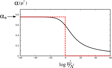
Figure 1: Two-loop running coupling (solid curve) compared with the approximate form in Eq. (8) (dashed line) in the case of SU(3) gauge theory with $12$ massless fundamental fermions.

In the figure, the two-loop running coupling (and its approximated form) in the case of SU(3) gauge theory with $12$ massless fundamental fermion is plotted as an example. The solid curve represents the two-loop running coupling which are obtained from the following RGE for $\alpha(\mu^{2})\ \Big{(}=\frac{\bar{g}^{2}(\mu^{2})}{4\pi}\,\Big{)}$:

$$\mu\frac{d}{d\mu}\alpha(\mu^{2})=\beta(\alpha(\mu^{2}))=-b\alpha^{2}(\mu^{2})-c\alpha^{3}(\mu^{2}),$$ (4)

where

$$b=\frac{1}{6\pi}\left(11N_{c}-2N_{f}\right),\quad c=\frac{1}{24\pi^{2}}\left(34N_{c}^{2}-10N_{c}N_{f}-3\frac{N_{c}^{2}-1}{N_{c}}N_{f}\right).$$ (5)

$\alpha_{\ast}$ is the value of the running coupling at the IRFP which is determined as

$$\alpha_{\ast}=-\frac{\ b\ }{\ c\ }.$$ (6)

Values of $\alpha_{\ast}$ in the case of SU(3) gauge theories with various number of fundamental fermion (in the conformal window) are shown in Table 1.

$N_{f}$	12	13	14	15	16
$\alpha_{\ast}$	0.75	0.47	0.28	0.14	0.042
$\gamma_{m}^{\ast}$	0.80	0.36	0.20	0.095	0.027

Table 1: Values of $\alpha_{\ast}$ and also listed are the corresponding $\gamma_{m}^{\ast}$ for SU(3) gauge theory with fundamental fermions in the conformal window to be given by Eq.(28).

$\Lambda$ which appears in Fig. 1 is a renormalization group invariant scale, $\Lambda=\mu\,\exp\left(-\int^{\alpha(\mu)}\frac{d\alpha}{\beta(\alpha)}\right)$, the two-loop analogue of $\Lambda_{\rm QCD}$ of the ordinary QCD, which is taken as atw

$$\Lambda\ \equiv\ \mu\ \exp\left[-\frac{1}{b\ \alpha_{\ast}}\log\left(\frac{\alpha_{\ast}-\alpha(\mu^{2})}{\alpha(\mu^{2})}\right)-\frac{1}{b\ \alpha(\mu^{2})}\right],\quad\alpha(\Lambda^{2})\simeq 0.78\,\alpha_{*},$$ (7)

in such a way that the scale $\Lambda$ plays the role of the “UV cutoff ” where the infrared conformality we are interested in terminates, i.e., $\alpha(\mu^{2})\sim{\rm const}(\simeq\alpha_{*})$ for $\mu^{2}<\Lambda^{2}$, while $\alpha(\mu^{2})\sim 1/\log(\mu^{2}/\Lambda^{2})$ for $\mu^{2}>\Lambda^{2}$ as in the usual asymptotically free theory. Actually in the walking technicolor, $\Lambda$ is taken to be of order of (or even larger than) the UV scale $\Lambda_{\rm ETC}$ (“ETC scale”) where the technicolor theory no longer makes sense as it stands and is actually converted into a more fundamental theory such as the Extended Technicolor (ETC).

In this paper we use the following form of the running coupling as an approximation of the two-loop running coupling (dashed line in Fig. 1) :

$$\alpha(\mu^{2})=\frac{{\bar{g}}^{2}(\mu^{2})}{4\pi}=\alpha_{\ast}\ \theta(\Lambda^{2}-\mu^{2}).$$ (8)

In this approximation the coupling takes the constant value $\alpha_{\ast}$ (the value at the IR fixed point) below the scale $\Lambda$ and entirely vanishes in the energy region above this scale. Therefore, the physical picture of the large $N_{f}$ QCD with this approximation is the same as that in constant coupling gauge theory with UV cutoff $\Lambda$ which was extensively studied long time ago Maskawa:1975hx ; Fukuda:1976zb ; Miransky:1984ef . We note that it is possible, at least numerically, to solve the SD equation without this approximation for the two-loop running coupling. However, we adopt this simplification so that we can analytically study the solution of the SD equation to a certain extent.

II.1 SD equation

Let us first write down the SD equation for $SU(N_{c})$ gauge theory with fundamental fermions:

$$iS_{F}^{-1}(p)\ =\ \hbox to0.0pt{\hbox to5.03125pt{\hfil/\hfil}\hss}p-m_{0}+\int\frac{d^{4}k}{i(2\pi)^{4}}\ C_{2}\,\bar{g}^{2}((p-k)^{2})\ \frac{1}{(p-k)^{2}}\left(g_{\mu\nu}-\frac{(p-k)_{\mu}(p-k)_{\nu}}{(p-k)^{2}}\right)\gamma^{\mu}\ iS_{F}(k)\ \gamma^{\nu}.$$ (9)

Here, $\ iS_{F}^{-1}\equiv A(p^{2})\hbox to0.0pt{\hbox to5.03125pt{\hfil/\hfil}\hss}p-B(p^{2})$ is the full fermion propagator, $\ C_{2}=\frac{N^{2}_{c}-1}{2N_{c}}$ is the quadratic Casimir, and $\ \bar{g}((p-q)^{2})$ is the running coupling constant. In the above expression, we took the Landau gauge, and adopted the improved ladder approximation, in which the full gauge boson propagator is replaced by the bare one and the full vertex function is replaced by a simple $\gamma^{\mu}$-type vertex with the running coupling constant associated with it. From this equation, we obtain the following two independent equations:

$$A(p^{2}) = 1+\int\frac{d^{4}k}{(2\pi)^{4}}\ \frac{C_{2}\,\bar{g}^{2}((p-k)^{2})}{k^{2}A(k^{2})^{2}+B(k^{2})^{2}}A(k^{2})\left[\frac{(p\cdot k)}{p^{2}(p-k)^{2}}+2\frac{\left\{p\cdot(p-k)\right\}\left\{k\cdot(p-k)\right\}}{p^{2}(p-k)^{4}}\right],$$ (10)

$$B(p^{2}) = m_{0}+\int\frac{d^{4}k}{(2\pi)^{4}}\ \frac{3\,C_{2}\,\bar{g}^{2}((p-k)^{2})}{k^{2}A(k^{2})^{2}+B(k^{2})^{2}}\ \frac{B(k^{2})}{(p-k)^{2}}.$$ (11)

These are coupled equations for $A(p^{2})$ and $B(p^{2})$ written in Euclidean momentum space. (Note that we have dropped the subscript “$E$” for Euclidean momentum variables.)

To further simplify the SD equation, we adopt a simplified form for the argument of the running coupling, ${\bar{g}}^{2}((p-k)^{2})$: we take it to be a function of only $p^{2}$ and $k^{2}$ instead of $(p-k)^{2}$. With this simplification, it becomes possible to carry out the angular integration (in the momentum space), then the SD equation becomes an equation for a single variable $x\equiv p_{E}^{2}$. Also, in this case, $A(x)=1$ is obtained from Eq. (10). Therefore, the SD equation becomes a single integral equation for the mass function $\Sigma(x)(\equiv B(x)/A(x)=B(x))$.

For the analytical study we adopt a practically simple ansatz for the running coupling: Miransky:1983vj

$${\bar{g}}^{2}((p-k)^{2})\Rightarrow{\bar{g}}^{2}(max\{p^{2},k^{2}\})\,.$$ (12)

Then the ladder SD equation with Eq.(8) reads:

$$\Sigma(x)=m_{0}+\alpha_{*}\frac{3C_{2}}{4\pi}\int_{0}^{\Lambda^{2}}dy\,\frac{1}{max\{x,y\}}\,\,\frac{\Sigma(y)}{y+\Sigma^{2}(y)}\,,$$ (13)

which can readily be converted into an equivalent (nonlinear) differential equation with boundary conditions Fukuda:1976zb :

$$\left(x\Sigma(x)\right)^{\prime\prime}+\alpha_{\ast}\frac{3C_{2}}{4\pi}\frac{\Sigma(x)}{x+\Sigma(x)^{2}} = 0,$$ (14)

$$\lim_{x\rightarrow 0}x^{2}\Sigma(x)^{\prime} = 0,$$ (15)

$$\left.\left(x\Sigma(x)\right)^{\prime}\right|_{x=\Lambda^{2}} = m_{0}.$$ (16)

We may further simplify Eq. (14) by replacing $\Sigma(x)$ in the denominator of the second term in the LHS by a constant, $m_{P}$, which is customarily defined by :

$$m_{P}\equiv\Sigma(x=m_{P}^{2}).$$ (17)

Then the SD equation reads: Fomin:1984tv

$$\left(x\Sigma(x)\right)^{\prime\prime}+\alpha_{\ast}\frac{3C_{2}}{4\pi}\frac{\Sigma(x)}{x+m_{P}^{2}} = 0.$$ (18)

We should note that it is known that the solution obtained from this linearized equation well approximates that obtained (by numerical calculation) from the equation without linearization. Later we shall show that particularly for the anomalous dimension there is a remarkable agreement between the analytical result obtained from the asymptotic solution of the linearized equation Eq.(18) and the numerical one from the full nonlinear integral SD equation under a slightly different ansatz for the argument of the running coupling (to be mentioned later).

$m_{P}$ defined in Eq. (17) is often called the “pole mass”, though of course $m_{P}$ is not the real pole mass (remember that $x$ is the Euclidean momentum square). Still, $m_{P}$ is useful quantity for the investigation of the hyperscaling relation since it is known, from the study with the Bethe-Salpeter equation Harada:2003dc , that $m_{P}$ is proportional to meson masses. Therefore, in this paper, we use $m_{P}$ which is obtained from the solution of the SD equation as low-energy physical quantity which appears in the hyperscaling relation.

II.2 Leading correction to the hyperscaling relation

Before we proceed to the investigation of the solution of the SD equation to derive the relation between $m_{P}$ and $m_{0}$, we note that it is known Maskawa:1975hx that there is a critical value of $\alpha_{\ast}$, $\alpha_{\rm cr}(\neq 0)$, such that spontaneous symmetry breaking solution ($\Sigma(x)\neq 0$) which satisfies Eqs. (18), (15) and (16) for the chiral limit $m_{0}=m_{0}(\Lambda)\equiv 0$ does not exists for

$$\alpha_{\ast}\leq\alpha_{\rm cr},$$ (19)

where Fukuda:1976zb

$$\alpha_{\rm cr}=\frac{\pi}{3C_{2}}\,=\frac{\pi}{4}\,\,(N_{c}=3)\,.$$ (20)

Namely, a nontrivial solution ($\Sigma(x)\neq 0$) for $\alpha<\alpha_{\rm cr}$ is the explicit breaking solution which exists only for $m_{0}=m_{0}(\Lambda)\neq 0$. Then the pole mass $m_{P}$ is nothing but a renormalized mass (“current mass”) $m_{R}$:

$$m_{P}=m_{R}=Z_{m}^{-1}\,m_{0},$$ (21)

where $m_{R}=m_{R}(\mu=m_{P})$, and $Z_{m}=Z_{m}\left(\frac{\mu}{\Lambda}\right)|_{\mu=m_{P}}$ is the mass renormalization constant. This means that, in the chiral limit $m_{R}=0$, there is no mass gap (dynamically generated mass) $m_{D}=0$, and therefore the IRFP of the theory is exact for $\alpha_{\ast}<\alpha_{\rm cr}$. This is exactly the region in which one expects that the hyperscaling relation should be satisfied. Therefore, in the rest of this section, we concentrate on studying the SD equation in the region of $\alpha_{\ast}<\alpha_{\rm cr}$, or equivalently (through the relation in Eq. (6)) $N_{f}^{\rm AF}\geq N_{f}\geq N_{f}^{\rm cr}$ (conformal window), where $N_{f}^{\rm AF}=16.5$ and $N_{f}^{\rm cr}\simeq 11.9$ for $N_{c}=3$.

A solution of Eq. (18) which satisfies boundary condition Eq. (15) can be expressed in terms of the hypergeometric function as Fomin:1984tv

$$\Sigma(x)\,=\,\xi\,m_{P}\,F\left(\frac{1+\omega}{2},\frac{1-\omega}{2},2,-\frac{x}{m_{P}^{2}}\right),$$ (22)

where

$$\omega\equiv\sqrt{1-\frac{\alpha_{\ast}}{\alpha_{\rm cr}}}.$$ (23)

$\xi$ is a numerical coefficient which is determined from the definition of $m_{P}$ in Eq. (17):

$$\xi^{-1}=F\left(\frac{1+\omega}{2},\frac{1-\omega}{2},2,-1\right).$$ (24)

In the limit of $x\gg m_{P}^{2}$, the solution can be expanded as

$$\Sigma(x)\,\simeq\,\xi\,m_{P}\,\left[\ \frac{\Gamma(\omega)}{\Gamma(\frac{\omega+1}{2})\,\Gamma(\frac{\omega+3}{2})}\left(\frac{x}{m_{P}^{2}}\right)^{\frac{\omega-1}{2}}\ +\ \ (\omega\leftrightarrow-\omega)\ \right].$$ (25)

By inserting the above expression of $\Sigma(x)$ into the remaining boundary condition in Eq. (16), we obtain the following relation between $m_{P}$ and $m_{0}$:

$$m_{0}\,=\,\xi\,m_{P}\,\left[\ \frac{\Gamma(\omega)}{\Gamma(\frac{\omega+1}{2})^{2}}\left(\frac{\Lambda^{2}}{m_{P}^{2}}\right)^{\frac{\omega-1}{2}}\ +\ \ (\omega\leftrightarrow-\omega)\ \right].$$ (26)

From this we have the mass renormalization constant $Z_{m}$ in Eq.(21) as

$$Z_{m}\equiv\frac{m_{0}}{m_{R}}=\frac{m_{0}}{m_{P}}=\,\xi\,\left[\ \frac{\Gamma(\omega)}{\Gamma(\frac{\omega+1}{2})^{2}}\left(\frac{\Lambda^{2}}{m_{P}^{2}}\right)^{\frac{\omega-1}{2}}\ +\ \ (\omega\leftrightarrow-\omega)\ \right]\,,$$ (27)

where we note again $m_{P}=m_{R}$ in the conformal window.

Then we can obtain the mass anomalous dimension at IRFP, $\gamma_{m}^{\ast}$, as

$$\gamma_{m}^{\ast}\ =\lim_{m_{P}/\Lambda\rightarrow 0}\frac{\partial\log Z_{m}}{\partial\log(m_{P}/\Lambda)}=\ 1-\omega\ \left(=\ 1-\sqrt{1-\frac{\alpha_{\ast}}{\alpha_{\rm cr}}}\ \right)\,,$$ (28)

where the limit is taken as $m_{P}\rightarrow 0$ with $\Lambda$ fixed. In Table 1, we show values of $\gamma_{m}^{\ast}$, which can be calculated from the above expression combined with Eqs. (5), (6) and (20), in the case of SU(3) gauge theory with various numbers of fundamental fermion in the conformal window.

It should be noted that this $\gamma_{m}^{*}$ at IRFP is actually the same as the anomalous dimension in the UV limit ($\Lambda\rightarrow\infty$ with $m_{P}$ fixed) $\gamma_{m}^{(\rm UV)}\equiv\lim_{\Lambda/m_{P}\rightarrow\infty}\frac{\partial\log Z_{m}}{\partial\log(m_{P}/\Lambda)}=1-\omega$ Bardeen:1985sm . $\gamma_{m}^{(\rm UV)}$ is the quantity relevant to the walking technicolor with $\gamma_{m}^{(\rm UV)}=1$ (the value at (pseudo-) UV fixed point in the broken phase $\alpha_{*}>\alpha_{\rm cr}$ in the chiral limit $m_{R}=0$: $m_{P}=m_{D}$) wtc1 : The technifermion condensate $\langle\bar{\psi}\psi\rangle|_{\Lambda}$ at the UV scale $\Lambda=\Lambda_{\rm ETC}(>10^{3}{\rm TeV})\gg\mu\,(={\cal O}(m_{P})={\cal O}({\rm TeV})$) is enhanced by $\gamma_{m}^{(\rm UV)}=1$ as $\langle\bar{\psi}\psi\rangle|_{\Lambda}=Z_{m}^{-1}\langle\bar{\psi}\psi\rangle|_{\mu}$ with $Z_{m}^{-1}=(\Lambda/\mu)^{\gamma_{m}^{(\rm UV)}}=(\Lambda/\mu)^{1}\gg 1$.

By using this $\gamma_{m}^{*}$, we can rewrite the expression in Eq. (26) in terms of $\gamma_{m}^{\ast}$:

$$\frac{m_{0}}{\Lambda}\ =\ \xi\,\left[\ \frac{\Gamma(1-\gamma_{m}^{\ast})}{\Gamma(\frac{2-\gamma_{\ast}}{2})^{2}}\left(\frac{m_{P}}{\Lambda}\right)^{1+\gamma_{m}^{\ast}}+\ \frac{\Gamma(-1+\gamma_{m}^{\ast})}{\Gamma(\frac{\gamma_{\ast}}{2})^{2}}\left(\frac{m_{P}}{\Lambda}\right)^{3-\gamma_{m}^{\ast}}\ \right].$$ (29)

This is the expression which should be compared with the hyperscaling relation in Eq. (1). It is obvious that if we drop the second term in the RHS of Eq. (29), it reduces to the hyperscaling relation Miransky . Therefore, the second term should be identified as the leading correction to the hyperscaling relation.

To see the significance of the correction term, in Fig. 2, we plot ratios of the second term to the first term in the RHS of Eq. (29) as functions of $m_{P}/\Lambda$ for various values of $\gamma_{m}^{\ast}$ in the range of $0\leq\gamma_{m}^{\ast}\leq 1.0$, which corresponds to $N_{f}^{\rm AF}\geq N_{f}\geq N_{f}^{\rm cr}$.

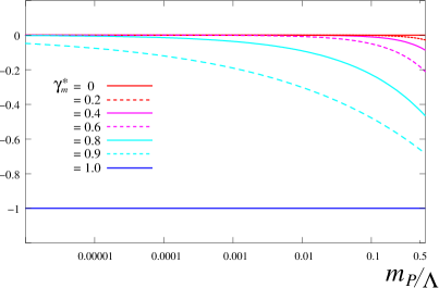
Figure 2: Ratios of the second term to the first term in the RHS of Eq. (29) as functions of $m_{P}/\Lambda$ for various values of $\gamma_{m}^{\ast}$.

When $m_{P}$ is much smaller than $\Lambda$, (except in the case of $\gamma_{m}^{\ast}=1.0$) the effect of the second term is very small since in the range of $0<\gamma_{m}^{\ast}<1.0$, the power of $(m_{P}/\Lambda)$ in the second term is always greater than that in the first term. This is reasonable considering the fact that small $m_{P}$ (or equivalently, small $m_{0}$) means small mass deformation. Another limit in which Eq. (29) approximates well the hyperscaling is $\gamma_{m}^{\ast}\rightarrow 0$. In this limit, the coefficient of the second term goes to $0$ while that of the first term goes to $1$. Also, the power suppression of the second term becomes strong in this limit as well. However, we should remember that phenomenologically motivated theories have large $\gamma_{m}^{\ast}$. In the limit of $\gamma_{m}^{\ast}\rightarrow 1$, the power of $(m_{P}/\Lambda)$, as well as coefficients of the two terms asymptote to the same values. Therefore, we have to take the second term seriously when we study the anomalous dimension of the candidate theories for viable walking technicolor models with $\gamma_{m}\simeq 1$ through the hyperscaling relation from the numerical data on the lattice.

For checking the reliability of our ansatz Eq.(12) and the linearization of the differential equation, as well as the asymptotic expansion Eq.(25), we show in Fig. 3 the log-scale plot of $m_{0}-m_{P}$ in Eq.(29) for $N_{f}=12$ in comparison with that obtained by directly solving numerically the full nonlinear SD equation with more natural (angle-averaged) ansatz:

$${\bar{g}}^{2}((p-k)^{2})\Rightarrow{\bar{g}}^{2}(p^{2}+k^{2})\,.$$ (30)

The SD equation in this case with Eq.(8) reads:

$$\Sigma(x)=m_{0}+\alpha_{*}\frac{3C_{2}}{4\pi}\int_{0}^{\Lambda^{2}-x}dy\,\frac{1}{max\{x,y\}}\,\,\frac{\Sigma(y)}{y+\Sigma^{2}(y)}\,,$$ (31)

which differs from Eq.(13) by $\Lambda^{2}-x$ in the UV end of the integral. The slope in Fig.(3) corresponds to $\gamma_{m}+1$. The agreement is remarkable, irrespectively of the different ansatz and the additional approximations.

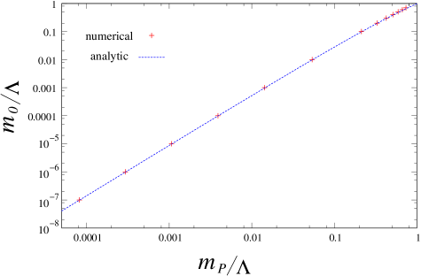
Figure 3: Analytical asymptotic solution of the linearized SD equation vs. numerical solution of the full nonlinear one (for $N_{f}=12$). Analytic result (blue dotted line) is the plot of Eq. (29) which is from the asymptotic expansion of the linearized SD equation Eq.(18) with the ansatz Eq.(12), while the numerical one (denoted by red plus) is that of the solution of the full nonlinear integral SD equation Eq.(31) with ansatz Eq.(30).

II.3 Effective anomalous dimension

In the literature, the hyperscaling relation is often used as a tool to judge whether a theory is infrared conformal or not. However, the importance of the corrections to the hyperscaling relation due to the mass deformation are often underestimated, or even completely neglected. This is not surprising because, in practical situations, it is very difficult to notice that data (for example, hadron mass, $M_{H}$, obtained from lattice simulations with various values of input $m_{0}a$) need to be fitted by a function with correction term. Even in the situation that the correction term is not very small compared to the leading term, data could be easily fitted by a simple function of a form $m_{0}\sim M_{H}^{1+\gamma}$ unless data are taken in a wide range of $m_{0}$ (or, equivalently, $M_{H}$). Especially when the data are associated with, say, a few percent of error bars, it is very possible that one succeeds in fitting the data with a function of a form $m_{0}\sim M_{H}^{1+\gamma}$. However, the best-fit value of $\gamma$ obtained by this fitting must be numerically different from the actual mass anomalous dimension at the IRFP. To make the difference clear, we introduce effective mass anomalous dimension, $\gamma_{m}^{\rm eff}$, which is defined as the value of $\gamma$ one obtains as a best-fit value when one forces to do fitting by using a fit-function which has a form of hyperscaling relation. Since the significance of the correction term is different for different values of $M_{H}$, the value of $\gamma_{m}^{\rm eff}$ should change depending on the range of $M_{H}$ one uses for fitting to obtain it.

In the framework of the SD equation with the improved ladder approximation, we can identify $\gamma_{m}^{\rm eff}$ as $\gamma_{m}=\gamma_{m}(\mu/\Lambda)|_{\mu=m_{P}}$ obtained from Eq.(27) with Eq.(28) (or equivalently Eq. (29)):

$$\gamma_{m}^{\rm eff}=\gamma_{m} = \frac{\partial\log Z_{m}}{\partial\log(m_{P}/\Lambda)}$$ (32)

$$= \frac{\partial}{\partial\log(m_{P}/\Lambda)}\log{\left(\xi\,\left[\ \frac{\Gamma(1-\gamma_{\ast})}{\Gamma(\frac{2-\gamma_{\ast}}{2})^{2}}\left(\frac{m_{P}}{\Lambda}\right)^{\gamma_{m}^{\ast}}+\ \frac{\Gamma(-1+\gamma_{\ast})}{\Gamma(\frac{\gamma_{\ast}}{2})^{2}}\left(\frac{m_{P}}{\Lambda}\right)^{2-\gamma_{m}^{\ast}}\ \right]\right)}$$ (33)

It is obvious that were it not for the second term, $\gamma_{m}^{\rm eff}$ would coincide with $\gamma_{m}^{*}$. Note again that the significance of the correction term is different for different values of $m_{P}$. Therefore, the effective mass anomalous dimension becomes a function of $m_{P}$. In Fig. 4, $\gamma_{m}^{\rm eff}$ for SU(3) gauge theories with 12, 13, 14, 15 and 16 fundamental fermions are plotted as a function of $m_{P}$. For the purpose of making it easier to see the deviation of the effective mass anomalous dimension from the value at the IRFP, we also plot $\gamma_{m}^{\rm eff}/\gamma_{m}^{\ast}$ in Fig. 5.

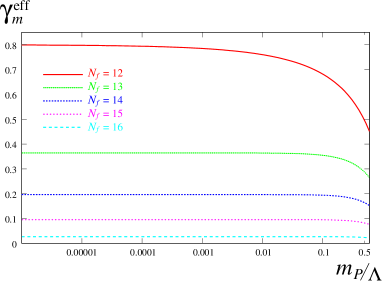
Figure 4: Effective mass anomalous dimension as a function of $m_{P}/\Lambda$ for SU(3) gauge theories with 12, 13, 14, 15 and 16 fundamental fermions.

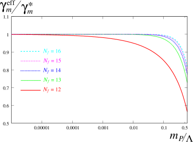
Figure 5: Effective mass anomalous dimension which is normalized by the value of it at the IRFP as a function of $m_{P}/\Lambda$ for SU(3) gauge theories with 12, 13, 14, 15 and 16 fundamental fermions.

From these figures, as we expected, we see that the deviation between $\gamma_{m}^{\rm eff}$ and $\gamma_{m}^{\ast}$ becomes more significant in larger $m_{P}/\Lambda$ region. We can also see that the deviation of the effective mass anomalous dimension is larger for smaller $N_{f}$ (or, in other words, for $N_{f}$ closer to $N_{f}^{\rm cr}\simeq 11.9$). This is also expected from the discussion below Eq. (29) because smaller $N_{f}$ means larger $\gamma_{m}^{\ast}$, with which the correction term to the hyperscaling relation becomes important. As we mentioned earlier, phenomenologically interesting theory is the one with large mass anomalous dimension. Therefore, it is important to keep this effect of correction term to the hyperscaling relation in mind when one study such theories.

III Effect of the corrections on the finite-size hyperscaling

So far we have concentrated on the study of the hyperscaling relation in the infinite space-time. However, since the lattice simulations are done in a finite space-time, the hyperscaling relation in a form of Eq. (2) are used more often. Therefore, it is important to study the effect of correction due to mass deformation on the finite-size hyperscaling relation. For the purpose of studying the finite-size hyperscaling relation, we formulate the SD equation in a finite space-time with the periodic boundary condition. By numerically solving it for various values of input parameters $(\hat{m}_{0},\hat{L})$, mass deformation effects on the finite-size hyperscaling relation is studied in large $N_{f}$ QCD.

III.1 SD equation in a finite space-time

To formulate the SD equation in a finite space-time, we start from the SD equation in the infinite space-time in Eqs. (10) and (11). To put these equations in a finite space-time, all one needs to do is to replace the continuum momentum variables by the discrete ones:

$$p_{i}\rightarrow\tilde{p}_{i}=\frac{2\pi n_{i}}{L},\ \ \ \ (n_{i}\in\mathbb{N}),$$ (34)

where, $p_{i}$ is the $i$-th component of the momentum variable. We adopted the periodic boundary condition for all directions, though it is easy to implement the anti-periodic boundary condition. We also assumed that the size of all space-time directions are the same. It is also straightforward to introduce different sizes for spacial and temporal directions. However, we took the same length for every direction just for simplicity. $n_{i}$’s are integers which label discrete momentum variables. With this replacement of the momentum variables, the SD equation in Eqs. (10) and (11) turn into the following form:

$$\tilde{A}(\tilde{p}) = 1+\frac{1}{L^{4}}\sum_{m_{0,1,2,3}}\frac{C_{2}\,\bar{g}^{2}((\tilde{p}-\tilde{k})^{2})}{\tilde{k}^{2}\tilde{A}(\tilde{k})^{2}+\tilde{B}(\tilde{k})^{2}}\tilde{A}(\tilde{k})\left[\frac{(\tilde{p}\cdot\tilde{k})}{\tilde{p}^{2}(\tilde{p}-\tilde{k})^{2}}+2\frac{\left\{\tilde{p}\cdot(\tilde{p}-\tilde{k})\right\}\left\{\tilde{k}\cdot(\tilde{p}-\tilde{k})\right\}}{\tilde{p}^{2}(\tilde{p}-\tilde{k})^{4}}\right],$$ (35)

$$\tilde{B}(\tilde{p}) = m_{0}+\frac{1}{L^{4}}\sum_{m_{0,1,2,3}}\frac{3\,C_{2}\,\bar{g}^{2}((\tilde{p}-\tilde{k})^{2})}{\tilde{k}^{2}\tilde{A}(\tilde{k})^{2}+\tilde{B}(\tilde{k})^{2}}\ \frac{\tilde{B}(\tilde{k})}{(\tilde{p}-\tilde{k})^{2}},$$ (36)

where

$$\tilde{p}=\frac{2\pi}{L}\left(\begin{array}[]{c}n_{0}\\ n_{1}\\ n_{2}\\ n_{3}\\ \end{array}\right),\ \ \ \tilde{k}=\frac{2\pi}{L}\left(\begin{array}[]{c}m_{0}\\ m_{1}\\ m_{2}\\ m_{3}\\ \end{array}\right).$$ (45)

Here, $n_{i}$ and $m_{i}$ are integers, though we should note that the SD equation is not defined at $\tilde{p}=0$ since one of the two independent equations is derived by requiring coefficients of $\hbox to0.0pt{\hbox to5.03125pt{\hfil/\hfil}\hss}p$ in LHS and RHS are the same in Eq. (9). In the above expressions, $A(p^{2})$ and $B(p^{2})$ were replaced by $\tilde{A}(\tilde{p})$ and $\tilde{B}(\tilde{p})$. This is because they are no longer functions of momentum-squared since the rotational symmetry is broken (except some residual discrete rotational symmetry) due to the hyper-cubic shape of the finite-size space-time. However, at the practical level, the effect of such rotational-symmetry violation is negligible as far as $L$ is taken large enough compared to the scale of relevant physics. This is true in the case of the current study. We first numerically solve, by using iteration method, Eqs. (35) and (36) as coupled equations for $\tilde{A}(\tilde{p})$ and $\tilde{B}(\tilde{p})$. Then, to obtain the value of $m_{P}$ (see Eq. (17)), we plot $\tilde{\Sigma}(\tilde{p})\equiv\tilde{B}(\tilde{p})/\tilde{A}(\tilde{p})$ as a function of $\tilde{p}^{2}$. There are always multiple $\tilde{p}$’s which give the same value of $\tilde{p}^{2}$, and those do not necessarily give a degenerate value of $\tilde{\Sigma}$ unless those are related by the residual discrete rotational symmetry. However, we confirmed that such differences are negligible in the region where $m_{P}$ is determined. We should also note that, when we estimate the value of $m_{P}$ from Eq. (17), we used a function which is obtained by interpolating $\tilde{\Sigma}(\tilde{p})$ in momentum space. However, we never did extrapolation to the scale below $2\pi/L$ since there is no reliable information below that scale. Therefore, we obtain data only when the value of $m_{P}^{2}$ is greater $(2\pi/L)^{2}$.

III.2 Finite-size hyperscaling and its corrections

In this subsection, by numerically solving the finite-volume SD equation formulated in the previous subsection, we generate data of $m_{P}$ for various sets of input parameters $(L\Lambda,m_{0}/\Lambda)$. We take SU(3) gauge theory with 12 fundamental fermion as an example here. Then, by using those generated data, we do the analysis based on the finite-size hyperscaling in Eq. (2). This is a kind of “simulation” of the practical situation we often encounter when we study a theory by using data obtained from lattice simulations. An interesting point about doing hyperscaling analysis using data generated by the SD equation is that we know that the SU(3) gauge theory with 12 fundamental fermions, in the framework of the SD equation, is the infrared conformal theory, and we also know the value of the mass anomalous dimension at the IRFP, which is estimated as $\gamma_{m}^{\ast}\simeq 0.80$ in this case. (See Table 1.) Therefore, we clearly see how the finite-size hyperscaling is violated due to the effect of the mass deformation.

In Fig. 6, we plot the values of $m_{P}/\Lambda$ (horizontal axis) for various values of $m_{0}/\Lambda$ (vertical axis) and $L\Lambda$ (indicated by different symbols).

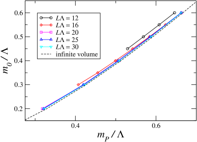
Figure 6: Values of $m_{P}/\Lambda$ (horizontal axis) for various values of $m_{0}/\Lambda$ (vertical axis) and $L\Lambda$ (indicated by different symbols) for SU(3) gauge theory with 12 fundamental fermions. Dashed curve is $m_{P}$ as a function of $m_{0}$ which is obtained from the numerical solution of the SD equation in the infinite space-time (Eqs. (10) and (11)).

When we solved the finite volume SD equation, we adopted an angle averaged form (as in Eq. (30)) for the argument of the running coupling. As we explained in the previous section, this is the procedure which is needed to make the angular integration (in momentum space) possible in the case of infinite-volume SD equation, and it is actually not needed for finite-volume SD equation since we numerically solve them by iteration without doing angular integration. However, for the purpose of putting finite- and infinite-volume SD equations on the same ground, we adopted angle averaged argument for finite-volume SD equation as well. We note that when we adopt the angle-averaged form for the argument of the running coupling, summations in the finite-volume SD equation are restricted in the range of $\tilde{p}^{2}+\tilde{k}^{2}\leq\Lambda^{2}$.

In Fig. 6, in each $L\Lambda$, one notices that data are plotted in the range of $m_{P}/\Lambda$ which is larger than a certain value. This lower limit comes from the IR cutoff effect which was explained at the end of the previous subsection. Dashed curve in the figure is $m_{P}$ as a function of $m_{0}$ which is obtained from the numerical solution of the SD equation in the infinite space-time (Eqs. (10) and (11) with the ansatz Eq.(30) and Eq.(8)). In the figure we see that data for $L\Lambda=20,25,30$ are almost degenerate, and take values close to the dashed curve for the infinite space-time. This means that $L\Lambda=20$ is large enough that the finite-size effect is negligible for the determination of $m_{P}$ in this mass range.

Now, let us do the finite-size hyperscaling analysis by using data shown in Fig. 6. In Fig. 7, we plot the values of $m_{P}L$ as a function of $x\equiv L\Lambda(m_{0}/\Lambda)^{1/(1+\gamma)}$ for $\gamma=0.2,0.4,0.5,0.6,0.7$ and $0.8$. If the theory is infrared conformal, and if the effect of the mass deformation is negligible, this kind of plot should show good alignment of data when input value of $\gamma$ is chosen to be $\gamma_{m}^{*}$, the value of mass anomalous dimension at the IRFP. Here, we know that, in the framework of the SD equation, the theory is infrared conformal, and the value of the mass anomalous dimension at the IRFP is $\gamma_{m}^{\ast}\simeq 0.8$. However, plot in Fig. 7 shows no alignment for $\gamma=0.8$, instead, data are well aligned for $\gamma=0.5$ and $0.6$. This suggests that the effect of the correction to the hyperscaling relation due to the large mass deformation appears also in the case of finite-size hyperscaling relation. Note that data we used here are in the range of $m_{P}/\Lambda\gtrsim 0.3$. In that range, from Fig. 4, we see that the effective anomalous dimension takes the value $\gamma_{m}^{\rm eff}=0.5\sim 0.6$. This is the reason why the data show good finite-size hyperscaling with input value of $\gamma_{m}^{\rm eff}=\gamma=0.5\sim 0.6$. We have done the same analysis for SU(3) gauge theory with $N_{f}=14$ and $16$, and found similar results.

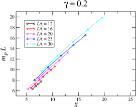
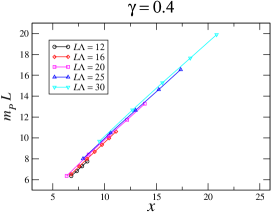
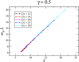
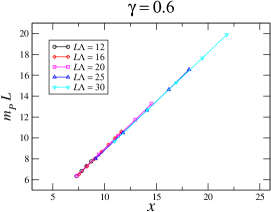
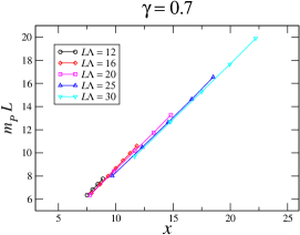
Figure 7: Values of $m_{P}L$ obtained from the finite-volume SD equation as a function of $x\equiv L\Lambda(m_{0}/\Lambda)^{1/(1+\gamma)}$ for $\gamma=0.2,0.4,0.5,0.6,0.7$ and $0.8$ in SU(3) gauge theory with 12 fundamental fermions. Data for $L\Lambda=12,16,20,25$ and $30$ are plotted as different symbols.

It is interesting to ask whether there is a function which can be fitted to all the data shown in Fig. 6. We tried the following form of fit function, and found that it can be globally fitted to all the data fairly well:

$$m_{0}(L,m_{P})=\left[Am_{P}(1+Bm_{P}^{2-2\gamma})^{1/(1+\gamma)}+\frac{C}{L}\right]^{1+\gamma}.$$ (46)

Here, $A,B,C$ and $\gamma$ are fit parameters, and it is understood that all the dimensionful quantities are normalized by $\Lambda$. This fit function is similar to the form of finite-size hyperscaling relatinon in Eq. (2): When one takes $B=0$, $Lm_{P}$ is expressed by a function of $x=Lm_{0}^{1/(1+\gamma)}$. The term proportional to $B$ represents the effect of mass correction to the hyperscaling relation. The best-fit values we obtained for fit parameters are: $A=1.52,B=-0.512,C=0.323$ and $\gamma=0.794$. It is remarkable that we obtained value of $\gamma$ which is quite close to the value of $\gamma_{m}^{\ast}=0.8$. For comparison, we also did fitting with fixing $B=0$, and found that the best-fit value of $\gamma=0.52$. This is consistent with Fig. 7, in which it was shown that finite-size scaling (without correction term) is approximately satisfied when $\gamma=0.5\sim 0.6$. Of course, the power of the second term in the RHS of Eq. (46), namely $2-2\gamma$, is specific to the ladder SD analysis, though it is worth trying to do fitting lattice data with using the above fit function. One could also make the power of the second term in the RHS of Eq. (46) as free parameter. If the chi-square of the fitting significantly reduces by the inclusion of the correction term, or even if the chi-square does not change very much but the value of $\gamma$ significantly changes, it is very possible that the best-fit value of $\gamma$ which is obtained with correction term into consideration is close to the actual value of $\gamma_{m}^{\ast}$.

III.3 Violation of the hyperscaling relation in theories with spontaneous chiral symmetry breaking

Here, by the same procedure used in the previous subsection, we study the finite-size hyperscaling relation in theories with spontaneous chiral symmetry breaking. In the case of theories with spontaneous chiral symmetry breaking, mass gap exists even in the chiral limit, and therefore an IRFP is only approximate. Here, we show two examples: one is SU(3) gauge theory with $N_{f}=9$, and the other is that with $N_{f}=11$. The former is an example of a theory which is far away from the conformal window, in which the infrared conformality is expected to be largely violated. The latter is an example of a theory which resides close to the conformal window, and the breaking of the infrared conformality due to the spontaneous chiral symmetry breaking is expected to be small.

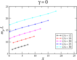
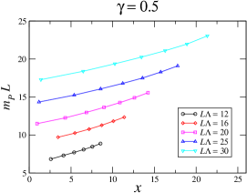
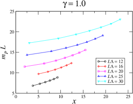
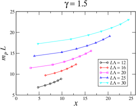
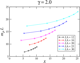
Figure 8: Values of $m_{P}L$ obtained from the finite-volume SD equation as a function of $x\equiv L\Lambda(m_{0}/\Lambda)^{1/(1+\gamma)}$ for $\gamma=0,0.5,1.0,1.5$ and $2.0$ in SU(3) gauge theory with 9 fundamental fermions. Data for $L\Lambda=12,16,20,25$ and $30$ are plotted as different symbols.

In Fig. 8, we show the plots of $m_{P}L$ obtained from the finite-volume SD equation in SU(3) gauge theory with 9 fundamental fermions as a function of $x\equiv L\Lambda(m_{0}/\Lambda)^{1/(1+\gamma)}$ for $\gamma=0,\,0.5,\,1.0,\,1.5$ and $2.0$. Data for $L\Lambda=12,16,20,25$ and $30$ are plotted as different symbols. As we expected, since the infrared conformality is largely broken due to the spontaneous chiral symmetry breaking, large violation of hyperscaling relation is observed. Note that the dynamically generated mass for $N_{f}=9$ is $m_{D}/\Lambda\simeq 0.58$, where $m_{D}$ is the value of $m_{P}$ obtained by the spontaneously broken solution of the ladder SD equation in the chiral limit $m_{0}\equiv 0$. ($m_{D}$ is estimated by the SD equations, Eq. (31), in the chiral limit $m_{0}=0$.) This is compared with the typical values in Fig. 8: $m_{P}/\Lambda=0.58-0.77$ for $L\Lambda=30$.

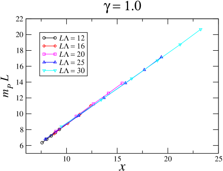
Figure 9: Values of $m_{P}L$ obtained from the finite-volume SD equation as a function of $x\equiv L\Lambda(m_{0}/\Lambda)^{1/(1+\gamma)}$ for $\gamma=1.0$ in SU(3) gauge theory with 11 fundamental fermions. Data for $L\Lambda=12,16,20,25$ and $30$ are plotted as different symbols.

On the other hand, a similar plot for SU(3) gauge theory with 11 fundamental fermions is given Fig. 9. We show the result for $\gamma=1.0$, with which we found data are best aligned each other. Again, as we expected, since the theory is close to the chiral restoration point, and the effect of the spontaneous chiral symmetry breaking is small, the violation of hyperscaling relation is small. Note that $m_{D}/\Lambda\simeq 0.05$ for $N_{f}=11$, while typical values of $m_{P}$ in Fig. 9 are $m_{P}/\Lambda=0.28-0.69\,(\gg m_{D}/\Lambda)$ for $L\Lambda=30$. Of course, one can see that there is a small amount of misalignment. However, let us imagine those were data obtained from lattice simulations, and each data point has, say, a few percent error bar, in which case, the data might look consistent with conformal hyperscaling. Therefore, when one obtained data which look consistent with conformal hyperscaling with a large mass anomalous dimension, there is a possibility that the theory is exactly the one the technicolor model favors, namely the dynamics with spontaneous chiral symmetry breaking at hierarchically small scale compared to $\Lambda$ with large anomalous dimension.

IV Summary and Discussion

In this paper, we studied corrections to the conformal hyperscaling relation by taking the example of SU(3) gauge theories with various number of fundamental fermion. From the analytical expression of the solution of the ladder SD equation, we identified the form of the leading correction to the hyperscaling relation. We found that the anomalous dimension, when identified through the hyperscaling relation neglecting these corrections (which we denoted as $\gamma_{m}^{\rm eff}$), tends to be lower than the real value at the fixed point.

We further studied finite-size hyperscaling relation through the ladder SD equation in a finite space-time with the periodic boundary condition. We found that the anomalous dimension, when identified through the finite-size hyperscaling relation neglecting the mass corrections as is often done in the lattice analyses, yields almost the same value as that in the case of the infinite space-time neglecting the mass correction, i.e., a lower value than $\gamma_{m}^{*}$. The introduction of the finite size of space-time should also break the infrared conformality, though we found that the correction to the hyperscaling relation due to the finite-volume effect seems to be negligible at least in the range of $L$ we studied in this paper. This can be seen from the fact that the finite-size hyperscaling relation is approximately satisfied with $\gamma_{m}^{\rm eff}$ which is obtained from the infinite-volume analysis. If $1/L$ correction were large, there must have been a visible violation of hyperscaling relation caused by it. The smallness of correction coming from finite-size effect can also be understood from the fact that a function with a form shown in Eq. (46), in which only mass correction is taken into account, can be fitted to all the data in Fig. 6 pretty well.

We also applied the finite-volume SD equation to the chiral-symmetry-breaking phase and found that when the theory is close to the critical point such that the dynamically generated mass is much smaller than the explicit breaking mass, the finite-size hyperscaling relation is still operative, with the mass corrections to the anomalous dimension being somewhat involved, however.

From a lattice simulation point of view, there are several things we can learn from the results of the present paper. When the input bare mass is not small enough, and data are not precise enough to find the mass correction, finite-size hyperscaling plot might give fairly good aligned picture with a value of the mass anomalous dimension which is much smaller than the value at the IRFP. If data are precise enough, one could notice misalignment of data which is caused by the fact that the value of $\gamma_{m}^{\rm eff}$ is different for different values of the meson mass $M$. However, if one didn’t know that the misalignment is fake coming from the correction term, one could draw conclusion that the theory is not infrared conformal, even though it actually is. As we mentioned at the end of the previous section, opposite could also happen, namely, even if a theory is actually in the chiral symmetry breaking phase, one could draw conclusion that it is infrared conformal especially when the amount of spontaneous chiral symmetry breaking is very small and/or data is not precise enough. Thus, careful attitude is important when one judges whether a theory is infrared conformal or not by using hyperscaling analysis. However, main message of our analysis is that if one observed a certain type of the finite-size hyperscaling relation (with some finite mass corrections), it already hints the remnant of the IR conformal theory no matter it may be in the broken phase (applicable to the walking technicolor) or the conformal window: It implies a new situation of the 4-dimensional non-Supersymmetric gauge theories and a new phenomenological application.

In this paper, we studied large $N_{f}$ QCD as a concrete example for the study of hyperscaling relation, though the extension to different number of color and different fermion representation is straightforward. This is because, in the context of the SD equation with the improved ladder approximation, $C_{2}\,\bar{g}^{2}$ appearing in the equation is the only quantity which differentiate different theories, and with the simplification of the running coupling adopted in the current study, this is proportional to $\alpha_{\ast}/\alpha_{\rm cr}$. Therefore the only relevant thing is how close the value of the running coupling at the IRFP is to the critical coupling.

It is also interesting to ask what is the best way of analyzing data to extract the correct picture. The SD equation gives us a nice playground to try to find an analysis method which works well for finding correct picture of a given theory since it can generate as many data as we like, and we know the “answer”, namely, whether the theory possesses an IRFP, and also the value of the mass anomalous dimension in that theory. We can try several different analysis methods with those generated data, and compare the results with the answer. By doing so, we can tell which analysis method produces the answer rather correctly. We tried fitting using the fit function shown in Eq. (46) as an example of such studies, and found that it works quite well extracting the true value of $\gamma_{m}^{\ast}$ of the theory. Of course, it is worth investigating further in this direction. Various different analysis methods should be studied for the purpose of finding a practical method which can extract a more correct picture from lattice data.

- (1) S. Weinberg, Phys. Rev. D 19, 1277 (1979); L. Susskind, ibid. D 20, 2619 (1979); see also S. Weinberg, Phys. Rev. D 13, 974 (1976).
- (2) See for reviews, e.g., E. Farhi and L. Susskind, Phys. Rept. 74, 277 (1981); C. T. Hill and E. H. Simmons, Phys. Rept. 381, 235 (2003) [Erratum-ibid. 390, 553 (2004)] [arXiv:hep-ph/0203079], and references therein.
- (3) K. Yamawaki, M. Bando, and K. Matumoto, Phys. Rev. Lett. 56, 1335 (1986); M. Bando, K. -i. Matumoto, and K. Yamawaki, Phys. Lett. B178 (1986) 308; M. Bando, T. Morozumi, H. So, and K. Yamawaki, Phys. Rev. Lett. 59, 389 (1987).
- (4) For similar discussion without notion of scale invariance and large mass anomalous dimension, see B. Holdom, Phys. Lett. B 150, 301 (1985); T. Akiba and T. Yanagida, Phys. Lett. B 169, 432 (1986); T.W. Appelquist, D. Karabali, and L.C.R. Wijewardhana, Phys. Rev. Lett. 57, 957 (1986).
- (5) K. D. Lane and M. V. Ramana, Phys. Rev. D 44, 2678 (1991).
- (6) W. E. Caswell, Phys. Rev. Lett. 33, 244 (1974).
- (7) T. Banks and A. Zaks, Nucl. Phys. B196, 189 (1982).
- (8) T. Appelquist, J. Terning, and L. C. R. Wijewardhana, Phys. Rev. Lett. 77, 1214 (1996); T. Appelquist, A. Ratnaweera, J. Terning, and L. C. R. Wijewardhana, Phys. Rev. D 58, 105017 (1998).
- (9) V. Miransky and K. Yamawaki, Phys. Rev. D 55, 5051 (1997); ibid. 56, E 3768 (1997).
- (10) D. B. Kaplan, J. W. Lee, D. T. Son, and M. A. Stephanov, Int. J. Mod. Phys. A 25, 422 (2010).
- (11) J. B. Kogut and D. K. Sinclair, Nucl. Phys. B295, 465 (1988).
- (12) Y. Iwasaki, K. Kanaya, S. Sakai, and T. Yoshie, Phys. Rev. Lett. 69, 21 (1992); Y. Iwasaki, K. Kanaya, S. Kaya, S. Sakai, and T. Yoshie, Phys. Rev. D69, 014507 (2004). [hep-lat/0309159].
- (13) F. R. Brown, H. Chen, N. H. Christ, Z. Dong, R. D. Mawhinney, W. Schaffer, and A. Vaccarino, Phys. Rev. D46, 5655-5670 (1992). [hep-lat/9206001].
- (14) P. H. Damgaard, U. M. Heller, A. Krasnitz, and P. Olesen, Phys. Lett. B400, 169-175 (1997). [hep-lat/9701008].
- (15) See, for example, T. Appelquist, G. T. Fleming, and E. T. Neil, Phys. Rev. Lett. 100, 171607 (2008) [Erratum-ibid. 102, 149902 (2009)] [arXiv:0712.0609 [hep-ph]]; Phys. Rev. D 79, 076010 (2009) [arXiv:0901.3766 [hep-ph]]; S. Catterall, J. Giedt, F. Sannino, and J. Schneible, JHEP 0811, 009 (2008) [arXiv:0807.0792 [hep-lat]]; A. J. Hietanen, K. Rummukainen, and K. Tuominen, Phys. Rev. D 80, 094504 (2009) [arXiv:0904.0864 [hep-lat]]; A. Deuzeman, M. P. Lombardo, and E. Pallante, Phys. Rev. D 82, 074503 (2010) [arXiv:0904.4662 [hep-ph]]; L. Del Debbio, B. Lucini, A. Patella, C. Pica, and A. Rago, Phys. Rev. D 80, 074507 (2009) [arXiv:0907.3896 [hep-lat]]; Z. Fodor, K. Holland, J. Kuti, D. Nogradi, and C. Schroeder, Phys. Lett. B 681, 353 (2009) [arXiv:0907.4562 [hep-lat]]; K. -i. Nagai, G. Carrillo-Ruiz, G. Koleva, and R. Lewis, Phys. Rev. D 80, 074508 (2009) [arXiv:0908.0166 [hep-lat]]; J. B. Kogut and D. K. Sinclair, Phys. Rev. D 81, 114507 (2010) [arXiv:1002.2988 [hep-lat]]; A. Hasenfratz, Phys. Rev. D 82, 014506 (2010) [arXiv:1004.1004 [hep-lat]]; T. DeGrand, Y. Shamir, and B. Svetitsky, Phys. Rev. D 82, 054503 (2010) [arXiv:1006.0707 [hep-lat]]; T. Aoyama, H. Ikeda, E. Itou, M. Kurachi, C. -J. D. Lin, H. Matsufuru, K. Ogawa, H. Ohki, T. Onogi, E. Shintani, and T. Yamazaki, arXiv:1109.5806 [hep-lat]; M. Hayakawa, K. -I. Ishikawa, Y. Osaki, S. Takeda, S. Uno, and N. Yamada, Phys. Rev. D 83, 074509 (2011) [arXiv:1011.2577 [hep-lat]]; for a review, see, for example, L. Del Debbio, PoS LATTICE 2010, 004 (2010).
- (16) V. A. Miransky, Phys. Rev. D 59, 105003 (1999) [hep-ph/9812350].
- (17) L. Del Debbio and R. Zwicky, Phys. Rev. D82, 014502 (2010). [arXiv:1005.2371 [hep-ph]].
- (18) L. Del Debbio, B. Lucini, A. Patella, C. Pica and A. Rago, Phys. Rev. D 82, 014509 (2010) [arXiv:1004.3197 [hep-lat]].
- (19) Z. Fodor, K. Holland, J. Kuti, D. Nogradi, and C. Schroeder, Phys. Lett. B 703, 348 (2011) [arXiv:1104.3124 [hep-lat]].
- (20) T. Appelquist, G. T. Fleming, M. F. Lin, E. T. Neil, and D. A. Schaich, Phys. Rev. D 84, 054501 (2011) [arXiv:1106.2148 [hep-lat]].
- (21) T. DeGrand, arXiv:1109.1237 [hep-lat].
- (22) T. Maskawa and H. Nakajima, Prog. Theor. Phys. 54, 860 (1975).
- (23) R. Fukuda and T. Kugo, Nucl. Phys. B 117, 250 (1976).
- (24) V. A. Miransky, Nuovo Cim. A 90, 149 (1985).
- (25) V. A. Miransky, Sov. J. Nucl. Phys. 38, 280 (1983) [Yad. Fiz. 38, 468 (1983)]; K. Higashijima, Phys. Rev. D 29, 1228 (1984).
- (26) P. I. Fomin, V. P. Gusynin, V. A. Miransky, and Y. .A. Sitenko, Riv. Nuovo Cim. 6N5, 1 (1983).
- (27) M. Harada, M. Kurachi, and K. Yamawaki, Phys. Rev. D 68, 076001 (2003) [hep-ph/0305018]; M. Kurachi and R. Shrock, JHEP 0612, 034 (2006) [hep-ph/0605290].
- (28) W. A. Bardeen, C. N. Leung and S. T. Love, Phys. Rev. Lett. 56, 1230 (1986).