Small $x$ physics and hard QCD processes at LHC

Abstract:

We investigate the inclusive and jet production rates of $b-$quarks and also the $J/\psi-$meson production at the LHC in the framework of $k_{T}$-factorization QCD approach. Our study is based on the off-shell partonic QCD subprocesses. The unintegrated quark densities in a proton are determined using the Kimber-Martin-Ryskin (KMR) prescription as well as CCFM evolution equation. Our predictions are compared with the recent experimental data taken by the ATLAS, CMS and LHCb collaborations.

1 Itroduction

The so-called small $x$ regime of QCD is the kinematic region, where the characteristic hard scale of the process $\mu^{2}\,\,\sim p_{T}^{2}\,\,\sim M_{T}^{2}=M^{2}+p_{T}^{2}$,  ( $M$ and $p_{T}^{2}$ are the mass and the transverse momentum of the final state) is large as compared to the $\Lambda_{QCD}$ but $\mu$ is much less than the total c.m.s. energy $\sqrt{s}$ of the process: $\Lambda_{QCD}\,\,\ll\,\,\mu\,\,\ll\,\,\sqrt{s}$.

In this sense, the HERA was the first small $x$ machine, and the LHC is more of a small $x$ collider. Typical $x$ values probed at the LHC in the central rapidity region are almost two orders of magnitude smaller than $x$ values probed at the HERA at the same scale. Hence, the small $x$ corrections start being relevant even for a final state with a characteristic electroweak scale $M\sim 100$ GeV.

It means the pQCD expansion any observable quantity in $\alpha_{s}$ contains large coefficients
$(\ln^{n}(S/M^{2}))\sim(\ln^{n}(1/x))$ (besides the usual renorm group ones $(\ln^{n}(\mu^{2}/\Lambda^{2}_{QCD}))$. The resummation of these terms $(\alpha_{s}(\ln(1/x))^{n}\,\,\sim 1$ at $x\to 0$) in the framework of the Balitsky-Fadin-Kuraev-Lipatov (BFKL) theory [1] results in the so called unintegrated gluon distribution ${\cal F}(x,{\mathbf{k}}_{T}^{2})$. The unintegrated gluon distribution determines the probability to find a gluon carrying the longitudinal momentum fraction $x$ and transverse momentum $k_{T}$. This generalized factorization is called ”$k_{T}-$factorization” [2, 3]. If the terms proportional to $\alpha_{s}^{n}ln^{n}(\mu^{2}/\Lambda^{2}_{QCD})$ and $\alpha_{s}ln^{n}(\mu^{2}/\Lambda^{2}_{QCD})ln^{n}(1/x)$ are also resummed, then the unintegrated gluon distribution function depends also on the probing scale $\mu$. This quantity depends on more degrees of freedom than the usual collinear parton density, and is therefore less constrained by the experimental data. Various approaches to model the unintegrated gluon distribution have been proposed. One such approach, valid for both small and large $x$, has been developed by Ciafaloni, Catani, Fiorani and Marchesini, and is known as the CCFM model [4]. It introduces angular ordering of emissions to correctly treat gluon coherence effects. In the limit of asymptotic energies, it is almost equivalent to BFKL [1], but also similar to the collinear (DGLAP) evolution for large $x$ and high $\mu^{2}$. The resulting unintegrated gluon distribution functions depend on two scales, the additional scale $\bar{q}$ being a variable related to the maximum angle allowed in the emission.

The BFKL evolution equation predicts rapid growth of gluon density ($\sim x^{-\Delta}$, where $1+\Delta$ is the intercept of so-called hard BFKL Pomeron). However it is clear that this growth cannot continue for ever, because it would violate the unitarity constraint [2]. Consequently, the parton evolution dynamics must change at some point, and new phenomenon must come into play. Indeed as the gluon density increases, non-linear parton interactions are expected to become more and more important, resulting eventually in the slowdown of the parton density growth (known as ”saturation effect”) [2, 5]. The underlying physics can be described by the non-linear Balitsky-Kovchegov (BK) equation [6].These nonlinear interactions lead to an equilibrium-like system of partons with some definite value of the average transverse momentum $k_{T}$ and the corresponding saturation scale $Q_{s}(x)$. This equilibrium-like system is the so called Color Glass Condesate (CGC) [7]. Since the saturation scale increases with decreasing of $x$: $Q^{2}_{s}(x,A)\sim x^{-\lambda}A^{\delta}$ (A is an atomic number ) with $\lambda\sim 0.3,\delta\sim 1/3$ [8], one may expect that the saturation effect will be more clear at LHC energies.

2 Unintegrated parton distributions (uPDF or TMD)

The basic dynamical quantity in the small $x$ physics is transverse-momentum-dependent (TMD) (${\mathbf{k}}_{T}$-dependent) or unintegrated parton distribution (uPDF) ${\cal A}(x,{\mathbf{k}}_{T}^{2},\mu^{2})$. For example to calculate the cross sections of photoproduction process the uPDF ${\cal A}(x,{\mathbf{k}}_{T}^{2},\mu^{2})$ has to be convoluted with the relevant partonic cross section $\hat{\sigma}_{\gamma g}$:

$$\sigma=\int{dz\over z}\int d{\mathbf{k}}_{T}^{2}\,\hat{\sigma}_{\gamma g}(x/z,{\mathbf{k}}_{T}^{2},\mu^{2}){\cal A}(x,{\mathbf{k}}_{T}^{2},\mu^{2}).$$ (1)

For the uPDF there is no unique definition, and as a cosequence it is for the phenomenology of these quantities very important to identify uPDF which are used in description of high energy processes. For a general introduction to small $x$ physics and the small $x$ evolution equations, as well as tools for calculation in terms of MC programs, we refer to the reviews  [9].

During roughly the last decade, there has been steady progress toward a better understanding of the $k_{T}$-factorization (high energy factorization) and the uPDF (for example [10]. Workshop on Transvere Momentum Distributions (TMD 2010), which was held in Trento (Italy), was dedicated to the recent developments in small $x$ physics, based on the $k_{T}$-factorization and the uPDF [11].

Recently the definition for the TMDs determined by the requirement of factorization, maximal universality and internal consistency have been done by Collins [12]. The results obtained in previous works are reduced to the following: $k_{T}$(TMD)-factorization is valid in

• Back-to-back hadron or jet production in $e^{+}e^{-}$-annihilation,

• Drell-Yan process ($P_{A}+P_{B}\to(\gamma^{*},W/Z)+X$),

• Semi-inclusive DIS ($e+P\to e+h+X$).

In hadroproduction of back-to-back jets or hadrons ( $h_{1}+h_{2}\to H_{1}+H_{2}+X$) TMD-factorization is problematic.
For expample, partonic picture gives the following $q_{T}$-dependent hadronic tensor for DY cross section:

$$W^{\mu\nu}=\Sigma_{f}|H_{f}(Q;\mu_{R})|^{\mu\nu}$$ (2)

$$\int{d^{2}{\mathbf{k}}_{1T}d^{2}{\mathbf{k}}_{2T}{\cal A}_{f/P_{1}}(x_{1},k_{1T};\mu_{R};{\zeta}_{1}){\overline{\cal A}}_{{\overline{f}}/P_{2}}(x_{2},k_{2T};\mu_{R};{\zeta}_{2})\delta({\mathbf{k}}_{1T}+{\mathbf{k}}_{2T}-{\mathbf{q}}_{T})}+Y(Q,q_{T}).$$

The hard part $H_{f}(Q;\mu_{R})$ is calculable to arbitrary order in $\alpha_{s}$, $\mu_{R}$ - the renormalization scale. The term $Y(Q,q_{T})$ describes the matching to large $q_{T}$, where the approximations of TMD-factorization break down. The scales $\zeta_{1},\zeta_{2}$ are related to the regulation of light-cone divergences and $\zeta_{1}\zeta_{2}=Q^{4}$. The soft factors connected with soft gluons are contained in the definitions of the TMDs, which cannot be predicted from the theory and must be fitted to data.

3 The $k_{T}$-factorization approach in hadroproduction

The $k_{T}$-factorization approach in hadroproduction is based on the work by Catani, Ciafaloni and Hautman (CCH) (see [3]) The factorization formula for $pp$-collision in physical gauge ($nA=0,n^{\mu}=aP_{1}^{\mu}+bP_{2}^{\mu}$) is

$$\sigma={1\over 4M^{2}}\int d^{2}{\mathbf{k}}_{1T}\int{dx_{1}\over x_{1}}\int d^{2}{\mathbf{k}}_{2T}\int{dx_{2}\over x_{2}}{\cal F}(x_{1},{\mathbf{k}}_{1T})\hat{\sigma}_{gg}(\rho/(x_{1}x_{2}),{\mathbf{k}}_{1T},{\mathbf{k}}_{2T}){\cal F}(x_{2},{\mathbf{k}}_{2T}),$$ (3)

where $\rho=4M^{2}/s$, $M$ is the invariant mass of heavy quark, and $\cal F$ are the unintegrated gluon distributions, definded by the BFKL equation:

$${\cal F}(x,{\mathbf{k}};Q_{0}^{2})={1\over\pi}\delta(1-x)\delta({\mathbf{k}}^{2}-Q_{0}^{2})+$$ (4)

$$+\overline{\alpha}_{s}\int{d^{2}{\mathbf{q}}\over{\pi\mathbf{q}}^{2}}\int{dz\over z}[{\cal F}(x/z,{\mathbf{k}}+{\mathbf{q}};Q_{0}^{2})-{\Theta(k-q)}{\cal F}(x/z,{\mathbf{k}};Q_{0}^{2})],$$

were $\overline{\alpha}_{s}=\alpha_{s}N_{c}/\pi$. It means that the rapidity divergencies are cut off since there are an implicit cuts in the BFKL formalism. Effectively one introduces a cuts $\zeta_{1},\zeta_{2}$, and then sets $\zeta_{1}=x_{1},\zeta_{2}=x_{2}$ in (3.1).
The declaration in CCH [3] that $\cal F$ is defined via the BFKL equation (3.2) means that the BFKL unintegrated gluon distribution reduces to the dipole gluon distribution [13]. The connections between different uPDF recently were analysed in [14].

The procedure for resumming inclusive hard cross-sections at the leading non-trivial order through $k_{T}$-factorization was used for an increasing number of processes: photoproduction ones, DIS ones, DY and vector boson production, direct photon production, gluonic Higgs production both in the point-like limit, and for finite top mass $m_{t}$. Please look, for example [15].

The hadroproduction of heavy quarks was considered in [16] and recently in [17]. In last paper it was shown that when the coupling runs the dramatic enhancements seen at fixed coupling, due to infrared singularities in the partonic cross sections, are substantially reduced, to the extent that they are largely accounted for by the usual NLO and NNLO perturbative corrections. It was found that resummation modifies the $B$ production cross section. at the LHC by at most 15$\%$, but that the enhancement of gluonic $W$ production may be as large 50$\%$ at large rapidities.

In our previous papers we have used the $k_{T}$-factorization approach to describe experimental data on:

• heavy quark photo- and electroproduction at HERA

• $J/\psi$ production in photo- and electroproduction at HERA with taking into account the color singlet and color octet states.

• $D^{*}$, $D^{*}+jet$, $D^{*}+2jet$ photoproduction and $D^{*}$ production in DIS

• charm contribution to the structure function $F_{2}^{c}(x,Q^{2}),F_{L}^{c},F_{L}$

• $B$-meson and $b\bar{b}$ pair production at the Tevatron

• charm, beauty, $D^{*}$ and $J/\psi$ production in two-photon collisions at LEP2

• Higgs production at the Tevatron and LHC

• prompt photon production at the HERA and Tevatron

• W/Z production at the Tevatron

Here I want to present the results of $b$-quark and $J/\psi$ production at the LHC [18, 19]in comparison with first experimental data obtained by ATLAS, CMS and LHCb Collaborations. The description of prompt photon production and DY lepton pairs was done by M. Malyshev [20].

4 Ingredients of our $k_{T}$-factorization numerical calculations

To calculate the cross section of any physical process in the $k_{T}-$factorization approach according to the formula (3.1) the partonic cross section $\hat{\sigma}$ has to be taken off mass shell (${\mathbf{k}}_{T}$-dependent) and the polarization density matrix of initial gluons has to be taken in the so called BFKL form :

$$\sum\epsilon^{\mu}\epsilon^{*\,\nu}={k_{T}^{\mu}k_{T}^{\nu}\over{\mathbf{k}}_{T}^{2}}.$$ (5)

Concerning the uPDF in a proton, we used two different sets. First of them is the KMR one. The KMR approach represent an approximate treatment of the parton evolution mainly based on the DGLAP equation and incorpotating the BFKL effects at the last step of the parton ladder only, in the form of the properly defined Sudakov formfactors $T_{q}({\mathbf{k}}_{T}^{2},\mu^{2})$ and $T_{g}({\mathbf{k}}_{T}^{2},\mu^{2})$, including logarithmic loop corrections [21]:

$$\displaystyle{\cal A}_{q}(x,{\mathbf{k}}_{T}^{2},\mu^{2})=T_{q}({\mathbf{k}}_{T}^{2},\mu^{2}){\alpha_{s}({\mathbf{k}}_{T}^{2})\over 2\pi}\times\atop{\displaystyle\times\int\limits_{x}^{1}dz\left[P_{qq}(z){x\over z}q\left({x\over z},{\mathbf{k}}_{T}^{2}\right)\Theta\left(\Delta-z\right)+P_{qg}(z){x\over z}g\left({x\over z},{\mathbf{k}}_{T}^{2}\right)\right]},$$ (6)

$$\displaystyle{\cal A}_{g}(x,{\mathbf{k}}_{T}^{2},\mu^{2})=T_{g}({\mathbf{k}}_{T}^{2},\mu^{2}){\alpha_{s}({\mathbf{k}}_{T}^{2})\over 2\pi}\times\atop{\displaystyle\times\int\limits_{x}^{1}dz\left[\sum_{q}P_{gq}(z){x\over z}q\left({x\over z},{\mathbf{k}}_{T}^{2}\right)+P_{gg}(z){x\over z}g\left({x\over z},{\mathbf{k}}_{T}^{2}\right)\Theta\left(\Delta-z\right)\right]},$$ (7)

where $\Theta$-functions imply the angular-ordering constraint $\Delta=\mu/(\mu+k_{T})$ specifically to the last evolution step (to regulate the soft gluon singularities). For other evolution steps the strong ordering in transverse momentum within DGLAP equation automatically ensures angular ordering. $T_{a}({\mathbf{k}}_{T}^{2},\mu^{2})$ - the probability of evolving from ${\mathbf{k}}_{T}^{2}$ to $\mu^{2}$ without parton emission. $T_{a}({\mathbf{k}}_{T}^{2},\mu^{2})=1$ at ${\mathbf{k}}_{T}^{2}>\mu^{2}$. Such definition of the ${\cal A}_{a}(x,{\mathbf{k}}_{T}^{2},\mu^{2})$ is correct for ${\mathbf{k}}_{T}^{2}>\mu_{0}^{2}$ only, where $\mu_{0}\sim 1$ GeV is the minimum scale for which DGLAP evolution of the collinear parton densities is valid.
We use the last version of KMRW uPDF obtained from DGLAP equations [22]. In this case ($a(x,\mu^{2})=xG$ or $a(x,\mu^{2})=xq$) the normalization condition

$$a(x,\mu^{2})=\int\limits_{0}^{\mu^{2}}{\cal A}_{a}(x,{\mathbf{k}}_{T}^{2},\mu^{2})d{\mathbf{k}}_{T}^{2}$$ (8)

is satisfied, if

$${\cal A}_{a}(x,{\mathbf{k}}_{T}^{2},\mu^{2})|_{{\mathbf{k}}_{T}^{2}<\mu_{0}^{2}}=a(x,\mu_{0}^{2})T_{a}(\mu_{0}^{2},\mu^{2}),$$ (9)

where $T_{a}(\mu_{0}^{2},\mu^{2})$ are the quark and gluon Sudakov form factors. Then the uPDF ${\cal A}_{a}(x,{\mathbf{k}}_{T}^{2},\mu^{2})$ is defined in all ${\mathbf{k}}_{T}^{2}$ region.

Another uPDF was obtained using the CCFM evolution equation. The CCFM evolution equation has been solved numerically using a Monte-Carlo method [23]
According to the CCFM evolution equation the emission of gluons during the initial cascade is only allowed in an angular-ordered region of phase space. The maximum allowed angle $\Xi$ related to the hard quark box sets the scale $\mu$: $\mu^{2}=\hat{s}+{\mathbf{Q}}_{T}^{2}(=\mu^{2}_{f})$.
The unintegrated gluon distribution are determined by a convolution of the non-perturbative starting distribution ${\cal{A}}_{0}(x)$ and CCFM evolution denoted by $\bar{\cal A}(x,{\mathbf{k}}_{T}^{2},\mu^{2})$:

$$x{\cal A}(x,{\mathbf{k}}_{T}^{2},\mu^{2})~{}=~{}\int dz{\cal A}_{0}(z){x\over z}{\bar{\cal A}}({x\over z},{\mathbf{k}}_{T}^{2},\mu^{2}),$$ (10)

where

$$x{\cal{A}}_{0}(x)~{}=~{}Nx^{p_{0}}(1-x)^{p_{1}}\exp(-{\mathbf{k}}_{T}^{2}/k^{2}_{0}).$$ (11)

The parameters were determined in the fit to $F_{2}$ data.

5 Heavy quark production in $pp$-interaction

The hard partonic subprocess $g^{*}g^{*}\rightarrow Q\bar{Q}$ is described by the Feynman’s diagrams presented in Fig. 1.

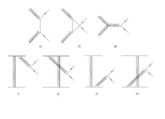
Figure 1: Feynman diagrams for the $pp\rightarrow Q\bar{Q}X$ process.

We used Sudakov decopmosition for the momenta of heavy quarks and the initial gluons: $p_{i}=\alpha_{i}P_{1}+\beta_{i}P_{2}+p_{i\perp},\,\,\,k_{1}=\alpha P_{1}+k_{1\perp},\,\,\,k_{2}=\beta P_{2}+k_{2\perp}$, $p_{1}^{2}=p_{2}^{2}=M^{2},\,\,\,k_{1}^{2}=k_{1T}^{2},\,\,\,k_{2}^{2}=k_{2T}^{2}$, where in the center of mass frame of colliding particles

$P_{1}=(E,0,0,E),\,\,\,P_{2}=(E,0,0,-E),\,\,\,E=\sqrt{s}/2,\,\,\,P_{1}^{2}=P_{2}^{2}=0,\,\,\,(P_{1}P_{2})=s/2$.

Sudakov variables are

$$\alpha_{1}=\frac{M_{1T}}{\sqrt{s}}\exp(y_{1}^{\ast}),\,\,\,\alpha_{2}=\frac{M_{2T}}{\sqrt{s}}\exp(y_{2}^{\ast}),\,\,\,\beta_{1}=\frac{M_{1T}}{\sqrt{s}}\exp(-y_{1}^{\ast}),\,\,\,\beta_{2}=\frac{M_{2T}}{\sqrt{s}}\exp(-y_{2}^{\ast}),$$

$k_{1T}+k_{2T}=p_{1T}+p_{2T},\,\,\,\alpha=\alpha_{1}+\alpha_{2},\,\,\,\beta=\beta_{1}+\beta_{2}$.

To guarantee gauge invariance, the process with off-shell incoming particles has to be embedded into the scaterring of on-shell particles. The second row of Fig. 1 includes non-factorizing diagrams which are factorized only in the sum. To make this factorization one can sum up these diagrams with the last diagram in the first row leading to one diagram with an effective Lipatov vertex by working in Feynman gauge [24]:

$$\Gamma^{\nu}(k_{1},k_{2})=\frac{2P_{1}P_{2}}{s}\left(\frac{2t_{1}+M^{2}_{T}}{\beta s}P_{1}^{\nu}-\frac{2t_{2}+M^{2}_{T}}{\alpha s}P_{2}^{\nu}-(k_{1T}-k_{2T})^{\nu}\right),$$ (12)

where $t_{1}=k_{1}^{2}=-{\mathbf{k}}_{1T}^{2},\,\,\,t_{2}=k_{2}^{2}=-{\mathbf{k}}_{2T}^{2},\,\,\,M_{T}^{2}=\hat{s}+({\mathbf{k}}_{1T}^{2}+{\mathbf{k}}_{2T}^{2})$.
This vertex obeys the Ward identity: $\Gamma^{\mu}(k_{1},k_{2})k_{1\mu}=0$. Then the last five diagrams in Fig. 1 are replaced by one diagram (Fig. 2).

Figure 2: Feynman diagrams explaining Lipatov vertex.

By neglecting the exchanged momentum in the coupling of gluons to incoming particles, we get an eikonal vertex which does not depend on the spin of the particle:

$${\bar{u}}(\lambda_{1}^{\prime},P_{1}-k_{1})\gamma^{\mu}u(\lambda_{1},P_{1})\,\,\,\,\,\to 2P_{1}^{\mu}\delta_{\lambda_{1}^{\prime},\lambda_{1}}.$$ (13)

Then it is possible to remove the external particle lines and attach so-called ”non-sense” polarization to the incoming gluons:

$$\epsilon_{k_{1}}^{\mu}={\sqrt{2}}P_{1}^{\mu}/{\sqrt{s}},\,\,\epsilon_{k_{2}}^{\mu}={\sqrt{2}}P_{2}^{\mu}/{\sqrt{s}}.$$ (14)

Instead of Feynman gauge, one can choose an appropriate axial gauge $n\bullet A=0$  ($n^{\mu}=aP_{1}^{\mu}+bP_{2}^{\mu}$).
The contraction of the eikonal coupling with the gluon polarization in this gauge

$$d_{\mu\nu}^{(n)}(k)=-g_{\mu\nu}+\frac{n_{\mu}k_{\nu}+k_{\mu}n_{\nu}}{nk}-n^{2}\frac{k_{\mu}k_{\nu}}{(nk)^{2}}$$ (15)

then reads

$$P_{1}^{\mu}d_{\mu\nu}^{(n)}(k_{1})=k_{1T\nu}/\alpha,\,\,\ P_{2}^{\mu}d_{\mu\nu}^{(n)}(k_{2})=k_{2T\nu}/\beta.$$ (16)

In such a physical gauge the non-factortizing diagrammes vanish since the direct connection of two eikonal couplings gives $P_{1}^{\mu}d_{\mu\nu}^{(n)}P_{2}^{\nu}=0$. It means the Lipatov vertex is to be replaced by the usual three gluon vertex. Then we can use the following matrix elements according to the diagrams in Fig. 1:

$$M_{1}=\bar{u}(p_{1})(-ig\gamma^{\mu})\varepsilon_{\mu}(k_{1})i{\hat{p}_{1}-\hat{k}_{1}+M\over(p_{1}-k_{1})^{2}-M^{2}}(-ig\gamma^{\nu})\varepsilon_{\nu}(k_{2})v(p_{2}),$$ (17)

$$M_{2}=\bar{u}(p_{1})(-ig\gamma^{\nu})\varepsilon_{\nu}(k_{2})i{\hat{p}_{1}-\hat{k}_{2}+M\over(p_{1}-k_{2})^{2}-M^{2}}(-ig\gamma^{\mu})\varepsilon_{\mu}(k_{1})v(p_{2}),$$ (18)

$$M_{3}=\bar{u}(p_{1})C^{\mu\nu\lambda}(-k_{1},-k_{2},k_{1}+k_{2})\,{g^{2}\varepsilon_{\mu}(k_{1})\varepsilon_{\nu}(k_{2})\over(k_{1}+k_{2})^{2}}\gamma_{\lambda}\,v(p_{2}),$$ (19)

where

$$C^{\mu\nu\lambda}(k_{1},k_{2},k_{3})=i((k_{2}-k_{1})^{\lambda}g^{\mu\nu}+(k_{3}-k_{2})^{\mu}g^{\nu\lambda}+(k_{1}-k_{3})^{\nu}g^{\lambda\mu})$$ (20)

is the standard three gluon vertex.

6 Numerical results

Recently we have demonstrated reasonable agreement between the $k_{T}$-factorization predictions and the Tevatron data on the $b$-quarks, $b\bar{b}$ di-jets, $B^{+}$- and $D$-mesons  [25]. Based on these results, here we give here analysis of the CMS [26, 27, 28] and LHCb [29] data in the framework of the $k_{T}$-factorization approach. We produced the relevant numerical calculations in two ways:

• We performed analytical parton-level calculations (which are labeled as LZ).

• The measured cross sections of heavy quark production was compared also with the predictions of full hadron level Monte Carlo event generator CASCADE.

In our numerical calculations we have used three different sets, namely the CCFM A0 (B0) and the KMR ones. The difference between A0 and B0 sets is connected with the different values of soft cut and width of the intrinsic ${\mathbf{k}}_{T}$ distribution. A reasonable description of the $F_{2}$ data can be achieved by both these sets. For the input, we have used the standard MSTW’2008 (LO) [30] (in LZ calculations) and the MRST 99 [31] (in CASCADE) sets. The unintegrated gluon distributions depend on the renormalization and factorization scales $\mu_{R}$ and $\mu_{F}$. We set $\mu_{R}^{2}=m_{Q}^{2}+({\mathbf{p}}_{1T}^{2}+{\mathbf{p}}_{2T}^{2})/2$, $\mu_{F}^{2}=\hat{s}+{\mathbf{Q}}_{T}^{2}$, where ${\mathbf{Q}}_{T}$ is the transverse momentum of the initial off-shell gluon pair, $m_{c}=1.4\pm 0.1$ GeV, $m_{b}=4.75\pm 0.25$ GeV. We use the LO formula for the coupling $\alpha_{s}(\mu_{R}^{2})$ with $n_{f}=4$ active quark flavors at $\Lambda_{\rm QCD}=200$ MeV, such that $\alpha_{s}(M_{Z}^{2})=0.1232$.

We begin the discussion by presenting our results for the muons originating from the semileptonic decays of the $b$ quarks. The CMS collaboration has measured the transverse momentum and the pseudorapidity distributions of muons from $b$-decays. The measurements have been performed in the kinematic range $p_{T}^{\mu}>6$ GeV and $|\eta^{\mu}|<2.1$ at the total center-of-mass energy $\sqrt{s}=7$ TeV.
To produce muons from $b$-quarks, we first convert $b$-quarks into $B$-mesons using the Peterson fragmentation function with default value $\epsilon_{b}=0.006$ and then simulate their semileptonic decay according to the standard electroweak theory taking into account the decays $b\to\mu$ as well as the cascade decay $b\to c\to\mu$.

The results of our calcilations are shown in Figs. 3 – 8 in the comparison with the LHC data (see [18] for more details). We obtain a good description of the data when using the CCFM-evolved (namely, A0) gluon distribution in LZ calculations. The shape and absolute normalization of measured $b$-flavored hadron cross sections at forward rapidities are reproduced well (see Fig. 6). The KMR and CCFM B0 predictions are somewhat below the data. In contrast with $b$ hadron and decay muon cross sections, the results for inclusive $b$-jet production based on the CCFM and KMR gluons are very similar to each other anda reasonable description of the data is obtained by all unintegrated gluon distributions under consideration.

The CASCADE predictions tend to lie slightly below the LZ ones and are rather close to the MC@NLO calculations (not shown). The observed difference between the LZ and CASCADE connects with the missing parton shower effects in the LZ evaluations. We have checked additionaly that the LZ and CASCADE predictions coincide at parton level..

Figs. 5 and 8 show the role of fragmentation and off-shelness effects in our calculations.

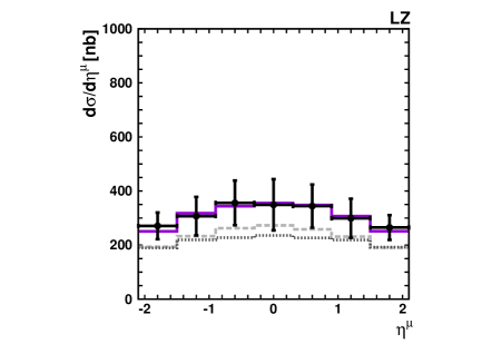
Figure 3: The pseudo-rapidity distributions of muons arising from the semileptonic decays of beauty quarks. The first column shows the LZ numerical results while the second one depicts the CASCADE predictions. The solid, dashed and dash-dotted, dotted histograms correspond to the results obtained with the CCFM A0, B0 and KMR unintegrated gluon densities. The experimental data are from CMS [26].

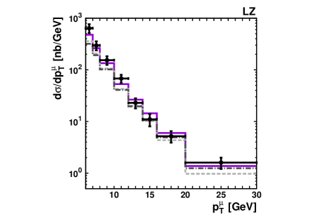
Figure 4: The transverse momentum distributions of muons arising from the semileptonic decays of beauty quarks. The first column shows the LZ numerical results while the second one depicts the CASCADE predictions. Notation of all histograms is the same as on previous slide. The experimental data are from CMS [26].

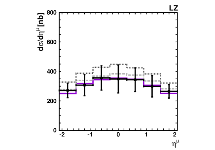
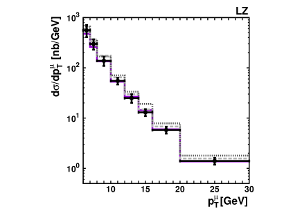
Figure 5: The dependence of our predictions on the fragmentation scheme. The solid, dashed and dash-dotted histograms correspond to the results obtained using the Peterson fragmentation function with $\epsilon_{b}=0.006,\epsilon_{b}=0.003$ and the non-perturbative fragmentation functions respectively. We use CCFM (A0) gluon density for illustration. The experimental data are from CMS [26].

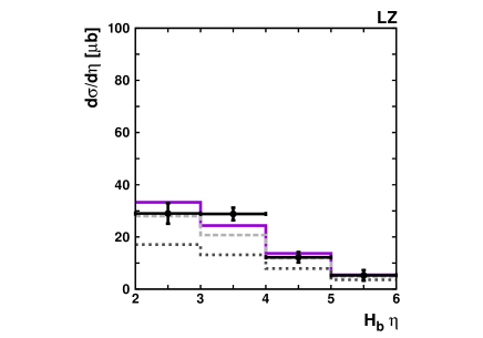
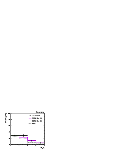
Figure 6: The pseudorapidity distributions of $b$-flavored hadrons at LHC. LZ results with the CCFM AO, BO and KMR uPDF. The experimental data are from LHCb [29].

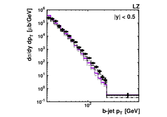
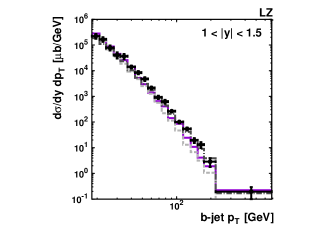
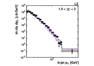
Figure 7: The differential cross sections $d\sigma/dy\,dp_{T}$ of inclusive $b$-jet production integrated over the specified $y$ intervals. The experimental data are from CMS [28]

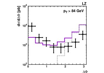
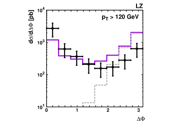
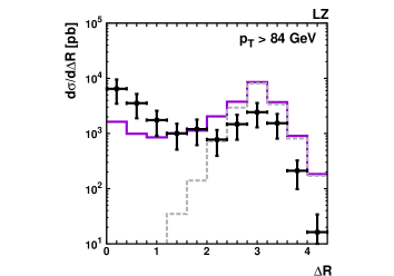
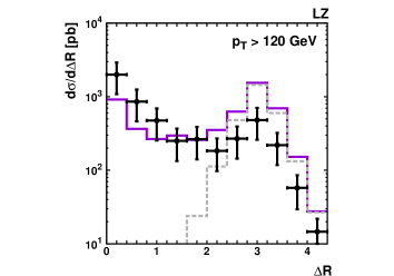
Figure 8: Importance of non-zero ${\mathbf{k}}_{T}$ of incoming gluons. Dotted histograms - the results obtained without the virtualities gluons and with ${\mathbf{k}}_{T}^{2}<\mu^{2}_{R}$ in matrix element. The CMS data [27].

7 Quarkonium production in the $k_{T}-$factorization approach

The production of prompt $J/\psi$($\Upsilon$)-mesons in $pp$-collisions can proceed via either direct gluon-gluon fusion or the production of $P$-wave states $\chi_{c}(\chi_{b}$) and $S$-wave state $\psi^{\prime}$ followed by their radiative decays $\chi_{c}(\chi_{b})\to J/\psi(\Upsilon)+\gamma$. In the $k_{T}-$factorization approach the direct mechanism corresponds to the partonic subprocess $g^{*}+g^{*}\to J/\psi(\Upsilon)+g$. The production of $P$-wave mesons is given by $g^{*}+g^{*}\to\chi_{c}(\chi_{b})$, and there is no emittion of any additional gluons. The feed-down contribution from $S$-wave state $\psi^{\prime}$ is described by $g^{*}+g^{*}\to\psi^{\prime}+g$.
The cross sections charmonium states depend on the renormalization and factorization scales $\mu_{R}$ and $\mu_{F}$. We set $\mu_{R}^{2}=m^{2}+{\mathbf{p}}_{T}^{2}$ and $\mu_{F}^{2}=\hat{s}+{\mathbf{Q}}_{T}^{2}$, where ${\mathbf{Q}}_{T}^{2}$ is the transverse momentum of initial off-shell gluon pair. Following to PDG [32], we set $m_{J/\psi}=3.097$ GeV, $m_{\chi c1}=3.511$ GeV, $m_{\chi c2}=3.556$ GeV, $m_{\psi^{\prime}}=3.686$ GeV and use the LO formula for the coupling constant $\alpha_{s}(\mu^{2})$ with $n_{f}=4$ quark flavours at $\Lambda_{QCD}=200$ Mev, such that $\alpha(M^{2}_{Z})=0.1232$.
The charmonium wave functions are taken to be equal to $|{\cal}R_{J/\psi}(0)|^{2}/4{\pi}=0.0876$ GeV³, $|{\cal}{R^{\prime}}_{\chi}(0)|^{2}=0.075$ GeV⁵, $|{\cal}R_{\psi^{\prime}}(0)|^{2}/4{\pi}=0.0391$ GeV³ and the following branching fractions are used $B(\chi_{c1}\to J/\psi+\gamma)=0.356,B(\chi_{c2}\to J/\psi+\gamma)=0.202,B(\psi^{\prime}\to J/\psi+X)=0.561$ and $B(J/\psi\to\mu^{+}\mu^{-})=0.0593$. Since the branching fraction for $\chi_{c0}\to J/\psi+\gamma$ decay is more than an order of magnitide smaller than for $\chi_{c1}$ and $\chi_{c2}$, we neglect its contribution to $J/\psi$ production. As $\psi^{\prime}\to J/\psi+X$ decay matrix elements are unknown, these events were generated according to the phase space.

Comparison the results of our calculations with the CMS [33], ATLAS [34] and LHCb [35] data are shown in Figs. 9 - 11 [19]. We see that the taking into account sole direct production is not sufficient to descibe the LHC data.We have obtained a good overall agreement between our predictions and the data when summing up the direct and feed-down contributions. The dependence of our numerical results on the uPDF is rather weak and the CCFM and KMR predictions are practically coincide. The difference between them can be observed at small $p_{T}$ or at large rapidities probed at the LHCb measerements. We have evaluated the polarizations parameters of prompt $J/\psi$ mesons in the kinematical region of CMS, ATLAS and LHCb measurements in the Collins-Soper and helicity frames (see [19]). We have took into account the contributions from the direcct and feed-dowm mechanisms. The qualitative predictions for the $J/\psi$ meson polarization are stable with respect to variations in the model parameters. Therefore future price measurements of the polarizations parameters of the $J/\psi$ mesons at the LHC will play crucial role in discriminating the different theoretical approaches.

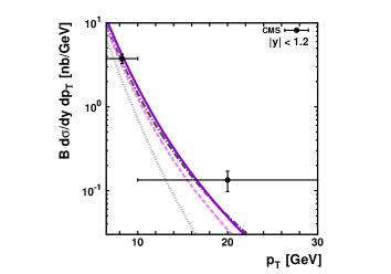
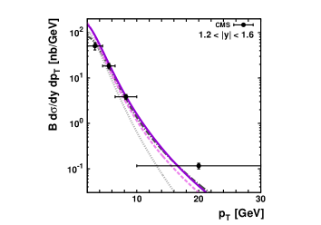
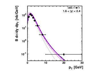
Figure 9: The differential cross sections $d\sigma/dydp_{T}$ of prompt $J/\psi$ production at LHC integrated over the specified $y$ intervals. Solid, dashed and dashed-dotted curves correspond to the results obtained using the CCFM A0, B0 and KMR uPDF. Dotted curves represent the contribution from sole direct production mechanism cal culated with the CCFM A0 uPDF. The CMS data [33].

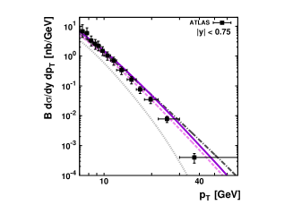
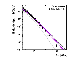
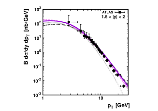
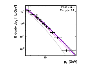
Figure 10: The differential cross sections $d\sigma/dydp_{T}$ of the $J/\psi$ production at LHC integrated over the specified $y$ intervals in comparison with the ATLAS data [34].

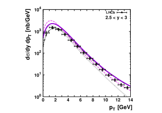
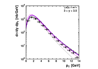
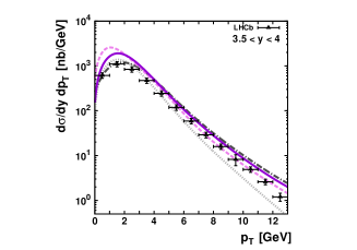
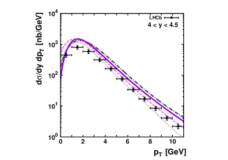
Figure 11: The differential cross sections $d\sigma/dydp_{T}$ of the $J/\psi$ production at LHC integrated over the specified $y$ inrervals in comparison with the LHCb data [35].

8 Conclusions

In the present time there is steady progress toward a better understanding of the $k_{T}$-factorization (high energy factorization) and the uPDF (TMD).
We have described the first exp. data of $b$-quark and $J/\psi$ production at LHC in the $k_{T}$-factorization approach. We have obtained reasonable agreement of our calculations and the first experimental data taken by the CMS and ATLAS Collaborations.
The dependence of our predictions on the uPDF appears at small transverse momenta and at large rapidities in $H_{b}$ and $J/\psi$ production covered by the LHCb experiment.
Our study has demonstrated also that in the framework of the $k_{T}$-factorization approach there is no need in a color octet contributions for the charmonium production at the LHC.
As it was shown in [19] the future experimental analyses of quarkonium polarization at LHC are very important and informative for discriminating the different theoretical models.

References

-
[1]
E.A. Kuraev, L.N. Lipatov and V.S. Fadin, Sov. Phys. JETP 44, 443 (1976);
E.A. Kuraev, L.N. Lipatov and V.S. Fadin, Sov. Phys. JETP 45, 199 (1977);
I.I. Balitsky and L.N. Lipatov, Sov. J. Nucl. Phys. 28, 822 (1978). - [2] L.V. Gribov, E.M. Levin, and M.G. Ryskin, Phys. Rep. 100, 1 (1983).
-
[3]
E.M. Levin, M.G. Ryskin, Yu.M. Shabelsky and A.G. Shuvaev, Sov. J. Nucl. Phys. 53, 657 (1991);
S. Catani, M. Ciafoloni and F. Hautmann, Nucl. Phys. B 366, 135 (1991);
J.C. Collins and R.K. Ellis, Nucl. Phys. B 360, 3 (1991). -
[4]
M. Ciafaloni, Nucl. Phys. B 296, 49 (1988);
S. Catani, F. Fiorani and G. Marchesini, Phys. Lett. B 234, 339 (1990);
S. Catani, F. Fiorani and G. Marchesini, Nucl. Phys. B 336, 18 (1990);
G. Marchesini, Nucl. Phys. B 445, 49 (1995). -
[5]
A.H. Mueller and J. Qiu, Nuscl. Phys. B 268, 427 (1986);
K. Golec-Biernat and M. Wusthoff, Phys. Rev D 59, 014017 (1999); D 60, 114023 (1999). -
[6]
I.I. Balitsky, Nucl. Phys. B 463, 99 (1996);
Y.V. Kovchegov, Phys. Rev. D 60, 034008 (1999). -
[7]
M. Gyulassy and L. McLerran, Nucl. Phys. A 750, 30 (2005);
A.V. Leonidov, Uspekhi Fiz. Nauk 175, 345 (2005). -
[8]
E. Iancu, Nucl. Phys. Proc. Suppl. 191, 281 (2009), arXiv:0901.0986 [hep-ph];
J.P. Blaizot, Nucl. Phys. A 854, 237 (2011). -
[9]
B. Andersson et al. (Small-x Collaboration), Eur. Phys. J. C 25, 77 (2002);
J. Andersen et al. (Small-x Collaboration) Eur. Phys. J. C 35, 67 (2004);
J. Andersen et al. (Small-x Collaboration) Eur. Phys. J. C 48, 53 (2006). -
[10]
F. Dominguez et al., Phys. Rev. D
83, 105005 (2011);
S.M. Aybat, T.C. Rogers, Phys. Rev. D 83, 114042 (2011);
I.O. Cherednikov, arXiv:1102.0892 [hep-ph]; I.O. Cherednikov and N.G. Stefanis, Int. J. Mod. Phys. Conf. Ser.4, 135 (2011), arXiv:1108.0811 [hep-ph]. - [11] http://www.pv.infn.it/ bacchett/TMDprogram.htm.
- [12] J.C. Collins, Foundations of Perturbati ve QCD (Cambridge University Press, Cambridge, 2011).
-
[13]
V. Barone, M. Genovese, N.N. Nikolaev, E. Predazzi and B.G. Zakharov, Phys. Lett. B 326, 161 (1994);
A. Bialas, H. Navelet and R. Peschanski, Nucl. Phys. B 593, 438 (2001). - [14] E. Avsar, arXiv:1108.1181 [hep-ph].
- [15] S. Marzani, Nucl. Phys. Proc. Suppl. 205 - 206, 25 (2010), arXiv:1006.2314 [hep-ph].
- [16] R.D. Ball and R.K. Ellis, JHEP 0105, 053 (2001).
- [17] R.D. Ball, Nucl. Phys. B 796, 137 (2008).
- [18] H. Jung, M. Krämer, A.V. Lipatov and N.P. Zotov, DESY 11-180, arXiv:1111.1942 [hep-ph].
- [19] S.P. Baranov, A.V. Lipatov and N. P. Zotov, DESY 11-143, arXiv:1108.2856 [hep-ph].
- [20] A.V. Lipatov, M.A. Malyshev and N.P. Zotov, this Proccedings.
- [21] M.A. Kimber, A.D Martin and M.G. Ryskin, Phys. Rev. D 63, 114027 (2001).
- [22] G. Watt, A.D. Martin and M.G. Ryskin, Eur. Phys. J. C 31, 73 (2003).
-
[23]
H. Jung, Comp. Phys. Comm. 143, 100 (2002);
H. Jung and G. Salam, Eur. Phys. J. C 19, 359 (2001);
H. Jung, S.P. Baranov, M. Deak et al., Eur. Phys. J. C 70, 1237 (2010). - [24] L.N. Lipatov, Sov. J. Nucl. Phys. 23, 338 (1976).
- [25] H. Jung, M. Krämer, A.V. Lipatov and N.P. Zotov, JHEP 1101, 085 (2011).
- [26] CMS Collaboration, JHEP 1103, 090 (2011).
- [27] CMS Collaboration, JHEP 1103, 136 (2011).
- [28] V. Chiochia, Nucl. Phys. A 855, 436 (2011).
- [29] LHCb Collaboration, Phys. Lett. B 694, 209 (2010).
- [30] A.D. Martin, W.J. Stirling, R.S. Thorne and G. Watt, Eur. Phys. J. C 63, 189 (2009).
- [31] A.D. Martin, R.G. Roberts, W.J. Stirling and R.S. Thorne, Eur. Phys. J. C 14, 133 (2000).
- [32] C. Amsler et al. (PDG Collaboration), Phys. Lett. B 667, 1 (2008).
- [33] CMS Collaboration, Eur. Phys. J. C 71, 1575 (2011).
- [34] G. Aad et al. (ATLAS Collaboration), Nucl. Phys. B 850, 387 (2011).
- [35] R. Aaij et al. (LHCb Collaboration), Eur. Phys. J. C 71, 1645 (2011).