A bottleneck model for bidirectional transport controlled by fluctuations

Abstract

We introduce a new model to study the oscillations of opposite flows sharing a common bottleneck and moving on two Totally Asymmetric Simple Exclusion Process (TASEP) lanes. We provide a theoretical analysis of the phase diagram, valid when the flow in the bottleneck is dominated by local stationary states. In particular, we predict and find an inhomogeneous high density phase, with a striped spatio-temporal structure. At the same time, our results also show that some other features of the model cannot be explained by the stationarity hypothesis and require consideration of the transients in the bottleneck at each reversal of the flow. In particular, we show that for short bottlenecks, the capacity of the system is at least as high as for uni-directional flow, in spite of having to empty the bottleneck at each reversal - a feature that can be explained only by efficient transients. Looking at more sensitive quantities like the distribution of flipping times, we show that, in most regimes, the bottleneck is driven by rare fluctuations and descriptions beyond the stationary state are required.

The understanding of the macroscopic behavior of complex systems out of equilibrium is one of the main challenges in modern statistical mechanics. A common feature of many non-equilibrium systems is the presence of a current in their stationary state, in contrast to equilibrium. A general framework describing these systems is still lacking, though the importance of current large deviations and their link with fluctuations theorems has been emphasized [1].

The absence of such general framework motivated the study of many oversimplified microscopical models, among which exclusion processes have been reference systems because they allow for extremely precise numerical results and exact analytical solutions in some cases. Exclusion processes are simple models defined on a discrete –usually one-dimensional– lattice, on which particles hop from site to site. Their role as a reference system is of particular importance for exact calculations of large deviations, the non-equilibrium counterpart of the free energy [2, 3]. At the same time, exclusion processes are a flexible tool to model various physical systems. Indeed, they capture the correct collective behavior of systems with very different length scales from social individuals, such as pedestrians [4], vehicles [5], ants [6, 4], to molecular systems as molecular motors [4, 3], and microscopical ones as quantum dots [7]. Furthermore exclusion processes are closely related [8] to growth phenomena described by the celebrated Kardar- Parisi-Zhang equation [9], and the universality of these phenomena has been confirmed in recent experiments in liquid crystals [10].

For the asymmetric simple exclusion process (ASEP) the full current probability distribution has been calculated for different boundary conditions [11, 12]. However, while the ASEP captures the proper behavior of particles moving on a single lane, it is obviously not appropriate to describe situations in which the particles (such as individuals or cars) move in few intersecting lanes. To describe such systems several one-dimensional exclusion processes must be coupled and the task of determining the current distributions becomes harder. Models for interacting parallel lanes (to describe e.g. the traffic on highways) have been introduced and studied [13]. In particular, in the so-called bridge models, two lanes share a finite number of sites (the ‘bridge’) [14]. Such systems have attracted a large interest due to the symmetry breaking that occurs in most cases [14, 15].

In this letter, we introduce a new model which couples two totally asymmetric simple exclusion process (TASEP) lanes with oppositely directed flows sharing a common bottleneck (see Fig. 1). In contrast to the bridge models, exchange of oppositely moving particles is not possible inside the bottleneck, because we impose that only particles going in one direction can go through the bottleneck at a given time. Therefore, particles going in the opposite direction have to wait until the whole bottleneck is empty before being allowed to go through. Our model can be seen as a representation of opposite pedestrian flows crossing e.g. at a door. The model is also relevant for other systems such as multiphase flows, or bidirectional molecular traffic across nuclear pores [16].

Figure 1: Schematic representation of the model.

We study this model with a combination of analytical and numerical techniques. The property that makes this model qualitatively different from previous ones is that the condition for reversing the flow inside the bottleneck (i.e. for having an empty bottleneck) is a rare event as soon as the bottleneck exceeds a few sites. Indeed, the dynamics of this system is driven by rare fluctuations, and is non trivial. For example, there exists a regime in which stop and go waves invade the whole system. Also, a counterintuitive feature of the model is that it can sustain in the bottleneck a current higher than the maximal current of a single lane system of infinite size.

1 The model

We define now the model more precisely. Particles move on two parallel tracks, modeled as two TASEP lanes. Both lanes share the same bottleneck of length $N_{b}$. We call ‘+’ (resp. ‘-’) the particles moving from left to right (right to left), represented as red (blue) particles in Fig. 1. We consider explicitly only the lanes of incoming particles (of length $L$). Thus outgoing lanes are shadowed in Fig. 1. Random sequential update is considered. Particles enter the lane with rate $\alpha$, hop forward with rate $p$ if the next site is empty, and leave the bottleneck with rate $\beta$. A particle enters the bottleneck with rate $p_{0}$ only if (i) there is no particle of the other species inside the bottleneck and (ii) the first site of the bottleneck is empty. We assume $p=p_{0}=1$, leaving only $\alpha$ and $\beta$ as the model parameters, in addition to the bottleneck and lanes lengths $N_{b}$ and $L$.

2 Phase diagram

By using the stationary properties of the TASEP, we infer the phase diagram (given in Fig. 2) of the system with bottleneck from simple phenomenological arguments. In the following, currents refer in general to the current of one given species of particles (and not the total current).

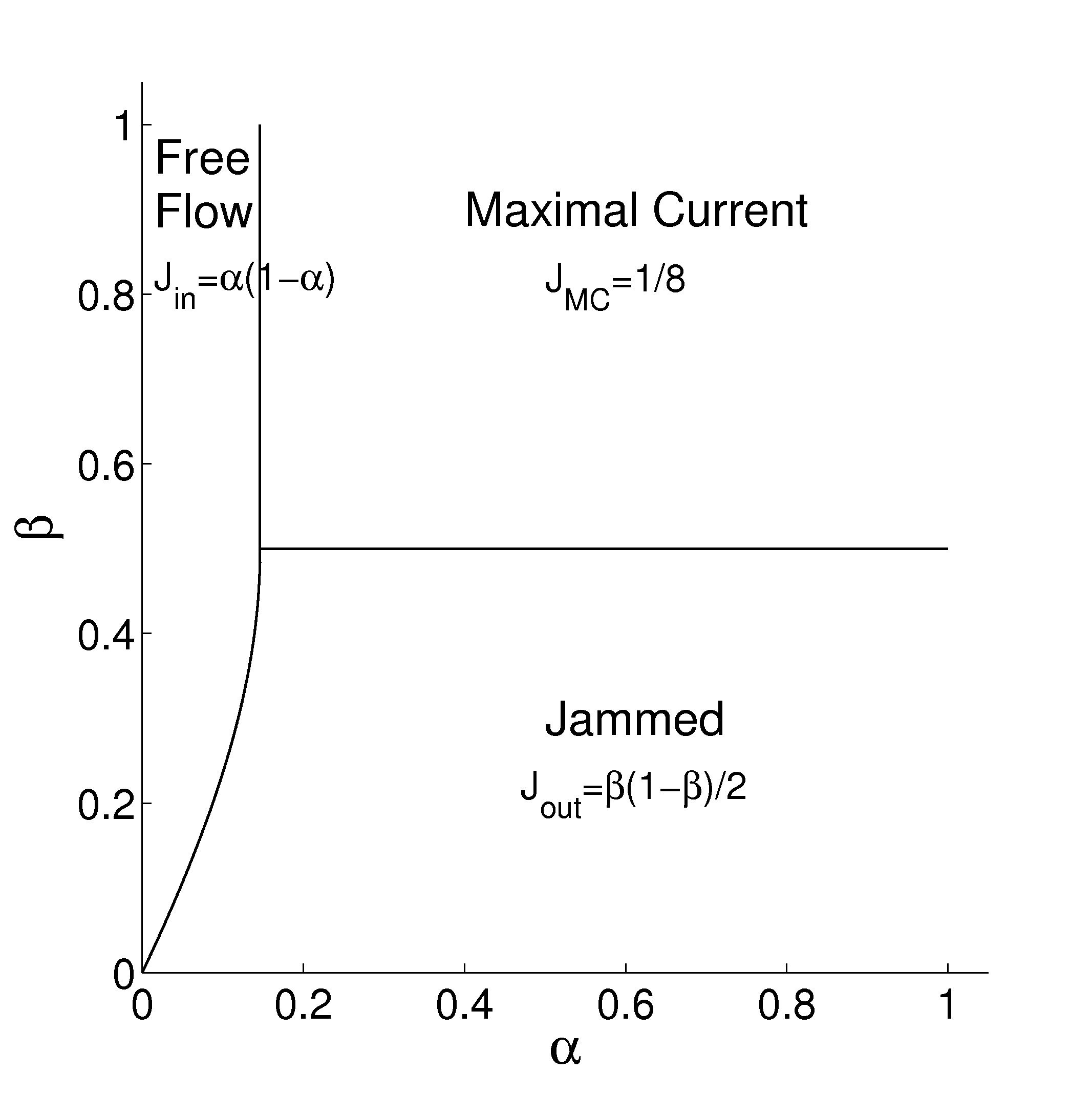
Figure 2: Phase diagram of the bottleneck model, predicted by the phenomenological approach.

For low $\alpha$ values, we expect a free flow (FF) phase driven by the entrance rate. For each species, the corresponding particle current and density are

$$J_{in}=\alpha(1-\alpha);\;\;\;\;\rho_{in}=\alpha.$$ (1)

For large $\alpha$ and small $\beta$, we expect an exit driven jammed (JJ) phase. When a species goes through the bottleneck for a long enough time, the system should become equivalent to a one-lane TASEP in stationary state, and the current should be $\beta(1-\beta)$. As the use of the bottleneck is shared between the two types of particles, each species can go through only half of the time. Neglecting the effects of the transients, on average the current is

$$J_{out}=\frac{1}{2}\beta(1-\beta).$$ (2)

We shall see that the particle distribution in incoming lanes is not homogeneous, and that, in contrast to current, density cannot be obtained from this mean field like approach.

The FF/JJ boundary is given by the solution of $J_{in}=J_{out}$, satisfying $\alpha_{c}(\beta)\to 0$ when $\beta\to 0$, i.e.

$$\alpha_{c}(\beta)=\frac{1}{2}-\frac{1}{2}\sqrt{1-2\beta(1-\beta)}.$$ (3)

The FF phase corresponds to $\alpha<\alpha_{c}(\beta)$.

When $\alpha>1/2$ and $\beta>1/2$, the single lane TASEP is in the maximal current (MC) phase, with a current equal to $1/4$. Again, if we neglect transients in the bottleneck, the average current must be half of this value:

$$J_{MC}=1/8.$$ (4)

The MC/FF boundary, obtained from $J_{in}=J_{MC}$, is given by $\alpha_{c}=(1-\sqrt{1/2})/2\simeq 0.146,$ while for the MC/JJ boundary, $J_{out}=J_{MC}$ provides $\beta_{c}=\frac{1}{2}.$

Figure 3: Average current as a function of $\alpha$, for different values of $\beta$. Symbols indicate numerical results obtained from Monte Carlo simulations for $L=50$ and $N_{b}=4$. The solid line gives the theoretical predictions for $\beta>1/2$, i.e. both for the free flow and the maximal current phase. Dashed lines give predictions for $\beta<1/2$ for the jammed phase with $\alpha>\alpha_{c}(\beta)$.

Monte Carlo simulations confirm these mean field predictions both for current and density in the FF phase [Eq. (1)], and for the current in the JJ phase [Eq. (2)] for values of $\beta$ not close to the MC boundary (see Fig. 3). By contrast, the current in the MC phase is systematically underestimated by this phenomenological approach. However, as seen in Fig. 4, the maximal current value (4) is recovered for long bottlenecks, for which a stationary state can be established in the bottleneck.

Figure 4: Average current against $\beta$ for different $N_{b}$, and $L=50$, $\alpha=0.6$. The dashed line gives the theoretical predictions for $\alpha=0.6$, both for the jammed and MC phase. For large bottlenecks the current saturates to $J_{MC}=1/8$.

For shorter bottlenecks, currents higher than the stationary maximal current $1/4$ can be obtained.

Interestingly, with our bi-directional model, we can even reach the capacity of a finite-size system of size $N_{b}$ [11] which would be fed by two incoming lanes, each transporting the maximal current and injecting particles on the same end of the bottleneck (in this case, flow would be unidirectional in the bottleneck and no flux reversal would be needed).

Hence the counterintuitive result according to which it is at least as efficient to have particles coming from both ends of the bottleneck than having all these particles coming from the same end. This high capacity can be obtained in spite of the fact that bidirectional traffic requires to empty the bottleneck at each flux reversal, a limitation which is compensated by very efficient transient states. Indeed, at each reversal of the current in the bottleneck, particles enter an empty system. Their motion is not hindered by predecessors, and thus high fluxes can be achieved.

3 Spatio-temporal structures

To characterize the dynamics of the system, we use a domain wall approach [17, 18] describing the system at a mesoscopic scale. We consider only the FF and JJ phases, since the domain wall approach is not appropriate to describe the MC phase (which has long-range correlations). In this approach, we neglect transients inside the bottleneck, and assume that currents and densities are given by stationary expressions.

First we describe the FF phase, and take the point of view of ‘+’ particles. When the bottleneck is closed, ‘+’ particles accumulate in front of the bottleneck, forming a queue of density $1$. The upstream end of the queue can be seen as a discontinuity (or a wall) separating the queue from the bulk. A new wall is created when the bottleneck opens. The queuing particles feed the bottleneck with a high effective injection rate, and a high density domain is installed in the bottleneck. Ignoring transients, this jammed domain imposed by the exit has density $1-\beta$ and current $\beta(1-\beta)$. Due to mass conservation, the wall between the jammed domain and the queue moves backwards with velocity $1-\beta$ until the whole queue is dissolved. Then, at the separation between the bulk FF phase and the jammed domain localized at the exit, a new wall forms and moves forward with velocity $V=\frac{\left[\beta(1-\beta)-\alpha(1-\alpha)\right]}{(1-\alpha-\beta)}.$ In order to understand which phase invades the bulk, we have to determine whether the FF domain will reach the entrance of the bottleneck before it closes again. This is the case if

$$\alpha(1-\alpha)\leq\frac{1}{2}\beta(1-\beta),$$ (5)

and assuming that the bottleneck is open and closed for the same period of time $\tau$ (which is true on average). Then the queue and the jammed domain stay localized near the bottleneck, and the bulk FF phase can be sustained. If condition (5) is not fulfilled, the bulk FF phase is slowly invaded by the queue, and cannot survive over long times. Note that Eq. (5) is indeed identical to condition (3) for the FF/JJ boundary.

Figure 5: Spatio-temporal plot in the jammed phase ($\alpha=0.6$, $\beta=0.2$, $L=100$, $N_{b}=2$). Both incoming TASEP lanes are shown, with the bottleneck in the middle. Particles (empty sites) are represented as black (white) spots.

Now we apply the same coarse-grained approach to the JJ phase to show that a homogeneous bulk density is not possible. Indeed, $\rho_{bulk}$ should satisfy $\rho_{bulk}(1-\rho_{bulk})=J_{out}$. However, when the bottleneck is closed, a queue of density $1$ is formed. The wall between this queue and the bulk density moves backwards with velocity $\rho_{bulk}$. Instead, when the bottleneck is open, the wall separating the exit driven jammed domain and the queue moves backwards only with velocity $1-\beta$. Thus, it cannot catch up with the previous wall, and the queue can never be entirely dissolved. When the bottleneck closes again, a new queue of density $1$ is formed, whose rear end also moves with velocity $1-\beta$ inside the exit driven phase. Then, regions of queuing particles with density $1$ alternate with regions of density $1-\beta$ and current $\beta(1-\beta)$, resulting in an overall striped jammed phase. This is confirmed by spatio-temporal plot in Fig. 5 obtained from simulations. Averaging over the stripes gives an actual bulk density

$$\rho_{out}=1-\frac{\beta}{2},$$ (6)

also confirmed by the Monte Carlo simulations.

4 Distribution of the oscillation periods

Until now, we considered the average value of the oscillation period $\tau$, which is a fluctuating variable. To perform a quantitative analysis, we define $T$ as the time during which the bottleneck is occupied by at least one particle of the type under consideration. After $T$, bottleneck is empty and a particle of either the same or opposite type can enter. Thus $T$ is not identical to $\tau$ but strongly related to it. We now consider the probability distribution $P(T)$, shown in Fig. 6.

We focus on the jammed state, though a similar analysis could be done in the FF phase. If we assume as before that a stationary state is established in the bottleneck, then the probability for the bottleneck to be empty should be $P_{\emptyset}=\beta^{N_{b}}$ at each time step and, if we neglect correlations between successive time steps, the distribution $P(T)=(1-P_{\emptyset})^{T-1}P_{\emptyset}$ follows. For $N_{b}=1$, the stationary state is established very rapidly. For larger $N_{b}$, non negligible corrections are present because there is a non vanishing relaxation time $\theta$ towards stationarity. The accuracy of our prediction for $P(T)$ depends on the ratio between the typical times $T$ and the relaxation time $\theta$. The typical time $T$ is expected to increase more rapidly with the bottleneck size $N_{b}$ than the relaxation time $\theta$, making our prediction more accurate for large $N_{b}$. Indeed, in Fig. 7 we observe that the relative error between our prediction and simulation results decreases again for large bottlenecks.

Figure 6: Distribution $P(T)$ for $N_{b}=4$, $\alpha=0.6$, $\beta=0.2$ and $L=400$. The blue solid line is the whole distribution. The other curves are the contributions to $P(T)$ corresponding to the passage of at most $N_{max}$ particles through the bottleneck during the time interval $T$.

For all $N_{b}$, the prediction works better for small $\beta$, and the difference between theory and numerics increases when the MC phase is approached. Indeed, when $\beta$ increases, $P_{\emptyset}$ increases, and the typical $T$ value decreases. It can then become smaller than the relaxation time $\theta$ and a description of transients becomes necessary. Besides, the queues may not have enough time to form and thus do not overfeed the bottleneck.

Figure 7: Relative error between the numerical result and theoretical prediction for the decay rate of the tail of $P(T)$. Error is plotted against $N_{b}$, for various $\beta$, $L=100$ or $400$, $\alpha=0.6$. Lines are guides to the eyes.

Another feature visible in Fig. 6 is that there is an important contribution to $P(T)$ from events during which only a single or very few particles pass through the bottleneck. When these events occur, the system explores only very special configurations, which are not representative of the whole stationary distribution. Thus the system is still in a transient state when the next reversal occurs.

As a conclusion the dynamics for the reversal of the flux actually involves two quite different mechanisms (one based on stationarity and the other involving transients), and exhibits some kind of intermittency, with long periods of one-directional flows alternating with rapid switches. In order to have a full description of the dynamics of the flux reversal, not only the transient nature of the incoming flows in the bottleneck should be taken into account, but also the correlations between successive switches.

5 Conclusions

We have introduced a new model for bidirectional transport with a bottleneck. We have shown that theoretical considerations, based on the stationarity hypothesis for the flow inside the bottleneck, allow to predict with a good accuracy the phase diagram, and the values of the currents in the free flow phase, in the jammed phase, and in the MC phase for long bottlenecks. For short bottlenecks, transients dominate the behavior of the system, and as a consequence large values of the current can be observed, in spite of the cost of having to empty the bottleneck at each reversal of the flux. These transients could be studied by exploiting the exact results obtained for a single TASEP with a step initial condition [8, 20, 21].

The jammed phase turns out to have a striped structure. In spite of the similarity with [19], here the striped phase can be sustained in the bulk without any modification of the standard TASEP bulk rules. It should be noted that this striped phase results from a self-regulated dynamics for the flux reversal in the bottleneck. Though an assumption of constant reversal periods succeeds in predicting the striped phase density, we find that actually the structure of the distribution of the bottleneck occupation times $P(T)$ is more complex and emerges from two different mechanism. The tail of the distribution can be explained through our phenomenological approach assuming a 1-lane stationary state in the bottleneck. However, this prediction is valid only for small $\beta$, and in any case cannot explain the shape of the distribution around its maximum. A large part of the distribution is due to non-typical events where only a few particles go through the bottleneck. A complete understanding of $P(T)$ should involve the study of non-stationary distributions and correlations between flux reversals.

To conclude, the main feature that puts this new model apart from others in the literature is that fluctuations localized in the bottleneck can have a macroscopic effect on the whole system. It provides a sensitive test for different theoretical approaches and can be easily tested numerically. While a phenomenological approach assuming a stationary state in the bottleneck gives surprisingly good predictions for the free flow and part of the jammed phase, some other observations trigger much more complex questions involving non-stationary and correlated behaviors. While we concentrated on identical lanes without directional bias, one can, of course, consider asymmetries either in particles species or capacities of the lanes which are of interest for different applications.

- [1] J.L. Lebowitz and H. Spohn, J. Stat. Phys. 95, 333-365 (1999); D.J. Evans, E.G.D. Cohen, and G.P. Morriss, Phys. Rev. Lett. 71, 2401 (1993).
- [2] B. Derrida, J. Stat. Mech. P07023 (2007); B. Derrida, J. Stat. Mech. P01030 (2011).
- [3] T. Chou, K. Mallick, and R.K.P. Zia, Rep. Prog. Phys. 74, 116601 (2011).
- [4] D. Chowdhury, A. Schadschneider, and K. Nishinari, Phys. Life Rev. 2, 318 (2005);
- [5] D. Chowdhury, L. Santen, and A. Schadschneider, Phys. Rep. 329, 199 (2000).
- [6] A. John, A. Schadschneider, D. Chowdhury, and K. Nishinari, Phys. Rev. Lett. 102, 108001 (2009).
- [7] T. Karzig and F. von Oppen, Phys. Rev. B 81, 045317 (2010).
- [8] K. Johansson, Comm. Math. Phys. 209, 437 (2000); C.A. Tracy and H. Widom, Comm. Math. Phys. 290, 129 (2009); J. Math. Phys. 50, 095204 (2009); T. Sasamoto and H. Spohn, Phys. Rev. Lett. 104, 230602 (2010); P. Calabrese, P. Le Doussal, and A. Rosso, Eur. Phys. Lett. 90, 20002 (2010); V. Dotsenko, Eur. Phys. Lett. 90, 20003 (2010).
- [9] M. Kardar, G. Parisi, and Y.C. Zhang, Phys. Rev. Lett. 56, 889 (1986).
- [10] K.A. Takeuchi, M. Sano, T. Sasamoto, and H. Spohn, Sci. Rep. (Nature) 1, 34 (2011); K.A. Takeuchi and M. Sano, Phys. Rev. Lett. 104, 230601 (2010).
- [11] B. Derrida, M.R. Evans, V. Hakim, and V. Pasquier, J. Phys. A 26, 1493 (1993).
- [12] B. Derrida and J.L. Lebowitz, Phys. Rev. Lett. 80, 209 (1998); D.S. Lee and D. Kim, Phys. Rev. E 59, 6476 (1999); R.A. Blythe and M. R. Evans, J. Phys. A 40, R333 (2007); C. Appert-Rolland et. al., Phys. Rev. E 78, 021122 (2008); J. de Gier and F.H.L. Essler, Phys. Rev. Lett. 107, 010602 (2011).
- [13] T. Reichenbach, T. Franosch, and E. Frey, Phys. Rev. Lett. 97, 050603 (2006); C. Schiffmann, C. Appert-Rolland, and L. Santen, J. Stat. Mech. P06002 (2010); M.R. Evans, Y. Kafri, K.E.P. Sugden, and J. Tailleur, J. Stat. Mech. P06009 (2011).
- [14] M.R. Evans, D. P. Foster, C. Godrèche, and D. Mukamel, Phys. Rev. Lett. 74, 208 (1995).
- [15] V. Popkov, M.R. Evans, and D. Mukamel, J. Phys. A: Math. Theo. 41, 432002 (2008); D.W. Erickson, G. Pruessner, B. Schmittmann, and R.K.P. Zia, J. Phys. A: Math. Gen. 38, L659 (2005); S. Gupta, D. Mukamel, and G. Schütz, J. Phys. A - Math. Theo. 42, 485002 (2009); S. Großkinsky, G.M. Schütz, and R.D. Willmann, J. Stat. Phys. 128, 587 (2007).
- [16] R. Kapon, A. Topchik, D. Mukamel, and Z. Reich, Physical Biology 5, 036001 (2008).
- [17] A.B. Kolomeisky, G.M. Schütz, E.B. Kolomeisky, and J.P. Straley, J. Phys. A: Math. Gen. 31, 6911 (1998).
- [18] L. Santen and C. Appert, J. Stat. Phys. 106, 187 (2002).
- [19] C. Appert and L. Santen, Phys. Rev. Lett. 86, 2498 (2001).
- [20] B. Derrida and A. Gerschenfeld, J. Stat. Phys. 137, 978 (2009).
- [21] C.A. Tracy and H. Widom, J. Stat. Phys. 137, 825 (2009).