Vertex Nomination via Content and Context

Glen A. Coppersmith and Carey E. Priebe

Human Language Technology Center of Excellence

Johns Hopkins University

Abstract

If I know of a few persons of interest, how can a combination of human language technology and graph theory help me find other people similarly interesting? If I know of a few people committing a crime, how can I determine their co-conspirators? Given a set of actors deemed interesting, we seek other actors who are similarly interesting. We use a collection of communications encoded as an attributed graph, where vertices represent actors and edges connect pairs of actors that communicate. Attached to each edge is the set of documents wherein that pair of actors communicate, providing content in context – the communication topic in the context of who communicates with whom. In these documents, our identified interesting actors communicate amongst each other and with other actors whose interestingness is unknown. Our objective is to nominate the most likely interesting vertex from all vertices with unknown interestingness. As an illustrative example, the Enron email corpus consists of communications between actors, some of which are allegedly committing fraud. Some of their fraudulent activity is captured in emails, along with many innocuous emails (both between the fraudsters and between the other employees of Enron); we are given the identities of a few fraudster vertices and asked to nominate other vertices in the graph as likely representing other actors committing fraud. Foundational theory and initial experimental results indicate that approaching this task with a joint model of content and context improves the performance (as measured by standard information retrieval measures) over either content or context alone.

1 Introduction

Given a set of documents containing communications among a collection of actors and an identified subset of actors deemed interesting, we wish to select actors from outside the identified set who exhibit similar behavior to the identified interesting actors. For a concrete example, within the Enron email collection (see, e.g., Priebe et al., (2005)) is a set of executives and traders allegedly committing fraud. If we know the identities of a subset of the fraudsters, can we nominate other people from the company as likely fraudsters? We assume that what indicates that actors are interesting (fraudulent) is manifest both in the topics about which they communicate (the content of their messages) and with whom in the company they communicate (the context of their messages). We conceptualize this as an attributed graph, where each vertex is an actor and pairs of actors that communicate are connected by edges. The edges are attributed by the content of the messages exchanged (in our case, represented as a distribution over topics). We design and evaluate a family of test statistics that score each actor (vertex) based on the content and context of their email communications (edges). We nominate vertices from outside the identified set as likely to be interesting. This task has noted similarities to the Netflix challenge (e.g., Bell et al., (2008)), recommender systems (Resnick and Varian, (1997) and contents of the special issue), and detecting communities of interest (e.g. Cortes et al., (2002)).

Information useful for the vertex nomination task might be encoded in both content and context. It is reasonable to assume that test statistics based on either content alone or context alone would have some efficacy for vertex nomination, but statistics which take advantage of both content and context might provide superior inferential capability (e.g. Priebe et al., 2010b ). Selecting test statistics useful for this task (or selecting the uniformly most powerful test statistic against some specified composite alternative) is both interesting and decidedly nontrivial. (See Priebe et al., 2010a for a summary of inferential complexity in a related task in perhaps the simplest possible model – without content.) We set up a deceptively simple generative model (described in Section 2 and depicted in Figure 1) to study this task and present results from simulations and experiments on real data (the Enron email corpus).

The possible space of test statistics is practically limitless, even for this simple setting. For tractability, we limit ourselves to a simple family of linear fusion statistics (Section 3.1) and demonstrate how their performance for this task depends on many underlying factors (manifest as parameters in the generative model and latent qualities of the data). The optimal performance is found in a fusion of content and context rather than either alone, in both simulated and observed data (Sections 4 and 5 respectively).

This paper proceeds as follows: Section 2 spells out our assumptions and describes the joint model of content and context, Section 3 describes the experimental and evaluation methods used, Section 4 describes simulation experiments where the content and context is generated according to our model, Section 5 demonstrates that (A) our assumptions are reasonable (and real data corresponding to the assumptions does naturally occur), (B) when our assumptions are met, vertex nomination works, and (C) when our assumptions are met, the fusion of content and context is superior to either alone, and Section 6 makes concluding remarks and discusses future directions.

The appendix details our data set, the Enron email corpus.

2 Model

We base our model upon two assumptions, detailed below. Specifically, when the physical world exhibits a group of interest that meets these assumptions, our model is reasonable (as demonstrated in Section 5). We observe communications among our identified interesting set, among our candidate set, and between actors in the identified set and actors in the candidate set.

• Assumption 1: Pairs of vertices in the group of interest (identified and not identified) communicate among themselves with a different frequency than other pairs.

• Assumption 2: The group of interest communicates about topics in different proportions than the population of actors as a whole.

The context information available for vertex nomination is derived from Assumption 1, while the content information is derived from Assumption 2.

Let $G=(V,E,\phi_{V},\phi_{E})$ be the simplest of attributed graphs ($G$ is undirected, with no self-loops, no multi-edges and no hyper-edges). Let $V$ be the set of vertices (actors) and $E$ be the set of edges (communication between pairs of actors). Specifically, $E\subset V^{(2)}$, where $V^{(2)}$ denotes the set of unordered pairs of vertices. Attribution functions $\phi_{V}:V\to\Phi_{V}$ and $\phi_{E}:V^{(2)}\to\Phi_{E}$ place (categorical) attributes on the vertices and edges, respectively, where $\Phi_{V}=\{1,...,K_{V}\}$, $\Phi_{E}=\{0,1,...,K_{E}\}$ and $K_{V}$ is the number of vertex attributes (interesting and not interesting for our purposes) and $K_{E}$ is the number of edge attributes (topics for our purposes); $\phi_{E}=0$ represents a non-observed edge, so for all $e\notin E$, $\phi_{E}(e)=0$ and for all $e\in E$, $\phi_{E}(e)\in\{1,...,K_{E}\}$. For this investigation, $K_{V}=K_{E}=2$ and $\Phi_{V}=\Phi_{E}=\{red,green\}$. We use $red$ and $1$ interchangeably, as appropriate for the context. Likewise for $green$ and $2$.

For our investigation, we use a simple edge- and vertex-attributed independent edge model. We use a stochastic block-model random graph (sometimes referred to as a “kidney-egg” or $\kappa$ graph), where there is a “chatter” group present – a subset of the actors which communicate amongst themselves in excess of what is expected from the activity present in the rest of the graph and with a topic distribution different from that governing the rest of the graph. As depicted in Figure 1, $\kappa(n,p,m,s)$ is a random graph model Bollobás, (2001) on $n$ vertices ($|V|=n$); $|\{v:\phi_{V}(v)=1\}|=m$, so $m$ vertices have the attribute of interest ($red$) and communicate differently than the collection $\{v:\phi_{V}(v)=2\}$ of $n-m$ not of interest ($green$) vertices. The edge attribute for a pair of vertices $u,v$ with $\phi_{V}(u)=\phi_{V}(v)=1$ is governed by the probability vector $s=[s_{0},s_{1},s_{2}]^{\prime}$ where $s_{1}$ is the probability that the edge is $red$ ($\phi_{E}(uv)=1$), $s_{2}$ is the probability that the edge is $green$ ($\phi_{E}(uv)=2$), and $s_{0}$ is the probability of no edge; edge attributes for all other pairs of vertices are governed by $p=[p_{0},p_{1},p_{2}]^{\prime}$. Like $s$, $p_{1}$ is the probability of a $red$ edge, $p_{2}$ is the probability of a $green$ edge and $p_{0}$ is the probability of no edge.

The observed graph includes occlusion of most of the vertex attributes: $G{{}^{\prime}}=(V,E,\phi_{V},\phi{{}^{\prime}}_{V},\phi_{E})$ is a $\kappa(n,p,m,s;m^{\prime})$ graph where $\phi{{}^{\prime}}_{V}:V\to\Phi_{V}\cup\{0\}$ and $\phi_{V}(v)=0$ denotes that the attribute for vertex $v$ is occluded. For our particular setting, all observed attributes are $red$ and we observe no $green$ attributes (Figure 1). We let $\mathcal{M}=\{v:\phi_{V}(v)=1)\}$ be the set of vertices with true $red$ attributes. Our identified set – the set of vertices with observed (true) $red$ attributes – is given by $\mathcal{M}^{\prime}=\{v:\phi{{}^{\prime}}_{V}(v)=1\}$ and $|\mathcal{M}^{\prime}|=m^{\prime}$. (We assume that the identified set $\mathcal{M}^{\prime}\subset\mathcal{M}$ is selected at random.) The candidate set is $V\setminus\mathcal{M}^{\prime}$. We assume that there is no error in the vertex-attributes – just occlusion; in addition, we assume that we observe the attributes on all edges, and there is no error in the edge-attributes.

We assume that $n>>m>m^{\prime}>0$. That is, there is at least one vertex known to be of interest ($m^{\prime}\geq 1$), which allows the set of context measures we employ to measure functions of the graph-proximity to a member of $\mathcal{M}^{\prime}$. We also assume that candidate set $V\setminus\mathcal{M}^{\prime}$ contains at least one true $red$ ($m>m^{\prime}$) and at least one true $green$ ($n>m$) vertex. (The question of whether or not there exist any $red$ vertices in the candidate set is an interesting one; we do not directly address it here, but the methods described here do inform how one might approach that question.)

Figure 1: Our model, a $\kappa(n,p,m,s;m^{\prime})$ graph with $n=|V|$ vertices, $m=|\mathcal{M}|$ of which have attribute $red$ and $n-m=|V\setminus\mathcal{M}|$ of which have attribute $green$. We observe attributes for only $m^{\prime}=|\mathcal{M}^{\prime}|$ identified set vertices (filled circles) with the remaining $n-m^{\prime}=|V\setminus\mathcal{M}^{\prime}|$ candidate set vertices (open circles) having occluded attributes. Edges with attribute $green$ are of the topic not of interest ($2$) and $red$ edges are topic of interest ($1$). Pairs of $red$ vertices (regardless of occlusion) are connected according to probability distribution over topics $s$, while pairs of vertices where at least one is labeled $green$ are connected according to $p$. The vertex nomination task is to select one vertex from the candidate set $V\setminus\mathcal{M}^{\prime}$  (the vertices with occluded attributes, shown here as open circles) that is in $\mathcal{M}\setminus\mathcal{M}^{\prime}$  (truly $red$).

To rephrase the inference task in our freshly minted notation: We are given a graph $G^{\prime}$ on vertices $V$, $m$ of which have attribute $red$ ($\mathcal{M}\subset V$) and $n-m$ of which have attribute $green$ ($V\setminus\mathcal{M}$). All vertex-attributes are occluded save $m^{\prime}$ drawn from the set $\mathcal{M}$ ($\mathcal{M}^{\prime}\subset\mathcal{M}$); thus all observed vertex-attributes are $red$. We wish to rank order all vertices with occluded attributes – the candidate set $V\setminus\mathcal{M}^{\prime}$ – according to their similarity to the identified set $\mathcal{M}^{\prime}$. Performance is judged by how high in the ranked list of candidate vertices $V\setminus\mathcal{M}^{\prime}$ the vertices $\mathcal{M}\setminus\mathcal{M}^{\prime}$ with occluded (but truly $red$) attributes fall.

3 Methods

3.1 Statistics

We employ test statistics, based on the content and context of each vertex and its communications, to rank-order the candidate set $V\setminus\mathcal{M}^{\prime}$ for nomination. Consider a vertex $v$ in the candidate set $V\setminus\mathcal{M}^{\prime}$. If $p_{2}=s_{2}$ and $p_{1}<s_{1}$, then $v\in\mathcal{M}\setminus\mathcal{M}^{\prime}$ will have a stochastically larger value for both the number of known $red$ vertices adjacent to $v$ and the number of $red$ edges incident to $v$. This observation gives rise to the observation that the posterior probability of class membership $\rho(v)=P[\phi_{V}(v)=1|G^{\prime},\phi^{\prime}_{V}(v)=0]$ is monotonically increasing in both the context-only statistic

$$T^{0}(v)=\displaystyle\sum_{u\in\{w:wv\in E\}}\mathbb{I}\left\{\phi^{\prime}_{V}(u)=1\right\}$$ (1)

and the content-only statistic

$$T^{1}(v)=\displaystyle\sum_{uv\in E}\mathbb{I}\left\{\phi_{E}(uv)=1\right\}.$$ (2)

This in turn motivates the class of linear fusion statistics

$$T^{\gamma}(v)=(1-\gamma)T^{0}(v)+\gamma T^{1}(v).$$ (3)

Larger scores are more indicative of membership in $\mathcal{M}$. The parameter $\gamma$ determines the relative weight of content and context information. We rank each vertex $v$ in the candidate set $V\setminus\mathcal{M}^{\prime}$ for nomination as a likely member of $\mathcal{M}$ according to $T^{\gamma}(v)$. Let $\gamma^{\star}$ denote the fusion parameter which yields the highest performance.

For our independent edge model $\kappa(n,p,m,s;m^{\prime})$, the joint distribution of $T^{0}(v),T^{1}(v)$ is available: for $v\in V\setminus\mathcal{M}$, we have

$$T^{0}(v;G) \sim Bin(m^{\prime},p_{1}+p_{2}),$$

$$T^{1}(v;G) \sim Bin(n-1,p_{1}),$$

$$T^{1}|T^{0}=c \sim Bin(c,\frac{p_{1}}{p_{1}+p_{2}})+_{ind}Bin(n-1-m^{\prime},p_{1}),$$

while for $v\in\mathcal{M}\setminus\mathcal{M}^{\prime}$, we have

$$T^{0}(v;G) \sim Bin(m^{\prime},s_{1}+s_{2}),$$

$$T^{1}(v;G) \sim Bin(m-1,s_{1})+_{ind}Bin(n-m,p_{1}),$$

$$T^{1}|T^{0}=c \sim Bin(c,\frac{s_{1}}{s_{1}+s_{2}})+_{ind}Bin(m-1-m^{\prime},s_{1})$$

$$+_{ind}Bin(n-m,p_{1}).$$

For each candidate $v\in V\setminus\mathcal{M}^{\prime}$, we calculate $T^{\gamma}$, where $\gamma\in(0,1)$. For some plots we select a few illustrative values of $\gamma$, rather than plotting the entire range: $\gamma=0$ for context-only (represented on plots by “X”), $\gamma=1$ for content-only (represented on plots by “N”), $\gamma=0.5$ for (one particular instantiation of) fusion of content and context (represented on plots by “+”), and $\gamma=\gamma^{\star}$ for the linear fusion of content and context with the optimal performance (represented on plots by “*”).

For a given $\gamma$, we rank vertices for nomination according to $T^{\gamma}$ and consider the ordered candidates $v^{\gamma}_{(1)},v^{\gamma}_{(2)},\cdots,v^{\gamma}_{(n-m^{\prime})}$. E.g., considering vertices in the candidate set $V\setminus\mathcal{M}^{\prime}$, we have $v^{\gamma}_{(1)}=\arg\max_{v}T^{\gamma}(v)$, $v^{\gamma}_{(2)}$ is the vertex associated with the second largest value of $T^{\gamma}(v)$, etc. We evaluate the efficacy of each $T^{\gamma}$ according to three evaluation criteria, described below.

3.2 Evaluation Criteria

• Probability Correct

  If we nominate one vertex based on the values of the linear fusion statistic, then performance can be measured based on whether this nominee is in fact truly red – the success at rank 1 (S@1):

  $$\mbox{S@1}(\gamma)=\mathbb{I}\{v^{\gamma}_{(1)}\in\mathcal{M}\setminus\mathcal{M}^{\prime}\}.$$ (4)

  For a random experiment, we consider $E\left[\mbox{S@1}(\gamma)\right]$.

• Mean Reciprocal Rank

  Reciprocal rank (RR) is a measure of how far down a ranked list one must go to find the first truly red vertex:

  $$\mbox{RR}(\gamma)=\left(\min\{i:v^{\gamma}_{(i)}\in\mathcal{M}\setminus\mathcal{M}^{\prime}\}\right)^{-1}.$$ (5)

  For a random experiment, we consider the mean reciprocal rank

  $$\mbox{MRR}(\gamma)=E\left[\mbox{RR}(\gamma)\right].$$ (6)

• Mean Average Precision

  Average precision (AP) examines the placement within a ranked list of all truly red vertices – the average of the precision at the rank of each truly red vertex. We define precision at rank $r$ as

  $$Pre(r,\gamma)=\frac{\displaystyle\sum_{i=1}^{r}\mathbb{I}\{v^{\gamma}_{(i)}\in\mathcal{M}\setminus\mathcal{M}^{\prime}\}}{r}$$ (7)

  and average precision as

  $$\mbox{AP}(\gamma)=\frac{\displaystyle\sum_{i=1}^{|V\setminus\mathcal{M}^{\prime}|}\mathbb{I}\{v^{\gamma}_{(i)}\in\mathcal{M}\setminus\mathcal{M}^{\prime}\}Pre(i,\gamma)}{|\mathcal{M}\setminus\mathcal{M}^{\prime}|}.$$ (8)

  For a random experiment, we define the mean average precision

  $$\mbox{MAP}(\gamma)=E\left[\mbox{AP}(\gamma)\right].$$ (9)

Section 4 demonstrates that these measures are all highly correlated, as is further explored by Buckley and Voorhees, (2005). For our experiments, the relative ranking of vertex nomination methods is consistent across evaluation measures.

4 Simulation Experiments

We evaluate the performance of content and context fusion via simulation in the $\kappa(n,p,m,s;m^{\prime})$ model.

We consider $p,s$ in the standard 2-simplex $S^{2}=\{x\in\mathbb{R}^{3}:x_{i}\geq 0,\sum_{i}x_{i}=1\}$, constrained so that $s_{2}=p_{2}$ (so the probability of $green$ content being present is the same throughout the graph) and $s_{1}>p_{1}$ (so the probability of $red$ content being present is greater for edges that connect pairs in $\mathcal{M}$ than for all other pairs). (Note that this implies $s_{0}<p_{0}$, so also overall connectivity probability is greater for edges that connect pairs in $\mathcal{M}$ than for all other pairs.) We use $n=184$ (the number of actors in our Enron email corpus) and consider various values of $m,m^{\prime}$ such that $n>>m>m^{\prime}>0$. We assess performance using the three evaluation criteria, $E[\mbox{S@1}(\gamma)]$, $\mbox{MRR}(\gamma)$, and $\mbox{MAP}(\gamma)$, introduced in Section 3.2, for $\gamma\in[0,1]$.

Figure 2 presents performance using $\mbox{MAP}(\gamma)$ for

$$\kappa(n=184,p=[0.6,0.2,0.2]^{\prime},m,s=[0.4,0.4,0.2]^{\prime};m^{\prime}=m/4)$$

as we vary $m$. For small $m$, all our fusion statistics perform equally poorly. (The far leftmost point in Figure 2 represents $m=4$ and $m^{\prime}=1$, where almost no information is available.) As $m$ (and hence $m^{\prime}=m/4$) increases, fusion of content and context provides superior performance: $\gamma=0.5$ and $\gamma=\gamma^{\star}$ are superior to either $\gamma=1$ or $\gamma=0$ alone.

Figure 2: Context, content, arbitrary linear fusion, and optimal linear fusion ($\gamma=\{0,1,0.5,\gamma^{\star}\}$ respectively) results for $\mbox{MAP}(\gamma)$ in the $\kappa(n=184,p=[0.6,0.2,0.2]^{\prime},m,s=[0.4,0.4,0.2]^{\prime};m^{\prime}=m/4)$ model, as we vary $m$. We plot $m$ on the $x$-axis and $\mbox{MAP}(\gamma)$ on the $y$-axis. Content ($\gamma=1$) is represented by points labeled “N”, context $(\gamma=0)$ by points labeled “X”, arbitrary linear fusion ($\gamma=0.5$) by points labeled “+”, and optimal linear fusion ($\gamma=\gamma^{\star}$) by points labeled “*”. Results are obtained via $1000$ Monte Carlo replicates. The green dashed line denotes chance performance.

$m^{\prime}=\frac{m}{4}$	$m^{\prime}=\frac{m}{2}$	$m^{\prime}=\frac{3m}{4}$

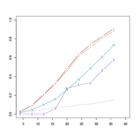
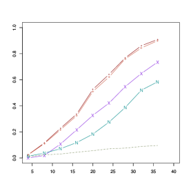
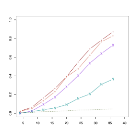
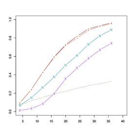
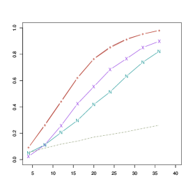
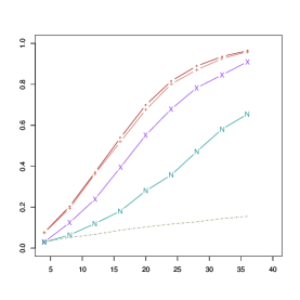
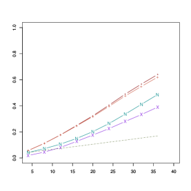
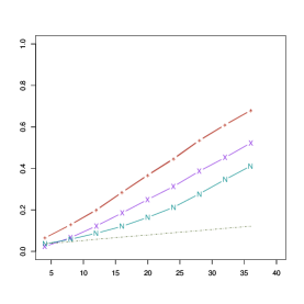
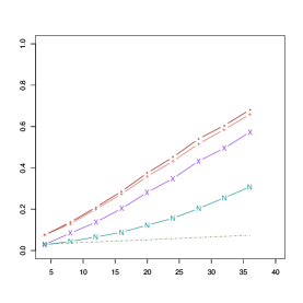
Figure 3: The performance of $\gamma=\{0,1,0.5,\gamma^{\star}\}$ according to $E[\mbox{S@1}(\gamma)]$, $\mbox{MRR}(\gamma)$, and $\mbox{MAP}(\gamma)$ (top, middle, and bottom, respectively). Columns, from left to right, represent $m^{\prime}=\frac{m}{4},\frac{m}{2},\frac{3m}{4}$. The $x$-axis represents increasing values of $m$ and the $y$-axis represents the evaluation criterion. Results are obtained via $1000$ random graphs generated according to the $\kappa(n=184,p=[0.6,0.2,0.2]^{\prime},m,s=[0.4,0.4,0.2]^{\prime};m^{\prime})$ model. As in the previous figure, lines with “X” markers denote context alone , those with “N” markers denote content alone, those with “+” markers denote $\gamma=0.5$ and those with “*” markers denote $\gamma=\gamma^{\star}$. The dashed line with no markers denotes chance performance.

Figure 3 generalizes the results presented in Figure 2, presenting performance as we vary $m^{\prime}$ (the proportion of $m$ with observed attributes) for all three of our evaluation criteria. Again, for small $m$, all perform equally poorly (approximately chance). As we vary the ratio of $m$ to $m^{\prime}$, we see that $T^{0.5}$ again is superior to either $T^{1}$ or $T^{0}$ alone in some cases ($m^{\prime}=\frac{m}{4},\frac{m}{2}$), but $T^{0}$ is superior to $T^{1}$ and $T^{0.5}$ in other cases ($m^{\prime}=\frac{3m}{4}$). (Chance, indicated by the dashed green line, is not the same throughout Figure 3, since we fix $n$ but vary $m^{\prime}$: the number of correct answers left in the candidate set $\mathcal{M}\setminus\mathcal{M}^{\prime}$, from left to right, is $\frac{3m}{4}$, $\frac{m}{2}$, $\frac{m}{4}$. The performance of $T^{1}$ changes across plots only because of these variations in chance performance.)

Figure 4: The colors/contours of this plot denote $\mbox{AP}^{y}(\gamma)$, with the $y$-axis representing $y$ and the $x$-axis representing $\gamma$. Note that $\gamma^{\star}$ (for all $y$ under consideration in this plot) is found near $0.4$, as indicated by the increase in $\mbox{AP}^{y}(\gamma)$ in that region. Results are obtained via $1000$ Monte Carlo replicates.

Figure 4 generalizes the results presented in Figure 2, by showing performance (measured in average precision) as a function of $\gamma$, with $\gamma$ free to vary from $[0,1]$. Let $k$ be the integer such that $V^{\gamma}_{(k)}$ is the $y^{\mbox{th}}$ highest ranked true but unknown red vertex, then

$$\mbox{AP}^{y}(\gamma)={\frac{\displaystyle\sum_{i=1}^{k}\mathbb{I}\{v^{\gamma}_{(i)}\in\mathcal{M}\setminus\mathcal{M}^{\prime}\}Pre(i,\gamma)}{y}}.$$ (10)

For example, if we are to correctly identify $y=3$ true but unknown reds, then $\mbox{AP}^{3}(0.1)\cong 0.9$ and $\mbox{AP}^{3}(0.8)\cong 0.8$; For $y=5$, $\mbox{AP}^{(}0.1)\cong 0.8$ and $\mbox{AP}^{3}(0.8)\cong 0.7$ Observe that $\gamma^{\star}\in(0,1)$, rather than $\{0,1\}$, indicating that the fusion of content and context can provide superior inferential power.

Thus we have demonstrated that fusion of content and context can be most effective, but is not always so. We also have shown that the relative performance of content, context, and fusion depend upon $m$ and $m^{\prime}$. Further results, omitted for brevity, demonstrate that performance also depends on $n$, $p$ and $s$; furthermore, even when fixing $p$, $s$, and $m^{\prime}$, there are scenarios where content is equal to, better than, and worse than context; likewise, when $p$, $s$, and $m-m^{\prime}$ are fixed. So the relative performance of content and context depends on more than the simple relationship between $m$ and $m^{\prime}$. These relative performance phenomenon are present regardless of evaluation criteria.

5 Experiments with Observed Graphs

We address three questions in this section: (1) Do the phenomena described by our assumptions from Section 2 naturally occur? (2) If and when these phenomena do occur, is the vertex nomination procedure laid out in Section 3 a viable approach to uncover occluded vertices? (3) If and when these phenomena do occur and the vertex nomination procedure is viable, is it better to use context information alone ($\gamma=0$), content information alone ($\gamma=1$) or a linear fusion of the two ($\gamma\in(0,1)$)?

Simulations provide useful insight into how vertex nomination performs when the phenomenon of interest is generated according to a model based on our assumptions and limited understanding of the underlying social phenomena (Section 4). Our simulations do not purport to capture all the salient aspects of the human-generated behavior that gives rise to the set of emails in our corpus. Thus, to investigate the efficacy of vertex nomination beyond our generative model, we use importance sampling to discover naturally occurring examples of the phenomena of interest. We then demonstrate that vertex nomination works for these naturally occurring phenomena. We consider partitions of $V$ which satisfy our assumptions (from Section 2), and estimate the parameters of a $\kappa$ graph model, for comparison to results from the generative model. Note that these are estimates of the parameter values from real data, rather than set parameter values.

5.1 Importance Sampling

We obtain a communications graph from the Enron email corpus; $V$ is comprised of $n=184$ vertices (email addresses), and edges connect pairs of vertices that communicate at least once during a specific 20 week time period ($E_{Enron}$). We consider Enron graph $G_{Enron}=(V,E_{Enron})$. (See Appendix for further details.)

We augment $G_{Enron}$ with edge-topics in $\{1,\cdots,32\}$ obtained from Berry et al., (2007). We fix $m=10$ and $m^{\prime}=5$ for this section. Given $m$, we randomly select a candidate set $\mathcal{M}\subset V$. We then evaluate the appropriateness of the disjoint partition $(\mathcal{M},V\setminus\mathcal{M})$ in terms of our two assumptions from Section 2: the first requires that the frequency of communications among pairs of vertices in $\mathcal{M}$ be higher than the frequency for other pairs, and the second requires a differential in topic distribution. Toward this end, we consider for Assumption 1

$$\Delta\rho=\rho(\Omega(\mathcal{M}))-\rho(\Omega(V\setminus\mathcal{M}))$$ (11)

where $\Omega(V^{\prime})$ is the subgraph in $G=(V,E)$ induced by the subset of vertices $V^{\prime}\subset V$ and the relative density of a graph $G=(V,E)$, $\rho(G)$, is defined as

$$\rho(G(V,E))=\frac{|E|}{{{|V|}\choose{2}}}.$$

For Assumption 2, we consider

$$\Delta P=||P(\Omega(\mathcal{M}))-P(\Omega(V\setminus\mathcal{M}))||_{1}$$ (12)

where the vector $P(G)=[P_{1}(G),\cdots,P_{32}(G)]$ is the empirical distribution of edge-topics. Thus $\Delta P$ represents the differential in topic distribution between $\mathcal{M}$ and $V\setminus\mathcal{M}$. In the Enron collection, edges often represent multiple messages between the two email addresses, so for any edge $e$ we induce a probability distribution $\mathscr{T}_{e}$ over Berry topics $\{1,\cdots,32\}$ from the observed messages; note that for $e=uv$, $\mathscr{T}_{e}$ is just $P(\Omega(\{u,v\}))$.

Given the Enron graph $G_{Enron}=(V,E_{Enron})$ and specified $m$ and $m^{\prime}$, our importance sampling proceeds as follows:

1. Randomly partition the vertices into $\mathcal{M}$ and $V\setminus\mathcal{M}$.

2. If either $\Delta\rho\leq\tau_{\rho}$ or $\Delta P\leq\tau_{P}$ then discard this $(\mathcal{M},V\setminus\mathcal{M})$ partition and restart, where $\tau_{\rho}$ and $\tau_{P}$ are somewhat arbitrarily specified thresholds.

3. Otherwise,

   Label the vertices in $\mathcal{M}$ $red$ ($\phi_{V}(v)=1$ for $v\in\mathcal{M}$);

   Label the vertices in $V\setminus\mathcal{M}$ $green$ ($\phi_{V}(v)=2$ for $v\in V\setminus\mathcal{M}$);

   Define a mapping $\mathscr{M}$ from topic number $\{1,\cdots,32\}$ to attribute $\{red,green\}$ by letting $\Delta P_{k}=P_{k}(\Omega(\mathcal{M}))-P_{k}(\Omega(V\setminus\mathcal{M}))$ for each topic $k$ and if $\Delta P_{k}>0$, $\mathscr{M}(k)=1$ ($red$); otherwise $\mathscr{M}(k)=2$ ($green$).

From this importance-sampling procedure, we have a set of acceptable vertex partitions $(\mathcal{M},V\setminus\mathcal{M})$ and corresponding mappings from Berry topics to $red$ or $green$ attributes ($\mathscr{M}$). For each acceptable partition-map pair, we perform Monte Carlo experiments by instantiating each edge with a single Berry-topic, according to its topic distribution, and proceeding with vertex nomination according to the following procedure:

1. Draw a topic $T_{e}$ for edge $e$ according to its distribution over Berry topics $\mathscr{T}_{e}$.

2. Attribute each edge $e\in E$ with $\mathscr{M}(T_{e})$ ($\phi_{E}(e)=\mathscr{M}(T_{e})$).

3. Thus, $G(V,E,\phi_{V},\phi_{E})$.

4. Randomly select $\mathcal{M}^{\prime}$ from $\mathcal{M}$ to be the vertices with observed vertex-attributes; occlude attributes on the rest of the vertices ($V\setminus\mathcal{M}^{\prime}$).

5. Thus, $G^{\prime}(V,E,\phi_{V},\phi_{E},\mathcal{M}^{\prime})$.

6. Perform vertex nomination.

From an observed graph obtained by the procedure described above (both importance sampling and instantiation), we obtain estimates $\hat{{p}}$ and $\hat{{s}}$ by counting the proportion of the possible edges that exist and have the appropriate attribute:

$$\hat{{p}}_{1}=\frac{|\{e\in E(\Omega(V\setminus\mathcal{M})):\phi_{E}(e)=1\}|}{{{n-m}\choose{2}}},\hat{{p}}_{2}=\frac{|\{e\in E(\Omega(V\setminus\mathcal{M})):\phi_{E}(e)=2\}|}{{{n-m}\choose{2}}}$$

and

$$\hat{{s}}_{1}=\frac{|\{e\in E(\Omega(\mathcal{M})):\phi_{E}(e)=1\}|}{{{m}\choose{2}}},\hat{{s}}_{2}=\frac{|\{e\in E(\Omega(\mathcal{M})):\phi_{E}(e)=2\}|}{{{m}\choose{2}}}.$$

For $\tau_{P}>0$ and $\tau_{\rho}>0$, this results in real Enron data attributed graphs satisfying (probabilistically) Assumptions 1 and 2.

5.2 Results for Enron Experiments

Fusion of content and context generally yields an improvement over either content or context alone, as shown in Figures 5 and 7.

Figure 5 reveals, as expected, that the performance for $\gamma=0$ depends on $\Delta\rho$: as the $\mathcal{M}$ are more interconnected than are the $V\setminus\mathcal{M}$, the probability of nominating a vertex from $\mathcal{M}\setminus\mathcal{M}^{\prime}$ instead of $V\setminus\mathcal{M}$ increases. Also, the performance for $\gamma=0$ is largely independent of $\Delta P$. Contrary to intuition, perhaps, the performance of $\gamma=1$ is not wholly dependent upon $\Delta P$ nor entirely independent of $\Delta\rho$, due to the fact that the content signal depends on excess interesting content which is not independent of the probability of edges themselves. Figure 8 shows results comparable to plots from other sections, as estimated from the importance-sampled observed graphs.

Figure 5: Content (’N’), context (’X’), arbitrary linear fusion (’+’) and optimal linear fusion (’*’) ($\gamma=\{0,1,0.5,\gamma^{\star}\}$ respectively) according to $\mbox{MAP}(\gamma)$ on importance-sampled graphs, plotted on the $y$-axis. Left: MAP ($y$-axis) and $\Delta\rho$ ($x$-axis), conditioned on a small range of $\Delta P\in[0.2,0.3]$. Right: MAP ($y$-axis) and $\Delta P$ ($x$-axis), conditioned on a small range of $\Delta\rho\in[0.3,0.4]$. In all cases, the average reported reflects at least 20 partitions. Chance is denoted by the dashed green line.

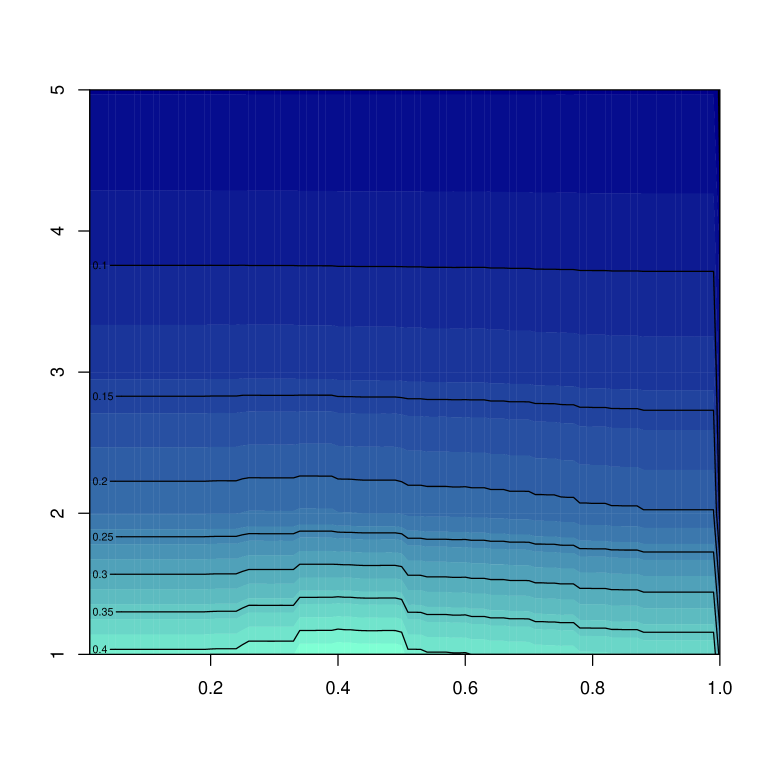
Figure 6: The colors/contours of this plot denote $\mbox{AP}^{y}(\gamma)$, with the $y$-axis representing $y$ and the $x$-axis representing $\gamma$. Note that $\gamma^{\star}$ (for all $y$ under consideration in this plot) is found near $0.4$, as indicated by the increase in $\mbox{AP}^{y}(\gamma)$ in that region.

Figure 6 generalizes the results presented in Figure 5, by showing performance (measured in average precision) as a function of $\gamma$, as $\gamma$ varies from $[0,1]$, for the importance sampled partitions present in a small range of $\Delta\rho$ and $\Delta P$. Observe that $\gamma^{\star}$ is found for $\gamma\in(0,1)$, rather than $\gamma\in\{0,1\}$, indicating that non-trivial fusion of content and context provides superior inferential power for this range of $\Delta\rho$ and $\Delta P$.

Figure 7: The difference in performance across the joint space of $\Delta\rho$ and $\Delta P$ between additive fusion and content or context. Specifically, we plot $\min(\mbox{MRR}(\gamma=0),\mbox{MRR}(\gamma=1))-\mbox{MRR}(\gamma=0.5)$ for each $(\Delta\rho,\Delta P)$. The $x$-axis shows $\Delta\rho$ and the $y$-axis shows $\Delta P$. White indicates regions where there were an insufficient number of observed samples to reliably calculate performance ($<20$). Purple regions indicate that the performance at $\gamma=0.5>\gamma\in\{0,1\}$ and cyan regions indicate that performance at $\gamma=0>\gamma\in\{0.5,1\}$. Thus, purple indicates regions where fusion helps, cyan indicates regions where fusion hurts, and white indicates regions where there is not enough data for a conclusive estimate. White should also be interpreted as configurations that are highly unlikely, given the number of samples investigated.

Figure 7 explores the differences between $T^{\gamma^{\star}}$ and $T^{0}$ or $T^{1}$ respectively, indicating where the performance obtained by fusing content and context is greater than using either alone. Where Figure 6 reports results for a small range of $\Delta\rho$ and $\Delta P$, Figure 7 reports results for many such small regions (Figure 6 covers only one cell reported in Figure 7). Over almost all the observed graphs obtained by the importance sampling procedure, $T^{\gamma^{\star}}$ is superior to either $T^{0}$ or $T^{1}$.

$\hat{p}_{1}$	$\hat{p}_{2}$
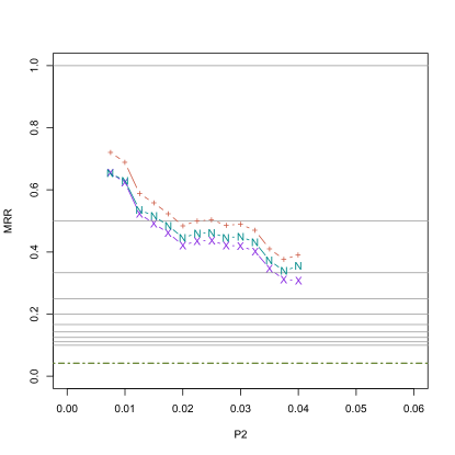
$\hat{s}_{1}$	$\hat{s}_{2}$

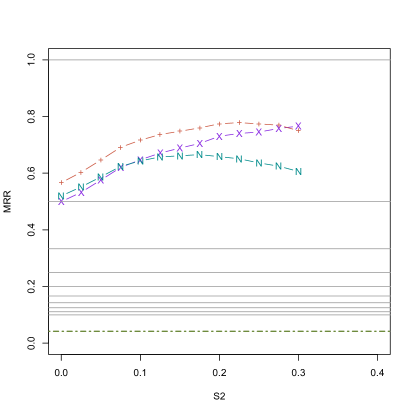
Figure 8: $\mbox{MRR}(\gamma)$ (on the $y$-axis) for $\gamma\in\{0,0.5,1\}$ for importance sampled graphs according to the estimated vectors $\hat{p}$ (top) and $\hat{s}$ (bottom). The $x$-axis denotes the estimated proportion of topic 1 (of interest) in the left column and topic 2 (not of interest) in the left column. In all cases, the average reported reflects at least 20 partitions. Chance is denoted by the dashed green line.

In sum, we do find (1) that the phenomena of interest do naturally occur, (2) that when they do occur vertex nomination is viable, and (3) the fusion of content and context (arbitrary, $\gamma=0.5$ and optimal, $\gamma=\gamma^{\star}$) is superior to either alone for vertex nomination when these phenomena naturally occur.

6 Conclusion

In this investigation we explore vertex nomination – finding interesting vertices – using information from context (graph structure) and content (edge-attributes). We present simulation and experimental results supporting the intuition that content and context are often better together than either alone, for this task.

We present only simple linear content and context fusion statistics, in an effort to demonstrate the fundamental superiority of non-trivial fusion. There is much room for more complex and better performing content, context, and fusion statistics. We leave this area open to future research.

Results on real data are, by necessity, subjective for at least two reasons. For one, the definition of “interesting” is likely to change significantly between datasets (and indeed those examining the datasets). Secondly, the relationship between the mathematical model ($\kappa$) and the observed behavior (and the effects thereof) is not easily quantified, so performance cannot be easily predicted a priori. For illustrative purposes, we present results for one dataset (with one definition of interesting) using the Enron corpus, though application and adaptation to new datasets (with different interesting phenomena, behavior of vertices, and parameter values) remains an interesting and open question.

Knowledge of the relationships between performance and parameter values provides useful information about the robustness and generalization of the techniques beyond the simple setting explored. Specifically, these relationships can be exploited when applying these (or similar) techniques to real data, where analogs of the parameters can be estimated.

Appendix A: Enron Email Corpus

The Enron email corpus, used in this investigation, is a collection of emails seized by the Securities and Exchange Commission (SEC) during their investigation into potentially fraudulent and manipulative behavior of some Enron employees. Copies of all emails in the accounts of some 150 employees were obtained (both send and received messages) and eventually released to the public. We work with an approximately 27,000 message subset of the 500,000 email messages seized (though some are duplicates found in the inbox of many individuals), for comparison across studies (e.g. Priebe et al., (2005), Coppersmith et al., (2011)) The emails in the subset are those for which both the sender and the receiver is on of a list of 184 employees present in an organizational-heirarchy chart (mostly executives, traders, and secretaries). From this collection, we select an arbitrary 20 week period, from September 24, 2001 to February 11, 2002, to examine.

Let $G_{Enron}=(V_{Enron},E_{Enron})$, where $v\in V_{Enron}$ is an email address corresponding to one of the 184 employees mentioned above. $|V_{Enron}|=n_{Enron}$. If an email exists in the time period under consideration between $i,j\in V_{Enron}$, then $ij\in E_{Enron}$. Approximately 5 percent of the ${n_{Enron}}\choose{2}$ possible edges exist, so $\hat{p}_{Enron}=0.05$.

A subset of emails (overlapping but different from that above) was labeled by topic by Michael Berry, Berry et al., (2007). Bennett Landman, Tamer El-Sayed and Douglas Oard created a classifier, based on word count histograms, for these Berry-topics. The entire dataset was labeled with this classifier (including those originally labeled by Berry, for consistency). These topic labels are used throughout this investigation.

In fact, we treat each (undirected) edge $ij$ as the collection of messages exchanged between $i$ and $j$ during the time period. This gives rise to our representation of each edge as a distribution over topics, since each email has a topic associated with it, and each edge is comprised of many emails.

References

- Bell et al., (2008) Bell, R. M., Koren, Y., and Volinsky, C. (2008). The bellkor solution to the netflix prize. Available from Available from www.netflixprize.com.
- Berry et al., (2007) Berry, M. W., Browne, M., and Signer, B. (2007). 2001 topic annotated enron email data set.
- Bollobás, (2001) Bollobás, B. (2001). Random Graphs. Cambridge University Press, Cambridge, second edition.
- Buckley and Voorhees, (2005) Buckley, C. and Voorhees, E. M. (2005). Retrieval System Evaluation. In Voorhees, E. M. and Harman, D. K., editors, TREC: Experiment and Evaluation in Information Retrieval, pages 53–75. MIT Press.
- Coppersmith et al., (2011) Coppersmith, G. A., Marchette, D. J., Rukhin, A., and Priebe, C. (2011). Statistical Inference on Graphs: Estimation Anomaly Characteristics. In Progress.
- Cortes et al., (2002) Cortes, C., Pregibon, D., and Volinsky, C. (2002). Communities of interest. Intelligent Data Analysis, 6(3):211.
- Priebe et al., (2005) Priebe, C. E., Conroy, J. M., Marchette, D. J., and Park, Y. (2005). Scan statistics on enron graphs. Computational and Mathematical Organization Theory, 11:229–247.
- (8) Priebe, C. E., Coppersmith, G. A., and Rukhin, A. (2010a). You say graph invariant, i say test statistic. ASA Sections on Statistical Computing Statistical Graphics SCGN Newsletter, 21(2):11–14.
- (9) Priebe, C. E., Park, Y., Marchette, D. J., Conroy, J. M., Grothendieck, J., and Gorin, A. L. (2010b). Statistical inference on attributed random graphs: Fusion of graph features and content: An experiment on time series of enron graphs. Computational Statistics & Data Analysis, 54(7):1766 – 1776.
- Resnick and Varian, (1997) Resnick, P. and Varian, H. R. (1997). Recommender systems. Commun. ACM, 40:56–58.