Analysis of Cell Load Coupling for LTE Network Planning and Optimization

Abstract

System-centric modeling and analysis are of key significance in planning and optimizing cellular networks. In this paper, we provide a mathematical analysis of performance modeling for LTE networks. The system model characterizes the coupling relation between the cell load factors, taking into account non-uniform traffic demand and interference between the cells with arbitrary network topology. Solving the model enables a network-wide performance evaluation in resource consumption. We develop and prove both sufficient and necessary conditions for the feasibility of the load-coupling system, and provide results related to computational aspects for numerically approaching the solution. The theoretical findings are accompanied with experimental results to instructively illustrate the application in optimizing LTE network configuration.

I Introduction

Planning and optimization of LTE network deployment, such as base station (BS) location and antenna parameter configuration, necessitate modeling and algorithmic approaches for network-level performance evaluation. Finding the optimal network design and configuration amounts to solving an optimization problem of combinatorial nature. Toward this end, system modeling admitting rapid performance assessment in order to facilitate the selection among candidate configuration solutions, of which the number is typically huge, is essential. In this paper, we provide a rigorous analysis of an LTE system performance model that works for general network topology and explicitly accounts for non-uniform traffic demand. The performance model that we study is referred to as the load-coupling system, to emphasize the fact that the model characterizes the coupling relation between the cells in their load factors. For each cell, the load factor is defined as the amount of resource consumption in relation to that is available in the cell. The load value grows with the cell’s traffic demand and the amount of inter-cell interference. Intuitively, low load means that the network has more than enough capacity to meet the demand, whilst high load indicates poor performance in terms of congestion and potential service outage. In the latter case, the network design and configuration solution in question should be revised, by reconfiguration or adding BS infrastructure. Thus, simple means for evaluating the cell load for a given candidate design solution is of high importance, particularly because the evaluation may have to be conducted for a large number of user demand and network configuration scenarios.

The load-coupling model for LTE networks takes the form of a non-trivial system of non-linear equations. Calculating the solution to the model, or determining solution existence, is not straightforward. In this paper, we present contributions to characterizing and solving the load-coupling system model. First, we present a rigorous mathematical analysis of fundamental properties of the system and its solution. Second, we develop and prove a sufficient and necessary condition for solution existence. Third, we provide theoretical results that are important for numerically approaching the solution or delivering a bounding interval. Fourth, we instructively illustrate the application of the system model for optimizing LTE network configuration.

The remainder of the paper is organized as follows. In Section II we review some related works. The system model is presented in Section III, and its fundamental properties are discussed in Section IV. In Section V, we present linear equation systems for the purpose of determining solution existence. In Section VI, we provide the relation between solving the load-coupling system and convex optimization, and discuss approximate solutions. The application of the system model and our theoretical results to LTE network optimization is illustrated in Section VII, and conclusions are given in Section VIII.

II Related Works

Planning and performance optimization in cellular networks form a very active line of research in wireless communications. There are many works on UMTS network planning and optimization. The research topics range from BS location and coverage planning [3, 4, 5, 25, 43], antenna parameter configuration [16, 15, 33], to cell load balancing [18, 34]. For UMTS, the power control mechanism that links together the cells in resource consumption is an important aspect in performance modeling [2, 3, 19, 41, 42]. By power control, the transmit power of each link is adjusted to meet a given signal-to-interference-and-noise ratio (SINR) threshold. By the SINR requirement, the power expenditure of one cell is a linear function in those of the other cells. As a result, the power control mechanism is represented by a system of linear equations, which sometimes is referred to as UMTS interference coupling [16, 15]. Interference coupling can be modeled for both downlink and uplink. For network planning, the interference coupling system needs to be solved many times for performance evaluation of different candidate network configurations and multiple or aggregate user demand snapshots. In [26], it is shown that, for both downlink and uplink radio network planning, the dimension of the power-control-based system of equations can be reduced from the number of users in the system to the number of cells. The observation stems from system characteristics that also form the foundation of distributed power control mechanisms, see, e.g., [19, 42]. In [12], the authors provide theoretical properties of the power-control-based system, and feasibility conditions in terms of target data rates and QoS requirements. Motivated by the fact that full-scale dynamic simulation is not computationally affordable for large networks, the authors of [44] extend the UMTS power-control system by a randomization-based procedure of service and rate adaptation for HSUPA network planning.

In cellular network planning, the power-control equation system is considered under given SINR threshold. Thus the system solution and its existence are induced by the (candidate) network configuration in question. In a more general context of wireless communications, power control is often a means in performance optimization, that is, the powers are optimization variables in minimizing or maximizing objectives representing error probability, utility, QoS, etc., that are all functions of SINR. There is a vast amount of theoretical analysis and algorithmic approaches for power optimization under various (typically non-linear) objective functions, where a gain matrix defines interference coupling [38, 37, 39, 40]. In [37], the authors identify objective functions admitting a convex formulation of power optimization, and develop a distributed gradient-projection-based algorithm. Further developments include algorithmic design utilizing Kuhn-Tucker condition [39], conditional Newton iteration yielding quadratic convergence [40], and model extension to include explicit SINR-threshold constraints [38].

Another line of research of power control is the characterization of the achievable performance region under various utility functions and interference functions. The authors of [11] show the strict convexity of the region for logarithmic functions of SINR. In [7], the authors characterize utility functions and function transformation of power, for which the resulting power optimization problem is convex. The investigation in [9] provides conditions under which the boundary points of the region are Pareto-optimal. In [8], the authors present graph representations of power and interference, and study the relation between graph structure, irreducibility of the interference coupling matrix, and the convexity of the utility region.

In contrast to the power-control model, the service requirement of rate-control scheme in cellular networks is not SINR threshold (or a function of SINR), but the amount of data to be served over a given time period. Among other advantages, this approach makes it possible to capture the effect of scheduling without the need of explicitly modeling full details of scheduling algorithms. The rate-control-based approach is primarily targeting, although not limited to, non-power-controlled systems or systems with a fixed-rate traffic demand. The approach has been less studied, but is of a high interest for OFDMA-based networks. In general, the rate-control scheme exhibits non-linear relations between the cell-coupling elements (in our case, cell loads). The resulting model is therefore more complex than the power-control model for UMTS. For power control, fundamental solution characterizations are well-established for linear as well as more general interference functions. For the latter, see, for example, [10]. For rate-control-based coupling systems (see [23] and Section III), a structural difference from power control is that, in the former, one element cannot be expressed as a sum of terms, each being a function denoting the impact of another element, and the coupling is not scale invariant. For network planning, one known approach is to consider an approximate linear function, obtained from system-specific adaptive modulation and coding (AMC) parameters, to represent the relation between date rate and SINR [24], and thereby arrive at a equation system being similar to that of UMTS.

From an engineering standpoint, LTE network optimization is becoming increasingly important. In [13], the authors provide the fundamental principles of LTE network operation and radio resource allocation. Among the optimization issues, the research theme of scheduling strategies and radio resource management (RRM) algorithms has been extensively investigated. See, for example, [6, 20, 22, 21, 29, 30, 31] and the references therein. Two major aspects considered in the references are the balance between resource efficiency and fairness, and quality of service awareness. In [17], the author gives a survey of tools enabling service and subscriber differentiation. For cell planning, the propagation modeling, link budget consideration, and performance parameters have been investigated in [36].

High-level and accurate performance modeling is of high value in planning cellular networks, as full-scale dynamic simulations are not affordable for large planning scenarios (e.g., [44]). The LTE system model that we analyze has been introduced by Siomina et al. [32] for studying OFDM network capacity region with QoS consideration. The work in [32] does not, however, provide a general analysis of the model, and the major part of the study relies on a simplification assuming uniform load among cells. In the forthcoming sections, we present both analytical and numerical results without these limitations.

Recently, the authors of [23] have presented a non-linear LTE performance model being very similar to the one studied in the current paper. That our performance model has been independently proposed by others supports the modeling approach. The work in [23] provides further an approximation of load coupling via another non-linear but simpler equation system, along with incorporating continuous user distribution. Our study differs from [23], as the focus of the current paper is a detailed investigation of key properties and solution characterization of the load coupling system.

III The System Model

Denote by $\mathcal{N}=\{1,\dots,n\}$ the set of cells in a given network design solution. Without loss of generality, we assume that each cell has one antenna to simplify notation. The service area is represented by a grid of pixels or small areas, each being characterized by uniform signal propagation conditions. The set of pixels is denoted by $\mathcal{J}$. The total power gain between antenna $i$ and pixel $j$ is denoted by $g_{ij}$. We use $\mathcal{J}_{i}\subset\mathcal{J}$ to denote the serving area of cell $i$. In a network planning context, both the gain matrix as well as the cells’ serving areas are determined by BS location and antenna configuration.

For realistic network planning scenarios, the traffic demand is irregularly distributed. Let the user demand in pixel $j$ be denoted by $d_{j}$. The demand represents the amount of data to be delivered to the users located in pixel $j$ within the time interval under consideration. By defining a service-specific index, the demand parameter and the system model can be extended to multiple types of services (see [32]). We will, however, consider one service type merely for the sake of compactness.

We use $\rho_{i}$ to denote the level of resource consumption in cell $i$. The entity is also referred to as cell load. In LTE systems, the cell load can be interpreted as the expected fraction of the time-frequency resources that are scheduled to deliver data. The network-wise load vector, ${\boldsymbol{\rho}}=(\rho_{1},\rho_{2},\dots,\rho_{n})^{T}$, plays a key role in performance modeling. In particular, a well-designed network shall be able to meet the target demand scenarios without overloading the cells. Hence the load vector forms a natural performance metric in network configuration (cf. power consumption in UMTS networks). The load of a cell is a result of the user demands in the pixels in the cell serving area, the channel conditions, as well as the amount of interference. The last aspect inter-connects the elements in the load vector, as the load of a cell is determined by the SINRs and the resulting bit rates over the cell’s serving area, and these values are in turn dependent on the load values of the other cells. To derive the performance model, we consider the SINR in pixel $j\in\mathcal{J}_{i}$ defined as follows,

$$\gamma_{j}({\boldsymbol{\rho}})=\frac{P_{i}g_{ij}}{\displaystyle\sum_{k\in\mathcal{N}\setminus\{i\}}P_{k}g_{kj}\rho_{k}+\sigma^{2}}.$$ (1)

In (1), $P_{i}$ is the power spectral density per minimum resource unit in scheduling (in LTE, this corresponds to a pair of time-consecutive resource blocks), and $\sigma^{2}$ is the noise power. By (1), the inter-cell interference grows by the load factor. In effect, $\rho_{k}$ can be interpreted as the probability of receiving interference originating from cell $k$ on all the sub-carriers of the resource unit. Let $B\log_{2}(1+\gamma_{j}({\boldsymbol{\rho}}))$ be a function describing the effective bitrate per resource unit. This formula is shown to be very accurate for LTE downlink [27]. Thus to serve demand $d_{j}$ in $j$, $\frac{d_{j}}{B\log_{2}(1+\gamma_{j}({\boldsymbol{\rho}}))}$ resource units are required.

Let $K$ denote the total number of resource units in the frequency-time domain in question, and denote by $\rho_{ij}$ the proportion of resource consumption of cell $i$ due to serving the users in $j\in\mathcal{J}_{i}$. By these definitions, we obtain the following equation,

$$K\rho_{ij}=\frac{d_{j}}{B\log_{2}(1+\gamma_{j}({\boldsymbol{\rho}}))}.$$ (2)

From (2), it is clear that the load of a cell is a function of the load levels of other cells. Observing that $\rho_{i}=\sum_{j\in\mathcal{J}_{i}}\rho_{ij}$ and putting the equations together lead to the following equation,

$$\rho_{i}=\sum_{j\in\mathcal{J}_{i}}\rho_{ij}=\sum_{j\in\mathcal{J}_{i}}\frac{d_{j}}{KB\log_{2}(1+\gamma_{j}({\boldsymbol{\rho}}))}=\sum_{j\in\mathcal{J}_{i}}\frac{d_{j}}{KB\log_{2}\left(1+\frac{P_{i}g_{ij}}{\sum_{k\in\mathcal{N}\setminus\{i\}}P_{k}g_{kj}\rho_{k}+\sigma^{2}}\right)}~{}.$$ (3)

The equation above represents the coupling relation between cells in their resource consumption. In vector form, we have ${\boldsymbol{\rho}}={\boldsymbol{f}}({\boldsymbol{\rho}},{\boldsymbol{g}},{\boldsymbol{d}},K,B)$, where ${\boldsymbol{f}}=(f_{1},\dots,f_{i},\dots,f_{n})^{T}$, and $f_{i},i=1,\dots,n$, represents the $\mathbb{R}_{+}^{n-1}\rightarrow\mathbb{R}_{+}$ function as defined by (3); here, $\mathbb{R}_{+}$ and $\mathbb{R}_{+}^{n-1}$ are used to denote the single- and $(n-1)$-dimension space of all real non-negative numbers, respectively. Since in the subsequent discussions there will be no ambiguity in the input parameters, we use the following compact notation to denote the non-linear equation system,

$${\boldsymbol{\rho}}={\boldsymbol{f}}({\boldsymbol{\rho}}).$$ (4)

From (3), three immediate observations follow. First, for all $i=1,\dots,n$, the load function $f_{i}$ is strictly increasing in the load of other cells. Second, for non-zero $\sigma^{2}$, this function is strictly positive when the load values of other cells (and thus interference) are all zeros, i.e., ${\boldsymbol{f}}(0)>0$. Third, the function is continuous, and at least twice differentiable for ${\boldsymbol{\rho}}\geq 0$.

From the network performance standpoint, the capacity is sufficient to support the traffic demand, if equation system (4) admits a load vector ${\boldsymbol{\rho}}$ with $0\leq\rho_{i}\leq 1,i\in\mathcal{N}$. In our analysis, however, we do not restrict ${\boldsymbol{\rho}}$ to be at most one, in order to avoid any loss of generality. In addition, even if the solution contains elements being greater than one, the values are of significance in network planning, because they carry information of the amount of shortage of resource in relation to the demand.

Solving (4) deals with finding a fixed point (aka invariant point) of function ${\boldsymbol{f}}$ in $\mathbb{R}^{n}_{+}$, or determines that such a point does not exist. In the remainder of the paper, we use $S$ as a general notation for the space of non-negative solutions (fixed points) to systems of equations or inequalities. The system in question is identified using subscript. Thus, $S_{{\boldsymbol{\rho}}={\boldsymbol{f}}({\boldsymbol{\rho}})}$ denotes the solution space of (4). Note that, for (4) as well as the linear equation systems to be introduced later, only non-negative solutions are of interest. Hence, throughout the article, a (linear or non-linear) system is said to be feasible, if there exists a solution for which non-negativity holds, otherwise the system is said to be infeasible (even if a solution of negative values exists). The case that (4) is infeasible is denoted by $S_{{\boldsymbol{\rho}}={\boldsymbol{f}}({\boldsymbol{\rho}})}=\emptyset$.

A useful optimization formulation in our analysis is the minimization of the total cell load, subject to the inequality form of (4). The formulation is given below.

$$\min~{}~{} \sum_{i\in{\cal N}}\rho_{i}$$ (5a)

$${\boldsymbol{\rho}}\geq{\boldsymbol{f}}({\boldsymbol{\rho}})$$ (5b)

$${\boldsymbol{\rho}}\in\mathbb{R}_{+}^{n}$$ (5c)

For (5), its solution space $S_{{\boldsymbol{\rho}}\geq{\boldsymbol{f}}({\boldsymbol{\rho}})}$ is also referred to as the feasible load region. Recall that ${\boldsymbol{f}}({\boldsymbol{\rho}})$ is strictly increasing, hence if $S_{{\boldsymbol{\rho}}\geq{\boldsymbol{f}}({\boldsymbol{\rho}})}\not=\emptyset$, then for any optimal solution to (5), (5b) holds with equality, as otherwise (5a) can be improved, contradicting that the solution is optimal. In conclusion, any optimum of (5) is a solution to (4).

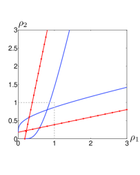
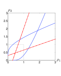
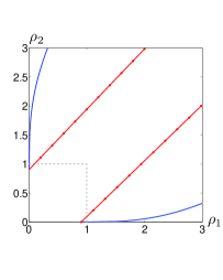
We end the section by an illustration of the load-coupling system for two cells in Figure 1. The two cells have symmetric parameters. In the figure, the two non-linear functions are given by the solid lines. In the first two cases, system (4) has solutions in ${\mathbb{R}}_{+}^{2}$, though one of them represents a solution beyond the network capacity. In the last case, the system is infeasible, as the two curves will never intersect in the first quadrant. The straight lines with markers in the figure represent linear equations related to (4). Details of these linear equations are deferred to Section V.

IV Fundamental Properties

In this section, we present and prove some fundamental properties of the load-coupling system (4). These theoretical results are of key importance in the study of solution existence and computation. For compactness, we introduce additional notation to simplify (3) while keeping the essence of the equation. Define $a_{j}=\frac{KB}{d_{j}}$, $b_{ikj}=\frac{P_{k}g_{kj}}{P_{i}g_{ij}}$, and $c_{ij}=\frac{\sigma^{2}}{P_{i}g_{ij}}$. These parameters contain, respectively, the relation between the demand in pixel $j$ and the resource in cell $i$, the inter-cell coupling in gain between cells $k$ and $i$ in pixel $j$, and the channel quality of cell $i$ in relation to noise in pixel $j$. The load equation (3) can then be written in the following form,

$$\rho_{i}=f_{i}({\boldsymbol{\rho}}),\textrm{~{}~{}where~{}~{}}f_{i}({\boldsymbol{\rho}})=\sum_{j\in\mathcal{J}_{i}}\frac{1}{a_{j}\log_{2}(1+\frac{1}{\sum_{k\in\mathcal{N}\setminus\{i\}}b_{ikj}\rho_{k}+c_{ij}})}.$$ (6)

The first fundamental property of (4) is how fast the load of a cell asymptotically grows in the load of another cell. We formulate and prove the fact that, in the limit, the first-order partial derivative of the load function converges to a constant. For any two cells $i,k$ ($i\not=k$), $\frac{\partial\rho_{i}}{\partial\rho_{k}}$ is equal to

$$\sum_{j\in\mathcal{J}_{i}}\ln(2)\frac{b_{ikj}}{a_{j}}\frac{1}{\ln^{2}(1+\frac{1}{\sum_{h\in\mathcal{N}\setminus\{i\}}b_{ihj}\rho_{h}+c_{ij}(\boldsymbol{\rho})})(\sum_{h\in\mathcal{N}\setminus\{i\}}b_{ihj}\rho_{h}+c_{ij})^{2}(\boldsymbol{\rho})(1+\frac{1}{\sum_{h\in\mathcal{N}\setminus\{i\}}b_{ihj}\rho_{h}+c_{ij}(\boldsymbol{\rho})})}.$$ (7)

Theorem 1

$\displaystyle\lim_{\rho_{k}\rightarrow\infty}{\frac{\partial f_{i}}{\partial\rho_{k}}}=\displaystyle\sum_{j\in\mathcal{J}_{i}}\ln(2)\frac{b_{ikj}}{a_{j}}$

Proof:

Consider the component for pixel $j$ in the sum in (7), and ignore the constant multiplier $\ln(2)\frac{b_{ikj}}{a_{j}}$. Letting $u=\sum_{h\in\mathcal{N}\setminus\{i\}}b_{ihj}\rho_{h}+c_{ij}$, (7) can be written as the following expression.

$$\frac{1}{u^{2}(1+\frac{1}{u})\ln(1+\frac{1}{u})\ln(1+\frac{1}{u})} = \frac{1}{\ln(1+\frac{1}{u})^{u}\ln(1+\frac{1}{u})^{u}+\ln(1+\frac{1}{u})^{u}\ln(1+\frac{1}{u})}$$

The theorem follows then from the facts that $\lim_{u\rightarrow\infty}(1+\frac{1}{u})^{u}=e$ and $u$ is linear in $\rho_{k}$. ∎

By Theorem 1, the load of a cell increases linearly in the load of another cell in the limit, i.e., the function converges to a line in the high-load region. Moreover, the slope of the line is strictly positive.

The next fundamental property is concavity. The examples in Figure 1 indicate that the load of a cell is a strictly concave function in the other cell’s load. We show that this is generally true.

Theorem 2

For any cell $i\in\mathcal{N}$, $f_{i}$ is strictly concave for $(\rho_{i},\dots,\rho_{i-1},\rho_{i+1},\dots,\rho_{n})\in R^{n-1}_{+}$.

Proof:

Without loss of generality, consider $f_{n}$ and its $(n-1)\times(n-1)$ Hessian matrix. Let $u=\sum_{h\in\mathcal{N}\setminus\{n\}}b_{nhj}\rho_{h}+c_{nj}$. For two cells $k$ and $h$, the Hessian element has the following expression.

$$\frac{\partial^{2}f_{n}}{\partial\rho_{k}\partial\rho_{h}}=\ln(2)\sum_{j\in\mathcal{J}_{n}}\frac{b_{nkj}b_{nhj}}{a_{j}}\cdot\frac{\ln(1+\frac{1}{u})[2-(2u+1)\ln(1+\frac{1}{u})]}{[\ln^{2}(1+\frac{1}{u})(u^{2}+u)]^{2}}$$ (8)

Let $q(u)=2-(2u+1)\ln(1+\frac{1}{u})$. We show that $q(u)<0$ for $u>0$. This holds, for example, for $u=1$. Next, $\lim_{u\rightarrow\infty}q(u)=2-\lim_{u\rightarrow\infty}\ln\left[(1+\frac{1}{u})^{u}(1+\frac{1}{u})^{u}(1+\frac{1}{u})\right]$ $=0$. Consider $q^{\prime}(u)$ and $q^{\prime\prime}(u)$: $q^{\prime}(u)=-2\ln\left(1+\frac{1}{u}\right)+\frac{1}{u}+\frac{1}{u+1}$, and $q^{\prime\prime}(u)=\frac{-1}{u^{2}(u+1)^{2}}<0,\forall u>0$. Therefore $q^{\prime}(u)$ is strictly decreasing and $\lim_{u\rightarrow\infty}q^{\prime}(u)=0$. Hence, $q^{\prime}(u)>0$, meaning that $q(u)$ is strictly increasing for $u>0$. This, together with $q(1)<0$ and $\lim_{u\rightarrow\infty}q(u)=0$, prove that $q(u)<0$, $\forall u>0$. By the definition of $u$, for ${\boldsymbol{\rho}}\geq 0$, $u\geq c_{nj}$ which a strictly positive number for non-zero noise power. Hence (8) is well-defined and negative for all ${\boldsymbol{\rho}}\geq 0$. Next, observe that the Hessian matrix is the result of the following expression.

$$\sum_{j\in\mathcal{J}_{i}}\frac{(b_{n1j},\dots,b_{n(n-1)j})(b_{n1j},\dots,b_{n(n-1)j})^{T}}{a_{j}}\cdot\frac{\ln(2)\ln(1+\frac{1}{u})q(u)}{[\ln^{2}(1+\frac{1}{u})(u^{2}+u)]^{2}}$$ (9)

Because of the form of (9) and that $q(u)<0,\forall u\geq c_{nj}>0$, the Hessian matrix is negative definite for any ${\boldsymbol{\rho}}\geq 0$. Hence the conclusion. ∎

From the concavity result, it follows that, for any cell $i$, $f_{i}(\rho_{1},\dots,\rho_{i-1},\rho_{i+1},\dots,\rho_{n})-\rho_{i}$ exhibits a strict radially quasiconcave structure. A function is radially quasiconcave, if for a given stationary positive point, which is in our case a solution to $f_{i}(\rho_{1},\dots,\rho_{i-1},\rho_{i+1},\dots,\rho_{n})=\rho_{i}$, and any scalar in range $(0,1)$, the function value of the scaled point is greater than or equal to zero. If the value is positive, the function is strictly radially quasiconcave.

Corollary 3

For each $i\in\mathcal{N}$, $f_{i}(\rho_{1},\dots,\rho_{i-1},\rho_{i+1},\dots,\rho_{n})-\rho_{i}$ is strictly radially quasiconcave, i.e., if $f_{i}(\rho_{1},\dots,\rho_{i-1},\rho_{i+1},\dots,\rho_{n})=\rho_{i}$, then $f_{i}(\lambda\rho_{1},\dots,\lambda\rho_{i-1},\lambda\rho_{i+1},\dots,\lambda\rho_{n})>\lambda\rho_{i}$ for any $\lambda\in(0,1)$.

Proof:

Note that $f_{i}(\lambda(\rho_{1},\dots,\rho_{i-1},\rho_{i+1},\dots,\rho_{n}))$ $=f_{i}(\lambda(\rho_{1},\dots,\rho_{i-1},\rho_{i+1},\dots,\rho_{n})+0(1-\lambda)$. By Theorem 2, we have $f_{i}(\lambda(\rho_{1},\dots,\rho_{i-1},\rho_{i+1},\dots,\rho_{n}))>\lambda f_{i}(\rho_{1},\dots,\rho_{i-1},\rho_{i+1},\dots,\rho_{n})+(1-\lambda)f_{i}(0)$. Since $f_{i}((\rho_{1},\dots,\rho_{i-1},\rho_{i+1},\dots,\rho_{n}))=\rho_{i}$ and $f_{i}(0)>0$, the result follows. ∎

In a real-life LTE network, if the capacity is sufficient to accommodate the demand, then the network load will be at a stable working point, which should be unique. Thus the performance model ${\boldsymbol{f}}$ is reasonable only if uniqueness holds mathematically. The following theorem states this is indeed the case. In the rest of the paper, the unique solution, if it exists, is denoted by ${\boldsymbol{\rho}}^{*}$.

Theorem 4

If $S_{{\boldsymbol{f}}({\boldsymbol{\rho}})={\boldsymbol{\rho}}}\not=\emptyset$, then it is a singleton, i.e., ${\boldsymbol{f}}({\boldsymbol{\rho}})={\boldsymbol{\rho}}$ has at most one solution ${\boldsymbol{\rho}}^{*}$ in ${\mathbb{R}}_{+}^{n}$.

Proof:

Suppose there are two solutions ${\boldsymbol{\rho}}^{1}$ and ${\boldsymbol{\rho}}^{2}$, both satisfying (4), and ${\boldsymbol{\rho}}^{1}\not={\boldsymbol{\rho}}^{2}$. Let $m\in\text{argmin}_{i=1,\dots,n}\rho^{1}_{i}/\rho^{2}_{i}$, and $\lambda=\rho^{1}_{m}/\rho^{2}_{m}$. Thus $\rho^{1}_{m}=\lambda\rho^{2}_{m}$. Assume $\lambda<1$. Then by construction, $\lambda{\boldsymbol{\rho}}^{2}\leq{\boldsymbol{\rho}}^{1}$, and because ${\boldsymbol{f}}$ is strictly increasing in the domain of $\mathbb{R}_{+}^{n}$, $f_{m}(\lambda{\boldsymbol{\rho}}^{2})\leq f_{m}({\boldsymbol{\rho}}^{1})$. Also, by Lemma 3, $\lambda\rho^{2}_{m}<f_{m}(\lambda{\boldsymbol{\rho}}^{2})$, and thus $f_{m}({\boldsymbol{\rho}}^{1})>\lambda\rho_{m}^{2}$. Note that $f_{m}({\boldsymbol{\rho}}^{1})=\rho_{m}^{1}=\lambda\rho_{m}^{2}$ gives an contradiction. Therefore $\lambda>1$. Considering scaling down ${\boldsymbol{\rho}}^{1}$ with $\lambda$ instead, and applying the same line of argument, a similar contradiction is obtained. Hence the conclusion. ∎

V Determining Solution Existence and Lower Bounding

Having proven solution uniqueness, we examine the existence of ${\boldsymbol{\rho}}^{*}$, that is, whether or not (4) has a fixed point. There are a number of theorems characterizing the existence of a fixed point (e.g., Brouwer’s fixed-point theorem in topology). However, these results do not apply to (4) because, in general, the output of function ${\boldsymbol{f}}$ is not confined to a compact set in ${\mathbb{R}}^{n}_{+}$. In this section, we use a linear equation system for analyzing solution existence. To this end, we first present and prove some basic properties of the optimization formulation (5).

Theorem 5

Assume $S_{{\boldsymbol{\rho}}\geq{\boldsymbol{f}}({\boldsymbol{\rho}})}\not=\emptyset$, i.e., there exists ${\boldsymbol{\bar{\rho}}}\geq{\boldsymbol{f}}({\boldsymbol{\bar{\rho}}})>0$, then (5) has an optimal solution.

Proof:

Consider the optimization problem $\min\sum_{i\in{\cal N}}\rho_{i},{\boldsymbol{\rho}}\in{\bar{S}}$, where ${\bar{S}}=S_{{\boldsymbol{\rho}}\geq{\boldsymbol{f}}({\boldsymbol{\rho}})}\cap\{{\boldsymbol{\rho}}\leq{\boldsymbol{\bar{\rho}}}\}$. By the assumption in the theorem, ${\bar{S}}\not=\emptyset$. From the definition of $\bar{S}$, it is clear that any point being arbitrarily close to $\bar{S}$ (i.e., boundary point) is in the set, thus $\bar{S}$ is closed. In addition, $\bar{S}$ is bounded since $\bar{S}\subseteq\mathbb{R}^{n}_{+}\cap\{{\boldsymbol{\rho}}\leq{\boldsymbol{\bar{\rho}}}\}$. Hence $\bar{S}$ is compact, and the result follows from Weierstrass theorem in optimization. ∎

Corollary 6

If there exists ${\boldsymbol{\bar{\rho}}}\geq{\boldsymbol{f}}({\boldsymbol{\bar{\rho}}})>0$, then $S_{{\boldsymbol{\rho}}={\boldsymbol{f}}({\boldsymbol{\rho}})}\not=\emptyset$.

Proof:

Follows immediately from Theorem 5 and the previously made observation that any optimal solution to (5) satisfies (5b) with equality. ∎

To further characterize solution existence, we define the following type of linear equation systems,

$${\boldsymbol{\rho}}={\boldsymbol{h}}({\boldsymbol{\rho}})={\boldsymbol{H}}\cdot({\boldsymbol{\rho}}-{\boldsymbol{\widehat{\rho}}})+{\boldsymbol{f}(\widehat{\boldsymbol{\rho}})},$$ (10)

where ${\boldsymbol{h}}=(h_{1},\dots,h_{n})$ is a vector of linear functions, and each of them is defined in ${\mathbb{R}}^{n-1}_{+}\rightarrow{\mathbb{R}}_{+}$, ${\boldsymbol{\widehat{\rho}}}$ is a vector in ${\mathbb{R}}^{n}_{+}$ with given values, and ${\boldsymbol{f}(\widehat{\boldsymbol{\rho}})}$ is a vector-function with elements defined by (6). In (10), ${\boldsymbol{H}}$ is an $n\times n$ matrix where the diagonal elements, $H_{ii},i=1,\dots,n$ are zeros, and the other elements $H_{ik},i\not=k$, are strictly positive. Note that if ${\boldsymbol{H}}$ is the Jacobian of function ${\boldsymbol{f}}$ evaluated at point ${\boldsymbol{\widehat{\rho}}}$, (10) is a linearization of the non-linear equation system (4) where the right-hand side of (10) represents the tangent hyperplane to function ${\boldsymbol{f}({\boldsymbol{\rho}})}$ at $\widehat{\boldsymbol{\rho}}$. Such linear approximations are further discussed in Section VI.

Observing the fact that the partial derivative (7) asymptotically approaches a constant, as formulated in Theorem 1, we consider linear approximation of ${\boldsymbol{f}}$ by means of the linear function having the limit values of the partial derivatives as the matrix elements in ${\boldsymbol{H}}$, and passing through the point defined by the load function values with zero load. Define ${\boldsymbol{h}}^{0}$ the case of ${\boldsymbol{h}}$ where $H_{ik}=\ln(2)\sum_{j\in\mathcal{J}_{i}}b_{ikj}/a_{j}$ for $k\neq i$, and ${\boldsymbol{\widehat{\rho}}}=0$. For this linear approximation, there are similarities between the elements of ${\boldsymbol{H}}$ and the UMTS interference-coupling matrix (see, e.g., [15, 28]) in that both capture the relation between gain factors of the serving and interfering cells; however, the target QoS in the interference-coupling matrix is link quality, whilst in ${\boldsymbol{H}}$ it is given by the amount of user traffic demand.

If $S_{{\boldsymbol{\rho}}={\boldsymbol{h}}^{0}({\boldsymbol{\rho}})}\not=\emptyset$, the solution, denoted by ${\boldsymbol{\rho}}_{\boldsymbol{h}}^{0}$, is clearly unique. The lemma below states that the linear function ${\boldsymbol{h}}^{0}$ provides an under-estimation of the true load function $\boldsymbol{f}$, thus ${\boldsymbol{\rho}}_{\boldsymbol{h}}^{0}$, if exists, gives a lower bound on the solution to the non-linear system (4).

Lemma 7

${\boldsymbol{h}}^{0}({\boldsymbol{\rho}})\leq{\boldsymbol{f}}({\boldsymbol{\rho}})$ for any ${\boldsymbol{\rho}}\geq 0$.

Proof:

We prove the validity of the result for an arbitrary cell $i$, that is, $h_{i}^{0}({\boldsymbol{\rho}})\leq f_{i}({\boldsymbol{\rho}})$, ${\boldsymbol{\rho}}\geq 0$. Because both $h_{i}^{0}({\boldsymbol{\rho}})$ and $f_{i}({\boldsymbol{\rho}})$ are formed by a sum over $j\in\mathcal{J}_{i}$, it is sufficient to establish the inequality for any $j\in\mathcal{J}_{i}$. Let $u=\sum_{k\in\mathcal{N}\setminus\{i\}}b_{ikj}\rho_{k}+c_{ij}$. The proof boils down to showing the following inequality.

$$\frac{1}{\log_{2}(1+\frac{1}{u})}-(u-c_{ij})\ln(2)=\ln(2)\left(\frac{1}{\ln(1+\frac{1}{u})}-(u-c_{ij})\right)\geq\frac{1}{\log_{2}(1+\frac{1}{c_{ij}})}=\frac{\ln(2)}{\ln(1+\frac{1}{c_{ij}})}$$

Note that $u\geq c_{ij}$ by definition. The inequality holds as equality for $u=c_{ij}$. It is then sufficient to prove that $\frac{1}{\ln(1+\frac{1}{u})}-(u-c_{ij})$ is increasing for $u\geq c_{ij}$. Taking the derivative and doing some simple manipulations, one can conclude that the derivative is non-negative corresponds to the inequality below.

$$q(u)=u(u+1)\ln^{2}\left(1+\frac{1}{u}\right)\leq 1,~{}~{}u\geq c_{ij}$$ (11)

One can show easily that $\lim_{u\rightarrow 0^{+}}q(u)=0$, hence (11) is satisfied for some $u\leq c_{ij}$. Moreover, $\lim_{u\rightarrow\infty}q(u)=\lim_{u\rightarrow\infty}\ln(1+\frac{1}{u})^{u}\ln(1+\frac{1}{u})^{u}+\ln(1+\frac{1}{u})^{u}\ln(1+\frac{1}{u})=1$. Hence it suffices to prove that $q^{\prime}(u)=(2u+1)\ln^{2}\left(1+\frac{1}{u}\right)-2\ln\left(1+\frac{1}{u}\right)\geq 0$, $u\geq 0$. Using the fact that $\ln(1+\frac{1}{u})>0$ for all $u>0$, the non-negativity of $q^{\prime}(u)$ for $u\geq 0$ becomes equivalent to that the second numerator in (8) is negative, which is proven in the proof of Theorem 2, and the result follows. ∎

From Lemma 7, one can expect that the load-coupling system (4) has a solution, only if a solution exists to ${\boldsymbol{\rho}}={\boldsymbol{h}}^{0}({\boldsymbol{\rho}})$. The following theorem formalizes this necessary condition, and establishes the result that ${\boldsymbol{\rho}}_{\boldsymbol{h}}^{0}$ bounds ${\boldsymbol{\rho}}^{*}$ from below.

Theorem 8

If $S_{{\boldsymbol{\rho}}={\boldsymbol{f}}({\boldsymbol{\rho}})}\not=\emptyset$, then $S_{{\boldsymbol{\rho}}={\boldsymbol{h}}^{0}({\boldsymbol{\rho}})}\not=\emptyset$ and ${\boldsymbol{\rho}}_{\boldsymbol{h}}^{0}\leq{\boldsymbol{\rho}}^{*}$.

Proof:

Consider the following linear programming (LP) formulation.

$$\min~{}~{} \sum_{i\in{\cal N}}\rho_{i}$$ (12a)

$${\boldsymbol{\rho}}\geq{\boldsymbol{h}}^{0}({\boldsymbol{\rho}})$$ (12b)

$${\boldsymbol{\rho}}\in\mathbb{R}_{+}^{n}$$ (12c)

Similar to the result in Theorem 5, it can be easily proven that (12) has an optimal solution if there exists any ${\boldsymbol{\rho}}\geq 0$ satisfying (12b). In addition, it is clear that any optimum is in $S_{{\boldsymbol{\rho}}={\boldsymbol{h}}^{0}({\boldsymbol{\rho}})}$, and $S_{{\boldsymbol{\rho}}={\boldsymbol{h}}^{0}({\boldsymbol{\rho}})}$ is either empty or a singleton. Consider ${\boldsymbol{\rho}}^{*}$. By Lemma 7, ${\boldsymbol{h}}^{0}({\boldsymbol{\rho}}^{*})\leq{\boldsymbol{f}}({\boldsymbol{\rho}}^{*})={\boldsymbol{\rho}}^{*}$. Hence ${\boldsymbol{\rho}}^{*}$ is a feasible solution to (12). It follows then $S_{{\boldsymbol{\rho}}={\boldsymbol{h}}^{0}({\boldsymbol{\rho}})}\not=\emptyset$. Furthermore, (12) obviously remains feasible with the additional constraint ${\boldsymbol{\rho}}\leq{\boldsymbol{\rho}}^{*}$. Since the LP optimum is unique and equal to ${\boldsymbol{\rho}}_{\boldsymbol{h}}^{0}$, ${\boldsymbol{\rho}}_{\boldsymbol{h}}^{0}\leq{\boldsymbol{\rho}}^{*}$. ∎

By Theorem 8, the linear system ${\boldsymbol{\rho}}={\boldsymbol{h}}^{0}({\boldsymbol{\rho}})$ is potentially useful for detecting infeasibility. If the linear system is infeasible, then it is not meaningful to attempt to solve (4). In addition, if feasibility holds for ${\boldsymbol{\rho}}={\boldsymbol{h}}^{0}({\boldsymbol{\rho}})$, the solution provides a lower bound to the true load values. Thus having ${\boldsymbol{\rho}}_{\boldsymbol{h}}^{0}$ close to one indicates an overloaded network, and its corresponding configuration can be discarded from further consideration in network planning, without the need of solving the non-linear system (4).

In Figure 1, the lines with markers represent the linear function ${\boldsymbol{h}}^{0}$. In the first two cases, ${\boldsymbol{\rho}}^{*}$ exists, and solving the linear system leads to a lower bound ${\boldsymbol{\rho}}_{\boldsymbol{h}}^{0}$ (i.e., the intersection point of the lines) of ${\boldsymbol{\rho}}^{*}$. In the last case, the linear system has no solution, and consequently $S_{{\boldsymbol{\rho}}={\boldsymbol{f}}({\boldsymbol{\rho}})}=\emptyset$.

Thus far, it has become clear that ${\boldsymbol{\rho}}={\boldsymbol{h}}^{0}({\boldsymbol{\rho}})$ provides an optimistic view of the cell load. We are able to prove a slightly unexpected but much stronger result. The linear equations ${\boldsymbol{\rho}}={\boldsymbol{h}}^{0}({\boldsymbol{\rho}})$, in fact, give an exact characterization of solution existence of the load-coupling system. Namely, that ${\boldsymbol{\rho}}={\boldsymbol{h}}^{0}({\boldsymbol{\rho}})$ has a solution is not only a necessary, but also a sufficient condition for the feasibility of (4).

The intuition of the sufficiency result is as follows. Consider Figures 1(a)-1(b), for which the linear equation system has solution. Suppose the slopes of the lines are increased slightly. Intuitively, if the increase is sufficiently small, the new linear system will remain feasible. Also, the figure gives the hint that the modified linear function will eventually go above the non-linear load function for large load, indicating $S_{{\boldsymbol{\rho}}={\boldsymbol{f}}({\boldsymbol{\rho}})}\not=\emptyset$. To rigorously prove the result, we define the linear equation system ${\boldsymbol{\rho}}={\boldsymbol{h}}^{\epsilon}({\boldsymbol{\rho}})$, obtained by increasing the slope coefficients of ${\boldsymbol{h}}^{0}$ by a positive constant $\epsilon$. That is, ${\boldsymbol{h}}^{\epsilon}$ denotes the case of (10) where $H_{ik}=\ln(2)\sum_{j\in\mathcal{J}_{i}}b_{ikj}/a_{j}+\epsilon$, ${\boldsymbol{\widehat{\rho}}}=0$.

Lemma 9

If $S_{{\boldsymbol{\rho}}={\boldsymbol{h}}^{0}({\boldsymbol{\rho}})}\not=\emptyset$, i.e., ${\boldsymbol{\rho}}_{\boldsymbol{h}}^{0}$ exists, then there exists $\epsilon>0$ such that $S_{{\boldsymbol{\rho}}={\boldsymbol{h}}^{\epsilon}({\boldsymbol{\rho}})}\not=\emptyset$.

Proof:

First, note that $S_{{\boldsymbol{\rho}}\geq{\boldsymbol{h}}^{0}({\boldsymbol{\rho}})}$ has a non-empty interior. In particular, it is easily verified that $\lambda{\boldsymbol{\rho}}_{\boldsymbol{h}}^{0}$ is an interior point for any $\lambda>1$. Denote by ${\boldsymbol{\tilde{\rho}}}$ such a point, that is, ${\tilde{\rho}}_{i}>h_{i}^{0}({\boldsymbol{\tilde{\rho}}}),i\in\mathcal{N}$. Letting $\epsilon_{i}=\frac{{\tilde{\rho}}_{i}-h_{i}^{0}({\boldsymbol{\tilde{\rho}}})}{\sum_{k\in\mathcal{N}\setminus\{i\}}{\tilde{\rho}}_{k}}$, ${\tilde{\rho}}_{i}=h_{i}^{0}({\boldsymbol{\tilde{\rho}}})+\epsilon_{i}{\sum_{k\in\mathcal{N}\setminus\{i\}}{\tilde{\rho}}_{k}},i\in\mathcal{N}$. Next, set $\epsilon=\min_{i\in\mathcal{N}}\epsilon_{i}$. Then ${\tilde{\rho}}_{i}\geq h_{i}^{0}({\boldsymbol{\tilde{\rho}}})+\epsilon{\sum_{k\in\mathcal{N}\setminus\{i\}}{\tilde{\rho}}_{k}},i\in\mathcal{N}$. Thus for this value of $\epsilon$, ${\tilde{\boldsymbol{\rho}}}\in S_{{\boldsymbol{\rho}}\geq{\boldsymbol{h}}^{\epsilon}({\boldsymbol{\rho}})}$, and the result follows. ∎

Lemma 10

Consider any ${\boldsymbol{\bar{\rho}}}>0$ and any $\epsilon>0$. Denote by $\lambda$ a positive number. For any $i\in\mathcal{N}$, $\displaystyle\lim_{\lambda\rightarrow\infty}[h_{i}^{\epsilon}(\lambda{\boldsymbol{\bar{\rho}}})-f_{i}(\lambda{\boldsymbol{\bar{\rho}}})]=\infty$.

Proof:

Consider the definitions of $h_{i}^{\epsilon}(\lambda{\boldsymbol{\bar{\rho}}})$ and $f_{i}(\lambda{\boldsymbol{\bar{\rho}}})$. After some straightforward re-writing and ignoring the constant term ${\boldsymbol{f}}(0)$ in $h_{i}^{\epsilon}(\lambda{\boldsymbol{\bar{\rho}}})$, the difference between the two functions has the following form.

$$\displaystyle\sum_{j\in\mathcal{J}_{i}}\frac{\ln(2)}{a_{j}}\left[\displaystyle\sum_{k\in\mathcal{N}\setminus\{i\}}b_{ikj}{\bar{\rho}}_{k}\lambda-\frac{1}{\ln\left(1+\frac{1}{\sum_{k\in\mathcal{N}\setminus\{i\}}b_{ikj}{\bar{\rho}}_{k}\lambda+c_{ij}}\right)}\right]+\left(\displaystyle\sum_{k\in\mathcal{N}\setminus\{i\}}\sum_{j\in\mathcal{J}_{i}}\frac{\ln(2)b_{ikj}}{a_{j}}{\bar{\rho}}_{k}\right)\lambda$$ (13)

Let $q(\lambda)$ denote the expression in the square brackets of (13). By repeatedly using l’Hôpital’s rule, one can show that $\lim_{\lambda\rightarrow\infty}q(\lambda)=-\frac{1}{2}-c_{ij}$, which is a constant. Observing that the last term in (13) grows linearly in $\lambda$, the lemma follows. ∎

Theorem 11

If $S_{{\boldsymbol{\rho}}={\boldsymbol{h}}^{0}({\boldsymbol{\rho}})}\not=\emptyset$, then $S_{{\boldsymbol{\rho}}={\boldsymbol{f}}({\boldsymbol{\rho}})}\not=\emptyset$.

Proof:

By Lemma 9, there exists $\epsilon>0$ and ${\boldsymbol{\rho}}_{\boldsymbol{h}}^{\epsilon}$ satisfying ${\boldsymbol{\rho}}_{\boldsymbol{h}}^{\epsilon}={\boldsymbol{h}}^{\epsilon}({\boldsymbol{\rho}}_{\boldsymbol{h}}^{\epsilon})$. It is easily verified that $\lambda{\boldsymbol{\rho}}_{\boldsymbol{h}}^{\epsilon}\geq{\boldsymbol{h}}^{\epsilon}(\lambda{\boldsymbol{\rho}}_{\boldsymbol{h}}^{\epsilon}),\lambda\geq 1$. Using Lemma 10, there exists $\bar{\lambda}$ such that ${\bar{\lambda}}{\boldsymbol{\rho}}_{\boldsymbol{h}}^{\epsilon}\geq{\boldsymbol{h}}^{\epsilon}({\bar{\lambda}}{\boldsymbol{\rho}}_{\boldsymbol{h}}^{\epsilon})\geq{\boldsymbol{f}}({\bar{\lambda}}{\boldsymbol{\rho}}_{\boldsymbol{h}}^{\epsilon})$. Therefore $S_{{\boldsymbol{\rho}}\geq{\boldsymbol{f}}({\boldsymbol{\rho}})}\not=\emptyset$, and the result follows from Corollary 6. ∎

Theorems 8 and 11 together provide a complete answer to the solution existence of LTE load coupling, that is, whether or not the system has a fixed point in $\mathbb{R}^{n}_{+}$ is equivalent to the feasibility of the linear equation system ${\boldsymbol{\rho}}={\boldsymbol{h}}^{0}({\boldsymbol{\rho}})$. Clearly, given an LTE network design, this feasibility check should be performed first, before determining the load values. Furthermore, from Theorem 8, violating ${\boldsymbol{\rho}}_{\boldsymbol{h}}^{0}\leq{1}$ is a simple indication of that ${\boldsymbol{\rho}}^{*}$ is beyond the network capacity. For a two-cell example, the solution to the linear system ${\boldsymbol{\rho}}={\boldsymbol{h}}^{0}({\boldsymbol{\rho}})$ is

$$\rho_{1}=\frac{f_{1}({\bf 0})+f_{2}({\bf 0})\cdot H_{12}}{1-H_{21}H_{12}},$$ (14a)

$$\rho_{2}=\frac{f_{2}({\bf 0})+f_{1}({\bf 0})\cdot H_{21}}{1-H_{21}H_{12}}.$$ (14b)

With (14), a feasible solution exists when $1-H_{21}H_{12}>0$, i.e., $H_{12}=\frac{1}{H_{21}}$ forms the (open) boundary of the feasibility region in the two coefficients. Note that $H_{12}$ and $H_{21}$ are linear in the traffic demands to be satisfied in cell 1 and cell 2, respectively. The derived relation representing the resource sharing trade-off for the two neighbor cells in this example is well in line with the commonly known radio resource sharing and capacity region concepts.

VI Convex Optimization and Upper Bounding

Provided that $S_{{\boldsymbol{\rho}}={\boldsymbol{f}}({\boldsymbol{\rho}})}\not=\emptyset$, a solution algorithm needs to be applied to find ${\boldsymbol{\rho}}^{*}$. Solving ${\boldsymbol{\rho}}={\boldsymbol{f}}({\boldsymbol{\rho}})$ is equivalent to finding the (unique) root of the $n$-dimensional function ${\boldsymbol{\rho}}-{\boldsymbol{f}}({\boldsymbol{\rho}})$. Thus one approach is to use the Newton-Raphson method. In this section, we show that approaching ${\boldsymbol{\rho}}^{*}$ can alternatively be viewed as the convex optimization problem formulated below.

$$\max~{}~{} \sum_{i\in{\cal N}}\rho_{i}$$ (15a)

$${\boldsymbol{\rho}}-{\boldsymbol{f}}({\boldsymbol{\rho}})\leq 0$$ (15b)

$${\boldsymbol{\rho}}\in\mathbb{R}_{+}^{n}$$ (15c)

Corollary 12

Formulation (15) is a convex optimization problem, and if $S_{{\boldsymbol{\rho}}={\boldsymbol{f}}({\boldsymbol{\rho}})}\not=\emptyset$, then ${\boldsymbol{\rho}}^{*}$ is the unique optimum to (15).

Proof:

Because ${\boldsymbol{f}}({\boldsymbol{\rho}})$ is concave (Theorem 2), ${\boldsymbol{\rho}}-{\boldsymbol{f}}({\boldsymbol{\rho}})$ is convex in ${\mathbb{R}}^{n}_{+}$. Thus ${\boldsymbol{\rho}}-{\boldsymbol{f}}({\boldsymbol{\rho}})\leq 0$ is a convex set. The proof is complete by observing that, similar to (5), optimum to (15) must satisfy (15b) with equality, and ${\boldsymbol{\rho}}^{*}$ is the unique solution to ${\boldsymbol{\rho}}={\boldsymbol{f}}({\boldsymbol{\rho}})$. ∎

Following Corollary 12, any convex optimization solver can be used to approach ${\boldsymbol{\rho}}^{*}$. In network planning, one will need to solve (4) repeatedly to evaluate many candidate BS location and antenna configurations. Typically, the performance evaluation does not have to be exact in order to relate the quality of a candidate solution to that of another. Utilizing the structure of ${\boldsymbol{f}}$, we can numerically obtain upper bounds to ${\boldsymbol{\rho}}^{*}$ via linear equations. Consider any ${\boldsymbol{\bar{\rho}}}\in{\mathbb{R}}_{+}^{n}$. Using the partial derivatives of $\boldsymbol{f}$ at ${\boldsymbol{\bar{\rho}}}$, and the point ${\boldsymbol{f}}({\boldsymbol{\bar{\rho}}})$, we obtain an upper approximation of $\boldsymbol{f}$ due to concavity. Formally, denote by ${\boldsymbol{\bar{h}}}$ the linear function of (10) where ${\boldsymbol{\hat{\rho}}}={\boldsymbol{\bar{\rho}}}$ and $H_{ik}$, defined by (7), takes the following value,

$$H_{ik}=\frac{\partial f_{i}}{\partial\rho_{k}}({\boldsymbol{\bar{\rho}}})=\sum_{j\in\mathcal{J}_{i}}\ln(2)\frac{b_{ikj}}{a_{j}}\frac{1}{\ln^{2}\left(1+\frac{1}{\sum_{h\in\mathcal{N}\setminus\{i\}}b_{ihj}{\bar{\rho}}_{h}+c_{ij}}\right)\left(\sum_{h\in\mathcal{N}\setminus\{i\}}b_{ihj}{\bar{\rho}}_{h}+c_{ij}\right)^{2}\left(1+\frac{1}{\sum_{h\in\mathcal{N}\setminus\{i\}}b_{ihj}{\bar{\rho}}_{h}+c_{ij}}\right)}.$$

The positive-valued solution to the linear system ${\boldsymbol{\rho}}={\boldsymbol{\bar{h}}}({\boldsymbol{\rho}})$, if it exists, is denoted by ${\boldsymbol{\rho}}_{\boldsymbol{\bar{h}}}$. As established below, ${\boldsymbol{\bar{h}}}$ and ${\boldsymbol{\rho}}_{\boldsymbol{\bar{h}}}$ yield upper estimations of $\boldsymbol{f}$ and ${\boldsymbol{\rho}}^{*}$, respectively.

Corollary 13

${\boldsymbol{\bar{h}}}({\boldsymbol{\rho}})\geq{\boldsymbol{f}}({\boldsymbol{\rho}}),{\boldsymbol{\rho}}\geq 0$.

Proof:

Follows immediately from the concavity of ${\boldsymbol{f}}$ and the definition of ${\boldsymbol{\bar{h}}}$. ∎

Theorem 14

If $S_{{\boldsymbol{\rho}}={\boldsymbol{\bar{h}}}({\boldsymbol{\rho}})}\not=\emptyset$, then ${\boldsymbol{\rho}}_{\boldsymbol{\bar{h}}}\geq{\boldsymbol{\rho}}^{*}$.

Proof:

Consider the linear programming (LP) formulation $\max\{\sum_{i\in\mathcal{N}}\rho_{i}:{\boldsymbol{\rho}}\leq{\boldsymbol{\bar{h}}}({\boldsymbol{\rho}}),{\boldsymbol{\rho}}\in{\mathbb{R}}_{+}^{n}\}$. Similar to (15), it is easily realized that the LP formulation, if feasible, has a unique optimum satisfying ${\boldsymbol{\rho}}={\boldsymbol{\bar{h}}}({\boldsymbol{\rho}})$. Hence the unique optimum is ${\boldsymbol{\rho}}_{\boldsymbol{\bar{h}}}$. Moreover, ${\boldsymbol{\rho}}^{*}$ is, by Corollary 13, a feasible point to the LP, and hence the LP remains feasible after including ${\boldsymbol{\rho}}\geq{\boldsymbol{\rho}}^{*}$, and the result follows. ∎

The process of solving the load-coupling system, e.g., an interior point method for (15), will typically generate a sequence of iterations approaching ${\boldsymbol{\rho}}^{*}$ from below. By Theorem 14, the iterations can be used to compute upper bounds, thus yielding an interval confining ${\boldsymbol{\rho}}^{*}$. In order to speed up the process of network optimization, performance evaluation of a candidate planning solution can use a threshold of the maximum size of the interval, instead of computing the exact solution of the load vector.

Computing an upper bound ${\boldsymbol{\rho}}_{\boldsymbol{\bar{h}}}$, involves solving a system of $n$ linear equations. The same amount of computation applies to the feasibility check and computing lower bounding ${\boldsymbol{\rho}}_{\boldsymbol{h}}^{0}$ in Section V. It is straightforward to see that calculating the coefficients is of complexity $\mathcal{O}(n^{2})$. Thus the overall complexity lies in the matrix inversion operation that runs in the time range $\mathcal{O}(n^{2.3727})$ and $\mathcal{O}(n^{3})$, where the former is attainable only asymptotically by the Coppersmith–Winograd algorithm.

VII Numerical Results

In this section, we numerically investigate the theoretical findings in the previous sections. An illustrative simulation study has been conducted for a three-site 3GPP LTE network with an inter-site distance of 500 m, adopting a wrap-around technique. The simulated system operates at 2 GHz with 10 MHz bandwidth. Each site is equipped with a three-sector downtilted directional antenna with 14 dBi antenna gain. The propagation environment and user distribution follow the 3GPP specification in [1], assuming propagation model 1 (Okumura-Hata, urban, 8 dB standard deviation shadow fading) and user generation scenario 4b with one hotspot of 40 m radius per macro cell area. Note that, as for any system model, the complete assessment of the model validity would also include validating of numerical results against results from real deployments, which is beyond the scope of the current paper.

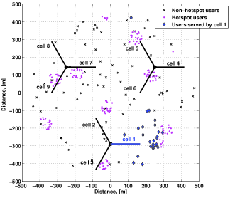
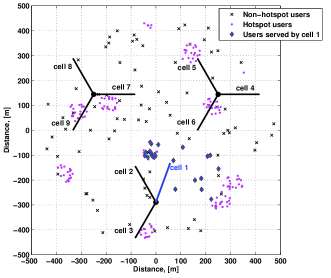
The network layout we have used is illustrated in Figure 2. Two layers of users are generated, with 30 users per macro cell area in total, out of which 2/3 (the dot markers) is in a randomly placed hotspot, and 1/3 (the x-markers) are distributed randomly and uniformly over the area. Each user equipment has an omni-directional antenna with 0 dBi antenna gain. The traffic demand corresponds to 400 kbit/s for all users within a duration of one second in the time domain.

Two network configurations are illustrated in Figure 2, with the only difference being the antenna direction of cell 1, which impacts the sets of users served by the cell and its neighbors. Intuitively, configuration two is inferior, since it results in that the hotspot users in cell 1’s original coverage area (see Figure 2(a)) is to be served by cell 8 and/or cell 9, although these users are relatively far away from the two cells. The likely impact is poorer link quality for the users in the handed-over hotspot as well as increased number of users to be served by the neighbors of cell 1. These effects are expected to be seen in the load of the neighbor cells.

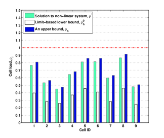
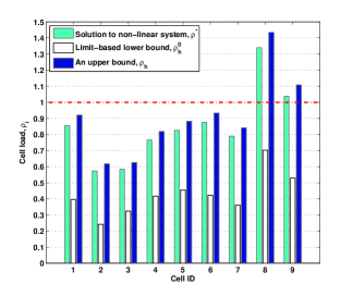
First, for both configurations, the existence of system solutions has been verified by finding $\boldsymbol{\rho}^{0}_{h}$ to the corresponding linear system, as described in Section V. Next, the non-linear coupling system (4) is solved using the non-linear optimization toolbox of MATLAB. Both $\boldsymbol{\rho}^{0}_{h}$ and $\boldsymbol{\rho}^{*}$ are shown in Figure 3. As expected, the load of cells 8 and 9 increases for the second configuration. At the same time, the load of cell 1 does not decrease either, even though it serves fewer users under the second configuration. This is due to a joint effect of several factors. Firstly, as can be seen from Figure 2(b), users served by cell 1 are likely to experience high interference from cell 6 and vice versa. From Figure 3(b), we observe that the load of cell 6 has also slightly increased. Secondly, the increased load in cells 8 and 9 implies more frequent transmissions in these cells and thus higher probability of interference to other cells; this in turn increases the load of the other cells, which can also be clearly seen in Figure 3. We further note that the solution $\boldsymbol{\rho}^{*}$ and thus the second configuration are not feasible from the capacity point of view.

In Figure 3, we also illustrate the load solutions to the linear systems described in Section VI, i.e., the upper bound $\boldsymbol{\rho}_{{\boldsymbol{\bar{h}}}}$ assuming $\boldsymbol{\widehat{\rho}}=\boldsymbol{\rho}^{0}_{{\boldsymbol{h}}}$. Table I provides further details of the quality of both the lower and upper bounds obtained for all 9 cells in Configuration 1 for which the solution is illustrated in Figure 2(a).

The tight upper bound indicates the efficiency of the linear approximation described in Section VI. In average, the estimation is deviates only a few percent from the true load value. For $\boldsymbol{\rho^{0}_{h}}$ the values are significantly lower than ${\boldsymbol{\rho}}^{*}$, as ${\boldsymbol{\rho}}={\boldsymbol{h}}^{0}({\boldsymbol{\rho}})$ represents a very optimistic view of load coupling. The observation sheds further light on the importance of fundamental characterization that the two systems are completely equivalent in solution existence, despite the large difference in numerical values of $\boldsymbol{\rho^{0}_{h}}$ and ${\boldsymbol{\rho}}^{*}$. Improving the lower bounds, although being beyond the scope of the current paper, is an interesting topic for future investigation. For example, in [35], the model discussed in this paper is applied for load balancing, for which very tight lower and upper bounds are obtained using few fixed-point iterations. It should be further noted that although the results have been presented for downlink, the model and the theoretical findings can be also applied to uplink.

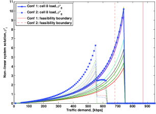
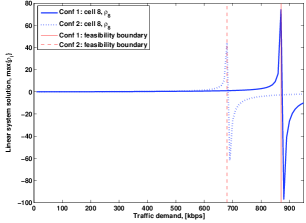
For the two network configurations, in Figure 4 we illustrate the behavior of the cell-load coupling with respect to demand, which is successively scaled up uniformly over the service area. Figure 4(a) and Figure 4(b) show, respectively, the results for the nonlinear load-coupling system (4), and the linear equation system ${\boldsymbol{\rho}}={\boldsymbol{h}}^{0}({\boldsymbol{\rho}})$ that provides lower estimation and characterizes feasibility of (4). The two configurations are distinguished by using respectively solid and dotted curves for the load solutions of nine cells. In Figure 4(a), the thicker curves represent the load of cell 8. For the linear system, only the maximum value among the cells is shown in Figure 4(b) for the sake of clarity.

From Figure 4(a), it is apparent that the solution values of (4) grow rapidly in the high-demand region, and becomes infeasible beyond some point. The feasibility boundaries for the two configurations are shown by the vertical lines. Configuration one is clearly superior, as its load values, shown by the solid curves, are below those of configuration two, and the feasibility boundary is considerably higher. For configuration two, cell 8 has the highest load (the dotted thick line). Using configuration one, some of the users are served by cell 1 instead (see Figure 2), leading to lower load in cell 8 (the solid thick line). Note that, for both configurations, when getting somewhat close to the infeasible region, the solver gives solutions containing some zero elements, indicating the solution is invalid (the system becomes unstable), before all the values abruptly drop to zeros showing infeasibility. When this occurs, the distance to the feasibility boundary is, in fact, significant. The behavior shows the importance of our analysis of characterizing feasibility exactly by the linear system ${\boldsymbol{\rho}}={\boldsymbol{h}}^{0}({\boldsymbol{\rho}})$.

In Figure 4(b), the linear system gives values growing consistently in demand. The system gives the feasibility boundary point of the non-linear load coupling equations, when the determinant of ${\boldsymbol{I}}-{\boldsymbol{H}}$, where $\boldsymbol{I}$ is the identity matrix and $\boldsymbol{H}$ is the matrix defined for ${\boldsymbol{h}}^{0}$, equals zero. After passing the boundary point, the linear system returns negative (infeasible) solutions. Hence the numerical results verify that the significance of the linear system to identifying solution existence. Moreover, using the linear system, one is able to conclude, as shown in Figure 4, that configuration one is clearly superior to configuration two.

VIII Conclusions

We have provided a theoretical analysis of the LTE load coupling system originally presented in [32] and have derived its fundamental properties, including concavity, behavior in limit, and solution uniqueness. We have also formulated the necessary and sufficient condition for solution existence, The analysis leads to a simple means for determining feasibility. In addition, we have presented two linear approximations. The analysis has been supported by theoretical proofs and numerical experiments and can serve as a fundamental basis for developing radio network planning and optimization strategies for LTE. Furthermore, the presented linearizations and the bounding-based optimization can potentially be used for more general convex optimization problems with similar properties.

(a) Feasible solution within network capacity: $0\leq{\boldsymbol{\rho}}\leq{1}$.

(b) Feasible solution beyond network capacity: $\exists{(i\in{\mathcal{N}})}|\rho_{i}>1$.

(c) Infeasible system: $S_{{\boldsymbol{\rho}}={\boldsymbol{f}}({\boldsymbol{\rho}})}=\emptyset$

Figure 1: An illustration of the load-coupling system of two cells.

(a) Configuration 1.

(b) Configuration 2.

Figure 2: Network configurations for numerical studies.

(a) Configuration 1: Feasible solution within network capacity.

(b) Configuration 2: Feasible solution beyond network capacity.

Figure 3: Load solutions for the two example network configurations.

TABLE I: Lower and upper bounds quality for Configuration 1

Bound	Cell 1	Cell 2	Cell 3	Cell 4	Cell 5	Cell 6	Cell 7	Cell 8	Cell 9
Upper bound, $\frac{|\boldsymbol{\rho^{0}_{h}}-\boldsymbol{\rho^{*}}|}{\boldsymbol{\rho^{*}}}\cdot{100\%}$	5.19	5.55	6.66	4.61	4.93	4.94	3.33	5.20	4.17
Lower bound, $\frac{|\boldsymbol{\rho_{\bar{h}}}-\boldsymbol{\rho^{*}}|}{\boldsymbol{\rho^{*}}}\cdot{100\%}$	48.05	48.15	44.44	43.08	43.21	50.62	51.66	46.82	50.00

(a) Growth of cell load with respect to demand for the load coupling system (4).

(b) Growth of cell load with respect to demand for the linear system ${\boldsymbol{\rho}}={\boldsymbol{h}}^{0}({\boldsymbol{\rho}})$.

Figure 4: System solution with respect to traffic demand.

References

- [1] 3GPP TS 36.814. Evolved Universal Terrestrial Radio Access (E-UTRA); Further advancements for E-UTRA physical layer aspects, v.9.0.0. http://www.3gpp.org
- [2] J. M. Aein. Power balancing in systems employing frequency reuse. COMSAT Technical Review, 3(2):277–300, 1973.
- [3] E. Amaldi, A. Capone, and F. Malucelli. Planning UMTS base station location: optimization models with power control and algorithms. IEEE Transactions on Wireless Communications, 2:939–952, 2003.
- [4] E. Amaldi, A. Capone, and F. Malucelli. Radio planning and coverage optimization of 3G cellular networks. Wireless Networks, 14:435–447, 2008.
- [5] E. Amaldi, A. Capone, F. Malucelli, and C. Mannino. Optimization problems and models for planning cellular networks. In M. Resende and P. Pardalos, editors, Handbook of Optimization in Telecommunications. Springer Science, 2006.
- [6] M. Assaad and A. Mourad. New frequency-time scheduling algorithms for 3GPP/LTE-like OFDMA air interface in the downlink. Proc. of IEEE VTC Spring ’08, 2008.
- [7] H. Boche, S. Naik, and T. Alpcan. Characterization of convex and concave resource allocation problems in interference coupled wireless systems. IEEE Transactions on Signal Processing, 59:2382–2394, May. 2011.
- [8] H. Boche, S. Naik, and M Schubert. Combinatorial characterization of interference coupling in wireless systems. IEEE Transactions on Signal Processing, 59:1697–1706, Jun. 2011.
- [9] H. Boche, S. Naik, and M Schubert. Pareto boundary of utility sets for multiuser wireless systems. IEEE Transactions on Networking, 19:589–602, Apr. 2011.
- [10] H. Boche and M. Schubert. Multiuser interference balancing for general interference functions – a convergence analysis. Proc. of IEEE ICC ’07, 2007.
- [11] H. Boche and S. Stańczak. Strict convexity of the feasible log-SIR region. IEEE Transactions on Communications, 56:1511–1518, Sep. 2008.
- [12] D. Catrein, L. A. Imhof, and R. Mathar. Power control, capacity, and duality of uplink and downlink in cellular CDMA systems. IEEE Transactions on Communications, 52:1777–1785, Oct. 2004.
- [13] E. Dahlman, S. Parkvall, J. Sköld 4G: LTE/LTE-Advanced for Mobile Broadband. Elsevier Science & Technology, 2011.
- [14] A. Eisenblätter and H.-F. Geerdes. Capacity optimization for UMTS: bounds and benchmarks for interference reduction. Proc. of IEEE PIMRC ’08, 2008.
- [15] A. Eisenblätter, H.-F. Geerdes, T. Koch, A. Martin, and R. Wessäly. UMTS radio network evaluation and optimization beyond snapshots. Mathematical Methods of Operations Research, 63:1–29, 2005.
- [16] A. Eisenblätter, T. Koch, A. Martin, T. Achterberg, A. Fügenschuh, A. Koster, O. Wegel, and R. Wessäly. Modelling feasible network configurations for UMTS. In: G. Anandalingam, and S. Raghavan, editors, Telecommunications Network Design and Management. Kluwer Academic Publishers, 2002.
- [17] H. Ekström. QoS control in the 3GPP evolved packet system. IEEE Communications Magazine, 76–83, February 2009.
- [18] M. Garcia-Lozano, S. Ruiz, and J. J. Olmos. UMTS optimum cell load balancing for inhomogeneous traffic patterns. Proc. of IEEE VTC Fall ’04, 2004.
- [19] S. A. Grandhi, R. Vijayan, and D. J. Goodman. Distributed algorithm for power control in cellular radio systems. Proc. of 30th Allerton Conf. on Communication, Control, and Computing, Sep. 1992.
- [20] J. Jan and K. B. Lee. Transmit power adaptation for multiuser OFDM systems. IEEE Journal on Selected Areas in Communications, 21:171–178, 2003.
- [21] S.-B. Lee, I. Pefkianakis, A. Meyerson, S. Xu, and S. Lu. Proportional fair frequency-domain packet scheduling for 3GPP LTE uplink. Proc. of IEEE INFOCOM ’09, pp. 2611–2615, 2009.
- [22] H. Lei, C. Fan, X. Zhang, and D. Yang. QoS aware packet scheduling algorithm for OFDMA systems. Proc. of IEEE VTC Fall ’07, 2007.
- [23] K. Majewski and M. Koonert. Conservative cell load approximation for radio networks with Shannon channels and its application to LTE network planning. Proc. of the 5th Advanced International Conference on Telecommunications, 2010.
- [24] K. Majewski, U. Türke, X. Huang, and B. Bonk. Analytical cell load assessment in OFDM radio networks. Proc. of IEEE PIMRC ’07, 2007.
- [25] R. Mathar and M. Schmeink. Optimal base station positioning and channel assignment for 3G mobile networks by integer programming. Annals of Operations Research, 107:225–236, 2001.
- [26] L. Mendo and J. M. Hernando. On dimension reduction for the power control problem. IEEE Transactions on Communications, 49(2):243–248, Feb. 2001.
- [27] P. Mogensen, W. Na, I. Z. Kovács, F. Frederiksen, A. Pokhariyal, K. I. Pedersen, T. Kolding, K. Hugl, and M. Kuusela. LTE capacity compared to the Shannon bound. Proc. of IEEE VTC Spring ’07, 2007.
- [28] M. Nawrocki, H. Aghvami, and M. Dohler. Understanding UMTS Radio Network Modelling, Planning and Automated Optimisation: Theory and Practice. Wiley, 2006.
- [29] J. Park, S. Hwang, and H.-S. Cho. A packet scheduling scheme to support real-time traffic in OFDMA systems. Proc. of IEEE VTC Spring ’07, 2007.
- [30] A. Pokhariyal, T. E. Kolding, and P. E. Mogensen. Performance of downlink frequency domain packet scheduling for the UTRAN long term evolution. Proc. of IEEE PIMRC ’06, 2006.
- [31] Z. Shen, J. G. Andrews, and B. L. Evans. Adaptive resource allocation in multiuser OFDM systems with proportional rate constraints. IEEE Transactions on Wireless Communications, 4:2726–2737, 2005.
- [32] I. Siomina, A. Furuskär, and G. Fodor. A mathematical framework for statistical QoS and capacity studies in OFDM networks. Proc. of IEEE PIMRC ’09, 2009.
- [33] I. Siomina, P. Värbrand, and D. Yuan. Automated optimization of service coverage and base station antenna configuration in UMTS networks. IEEE Wireless Communications Magazine, 13:16–25, 2006.
- [34] I. Siomina and D. Yuan. Optimization of pilot power for load balancing in WCDMA networks. Proc. of IEEE GLOBECOM ’04, 2004.
- [35] I. Siomina and D. Yuan. Load balancing in heterogeneous LTE: Range optimization via cell offset and load-coupling characterization. To appear in Proc. of IEEE ICC ’12, June 2012.
- [36] L. Song and J. Shen, editors. Evolved Cellular network Planning and Optimization for UMTS and LTE. CRC Press, 2010.
- [37] S. Stańczak, M. Wiczanowski, and H. Boche. Distributed utility-based power control: objectives and algorithms. IEEE Transactions on Signal Processing, 55:4053–4068, Oct. 2007.
- [38] S. Stańczak, A. Feistel, M. Wiczanowski, and H. Boche. Utility-based power control with QoS support. Wireless Networks, 16:1691–1705, 2010.
- [39] M. Wiczanowski, H. Boche, and S. Stańczak. An algorithm for optimal resource allocation in cellular networks with elastic traffic. IEEE Transactions on Communications, 57:41–44, Jan. 2009.
- [40] M. Wiczanowski, S. Stańczak, and H. Boche. Providing quadratic convergence of decentralized power control in wireless networks – the method of min-max functions. IEEE Transactions on Signal Processing, 56:4053–4068, Aug. 2008.
- [41] J. Zander. Performance of optimum transmitter power control in cellular radio systems. IEEE Transactions on Vehicular Technology, 41:57–62, Feb. 1992.
- [42] J. Zander. Distributed co-channel interference control in cellular radio systems. IEEE Transactions on Vehicular Technology., 41:305–311, Aug. 1992.
- [43] J. Zhang, J. Yang, M. E. Aydin, and J. Y. Wu. UMTS base station location planning: a mathematical model and heuristic optimisation algorithms. IET Communications 1:1007–1014, 2007.
- [44] I. Zhao, M. Joonert, A. Timm-Giel, and C. Görg. Highly efficient simulation approach for the network planning of HSUPA in UMTS. Proc. of IEEE VTC Spring ’08, 2008.