Convolutive decomposition and fast summation methods for discrete-velocity approximations of the Boltzmann equation

Abstract.

Discrete-velocity approximations represent a popular way for computing the Boltzmann collision operator. The direct numerical evaluation of such methods involve a prohibitive cost, typically $O(N^{2d+1})$ where $d$ is the dimension of the velocity space. In this paper, following the ideas introduced in [27, 28], we derive fast summation techniques for the evaluation of discrete-velocity schemes which permits to reduce the computational cost from $O(N^{2d+1})$ to $O(\bar{N}^{d}N^{d}\log_{2}N)$, $\bar{N}\ll N$, with almost no loss of accuracy.

Keywords. Boltzmann equation; Discrete-velocity approximations; Discrete-Velocity Methods; Fast summation methods; Farey series; Convolutive decomposition.

AMS Subject Classifications. 65T50, 68Q25, 74S25, 76P05

1. Introduction

Among deterministic methods to approximate the Boltzmann collision integral, one of the most popular is represented by discrete velocity models (DVM). These methods [7, 25, 3, 14, 30, 36, 26, 6] are based on a regular grid in the velocity field and construct a discrete collision mechanics on the points of the quadrature rule in order to preserve the main physical properties.

As compared to Monte-Carlo methods, these methods have certain number of assets: accuracy, absence of statistical fluctuations, and the fact that the distribution function is explicitly represented in the velocity space. However their computational cost is more than quadratic and they cannot compete with the linear cost of a Monte Carlo approach. Indeed the “naive” cost of a product quadrature formula for the $(d-1)+d$ fold Boltzmann collision integral in dimension $d$ is $O(M^{d-1}N^{d})$, where $M$ is related to the angle and $N$ to the velocity discretizations. More concretely Buet presented in [7] a DVM algorithm widely used since then in $O(N^{2d+1+\varepsilon})$ for all $\varepsilon>0$ (and a constant depending on $\varepsilon$); Michel and Schneider algorithm in [26] is $O(N^{2d+\delta})$ where $\delta$ depends on $d$ and is close to $1$; finally the method of Panferov and Heinz [30] is $O(N^{2d+1})$. For this reason several acceleration techniques for DVM have been proposed in the past literature. We do not seek to review them here, and refer the reader to [7, 22, 24, 35, 37].

More recently a new class of methods based on the use of spectral techniques in the velocity space has attracted the attention of the scientific community. The method first developed for the Boltzmann equation in [31] is based on a Fourier-Galerkin approximation of the integral collision operator. As shown in [32, 33] the method permits to obtain spectrally accurate solution at a reduced computational cost of $O(N^{2d})$. A proof of stability and convergence for this method has been given in [16]. Finally the method has been extended to the case of the quantum Boltzmann collision operator [15, 20]. Other methods based on spectral techniques have been developed in [4, 18].

One of the major differences between DVM and spectral methods is that in the latter the interaction kernel of the Boltzmann collision integral is not modified in order to obtain a conservative equation on a bounded domain. This aspect has a profound influence on the resulting structure of the algorithm since most of the symmetries which are present in the original operator are preserved. Using this fact, in [27, 28], the authors developed a numerical technique based on the Fast Fourier Transform (FFT) that permits to reduce the cost of spectral method from $O(N^{2d})$ to $O(M^{d-1}N^{d}\log_{2}N)$ where $M$ is the number of angle discretizations. These ideas have been successfully used in [17] to compute space non homogeneous solutions of the Boltzmann equation.

In this paper we will consider general discrete velocity approximation of the Boltzmann equation without any modification to the original collision kernel and show how the FFT techniques developed in [27, 28] can be adapted to this case to obtain acceleration algorithms. In this way, for a particular class interactions using a Carleman-like representation of the collision operator we are able to derive discrete velocity approximations that can be evaluated through fast algorithms at a cost of $O(\bar{N}^{d}N^{d}\log_{2}N)$, $\bar{N}\ll N$. The class of interactions includes Maxwellian molecules in dimension two and hard spheres molecules in dimension three.

Let us emphasize here that a detailed analysis of the computational complexity in DVM is non trivial since imposing conservations on the points of the quadrature rule originates a summation formula that requires the exact enumeration of the set of involved orthogonal directions in $\mathbb{Z}^{d}$.

The rest of the paper is organized in the following way. In the next Section we introduce briefly the Boltzmann equation and give a Carleman-like representation of the collision operator which is used as a starting point for the development of our methods. In Section 3 a fast DVM method is introduced together with a detailed analysis of its computational complexity. In Section 4, we present some numerical results obtained with the fast and the classical DVM methods.

2. Preliminaries

2.1. The Boltzmann equation

The Boltzmann equation describes the behavior of a dilute gas of particles when the only interactions taken into account are binary elastic collisions. It reads for $x,v\in\mathbb{R}^{d}$ ($d\geq 2$)

$$\frac{\partial f}{\partial t}+v\cdot\nabla_{x}f=Q(f,f)$$

where $f(t,x,v)$ is the time-dependent particle distribution function in the phase space. The Boltzmann collision operator $Q$ is a quadratic operator local in $(t,x)$. The time and position acts only as parameters in $Q$ and therefore will be omitted in its description

(2.1) $$Q(f,f)(v)=\int_{v_{*}\in\mathbb{R}^{d}}\int_{\sigma\in\mathbb{S}^{d-1}}B(\cos\theta,|v-v_{*}|)\,\left[f^{\prime}_{*}f^{\prime}-f_{*}f\right]\,d\sigma\,dv_{*}.$$

In (2.1) we used the shorthand $f=f(v)$, $f_{*}=f(v_{*})$, $f^{{}^{\prime}}=f(v^{\prime})$, $f_{*}^{{}^{\prime}}=f(v_{*}^{{}^{\prime}})$. The velocities of the colliding pairs $(v,v_{*})$ and $(v^{\prime},v^{\prime}_{*})$ are related by

$$v^{\prime}=\frac{v+v_{*}}{2}+\frac{|v-v_{*}|}{2}\sigma,\qquad v^{\prime}_{*}=\frac{v+v^{*}}{2}-\frac{|v-v_{*}|}{2}\sigma.$$

The collision kernel $B$ is a non-negative function which by physical arguments of invariance only depends on $|v-v_{*}|$ and $\cos\theta={\widehat{g}}\cdot\sigma$ (where ${\widehat{g}}=(v-v_{*})/|v-v_{*}|$).

Boltzmann’s collision operator has the fundamental properties of conserving mass, momentum and energy

$$\int_{v\in{\mathbb{R}}^{d}}Q(f,f)\phi(v)\,dv=0,\qquad\phi(v)=1,v,|v|^{2}$$

and satisfies the well-known Boltzmann’s $H$-theorem

$$-\frac{d}{dt}\int_{v\in{\mathbb{R}}^{d}}f\log f\,dv=-\int_{v\in{\mathbb{R}}^{d}}Q(f,f)\log(f)\,dv\geq 0.$$

The functional $-\int f\log f$ is the entropy of the solution. Boltzmann $H$-theorem implies that any equilibrium distribution function, i.e. any function which is a maximum of the entropy, has the form of a locally Maxwellian distribution

$$M(\rho,u,T)(v)=\frac{\rho}{(2\pi T)^{d/2}}\exp\left(-\frac{|u-v|^{2}}{2T}\right),$$

where $\rho,\,u,\,T$ are the density, mean velocity and temperature of the gas

$$\rho=\int_{v\in{\mathbb{R}}^{d}}f(v)dv,\quad u=\frac{1}{\rho}\int_{v\in{\mathbb{R}}^{d}}vf(v)dv,\quad T=\frac{1}{d\rho}\int_{v\in{\mathbb{R}}^{d}}|u-v|^{2}f(v)dv.$$

For further details on the physical background and derivation of the Boltzmann equation we refer to [12] and [38].

2.2. Carleman-like representation in bounded domains

In this short paragraph we shall approximate the collision operator on a bounded domain starting from a representation which somehow conserves more symmetries of the collision operator when one truncates it in a bounded domain. This representation was used in [1, 4, 5, 21, 28] and is close to the classical Carleman representation (cf. [10]).

The starting point of this representation is the identity

(2.2) $$\frac{1}{2}\,\int_{\mathbb{S}^{d-1}}F(|u|\sigma-u)\,d\sigma=\frac{1}{|u|^{d-2}}\,\int_{\mathbb{R}^{d}}\delta(2\,x\cdot u+|x|^{2})\,F(x)\,dx.$$

It can be verified easily by completing the square in the delta Dirac function, taking the spherical coordinate $x=r\,\sigma$ and performing the change of variable $r^{2}=s$. Then, setting $u=v-v_{*}$ and $r=|u|$, we have the following Lemma.

Lemma 2.1 (Cf. [28], subsection 2.1).

Introducing the change of variables

$$x=\frac{1}{2}\,r\,\sigma,\quad y=v_{*}-v-x,$$

the collision operator (2.1) can be rewritten in the form

$$Q(f,f)(v)=\int_{x\in\mathbb{R}^{d}}\int_{y\in\mathbb{R}^{d}}\tilde{B}(x,y)\,\delta(x\cdot y)\left[f(v+y)\,f(v+x)-f(v+x+y)\,f(v)\right]\,dx\,dy,$$

where

(2.3) $$\tilde{B}(x,y)=\tilde{B}(|x|,|y|)=2^{d-1}\,B\left(\frac{|x|}{\sqrt{|x|^{2}+|y|^{2}}},\sqrt{|x|^{2}+|y|^{2}}\right)\,(|x|^{2}+|y|^{2})^{-\frac{d-2}{2}}.$$

Now let us consider the bounded domain $\mathcal{D}_{T}=[-T,T]^{d}$ ($0<T<+\infty$). First one can remove the collisions connecting with some points out of the box. This is the natural preliminary stage for deriving conservative schemes based on the discretization of the velocity. In this case there is no need for a truncation on the modulus of $x$ and $y$ since we impose them to stay in the box. It yields

$$Q^{\mbox{tr}}(f,f)(v)=\int\int_{\big{\{}x,\,y\,\in\,\mathbb{R}^{d}\ |\ v+x,\,v+y,\,v+x+y\,\in\,\mathcal{D}_{T}\big{\}}}\tilde{B}(x,y)\,\delta(x\cdot y)\\ \left[f(v+y)\,f(v+x)-f(v+x+y)\,f(v)\right]\,dx\,dy$$

defined for $v\in\mathcal{D}_{T}$. One can easily check that the following weak form is satisfied by this operator

(2.4) $$\int Q^{\mbox{tr}}(f,f)\,\varphi(v)\,dv=\frac{1}{4}\,\int\int\int_{\big{\{}v,\,x,\,y\,\in\,\mathbb{R}^{d}\ |\ v,\,v+x,\,v+y,\,v+x+y\,\in\,\mathcal{D}_{T}\big{\}}}\tilde{B}(x,y)\,\delta(x\cdot y)\\ f(v+x+y)\,f(v)\left[\varphi(v+y)+\varphi(v+x)-\varphi(v+x+y)-\varphi(v)\right]\,dv\,dx\,dy$$

and this implies conservation of mass, momentum and energy as well as the $H$-theorem on the entropy. The problem of this truncation on a bounded domain is the fact that we have changed the collision kernel itself by adding some artificial dependence on $v,v_{*},v^{\prime},v^{\prime}_{*}$. In this way convolution-like properties are broken.

A different approach consists in truncating the integration in $x$ and $y$ by setting them to vary in $\mathcal{B}_{R}$, the ball of center $0$ and radius $R$. For a compactly supported function $f$ with support $\mathcal{B}_{S}$, we take $R=S$ in order to obtain all possible collisions. Since we aim at using the FFT algorithm to evaluate the resulting quadrature approximation, and hence we will make use of periodic distribution functions, we must take into account the aliasing effect due to periods superposition in the Fourier space. As for the spectral method a geometrical argument (see [32] for further details) shows that using the periodicity of the function it is enough to take $T\geq(3+\sqrt{2})S/2$ to prevent intersections of the regions where $f$ is different from zero.

The operator now reads

(2.5) $$Q^{R}(f,f)(v)=\int_{x\in\mathcal{B}_{R}}\int_{y\in\mathcal{B}_{R}}\tilde{B}(x,y)\,\delta(x\cdot y)\\ \left[f(v+y)f(v+x)-f(v+x+y)f(v)\right]\,dx\,dy$$

for $v\in\mathcal{D}_{T}$. The interest of this representation is to preserve the real collision kernel and its properties. It is easy to check that, except for the aliasing effect, the operator preserves all the original conservation properties, see the weak form in equation (2.6).

In order to understand the possible effect of periods superposition we can rely on the following weak form valid for any function $\varphi$ periodic on $\mathcal{D}_{T}$

(2.6) $$\int_{\mathcal{D}_{T}}Q^{R}(f,f)\,\varphi(v)\,dv=\frac{1}{4}\,\int_{v\in\mathcal{D}_{T}}\int_{x\in\mathcal{B}_{R}}\int_{y\in\mathcal{B}_{R}}\tilde{B}(x,y)\,\delta(x\cdot y)\\ f(v+x+y)f(v)\left[\varphi(v+y)+\varphi(v+x)-\varphi(v+x+y)-\varphi(v)\right]\,dv\,dx\,dy.$$

About the conservation properties one can show that

1. The only invariant $\varphi$ is $1$: it is the only periodic function on $\mathcal{D}_{T}$ such that

   $$\varphi(v+y)+\varphi(v+x)-\varphi(v+x+y)-\varphi(v)=0$$

   for any $v\in\mathcal{D}_{T}$ and $x\bot y\in\mathcal{B}_{R}$ (see [11] for instance). It means that the mass is locally conserved but not necessarily the momentum and energy.

2. When $f$ is even there is global conservation of momentum, which is $0$ in this case. Indeed $Q^{R}$ preserves the parity property of the solution, which can be checked using the change of variable $x\to-x$, $y\to-y$.

3. The collision operator satisfies formally the $H$-theorem

   $$\int_{v\in{\mathbb{R}}^{d}}Q^{R}(f,f)\log(f)\,dv\leq 0.$$

4. If $f$ has compact support included in $\mathcal{B}_{S}$ with $T\geq(3+\sqrt{2})S/2$ (no-aliasing condition, see [32] for a detailed discussion) and $R=S$, then no unphysical collisions occur and thus mass, momentum and energy are preserved. Obviously this compactness is not preserved with time since the collision operator spreads the support of $f$ by a factor $\sqrt{2}$.

2.3. Application to discrete-velocity models

The representation $Q^{R}$ of this section can also be used to derive discrete velocity models (DVM). Any DVM can be written in the general form

(2.7) $$D_{i}(f,f)=\sum_{j,k,l\,\in\,\mathbb{Z}^{d}}\Gamma_{i,j}^{k,l}\big{[}f_{k}f_{l}-f_{i}f_{j}\big{]},$$

where $D_{i}$ denotes the discrete Boltzmann collision operator and the integer indexes refer to the points in the computational grid.

In order to keep conservations the coefficients $\Gamma_{i,j}^{k,l}$ are defined by

(2.8) $$\Gamma_{i,j}^{k,l}={\bf 1}(i+j-k-l)\,{\bf 1}(|i|^{2}+|j|^{2}-|k|^{2}-|l|^{2})\,B(|k-i|,|l-j|)\,w_{i,j}^{k,l}$$

where ${\bf 1}$ denotes the function on $\mathbb{Z}$ defined by ${\bf 1}(z)=1$ if $z=0$ and $0$ elsewhere, and $w_{i,j}^{k,l}>0$ are the weights of the quadrature formula, which characterize the different DVM. The function $B>0$ is the discrete collision kernel. One can check on this formulation that the scheme satisfies the usual conservation laws and entropy inequality (see [34, 8] and the references therein). More details on the DVM schemes can also be found in [8].

Thanks to equations (2.7) and (2.8), we can write at the discrete level the same representation as in the continuous case

$$D_{i}(f,f)=\sum_{k,l\,\in\,\mathbb{Z}^{d}}\widetilde{\Gamma}_{k,l}\big{[}f_{i+k}f_{i+l}-f_{i}f_{i+k+l}\big{]}$$

with

$$\widetilde{\Gamma}_{k,l}=2^{d-1}\,B\left(\frac{|k|}{\sqrt{|k|^{2}+|l|^{2}}},\sqrt{|k|^{2}+|l|^{2}}\right)\,(|k|^{2}+|l|^{2})^{-\frac{d-2}{2}}{\bf 1}(k\cdot l)\,w_{k,l}.$$

This is coherent with the DVM obtained by quadrature starting from the Carleman representation in [30].

Now again when one is interested to compute the DVM in a bounded domain there are two possibilities. First as in the case of $Q^{\mbox{tr}}$ one can force the discrete velocities to stay in a box, which yields for $i\in\llbracket-N,N\rrbracket^{d}$ (again using the one index notation for $d$-dimensional sums)

$$D^{\mbox{tr}}_{i}(f,f)=\sum_{\begin{subarray}{c}k,l\\ -N\leq\,i+k,\,i+l,\,i+k+l\leq N\end{subarray}}\widetilde{\Gamma}_{k,l}\big{[}f_{i+k}f_{i+l}-f_{i}f_{i+k+l}\big{]}.$$

This new discrete operator is completely conservative but the collision kernel is not invariant anymore according to $i$, which breaks the convolution properties and then prevents the derivation of a fast algorithm.

The other possibility is to periodize the function $f$ over the box and truncate the sum in $k$ and $l$. It yields for a given truncation parameter $\tilde{N}\in\mathbb{N}^{*}$

(2.9) $$D^{\tilde{N}}_{i}(f,f)=\sum_{-\tilde{N}\leq k,l\leq\tilde{N}}\widetilde{\Gamma}_{k,l}\big{[}f_{i+k}f_{i+l}-f_{i}f_{i+k+l}\big{]},$$

for any $i\in\llbracket-N,N\rrbracket^{d}$.

It is easy to see that $D^{\tilde{N}}$ satisfies exactly a discrete weak form and conservation properties similar to $Q^{R}$. Let us briefly state and sketch the proof of the conservation and stability properties of the scheme.

Proposition 2.2.

Assume that the quadrature weight $w_{i,j}^{k,l}>0$ are positive. Consider some truncation numbers $\tilde{N}\leq N\in\mathbb{N}^{*}$ and some non-negative initial data $f_{i}(0)\geq 0$, $i\in\llbracket-N,N\rrbracket^{d}$. Then the discrete evolution equation

$$\partial_{t}f_{i}=D^{\tilde{N}}_{i}(f,f)=\sum_{-\tilde{N}\leq k,l\leq\tilde{N}}\widetilde{\Gamma}_{k,l}\big{[}f_{i+k}f_{i+l}-f_{i}f_{i+k+l}\big{]},\qquad i\in\llbracket-N,N\rrbracket^{d},$$

is globally well-posed in $\mathbb{R}^{\llbracket-N,N\rrbracket^{d}}$. Moreover the coefficients $f_{i}(t)$ are non-negative for all time, and

$$\forall\,t\geq 0,\quad\sum_{i\in\llbracket-N,N\rrbracket^{d}}f_{i}(t)=\sum_{i\in\llbracket-N,N\rrbracket^{d}}f_{i}(0).$$

Remark 2.3.

The DVM scheme we consider therefore preserves non-negativity, but let us also emphasize that it preserves momentum and energy up to aliasing issues. This is different from spectral methods where the truncation of Fourier modes introduces an additional error in the conservation laws. Concerning the spectral method, stability and convergence have been proved recently in [17] to hold in $L^{1}$ but only asymptotically, i.e. for $N$ big enough related to the initial data.

Proof of Proposition 2.2.

We have the following $L^{1}$-like estimate

$$\frac{d}{dt}\sum_{i\in\llbracket-N,N\rrbracket^{d}}\left|f_{i}(t)\right| =\sum_{i\in\llbracket-N,N\rrbracket^{d}}\left|\sum_{-\tilde{N}\leq k,l\leq\tilde{N}}\widetilde{\Gamma}_{k,l}\big{[}f_{i+k}f_{i+l}-f_{i}f_{i+k+l}\big{]}\right|$$

(2.10) $$\leq C\,\left(\sum_{i\in\llbracket-N,N\rrbracket^{d}}|f_{i}|\right)^{2}.$$

The use of a Grönwall argument then gives the local well-posedness of the scheme in $\mathbb{R}^{\llbracket-N,N\rrbracket^{d}}$. Moreover, given a local solution $f_{i}(t)$, for $t\in[0,T]$ and $T>0$, it is clear by construction that the conservation of mass holds.

The proof of preservation of non-negativity for this solution is essentially contained in the pioneering work of Carleman [10]. We will sketch its proof in the following. Let us rewrite the system of ordinary differential equations satisfied by $f_{i}$ for a fixed $i\in\llbracket-N,N\rrbracket^{d}$ as

(2.11) $$\frac{d}{dt}f_{i}+f_{i}\sum_{-\tilde{N}\leq k,l\leq\tilde{N}}f_{i+k+l}=\sum_{-\tilde{N}\leq k,l\leq\tilde{N}}\widetilde{\Gamma}_{k,l}\,f_{i+k}\,f_{i+l}.$$

Let us assume by contradiction that we have

$$\left\{\begin{aligned} &f_{j}\,(t)>0,\quad\forall t\in[0,T[,\quad\forall j\in\llbracket-N,N\rrbracket^{d},\\ &~{}\\ &f_{i}\,(T)=0.\end{aligned}\right.$$

Then, we have necessarily

$$f_{i}^{\prime}\,(T)\leq 0,$$

and thus, according to (2.11),

$$\sum_{-\tilde{N}\leq k,l\leq\tilde{N}}\widetilde{\Gamma}_{k,l}\,f_{i+k}(T)\,f_{i+l}(T)\leq 0.$$

By continuity in time of $f_{j}$, it comes that

$$f_{j}(T)=0,\quad\forall j\in\llbracket-N,N\rrbracket^{d}.$$

As these conditions implies using (2.11) that $f_{j}(t)=0$ for all $t\in[0,T]$, we have a contradiction with the non-negativity of the initial condition.

Finally, the conservations of mass and non-negativity implies the preservation of $L^{1}$ norm, and we can iterate the argument giving the local well-posedness (still using inequality (2.10)) to obtain the global well-posedness of the scheme.

∎

Finally one can derive the following consistency result from [30, Theorem 3] in the case of hard spheres collision kernel with $d=3$

Theorem 2.4.

Assume that $f,g\in C^{k}(\mathbb{R}^{3})$ ($k\geq 1$) with compact support $\mathcal{B}_{S}$. The uniform grid of step $h$ is constructed on the box $\,\mathcal{D}_{T}$ with the no-aliasing condition $T\geq(3+\sqrt{2})S/2$. Then for $\tilde{N}=[S/h]$ (where $[\,\cdot\,]$ denotes the floor function) and $h>0$ sufficiently small,

$$\left\|Q(g,f)-D^{\tilde{N}}_{\cdot}(g,f)\right\|_{L^{\infty}(\mathbb{Z}_{h})}\leq C\,h^{r}$$

where $D^{\tilde{N}}_{\cdot}$ is the DVM operator defined in (2.9) (for the precise quadrature weights derived in [30]) on the grid above-mentioned, and $f_{i}=f(ih)$. Here $r=k/(k+3)$ and the constant $C$ is independent on $h$.

Remark 2.5.

As can be seen from Theorem 2.4, the periodized DVM presented in this subsection is expected to have a quite poor accuracy. On the contrary the spectral method [31], even in the fast version of [28], has been proven to be spectrally accurate, i.e. of infinite order for smooth solutions. Nevertheless this periodized DVM has some interesting features compared to the spectral method: preservation of sign, stability, and preservation of the conservation laws up to aliasing issues.

3. Fast DVM’s algorithms

The fast algorithms developed for the spectral method in [28] can be in fact extended to the periodized DVM method. The method that originates was triggered by the reading of the direct FFT approach proposed in [1, 5, 4].

3.1. Principle of the method: a pseudo-spectral viewpoint

We start from the periodized DVM in $\llbracket-N,N\rrbracket^{d}$ with representation (2.9) and as in the continuous case we set, for $k,l\in-\tilde{N}\leq k,l\leq\tilde{N}$,

$$\tilde{B}(|k|,|l|)=2^{d-1}\,B\left(\frac{|k|}{\sqrt{|k|^{2}+|l|^{2}}},\sqrt{|k|^{2}+|l|^{2}}\right)\,(|k|^{2}+|l|^{2})^{-\frac{d-2}{2}}.$$

With this notation

$$\widetilde{\Gamma}_{k,l}={\bf 1}(k\cdot l)\,\tilde{B}(|k|,|l|)\,w_{k,l},$$

and thus the DVM becomes

$$\partial_{t}f_{i}=\sum_{-\tilde{N}\leq k,l\leq\tilde{N}}{\bf 1}(k\cdot l)\,\tilde{B}(|k|,|l|)\,w_{k,l}\,\big{[}f_{i+k}f_{i+l}-f_{i}f_{i+k+l}\big{]}.$$

Now we transform this set of ordinary differential equations into a new one using the involution transformation of the discrete Fourier transform on the vector $(f_{i})_{-N\leq i\leq N}$. This involution reads for $I\in\llbracket-N,N\rrbracket^{d}$

$$\tilde{f}_{I}=\frac{1}{2N+1}\,\sum_{i=-N}^{N}f_{i}\,{\bf e}_{-I}(i),\hskip 22.76228ptf_{i}=\sum_{I=-N}^{N}\tilde{f}_{I}\,e_{I}(i)$$

where ${\bf e}_{K}(k)$ denotes $e^{\frac{2i\pi\,K\cdot k}{2N+1}}$, and thus the set of differential equations becomes

$$\partial_{t}\tilde{f}_{I} = \sum_{K,L=-N}^{N}\left(\frac{1}{2N+1}\,\sum_{i=-N}^{N}{\bf e}_{K+L-I}(i)\right)\,$$

$$\left[\sum_{-\tilde{N}\leq k,l\leq\tilde{N}}{\bf 1}(k\cdot l)\,\tilde{B}(|k|,|l|)\,w_{k,l}\,\left({\bf e}_{K}(k){\bf e}_{L}(l)-{\bf e}_{L}(k+l)\right)\right]\,\tilde{f}_{K}\,\tilde{f}_{L}$$

for $-N\leq I\leq N$. We have the following identity

$$\frac{1}{2N+1}\,\sum_{i=-N}^{N}{\bf e}_{K+L-I}(i)={\bf 1}(K+L-I)$$

and so the set of equations is

(3.1) $$\partial_{t}\tilde{f}_{I}=\sum_{\begin{subarray}{c}K,L=-N\\ K+L=I\end{subarray}}^{N}\tilde{\beta}(K,L)\,\tilde{f}_{K}\,\tilde{f}_{L}$$

with

$$\tilde{\beta}(K,L)=\sum_{-\tilde{N}\leq k,l\leq\tilde{N}}{\bf 1}(k\cdot l)\,\tilde{B}(|k|,|l|)\,w_{k,l}\,\big{[}{\bf e}_{K}(k){\bf e}_{L}(l)-{\bf e}_{L}(k+l)\big{]}=\beta(K,L)-\beta(L,L)$$

where

(3.2) $$\beta(K,L)=\sum_{-\tilde{N}\leq k,l\leq\tilde{N}}{\bf 1}(k\cdot l)\,\tilde{B}(|k|,|l|)\,w_{k,l}\,{\bf e}_{K}(k){\bf e}_{L}(l).$$

Let us first remark that this new formulation allows to reduce the usual cost of computation of a DVM exactly to $O(N^{2d})$ (as with the usual spectral method) instead of $O(N^{2d+\delta})$ for $\delta\sim 1$ [7, 26, 30]. Note however that the $(2N+1)^{d}\times(2N+1)^{d}$ matrix of coefficients $(\beta(K,L))_{K,L}$ has to be computed and stored first, thus the storage requirements are larger with respect to usual DVM. Nevertheless symmetries in the matrix can substantially reduce this cost.

Now the aim is to give an expansion of $\beta(K,L)$ of the form

$$\beta_{K,L}\simeq\sum_{p=1}^{M}\alpha_{p}(K)\,\alpha^{\prime}_{p}(L),$$

for a parameter $M\in\mathbb{N}^{*}$ to be defined later. Indeed, this formulation will allow us to write (3.1) as a sum of $M$ discrete convolutions and then this algorithm can be computed in $O(M\,N^{d}\log_{2}(N))$ operations by using standard FFT techniques [13, 9], as in the fast spectral method.

3.2. Expansion of the discrete kernel modes

We make a decoupling assumption on the collision kernel as in the spectral case [28]

(3.3) $$\tilde{B}(|k|,|l|)\,w_{k,l}=a(k)\,b(l).$$

Note that the DVM constructed by quadrature in dimension $3$ for hard spheres in [30] on the cartesian velocity grid $h\,\mathbb{Z}^{3}$ (for $h>0$) satisfies this decoupling assumption with $a(k)=h^{5}\,|k|/\mbox{gcd}(k_{1},k_{2},k_{3})$ and $b(l)=1$ (see [30, Formula (20-21)]), and $\mbox{gcd}(k_{1},k_{2},k_{3})$ denotes the greater common divisor of the three integers. For Maxwell molecules in dimension $2$ on the grid $h\,\mathbb{Z}^{2}$, these coefficients are $a(k)=h^{3}\,|k|/\mbox{gcd}(k_{1},k_{2})$ and $b(l)=1$.

The difference here with the spectral method, which is a continuous numerical method, is that we have to enumerate the set of $\{-\tilde{N}\leq k,l\leq\tilde{N}\ |\ k\,\bot\,l\,\}$. This motivates for a detailed study of the number of lines passing through $0$ and another point in the grid (this is equivalent to the study of this set), in order to compute the complexity of the method in term of $N$.

To this purpose let us introduce the Farey series and a new parameter $0\leq\bar{N}\leq\tilde{N}$ for the size of the grid used to compute the number of directions. The usual Farey series is

$$\mathcal{F}_{\bar{N}}^{1}=\left\{(p,q)\in\llbracket 0,\bar{N}\rrbracket^{2}\ |\ 0\leq p\leq q\leq\bar{N},\ q\geq 1,\ \mbox{and}\ \mbox{gcd}(p,q)=1\right\}$$

where $\mbox{gcd}(p,q)$ denotes again the greater common divisor of the two integers (more details can be found in [19]). We gave a schematic representation of the two dimensional Farey series in Figure 1. It is straightforward to see that the number of lines $A_{\bar{N}}^{1}$ passing through $0$ in the grid $\llbracket-\bar{N},\bar{N}\rrbracket^{2}$ is

$$A_{\bar{N}}^{1}=4\left(\left|\mathcal{F}_{\bar{N}}^{1}\right|-1\right),$$

where the factor $4$ allows to take into account the permutations when counting the couples $(p,q)$ as well as the ordering (symmetries in Figure 1), minus the line which is repeated during the symmetry process.

Figure 1. Representation of the Farey series $\mathcal{F}_{\bar{N}}^{1}$ and of $\mathcal{A}_{\bar{N}}^{1}$, the primal representant of lines in $[-N,N]$ associated, for $N=7$ and $\bar{N}=3$

Similarly one can define the set

$$\mathcal{F}^{2}_{\bar{N}}=\left\{(p,q,r)\in\llbracket 0,\bar{N}\rrbracket^{3}\ |\ 0\leq p\leq q\leq r\leq\bar{N},\ r\geq 1,\ \mbox{and}\ \mbox{gcd}(p,q,r)=1\right\}$$

and the number of lines $A^{2}_{\bar{N}}$ passing through $0$ in the grid $\llbracket-\bar{N},\bar{N}\rrbracket^{3}$ is

$$A^{2}_{\bar{N}}=24\left(\left|\mathcal{F}^{2}_{\bar{N}}\right|-\left|\mathcal{F}^{1}_{\bar{N}}\right|\right)-2\,A^{1}_{\bar{N}}$$

all possible permutations of the three numbers times $4$ and minus the interfaces $2A^{1}_{\bar{N}}$ accounting for the possible negative values by symmetry, minus $24\left|\mathcal{F}^{1}_{\bar{N}}\right|$ for the spurious terms when two equal numbers are swapped. The exponents of the Farey series refer to the dimension of the space of lines (which is $d-1$). Now let us estimate the cardinals of $\mathcal{F}^{1}_{\bar{N}}$ and $\mathcal{F}^{2}_{\bar{N}}$.

Lemma 3.1.

The Farey series in dimension $d=2$ and $d=3$ satisfy the following asymptotic behavior

$$\left|\mathcal{F}^{1}_{\bar{N}}\right| = \frac{\bar{N}^{2}}{2\,\zeta(2)}+O(\bar{N}\,\log\bar{N})=\frac{3\bar{N}^{2}}{\pi^{2}}+O(\bar{N}\,\log\bar{N}),$$

$$\left|\mathcal{F}^{2}_{\bar{N}}\right| = \frac{\bar{N}^{3}}{{12}\,\zeta(3)}+O(\bar{N}^{2}),$$

where $\zeta(s)=\sum_{n\geq 0}n^{-s}$ denotes the usual Riemann zeta function.

Remark 3.2.

In dimension $d$, the formula would be

$$\mathcal{F}^{d-1}_{\bar{N}}=\Big{\{}(p_{1},p_{2},\dots,p_{d})\in\llbracket 0,\bar{N}\rrbracket^{d}\ |\,0\leq p_{1}\leq p_{2}\leq\dots\leq p_{d}\leq\bar{N},\ p_{d}\geq 1\\ \mbox{and gcd}(p_{1},p_{2},\dots,p_{d})=1\Big{\}}.$$

The cardinal of $\mathcal{F}^{d-1}_{\bar{N}}$ could be computed by induction with the same tools as in the proof:

$$\left|\mathcal{F}^{d-1}_{\bar{N}}\right|=C_{d}\,\frac{\bar{N}^{d}}{\zeta(d)}+O(\bar{N}^{d-1}).$$

The non-negative constant $C_{d}$ is given by

$$C_{d}:=\frac{1}{2^{d-2}\,d!},$$

the factorial coming from the successive summations of the Riemann series.

Proof of Lemma 3.1.

The proof of the first equality is extracted from [19, Theorems 330 & 331 page 268], and given shortly for convenience of the reader. The proof of the second inequality is inspired from this first proof.

Let us introduce $\varphi(n)$ the Euler function (i.e. the number of integers less than and prime to $n$) and the multiplicative Möbius function $\mu(n)$ such that $\mu(1)=1$, $\mu(n)=0$ if $n$ has a squared factor and $\mu(p_{1}p_{2}\cdots p_{k})=(-1)^{k}$ if all the primes $p_{1},p_{2},\dots,p_{k}$ are different. We have the following connection between these two arithmetical functions (see [19, Formula (16.3.1), page 235]):

$$\varphi(n)=n\sum_{d|n}\frac{\mu(d)}{d}=\sum_{dd^{\prime}=n}d^{\prime}\mu(d).$$

Now let us compute the cardinal of the Farey series in dimension $2$:

$$\left|\mathcal{F}_{\bar{N}}^{1}\right|= \ \varphi(1)+\cdots+\varphi(\bar{N})=\sum_{m=1}^{\bar{N}}\sum_{dd^{\prime}=m}d^{\prime}\mu(d)$$

$$= \ \sum_{dd^{\prime}\leq\bar{N}}d^{\prime}\mu(d)=1+\sum_{d=1}^{\bar{N}}\mu(d)\left(\sum_{d^{\prime}=1}^{[\bar{N}/d]}d^{\prime}\right)$$

$$= \ \frac{1}{2}\sum_{d=1}^{\bar{N}}\mu(d)\left([\bar{N}/d]^{2}+[\bar{N}/d]\right)=\frac{1}{2}\sum_{d=1}^{\bar{N}}\mu(d)\left((\bar{N}/d)^{2}+O(\bar{N}/d)\right)$$

$$= \ \frac{\bar{N}^{2}}{2}\sum_{d=1}^{\bar{N}}\frac{\mu(d)}{d^{2}}+O\left(\bar{N}\sum_{d=1}^{\bar{N}}\frac{1}{d}\right)=\frac{\bar{N}^{2}}{2}\sum_{d=1}^{\infty}\frac{\mu(d)}{d^{2}}+O\left(\bar{N}^{2}\sum_{\bar{N}+1}^{\infty}\frac{1}{d^{2}}\right)$$

$$+\ O\left(\bar{N}\log\bar{N}\right)=\frac{\bar{N}^{2}}{2\,\zeta(2)}+O(\bar{N})+O\left(\bar{N}\log\bar{N}\right)$$

where we have used the classical formula $1/\zeta(s)=\sum_{n=1}^{\infty}\mu(n)/n^{s}$ (cf. [19, Theorem 287, page 250]).

Now for the dimension $d=3$, we enumerate the set $\mathcal{F}_{\bar{N}}^{2}$ in the following way: we fix $r\geq 1$ then $1\leq q\leq r$ (the case $q=0$ is trivial and treated separately), then $p\leq q$ such that $\mbox{gcd}(p,\mbox{gcd}(q,r))=1$ (we use the associativity of the function gcd). This leads us to count the number of $p$ in $\llbracket 1,q\rrbracket$ such that $\mbox{gcd}(p,\delta)=1$ for a given $\delta|q$. When $\delta>1$, writing $p=k\delta+p_{0}$ with $p_{0}\in\llbracket 1,\delta-1\rrbracket$, this number is seen to be $\varphi(\delta)\,(q/\delta)$. When $\delta=1$ this number is $q+1$ (all the values from $0$ to $q$). Thus the formula $\varphi(\delta)\,(q/\delta)$ is still valid if we deal separately with the case $p=0$, which has cardinal $\left|\mathcal{F}_{\bar{N}}^{1}\right|$. Now let us compute the cardinal of $\mathcal{F}_{\bar{N}}^{2}$. We first write

$$\left|\mathcal{F}_{\bar{N}}^{2}\right| =\left|\mathcal{F}_{\bar{N}}^{1}\right|+\sum_{r=1}^{\bar{N}}\sum_{q=1}^{r}q\,\frac{\varphi\left(\mbox{gcd}(q,r)\right)}{\mbox{gcd}(q,r)}$$

$$=\frac{\bar{N}^{2}}{2\,\zeta(2)}+O\left(\bar{N}\log\bar{N}\right)+\sum_{r=1}^{\bar{N}}\sum_{q=1}^{r}q\,\sum_{d|q,\,d|r}\frac{\mu(d)}{d}$$

(3.4) $$=O\left(\bar{N}^{2}\right)+\frac{1}{2}\,\sum_{d=1}^{\bar{N}}\frac{\mu(d)}{d}\sum_{\begin{subarray}{c}r=1\\ d|r\end{subarray}}^{\bar{N}}\sum_{\begin{subarray}{c}q=1\\ d|q\end{subarray}}^{r}q.$$

We shall now focus on the last member of the right hand side of this expression. We have

$$\sum_{\begin{subarray}{c}r=1\\ d|r\end{subarray}}^{\bar{N}}\sum_{\begin{subarray}{c}q=1\\ d|q\end{subarray}}^{r}q =d\sum_{\begin{subarray}{c}r=1\\ d|r\end{subarray}}^{\bar{N}}\sum_{d^{\prime}=1}^{[r/d]}d^{\prime}=\frac{d}{2}\sum_{\begin{subarray}{c}r=1\\ d|r\end{subarray}}^{\bar{N}}\left(\left[\frac{r}{d}\right]^{2}+\left[\frac{r}{d}\right]\right)$$

$$=\frac{d}{2}\sum_{d^{\prime\prime}=1}^{[\bar{N}/d]}\left((d^{\prime\prime})^{2}+d^{\prime\prime}\right)$$

(3.5) $$=\frac{d}{2}\left(\frac{1}{3}\left(\bar{N}/d\right)^{3}+O\left((\bar{N}/d)^{2}\right)+O\left(\bar{N}/d\right)\right).$$

Finally, we obtain by plugin (3.5) into (3.4)

$$\left|\mathcal{F}_{\bar{N}}^{2}\right| =O\left(\bar{N}^{2}\right)+\frac{1}{4}\,\sum_{d=1}^{\bar{N}}\mu(d)\,\left(\frac{1}{3}\left(\bar{N}/d\right)^{3}+O\left((\bar{N}/d)^{2}\right)+O\left(\bar{N}/d\right)\right)$$

$$=O\left(\bar{N}^{2}\right)+\frac{\bar{N}^{3}}{12}\,\sum_{d=1}^{\bar{N}}\frac{\mu(d)}{d^{3}}+O\left(\bar{N}^{2}\,\sum_{d=1}^{\bar{N}}\frac{\mu(d)}{d^{2}}\right)+O\left(\bar{N}\,\sum_{d=1}^{\bar{N}}\frac{\mu(d)}{d}\right)$$

$$=\frac{\bar{N}^{3}}{12}\,\sum_{d=1}^{+\infty}\frac{\mu(d)}{d^{3}}+O\left(\bar{N}^{3}\,\sum_{d=\bar{N}+1}^{+\infty}\frac{1}{d^{3}}\right)+O\left(\bar{N}^{2}\right)$$

$$=\frac{\bar{N}^{3}}{12\,\zeta(3)}+O\left(\bar{N}^{2}\right).$$

This conclude the proof. ∎

Now one can deduce the following decomposition of the kernel modes using their definition (3.2) and the decoupling assumption (3.3) on the discrete kernel

$$\beta(K,L) = \sum_{-\tilde{N}\leq k,l\leq\tilde{N}}{\bf 1}(k\cdot l)\,a(|k|)\,b(|l|)\,e_{K}(k)e_{L}(l)$$

$$\simeq \beta^{\bar{N}}(K,L)=\sum_{e\in\mathcal{A}_{\bar{N}}^{d-1}}\Big{[}\sum_{\begin{subarray}{c}k\in e\mathbb{Z}\\ -\tilde{N}\leq k\leq\tilde{N}\end{subarray}}a(|k|)\,e_{K}(k)\Big{]}\,\Big{[}\sum_{\begin{subarray}{c}l\in e^{\bot}\\ -\tilde{N}\leq l\leq\tilde{N}\end{subarray}}b(|l|)\,e_{L}(l)\Big{]}$$

with equality if $\bar{N}=\tilde{N}$. Here $\mathcal{A}_{\bar{N}}^{d-1}$ denotes the set of primal representants of directions of lines in $\llbracket-\bar{N},\bar{N}\rrbracket$ passing through $0$. After indexing this set, which has cardinal $A^{d-1}_{\bar{N}}$, one gets

(3.6) $$\beta^{\bar{N}}(K,L)=\sum_{p=1}^{A^{d-1}_{\bar{N}}}\alpha_{p}(K)\,\alpha^{\prime}_{p}(L)$$

with

$$\alpha_{p}(K)=\sum_{\begin{subarray}{c}k\in e_{p}\,\mathbb{Z}\\ -\tilde{N}\leq k\leq\tilde{N}\end{subarray}}a(|k|)\,e_{K}(k),\hskip 22.76228pt\alpha^{\prime}_{p}(L)=\sum_{\begin{subarray}{c}l\in e_{p}^{\bot}\\ -\tilde{N}\leq l\leq\tilde{N}\end{subarray}}b(|l|)\,e_{L}(l).$$

After inversion of the discrete Fourier transform, this method yields a decomposition of the discrete collision operator

(3.7) $$D_{i}^{\tilde{N}}\simeq D_{i}^{\tilde{N},\bar{N}}=\sum_{p=1}^{A^{d-1}_{\bar{N}}}D_{i}^{\tilde{N},\bar{N},p},\qquad i\in\llbracket-N,N\rrbracket^{d},$$

with equality with (2.9) if $\bar{N}=\tilde{N}$. Each $D_{i}^{\tilde{N},\bar{N},p}(f,f)$ is defined by the $p$-th term of the decomposition of the kernel modes (3.6). Each term $D^{\tilde{N},\bar{N},p}$ of the sum is a discrete convolution operator when it is written in Fourier space. Moreover, each $\alpha_{p}$ (resp. $\alpha^{\prime}_{p}$) is defined as the discrete Fourier transform of some non-negative coefficients $a(|k|)$ times the characteristic function of $k\in e_{p}\mathbb{Z}$ (resp. $b(|l|)$ times the characteristic function of $l\in e_{p}^{\perp}$). Hence, we get after inversion of the transform that $D^{\tilde{N},\bar{N},p}$ is a discrete convolution with non-negative coefficients.

By using the approximate kernel modes $\beta^{\bar{N}}(K,L)$, we obtain a new discrete evolution equation, which heritates the same nice stability properties as the usual DVM schemes, as stated in the following proposition. Its proof is exactly similar to the one of Proposition 2.2, when computing by inverse Fourier transform the coefficients $\widetilde{\Gamma}^{\bar{N}}_{k,l}$ associated to the approximate kernel modes $\beta^{\bar{N}}(K,L)$.

Proposition 3.3.

Assume that the quadrature weight $w_{i,j}^{k,l}>0$ are positive. Consider some truncation numbers $\bar{N}\leq\tilde{N}\leq N\in\mathbb{N}^{*}$ and some non-negative initial data $f_{i}(0)\geq 0$, $i\in\llbracket-N,N\rrbracket^{d}$. Then the discrete evolution equation

(3.8) $$\partial_{t}f_{i}=D_{i}^{\tilde{N},\bar{N}}(f,f),\qquad i\in\llbracket-N,N\rrbracket^{d},$$

is globally well-posed in $\mathbb{R}^{\llbracket-N,N\rrbracket^{d}}$. Moreover the coefficients $f_{i}(t)$ are non-negative for all time, and

$$\forall\,t\geq 0,\quad\sum_{i\in\llbracket-N,N\rrbracket^{d}}f_{i}(t)=\sum_{i\in\llbracket-N,N\rrbracket^{d}}f_{i}(0).$$

Remark 3.4.

Using the non-negativity of the coefficients together with the conservation of mass, momentum and energy, we can prove thanks to standard arguments (see [8]) that the discrete entropy of solutions to the fast DVM method is non-increasing in time.

3.3. Implementation of the algorithm

The fast DVM method described in the last subsection depends on the three parameters $N$ (the size of the gridbox), $R$ (the truncation parameter) and $\bar{N}$ (the size of the box in the space of lines). The only constraint on these parameters is the no-aliasing condition that relates $R$ and the size of the box (and thus $R$ and $N$, thanks to the parameter $\tilde{N}$).

Thus one can see thanks to Lemma 3.1 that even if we take $\bar{N}=\tilde{N}=N$, i.e. we take all possible directions in the grid $\llbracket-N,N\rrbracket^{d}$, we get the computational cost $O(N^{2d}\log_{2}N)$ which is better than the usual cost of the DVM, $O(N^{2d+1})$ (but slightly worse than the cost $O(N^{2d})$ obtained by solving directly the pseudo-spectral scheme, thanks to a bigger storage requirement).

More generally for a choice of $\bar{N}<N$ we obtain the cost $O(\bar{N}^{d}N^{d}\log_{2}N)$, which is slightly worse than the cost of the fast spectral algorithm (namely $O(M^{d-1}N^{d}\log_{2}N)$ where $M$ is the number of discrete angle [28]), but interesting given that the algorithm is accurate for small values of $\bar{N}$, and more stable. The justification for this is the low accuracy of the method (the reduction of the number of direction has a small effect on the overall accuracy of the scheme).

Finally, as for the fast spectral algorithm, the decomposition (3.7) is completely parallelizable and the computational cost should be reduced (formally) on a parallel machine up to $O(N^{d}\log_{2}N)$. This method also has the same adaptivity of the fast spectral algorithm: in a space inhomogeneous setting, the parameter $\bar{N}$ can be made space dependent, according to the fact that some regions in space deserve less accuracy than others, being close to equilibrium.

Remark 3.5.

1. Concerning the construction of the set of directions $\mathcal{A}^{d}_{\bar{N}}$, it can be done with systematic algorithms of iterated subdivisions of a simplex, thanks to the properties of the Farey series. In dimension $d=2$ this construction is quite simple (see [19]). In dimension $3$ we refer to [29].

2. Let us remark that in order to get a regular scheme (i.e with no other conservation laws than the usual ones) in spite of the reduction of directions, it is enough that the schemes contains the directions $0$ and $\pi/2$ (see [11]). This is satisfied if we take the directions contained in $\mathcal{F}_{1}^{d-1}$, i.e. as soon as $\bar{N}\geq 1$.

3. Finally in the practical implementation of the algorithm one has to take advantage of the symmetry of the decomposition (3.6) in order to reduce the number of terms in the sum: for instance in dimension $2$, if $a=b=1$, one can write a decomposition with $A^{d-1}_{\bar{N}}/2$ terms.

4. Numerical Results

We will present in this Section some numerical results for the space homogeneous Boltzmann equation in dimension $2$, with Maxwell molecules. We will compare the fast DVM method presented in Section 3 with the method introduced in [30] (this latter method shall be referred to as the classical DVM one). The time discretization is performed by a total variation diminishing second order Runge-Kutta method.

The first remark concerning the numerical simulations is that, thanks to the discrete velocity approach, the conservations of mass, momentum and energy is only affected by the aliasing error and thus, for a sufficiently large computational domain, it is exact up to machine precision. This is a relevant advantage compared to the spectral (classical of fast) methods, where only mass (and momentum if one considers symmetric distributions) is conserved exactly.

Let us now present some accuracy tests. In the case of two dimensional Maxwell molecules, we have an exact solution of the homogeneous Boltzmann equation given by

$$f(t,v)=\frac{\exp(-v^{2}/2S)}{2\pi\,S^{2}}\,\left[2\,S-1+\frac{1-S}{2\,S}\,v^{2}\right]$$

with $S=S(t)=1-\exp(-t/8)/2$. It corresponds to the well known “BKW” solution, obtained independently in [2] and  [23]. This test is performed to check the accuracy of the method, by comparing the error at a given time $T_{end}$ when using $N=8$ to $N=128$ grid points for each coordinate (the case $N=128$ for the classical DVM has been omitted due to its large computational cost). We give the results obtained by the classical DVM method and the fast one, with different numbers of $\bar{N}$. We choose the value $\tilde{N}$ such that the classical method is convergent according to Theorem 2.4, namely

$$\tilde{N}=\left[\frac{2N}{3+\sqrt{2}}\right].$$

Then, one has $\tilde{N}=1$ when $N=8$, $\tilde{N}=3$ when $N=16$, $\tilde{N}=7$ when $N=32$ and $\tilde{N}=14$ when $N=64$. These values give a result corresponding to the kernel mode $\eqref{eq:betaKL}$, namely that no truncation of the number of lines has been done: the solution obtained is essentially the same obtained with the classical DVM method. Note that $\bar{N}$ must be chosen less of equal than $\tilde{N}$ and this is why we do not present the results with, e.g., $N=16$ and $\bar{N}=7$.

Number of	Classical	Fast DVM	Fast DVM	Fast DVM	Fast DVM
points $N$	DVM	with $\bar{N}=1$	with $\bar{N}=3$	with $\bar{N}=7$	with $\bar{N}=14$
8	1.445E-3	1.4511E-3	x	x	x
16	8.912E-4	9.887E-4	8.9646E-4	x	x
32	6.1054E-4	6.5209E-4	5.8397E-4	6.1328E-4	x
64	2.6351E-4	4.094E-4	2.906E-4	3.667E-4	2.7341E-4
128	x	2.6669E-4	1.8245E-4	2.0371E-4	1.6341E-4

Table 1. Comparison of the $L^{1}$ error between the classical DVM method and the fast DVM method with different values of $\bar{N}$ at time $T=0.01$, after one iteration.

Table 1 shows the relative $L^{1}$ error between the exact “BKW” solution $f$ and the approximate one $f_{i}$. It is defined by

$$\mathcal{E}_{1}(t)=\frac{\sum_{i=-N}^{N}|f_{i}(t)-f(v_{i},t)|}{\sum_{i=-N}^{N}|f_{i}(t)|}.$$

The size of the domain has to be chosen carefully in order to minimize the aliasing error. In this test, we used $T=5$ for $N=8$, $T=5.5$ for $N=16$, $T=7$ for $N=32$ and $T=8$ for $N=64,\ 128$.

We can see that, even with very few directions, there is a small loss of accuracy for the fast DVM method compared to the classical one, and that taking all possible directions we recover the original DVM solution. The observed order of convergence in $N$ is close to $1$, as predicted by Theorem 2.4 and nearly the same for all values of the truncation parameter $\bar{N}$ (with a small loss for $\bar{N}=1$).

We also observe that the method is convergent with respect to $\bar{N}$, although being not necessarily monotone (in the sense that the accuracy can be better for a fixed couple of parameters $(N,\bar{N}_{1})$, $\bar{N}_{1}<N$, compared to the result obtained with another couple $(N,\bar{N}_{2})$ with $\bar{N}_{1}<\bar{N}_{2}<N$). This is due to the very irregular discrete sphere associated with the Farey series, which implies that the information contained in the kernel modes can be more complete with the Farey series $\mathcal{F}_{\bar{N}_{1}}^{1}$ rather than $\mathcal{F}_{\bar{N}_{2}}^{1}$.

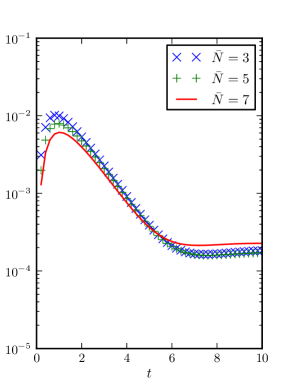
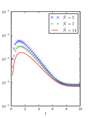
Figure 2. Evolution of the numerical relative $L^{1}$ error of the fast DVM method for $N=32$ (left) and $N=64$ (right) grid points.

We then compare in Figure 2 the time evolution of this error, still in $L^{1}$ norm. We can see that it increases initially (exactly as in the classical and fast spectral methods [17]), and then decreases monotonically in time. A saturation phenomenon due to aliasing errors finally occurs as for the fast spectral method (see [17], Figure 1).

We then give the computational cost of the classical and fast DVM methods in Table 2. Here one can see the drastic improvement when comparing the two methods: taking e.g. $N=64$ points in each direction, the fast method is more than $28$ time faster than the classical one when no truncation is done (i.e. when we take $\bar{N}=\tilde{N}=14$), and even $109$ times faster with a small loss of accuracy when taking $\bar{N}=7$.

We also present the evolution of these computational times with respect to the total number of points in Figure 3. It is clear when we look at the interpolant curve that the theoretical predictions and the effective computational costs agree perfectly. When $\bar{N}$ is fixed, the fast DVM method is of order $N^{2}\log(N)$ whereas when $N$ is fixed, the dependence in $\bar{N}$ is very close to $\bar{N}^{2}$ (actually, the slope of the interpolant curve is about $1.9$).

Number of	Classical	Fast DVM	Fast DVM	Fast DVM	Fast DVM
points $N$	DVM	with $\bar{N}=3$	with $\bar{N}=7$	with $\bar{N}=14$	with $\bar{N}=28$
$16$	2 s. 95	0 s. 5	x	x	x
$32$	2 min. 18 s.	3 s. 19	14 s. 52	x	x
$64$	133 min. 44 s.	16 s. 2	73 s. 4	4 min. 43 s.	x
$128$	x	85 s. 8	6 min. 18 s.	23 min. 2 s.	92 min. 11 s.

Table 2. Comparison of the computational time between the classical DVM method and the fast DVM method with different values of $\bar{N}$ at time $T=1$ ($\Delta t=0.01$).

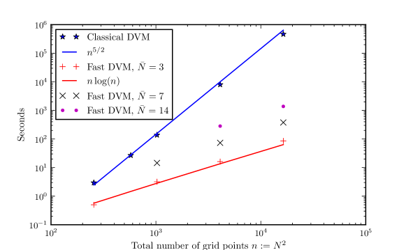
Figure 3. Evolution of the computational time with respect to the total number of points for the classical and fast DVM methods, at time $T=1$

5. Conclusions

We have presented a deterministic way for computing the Boltzmann collision operator with fast algorithms. The method is based on a Carleman-like representation of the operator that allows to express it as a combination of convolutions (this is trivially true for the loss part but it is not trivial for the gain part). A suitable periodized truncation of the operator is then used to derive fast algorithms for computing discrete velocity models (DVM). This can be adapted to any DVM, provided it features a decoupling properties on the quadrature nodes. Our approach will bring the overall cost in dimension $d$ to $O(\bar{N}^{d}N^{d}\log_{2}N)$ where $N$ is the size of the velocity grid and $\bar{N}$ is the size of the grid used to compute directions in the approximation of the discrete operator. Numerical evidences show that the quantity $\bar{N}$ can be taken small compared to $N$. Consistency and accuracy of the proposed schemes are also presented, both theoretically and numerically.

Acknowledgments. The first author wishes to thank Bruno Sévennec for fruitful discussions on the Farey series. The third author wishes to thank Francis Filbet for fruitful discussions and comments about the implementation of the numerical method.

References

- [1] Bobylev, A., and Rjasanow, S. Difference scheme for the Boltzmann equation based on the fast Fourier transform. European J. Mech. B Fluids 16, 2 (1997), 293–306.
- [2] Bobylev, A. V. Exact solutions of the Boltzmann equation. Dokl. Akad. Nauk SSSR 225, 6 (1975), 1296–1299.
- [3] Bobylev, A. V., Palczewski, A., and Schneider, J. On approximation of the Boltzmann equation by discrete velocity models. C. R. Acad. Sci. Paris Sér. I Math. 320, 5 (1995), 639–644.
- [4] Bobylev, A. V., and Rjasanow, S. Fast deterministic method of solving the Boltzmann equation for hard spheres. Eur. J. Mech. B Fluids 18, 5 (1999), 869–887.
- [5] Bobylev, A. V., and Rjasanow, S. Numerical solution of the boltzmann equation using a fully conservative difference scheme based on the fast fourier transform. Transport Theory Statist. Phys. 29, 3-5 (2000), 289–310.
- [6] Bobylev, a. V., and Vinerean, M. C. Construction of Discrete Kinetic Models with Given Invariants. J. Statist. Phys. 132, 1 (Apr. 2008), 153–170.
- [7] Buet, C. A discrete-velocity scheme for the Boltzmann operator of rarefied gas dynamics. Transport Theory Statist. Phys. 25, 1 (Jan. 1996), 33–60.
- [8] Cabannes, H., Gatignol, R., and Luo, L.-S. The Discrete Boltzmann Equation (Theory and Applications). University of California, College of engineering, Los-Angeles, 2003.
- [9] Canuto, C., Hussaini, M. Y., Quarteroni, A., and Zang, T. A. Spectral methods in fluid dynamics. Springer Series in Computational Physics. Springer-Verlag, New York, 1988.
- [10] Carleman, T. Sur la théorie de l’équation intégrodifférentielle de Boltzmann. Acta Math. 60, 1 (1933), 91–146.
- [11] Cercignani, C. Theory and application of the Boltzmann equation. Elsevier, New York, 1975.
- [12] Cercignani, C., Illner, R., and Pulvirenti, M. The mathematical theory of dilute gases, vol. 106 of Applied Mathematical Sciences. Springer-Verlag, New York, 1994.
- [13] Cooley, J. W., and Tukey, J. W. An algorithm for the machine calculation of complex Fourier series. Math. Comp. 19 (1965), 297–301.
- [14] Coquel, F., Rogier, F., and Schneider, J. A deterministic method for solving the homogeneous Boltzmann equation. Rech. Aérospat., 3 (1992), 1–10.
- [15] Filbet, F., Hu, J. W., and Jin, S. A Numerical Scheme for the Quantum Boltzmann Equation Efficient in the Fluid Regime. ESAIM Math. Model. Numer. Anal. 42 (2012), 443–463.
- [16] Filbet, F., and Mouhot, C. Analysis of spectral methods for the homogeneous Boltzmann equation. Trans. Amer. Math. Soc. 363, 4 (2011), 1947–1980.
- [17] Filbet, F., Mouhot, C., and Pareschi, L. Solving the Boltzmann Equation in N log2N. SIAM J. Sci. Comput. 28, 3 (2006), 1029.
- [18] Gamba, I., and Tharkabhushanam, S. H. Spectral-Lagrangian methods for collisional models of non-equilibrium statistical states. J. Comput. Phys. 228 (2009), 2012–2036.
- [19] Hardy, G. H., and Wright, E. M. An introduction to the theory of numbers, sixth ed. Oxford University Press, Oxford, 2008. Revised by D. R. Heath-Brown and J. H. Silverman, With a foreword by Andrew Wiles.
- [20] Hu, J., and Ying, L. A fast spectral algorithm for the quantum Boltzmann collision operator. preprint (2011).
- [21] Ibragimov, I., and Rjasanow, S. Numerical solution of the Boltzmann equation on the uniform grid. Computing 69, 2 (2002), 163–186.
- [22] Kowalczyk, P., Palczewski, A., Russo, G., and Walenta, Z. Numerical solutions of the Boltzmann equation: comparison of different algorithms. Eur. J. Mech. B Fluids 27 (2008), 62–74.
- [23] Krook, M., and Wu, T. T. Exact solutions of the Boltzmann equation. Physics of Fluids 20, 10 (1977), 1589.
- [24] Markowich, P., and Pareschi, L. Fast, conservative and entropic numerical methods for the Boson Boltzmann equation. Numerische Math. 99 (2005), 509–532.
- [25] Martin, Y.-L., Rogier, F., and Schneider, J. Une méthode déterministe pour la résolution de l’équation de Boltzmann inhomogène. C. R. Acad. Sci. Paris Sér. I Math. 314, 6 (1992), 483–487.
- [26] Michel, P., and Schneider, J. Approximation simultanée de réels par des nombres rationnels et noyau de collision de l’équation de Boltzmann. Comptes Rendus de l’Académie des Sciences - Series I - Mathematics 330, 9 (May 2000), 857–862.
- [27] Mouhot, C., and Pareschi, L. Fast methods for the Boltzmann collision integral. C. R. Acad. Sci. Paris Sér. I Math. 339, 1 (2004), 71–76.
- [28] Mouhot, C., and Pareschi, L. Fast algorithms for computing the Boltzmann collision operator. Math. Comp. 75, 256 (2006), 1833–1852 (electronic).
- [29] Nogueira, A., and Sevennec, B. Multidimensional Farey partitions. Indag. Math. (N.S.) 17, 3 (2006), 437–456.
- [30] Panferov, V. A., and Heintz, A. G. A New Consistent Discret-Velocity Model for the Boltzmann Equation. Math. Models Methods Appl. Sci. 25, 7 (2002), 571–593.
- [31] Pareschi, L., and Perthame, B. A Fourier spectral method for homogeneous Boltzmann equations. In Proceedings of the Second International Workshop on Nonlinear Kinetic Theories and Mathematical Aspects of Hyperbolic Systems (Sanremo, 1994), Transport Theory Statist. Phys. (1996), vol. 25, pp. 369–382.
- [32] Pareschi, L., and Russo, G. Numerical solution of the Boltzmann equation. I. Spectrally accurate approximation of the collision operator. SIAM J. Numer. Anal. 37, 4 (2000), 1217–1245.
- [33] Pareschi, L., and Russo, G. On the stability of spectral methods for the homogeneous Boltzmann equation. In Proceedings of the Fifth International Workshop on Mathematical Aspects of Fluid and Plasma Dynamics (Maui, HI, 1998), Transport Theory Statist. Phys. (2000), vol. 29, pp. 431–447.
- [34] Płatkowski, T., and Illner, R. Discrete velocity models of the Boltzmann equation: a survey on the mathematical aspects of the theory. SIAM Rev. 30, 2 (1988), 213–255.
- [35] Platkowski, T., and Walús, W. An acceleration procedure for discrete velocity approximation of the Boltzmann collision operator. Comp. Math. Appl. 39 (2000), 151–163.
- [36] Rogier, F., and Schneider, J. A direct method for solving the Boltzmann equation. Transport Theory Statist. Phys. 23, 1-3 (1994), 313–338.
- [37] Valougeorgis, D., and Naris, S. Acceleration schemes of the discrete velocity method: Gaseous flows in rectangular microchannels. SIAM J. Sci. Comput. 25 (2003), 534–552.
- [38] Villani, C. A review of mathematical topics in collisional kinetic theory. Elsevier Science, 2002.
C. Mouhot
DPMMS, Centre for Mathematical Sciences
University of Cambridge
Wilberforce Road
Cambridge CB3 0WA
UNITED KINGDOM
e-mail: C.Mouhot@dpmms.cam.ac.uk
L. Pareschi
DMI, Università di Ferrara
Via Machiavelli 35
I-44121 Ferrara
ITALY
e-mail: lorenzo.pareschi@unife.it
T. Rey
CSCAMM, University of Maryland
CSIC Building, Paint Branch Drive
College Park, MD 20740
USA
e-mail: trey@cscamm.umd.edu