Copyright

by

Author Name Required !!!

2024

The Dissertation Committee for Author Name Required !!!

certifies that this is the approved version of the following dissertation:

Title Required !!!

Committee:

Sanjay Shakkottai, Supervisor

Gustavo de Veciana

Sriram Vishwanath

Christine Julien

John Hasenbein

Title Required !!!

Publication No.  

Author Name Required !!!, Ph.D.

The University of Texas at Austin, 2024

Supervisor: Sanjay Shakkottai

This dissertation is a study on the design and analysis of novel, optimal routing and rate control algorithms in wireless, mobile communication networks. Congestion control and routing algorithms upto now have been designed and optimized for wired or wireless mesh networks. In those networks, optimal algorithms (optimal in the sense that either the throughput is maximized or delay is minimized, or the network operation cost is minimized) can be engineered based on the classic time scale decomposition assumption that the dynamics of the network are either fast enough so that these algorithms essentially see the average or slow enough that any changes can be tracked to allow the algorithms to adapt over time. However, as technological advancements enable integration of ever more mobile nodes into communication networks, any rate control or routing algorithms based, for example, on averaging out the capacity of the wireless mobile link or tracking the instantaneous capacity will perform poorly. The common element in our solution to engineering efficient routing and rate control algorithms for mobile wireless networks is to make the wireless mobile links seem as if they are wired or wireless links to all but few nodes that directly see the mobile links (either the mobiles or nodes that can transmit to or receive from the mobiles) through an appropriate use of queuing structures at these selected nodes. This approach allows us to design end-to-end rate control or routing algorithms for wireless mobile networks so that neither averaging nor instantaneous tracking is necessary, as we have done in the following three networks.

A network where we can easily demonstrate the poor performance of a rate control algorithm based on either averaging or tracking is a simple wireless downlink network where a mobile node moves but stays within the coverage cell of a single base station. In such a scenario, the time scale of the variations of the quality of the wireless channel between the mobile user and the base station can be such that the TCP-like congestion control algorithm at the source can not track the variation and is therefore unable to adjust the instantaneous coding rate at which the data stream can be encoded, i.e., the channel variation time scale is matched to the TCP round trip time scale. On the other hand, setting the coding rate for the average case will still result in low throughput due to the high sensitivity of the TCP rate control algorithm to packet loss and the fact that below average channel conditions occur frequently. In this dissertation, we will propose modifications to the TCP congestion control algorithm for this simple wireless mobile downlink network that will improve the throughput without the need for any tracking of the wireless channel.

Intermittently connected network (ICN) is another network where the classic assumption of time scale decomposition is no longer relevant. An intermittently connected network is composed of multiple clusters of nodes that are geographically separated. Each cluster is connected wirelessly internally, but inter-cluster communication between two nodes in different clusters must rely on mobile carrier nodes to transport data between clusters. For instance, a mobile would make contact with a cluster and pick up data from that cluster, then move to a different cluster and drop off data into the second cluster. On contact, a large amount of data can be transferred between a cluster and a mobile, but the time duration between successive mobile-cluster contacts can be relatively long. In this network, an inter-cluster rate controller based on instantaneously tracking the mobile-cluster contacts can lead to under utilization of the network resources; if it is based on using long term average achievable rate of the mobile-cluster contacts, this can lead to large buffer requirements within the clusters. We will design and analyze throughput optimal routing and rate control algorithm for ICNs with minimum delay based on a back-pressure algorithm that is neither based on averaging out or tracking the contacts.

The last type of network we study is networks with stationary nodes that are far apart from each other that rely on mobile nodes to communicate with each other. Each mobile transport node can be on one of several fixed routes, and these mobiles drop off or pick up data to and from the stationaries that are on that route. Each route has an associated cost that much be paid by the mobiles to be on (a longer route would have larger cost since it would require the mobile to expend more fuel) and stationaries pay different costs to have a packet picked up by the mobiles on different routes. The challenge in this type of network is to design a distributed route selection algorithm for the mobiles and for the stationaries to stabilize the network and minimize the total network operation cost. The sum cost minimization algorithm based on average source rates and mobility movement pattern would require global knowledge of the rates and movement pattern available at all stationaries and mobiles, rendering such algorithm centralized and weak in the presence of network disruptions. Algorithms based on instantaneous contact, on the contrary, would make them impractical as the mobile-stationary contacts are extremely short and infrequent.

Table of Contents

toc

List of Tables

lot List of Figures

lof

Chapter 1 Introduction

Mobile communication networks have one essential problem that differentiates them from more traditional networks like the Internet or WiFi mesh networks. Communication algorithms for those networks are engineered with the assumption that the network dynamics are either slow enough to be tracked or so fast that the algorithms would essentially see the time average. For example, the round-trip time between any two computers in the Internet is now less than 50msecs. This enables an end-to-end congestion controller like the Transport Control Protocol (TCP) to detect network congestion quickly and adjust the transmission rate in response. In this case, the TCP algorithm tracks the congestion inside the network and adjust the transmission rate accordingly. On the other hand, in the based networks, the wireless channel between a base station and a mobile user fluctuates so rapidly over one data frame transmission time so that it can not be tracked; however, the average bit error rate (BER) in each frame is relatively static over multiple frames, and this allows channel coding algorithm with fixed coding rate to be used.

The classic time-scale separation assumption of trackability or averaging no longer holds in mobile networks. Consider a communication network used by soldiers deployed in remote terrains. These soldiers have organized themselves into multiple, geographically separated clusters, and are equipped with wireless communication devices so that they may communicate with others in the same cluster. However, because of the geographical separation and limited range of the wireless transceivers, they must rely on mobile data transporters to carry data between clusters. When a mobile data transport comes into contact with a cluster, it can pick up a large amount of data per contact with that cluster; it can then move to the destination cluster, and drop off that data into that cluster. If a rate control algorithm at the inter-cluster traffic source (inter-cluster traffic has the source and the destination in different clusters) adjusts the source rate by tracking the mobile-cluster contacts and in essence trying to track the instantaneous available inter-cluster communication data rate, then even though there is a temporary large increase in the available inter-cluster rate when the contact is made, there might not be enough rate available within the cluster through which the inter-cluster flow must travel; in effect, only small portion of the large instantaneous inter-cluster rate can be used.

Alternatively, if the rate control algorithm tries to adjust the rates based on the “average” inter-cluster rates, then either there will be a large queue build up at every node (as we will demonstrate in the later chapter) or the algorithm runs into the problem of finding out what the “average” rate is, which makes it weak in the presence of changes and failures in the network.

In this dissertation, we design and analyze novel routing and rate control algorithms in mobile communication networks where tracking or averaging the network dynamics is impossible or leads to inefficient performance. Towards that end, we examine three types of networks; we briefly introduce each type and highlight our contributions below.

1.1 Problem Statements and Contributions

1.1.1 TCP for Wireless Downlink Networks

It is well-known that TCP connections perform poorly over wireless links due to channel fading. To combat this, techniques have been proposed where channel quality feedback is sent to the source, and the source utilizes coding techniques to adapt to the channel state. However, the round-trip timescales quite often are mismatched to the channel-change timescale, thus rendering these techniques to be ineffective in this regime. (By the time the feedback reaches the source, the channel state has changed.)

In this dissertation, we propose a source coding technique that when combined with a queuing strategy at the wireless router, eliminates the need for channel quality feedback to the source. We show that in a multi-path environment (e.g., the mobile is multi-homed to different wireless networks), the proposed scheme enables statistical multiplexing of resources, and thus increases TCP throughput dramatically.

1.1.2 Time-Scale Decoupled Routing and Rate Control in Intermittently Connected Networks

The second type of network we study in this dissertation is an intermittently connected network (ICN) composed of multiple clusters of wireless nodes. Within each cluster, nodes can communicate directly using the wireless links; however, these clusters are far away from each other such that direct communication between the clusters is impossible except through mobile contact nodes. These mobile contact nodes are data carriers that shuffle between clusters and transport data from the source to the destination clusters. Our dissertation here focuses on a queue-based cross-layer technique known as back-pressure algorithm. The algorithm is known to be throughput optimal, as well as resilient to disruptions in the network, making it an ideal candidate communication protocol for our intermittently connected network.

We design a back-pressure routing/rate control algorithm for ICNs. Though it is throughput optimal, the original back-pressure algorithm has several drawbacks when used in ICNs, including long end-to-end delays, large number of potential queues needed, and loss in throughput due to intermittency. We present a modified back-pressure algorithm that addresses these issues.

1.1.3 Efficient Data Transport with Mobile Carriers

For the third type of network, we consider a network of stationary nodes that rely on mobile nodes to transport data between them. We assume the mobile nodes can control their mobility pattern to respond to data traffic loads, as well as satisfy some other secondary objectives, such as surveillance requirements. We study this problem in the framework of cost minimization, and we derive a dual iterative algorithm that results in optimal mobility pattern for minimizing network wide cost.

1.2 Organization

Each subsequent chapter focuses one of the three network types above. In Chapter 2, we study the problem of TCP congestion controller in cellular networks. We briefly discuss the TCP background and present our modifications that will improve the TCP throughput using multi-homing. We then present our simulation results.

Chapter 3 is on rate control and routing in intermittently connectedly network using a back-pressure algorithm. We describe the back-pressure algorithm and highlight the benefits and shortcomings of the algorithm in ICN. We then present our solutions and present our experimental results obtained from our test bed.

In Chapter 4, we present our mobility control algorithm that minimizes the network wide cost. We present our network model and state our cost minimization optimization problem and iterative solution algorithm, followed by our experimental results.

We end this dissertation with a conclusion and a discussion on possible future research topics.

Chapter 2 TCP for Wireless Downlink Networks

2.1 Introduction

The Transport Control Protocol (TCP) is the most widely used congestion control protocol in the Internet. When a router in the Internet is used beyond its capacity, its buffer will overflow and start to drop packets. A source using TCP will interpret dropped packets as a signal of congestion, and it will promptly reduce its transmission rate to relieve the congestion.

TCP was designed and optimized with the assumption that the networks that it was supposed to operate over have highly reliable node-to-node links such that dropped packets due to poor link quality are highly unlikely. Hence, a dropped packet meant only one thing – congestion.

However, in wireless networks, TCP has no way of distinguishing congestion drops and drops due to poor quality wireless channel. A typical wireless link is designed with average BER (Bit Error Rate) on the order of $10^{-5}$, which results in an average packet error/drop probability (PER) of 5-10% assuming 1KB packet. In addition, the average BER (and PER) of a wireless link can fluctuate over time, and the rate of fluctuation poses a significant problem for TCP. If plain TCP is used over the wireless links without any modifications, this considerably reduces TCP’s average congestion window size and prevents it from enlarging the window size to any significant portion of the ideal size, the bandwidth-delay product, resulting in a low utilization rate [32, 40, 6]. Take for example, a plain TCP (Reno) connection made over one-hop wireless link. Suppose the bandwidth-delay product is infinite for this connection. However, the packet drop probability due to bad wireless channel is $d$. In Figure 2.1(a), we plot the average window size of this TCP connection as $d$ varies from 0.001% to 10%. As the figure shows, the average window size (and the throughput) decreases substantially as $d$ increases. A similar performance graph is shown in Figure 5 of [32].

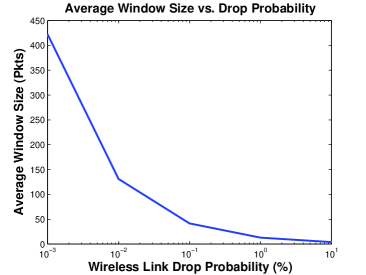
(a) Average window size of plain TCP connection made over one wireless link with packet drop probability $d$ due to fading. As $d$ increases, the average window size and the throughput drops rapidly.

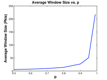
(b) Average window size of TCP using FEC at fixed coding rate as $p$ varies. Even if the coding rate is sufficient for the average channel drop probability, if the drop probability changes every RTT, then the throughput will still be low. The drop probability is equal to 0.05 with probability $p$, and is equal to 0.15 with probability $1-p$.

Figure 2.1: Performance of TCP over one-hop wireless link

In this chapter, we address the problem of low TCP throughput in the simple topology of TCP senders connected via wireline network to intermediate wireless routers and TCP receivers connected by a wireless channel to multiple intermediate routers (see Figure 2.2). An example scenario would be a cellular access network (such as UMTS/WiMax) where the cellular base station is connected to the wired backbone, and only the link between the base station and the mobile user is wireless. Although multi-homing is not currently implemented in current cellular networks, with the introduction of femto-cells, it is conceivable that in a campus scenario with a number of femto-cells, the mobile user may be able to receive downlink data simultaneously on multiple links from multiple femto-cells; this motivates the multi-path model in Figure 2.2.

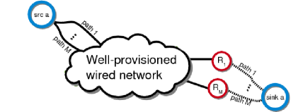
Figure 2.2: A multipath TCP-RLC connection made over a well-provisioned wired network and $M$ wireless routers. We exploit multi-path wireless channel diversity to increase throughput. The dashed lines represent wireless links.

2.1.1 Shortcomings of Existing Solutions

To combat the adverse nature of the wireless network, multiple solutions have been proposed, all involving a separation of time-scales between the rate of channel variation and the TCP congestion window evolution. One can break the TCP connection between a wired server and a mobile into two components: wired and wireless [7]. However, this approach needs a proxy at the wireless base-station, and breaks TCP end-to-end semantics.

By contrast, one could protect TCP (without proxying at the wireless router) from channel-level variations by suitable physical layer schemes. Of these, the commonly deployed solution in UMTS/WiMax systems involves channel coding, adaptive modulation and/or automatic repeat request (ARQ or hybrid ARQ) deployed in a lower layer protocol to deal with packet drops resulting from channel variations that are at a much faster rate than the end-to-end TCP round-trip time (RTT). However, these schemes could lead to variations in the rate provided to the TCP connections, and can lead to suboptimal TCP performance [19]. Papers such as [26] improve TCP performance over downlink wireless networks through dynamically adjusting PHY layer parameters optimized for TCP. However, such strategies require measurements both at the transport layer like TCP sending rate as well as physical layer information like channel quality at the cost of increased complexity at the cellular base station.

The alternate solution (see [10, 75, 71]) is to code the data stream at a specific forward error coding rate at the application layer so that the decoded TCP data stream can withstand drops due to bad wireless channels. In [75], the authors use Reed-Solomon coding at a fixed rate to encode a stream of TCP packets in order to deal with random losses. In [71], the authors use network coding combined with an ACK scheme found in [72] and TCP-Vegas like throughput measurements to adapt TCP over wireless links. However, such an approach requires the variation in channel drop rate to be quasi-static relative to the time-scale of feeding back this channel drop rate information to the source so that the coding rate can be adjusted.

2.1.2 Motivation

Channel Variation and RTT Have Same Time-Scale

In many realistic settings, the packet drop rate of the wireless channel can change at the time scale of round-trip time of the TCP connection. For example, consider a mobile user traveling at 2-5km/h using the current UMTS network (carrier frequency $\approx$ 2GHz in the U.S.). This user’s wireless channel coherence time is roughly around 20-50ms [57], a number well within the range of RTT for the Internet. (Coherence time is roughly a measure of how long a wireless channel stays constant, and therefore a rough measure of how fast the packet drop rate changes.)

In such scenarios, multiple ARQ requests and link-level ACKs and NACKs are unhelpful – they cause retransmission delays and timeouts that may adversely affect the RTT estimation and the retransmission time-out (RTO) mechanism, and therefore throughput. Moreover, forward error correction coding at a fixed rate (at the TCP source) is not helpful since the drop rate at the wireless link is not quasi-static relative to the feedback time scale. If the drop rate changes every RTT, the information about the drop rate will not reach the TCP sender in time to be useful since by the time the information reaches the sender, the drop rate would have changed. Thus, this mobile user’s wireless downlink channel would be useless to track from the perspective of improving his TCP throughput; the channel quality feedback reaches the source too late, and is useless by the time the source gets it.

Take for example a TCP connection made over one wireless link. The packet drop probability due to bad channel conditions changes every RTT time period. Assume that the drop probability $d\in\{0.05,0.15\}$, with the probability that $d=0.05$ is $p$ and the probability that $d=0.15$ is $1-p$. Suppose that the TCP flow uses forward error correction coding at the rate of 10%, i.e. for every 10 data packets, 1 coded packet is generated. Using this FEC coding rate, the TCP data packets can reliably be delivered to the destination if the drop probability $d$ is 0.05. However, because the drop probability can be bad ($d=0.15$) often enough, the TCP throughput will be significantly small. In Figure 2.1(b), we plot the average window size of the TCP connection as we vary $p$. (We assumed that the bandwidth-delay product is infinite.) As the graph shows, even though we have used FEC coding rate that is sufficient for the average drop probability, the throughput is still low because the drop probability changes every RTT.

In summary, coding at fixed rate will not work when the wireless channel variation and TCP RTT have the same time-scale.

Multiple Path Statistical Multiplexing

There has been much research into multipath TCP connections. The obvious advantage of multipath TCP is that it can balance the load on the multiple paths such that paths experiencing temporarily high capacity can carry more packets than paths experiencing low capacity. Further, multiple TCP connections can be useful for load balancing among multiple wireless interfaces – for instance, in a situation where a mobile node is connected to a 3G network base-stations as well as a femto-cell base-station. In this scenario, one would want to get statistical multiplexing gain among the two wireless interfaces, as it is likely that the wireless fading state between the two interfaces will differ (e.g., when the 3G interface has a “bad” channel, the femto-cell interface could have a “good” channel). However to exploit this, a naive implementation would require that packets stored at the 3G base-station be transferred to the other base-station (femto) through a wired back-haul. Clearly, time-scales of RTT over the back-haul and channel variation would render this impractical.

A second issue one faces when running a TCP connection over multiple paths is the problem of out-of-order packet delivery, which can cause congestion window collapse even if the network has plenty of capacity [80]. [54] gets around this problem by delaying and reordering received packets before they are passed up to the TCP layer on the receive side. [83] uses duplicate selective ACKs (DSACK) and dynamically changes the duplicate ACK threshold to address the out-of-order problem.

By using random linear coding, our proposed TCP modifications can be naturally extended to multiple paths, and we will show that coding + TCP enables the network to behave as though packets are “virtually shared” among the different base-stations without the need for a back-haul between the various base-stations. This in-turn leads to multiplexing gains. Further, coding + TCP can easily deal with out-of-order delivery of packets.

2.1.3 Other Related Work

Other coding approaches: Recently, inspired by [1, 37] and others, network coding schemes have been used in the context of wireless networks in order to improve throughput. [21] and [60] use network coding at intermediate nodes and exploit the shared wireless spectrum to improve TCP throughput. In our approach, we use random linear coding (RLC) [45] at the end nodes to improve TCP throughput, and the intermediate router does not perform any coding operations. The concept of using random linear coding for TCP over wired networks has appeared recently [13]; however, our work here is for hybrid network with the goal of improving TCP throughput over time-varying wireless channels.

TCP window statistics under AQM: There is a considerable body of literature [30, 76] on modeling the TCP window process in the presence of active queue management (AQM) systems, especially random early detection (RED) [25]. [76] presents a weak limit of the window size process by proving a weak convergence of triangular arrays. [5] presents a fluid limit of the TCP window process, as the number of concurrent flows sharing a link goes to infinity, and the authors show that the deterministic limiting system provides a good approximation for the average queue size and total throughput. None of the previous works mentioned above treats the situation when the loss rate can not be tracked due mismatch between the channel change time-scale and the RTT time-scale.

This chapter shows throughput gains that can be achieved by multi-path diversity when TCP is combined with an ACK scheme similar to the one in [71] and priority queuing strategy found in [11], plus RLC [45].

2.1.4 Main Contributions

In this work, we employ (i) random linear coding, (ii) priority-based queuing at wireless routers and (iii) multi-path routing to demonstrate that throughput can be increased significantly for TCP over downlink wireless networks even when channel variations are on the same time-scale as RTT. Our theoretical result shows that we can obtain full statistical multiplexing gain from multi-path TCP.

Specifically, our analysis shows that we can achieve TCP throughput of $\Theta\left(\mathbb{E}\left[P\right]C\right)$ in multiple path (multi-homing) case with our modifications, in the absence of channel quality feedback from the destination to the sender. Here, $\mathbb{E}\left[P\right]$ is the mean probability of successful packet transmission of the time-varying wireless channel; $C$ is the capacity of the wireless router.

Further, our modifications to TCP, which we call TCP-RLC, present an orderwise gain over the performance of plain TCP, which is $\Theta(1)$, in the presence of random packet loss for wired-wireless hybrid networks, where the random packet loss rates change at the RTT time scale and cannot be tracked.

2.2 Analytical Model

We consider slotted time. Each time slot is equal to round-trip time between the senders and the receivers. The TCP-RLC source $i$ maintains a congestion window of size $W_{i}(t)$ for the $t$-th RTT interval. The congestion window is in units of packets; packets are assumed to be of fixed size. In each RTT slot, source $i$ wants $W_{i}(t)$ data packets to be transferred to sink $i$. We model the additive increase, multiplicative decrease (AIMD) evolution of the TCP congestion window as follows:

$$W_{i}(t+1) = \mathbf{1}_{\text{success}}\left(W_{i}(t)+1\right)+\mathbf{1}_{\text{drop}}\left\lceil W_{i}(t)/2\right\rceil$$

$$= W_{i}(t)+1-\mathbf{1}_{\text{drop}}\left\lfloor 1+W_{i}(t)/2\right\rfloor$$

where the random variable $\mathbf{1}_{\text{success}}\mbox{$\stackrel{{\scriptstyle\small\Delta}}{{=}}$}1$ when all data packets transmitted in the $t$-th RTT interval for destination $i$ have been successfully received at the destination; $\mathbf{1}_{\text{drop}}\mbox{$\stackrel{{\scriptstyle\small\Delta}}{{=}}$}1-\mathbf{1}_{\text{success}}$ takes the value $1$ when either (i) the receiver cannot recover one or more data packets corrupted by the packet drop process or (ii) a packet is marked by the router due to the presence of an active queue manager (AQM). AQM marks a connection with window size $W$ according to the probability given by $f(W)$, and thus the congestion window is deliberately halved.

In our analytical model, we assume that the routers can measure the window size $W$ of a TCP flow, and based on the window size, each router can mark the flow with probability $f(W)$. If a flow is marked by a router, the TCP source halves the TCP window size $W(t)$ and reduces the transmission rate by factor of two.

We let $f(W)$ be the probability that a flow is marked when the window size is $W$, and we let $f_{\text{chan}}(W)$ denote the probability that the destination is unable to reconstruct the $W$ data packets due the channel packet drop/corruption processes over all paths, which would halve the TCP congestion window.

The combined effects of the AQM with the marking function $f(w)$ and the packet drops from the wireless channels can be encapsulated into $f_{\text{eff}}(w)$ where

$$f_{\text{eff}}(w) = 1-(1-f_{\text{eff}}(w))$$ (2.2)

$$= 1-(1-f(w))(1-f_{\text{chan}}(w))$$

$$= f(w)+f_{\text{chan}}(w)-f(w)f_{\text{chan}}(w).$$

Thus, the TCP congestion window will decrease by half or increase by one with probabilities $f_{\text{eff}}(w)$ and $1-f_{\text{eff}}(w)$, respectively, if the window size is $w$.

In this chapter, we are interested in finding the average throughput under the optimal AQM, i.e. $\mathbb{E}\left[W^{*}(t)\right]$, where $W^{*}(t)$ is the congestion window under the AQM that maximizes $\mathbb{E}\left[W^{*}(t)\right]$. Note that the optimal AQM may be no AQM at all, but throughput under the optimal AQM has to be greater than that under some arbitrary AQM. The presence of AQM greatly simplifies our analysis. We later back our claims with simulation results that used no AQM.

In practical scenarios, the evolution of the congestion window size is limited by the sender/receiver buffer size; we will ignore this to simplify our analysis. We will also neglect TCP timeouts for the same reason.

2.2.1 Random Linear Coding

In each time slot, the source $i$ takes $W_{i}(t)$ data packets and generates $rW_{i}(t)$ ($r>0$) coded packets as follows: let each data packet $x_{ik},k=1,2,\ldots,W_{i}(t)$ be represented as an element of some finite field $\mathbb{F}_{q}$; choose elements $\alpha_{ikj}\in\mbox{$\mathbb{F}_{q}$}$ uniformly at random and generate a coded packet

$$y_{ij}=\sum_{k=1}^{W_{i}(t)}\alpha_{ikj}x_{ik}$$

for $j=1,2,\ldots,rW_{i}(t)$. The receiver can decode, with very high probability, any dropped data packets if sufficient number of linearly independent coded and data packets are received, as the field size from which the coding coefficients are drawn increases. Hence, in the rest of the work, we will make the following assumption as a simplification.

Assumption 1.

Suppose $W$ data packets are used to generate coded packets via RLC. If $G$ coded packets are received by the TCP destination, then upto $G$ missing data packets out of the $W$ data packets can be recovered.

Thus, if the number of missing data packets from $W$ exceeds $G$ in an RTT slot, the congestion window will halve (and $\mathbf{1}_{\text{drop}}=1$). That is, if $G$ coded packets received and as long as no more than $G$ data packets of the original $W$ data packets are lost, then the receiver can recover all of the original data. For detailed exposition on RLC and justification of assumption 1, see [46].

2.2.2 Network Topology

The network topology we consider in this chapter is a TCP-RLC connection made over $M\geq 1$ paths going through router $R_{1}$,…, $R_{M}$, each with capacity $C$ (black connection in Figure 2.2). Only the link between $R_{i}$, $i=1,...,M$ and the destination is wireless; the links between the routers and the source are wired. The well-provisioned wired network is assumed with the paths having the same RTT, and the wireless routers do not store packets from one RTT slot to another in the analytical mode. In practice, the paths will have different, but similar, RTT values.

We assume that the wired section of the network has greater capacity than the wireless section. This is a reasonable assumption, since all of the currently existing downlink networks have wired back-plane network with excess capacity, and the wireless downlink channel is greatly limited due to tight spectrum and power constraints.

2.2.3 Wireless Downlink Channel

We model packet drops in the wireless channel between a wireless router and the TCP-RLC destination as a simple i.i.d. packet drop process whose parameter remains constant for each RTT-interval. This is similar to the block-noise model common in wireless communication literature.

Within each RTT-interval $t$, the probability that a packet transmitted over the air by the wireless router $i\in\{1,...,M\}$ for the destination is successfully received is given by $p_{i}(t)$. The $j$-th packet transmitted over the air by the wireless router $i$ for the destination is corrupted (dropped) according to a Bernoulli error process $H_{j}^{i}(t)$ defined as

$$H_{j}^{i}(t)=\left\{\begin{array}[]{ll}1&\textnormal{w.p. $p_{i}(t)$ if }j^{\textnormal{th}}\textnormal{ packet is received correctly}\\ 0&\textnormal{w.p. $1-p_{i}(t)$ if }j^{\textnormal{th}}\textnormal{ packet dropped}\end{array}\right.$$

with parameter $p_{i}(t)\in\{p_{1}=p_{\min},p_{2},\ldots,p_{\Pi}=p_{\max}\}$ acting upon each packet over the air independently of other packets in the same RTT-interval. We assume that $p_{1}>0$ and $p_{1}<p_{2}<\ldots<p_{\Pi}$. We assume that $p_{i}(t)$ changes over time with $\mathbb{P}(p_{i}(t)=p_{k})=\tilde{p}_{k}$. Thus, the channel packet-delivery-probability parameter itself changes with time (this corresponds to changing fading state over time), and at any time the actual packet delivery probability depends on the instantaneous value of this (random, time-varying) parameter.

Lastly, we assume that $r>2(1-p_{\min})/p_{\min}$ for multiple paths topology.

2.2.4 Priority Transmission

In the multiple path network topology, the source maintains a path-level congestion window $w_{l}(t)$ for each path $l$; this is in addition to $W(t)$. The idea in our multi-path algorithm is to have a rate control on each path. The transmission rate of the high priority packets on path $l$ is controlled by $w_{l}(t)$. $w_{l}(t)$ will be the number of high priority (data) packets in transit towards the destination in time slot $t$; in addition, there will be $rw_{l}(t)$ low priority (coded) packets that will be in transit as well. If $w_{l}(t)$ packets (either high or low priority) are successfully received by the destination, the rate controller on path $l$ at the source will increase $w_{l}$ by one so that in time slot $t+1$, $w_{l}(t+1)=w_{l}(t)+1$. If not, then $w_{l}$ will be halved, so that $w_{l}(t+1)=w_{l}(t)/2$.

The main idea in our algorithm is to separate the problem of wireless link reliability on each path from the TCP rate control algorithm that operates over all paths ($W(t)$). On each path, the only sign of congestion is if the total number of packets (high + low priority) received by the destination on path $l$ is less than the number of high priority packets it should have received on that path; that is, the router on path $l$ did not have enough capacity to either 1) send all high priority packets it received or 2) send enough low priority coded packets to compensate for any high priority packets that were dropped by the wireless link. Unlike in the of the traditional TCP over wired links, gaps in the sequence of the received packet numbers are not a valid way of measuring congestion over wireless links. The mechanism that acts on $w_{l}(t)$ we described in the previous paragraph is a way to “measure” congestion on each path; $w_{l}(t)$ is the number of packets that path $l$ can guarantee to deliver in time slot $t$ to the destination through the wireless router $l$.

Thus, in time slot $t$, path $l$ can have any $w_{l}(t)$ of the $(1+r)W(t)$ data and coded packets delivered to the receiver. The evolution of $w_{l}(t)$ is similar to $W(t)$:

$$w_{l}(t+1) = \mathbf{1}_{\text{success}}\left(w_{l}(t)+1\right)+\mathbf{1}_{\text{fail}}\left\lceil w_{l}(t)/2\right\rceil$$ (2.3)

where $1_{\text{success}}=1$ if $w_{l}(t)$ packets are successfully received in RTT slot $t$; $1_{\text{fail}}=1-1_{\text{success}}$.

Before the packets are sent out on a path, they are marked either high or low priority. The number of high priority packets sent out in any given RTT slot is equal to $w_{l}(t)$. For each high priority packet sent out, the path transmits $r$ low priority packets.

Note that as long as $W(t)$ data packets are successfully received (or recovered), $W(t)$ will increase according to eq. (2.2). Since the available rates on the $M$ paths ($w_{1}(t)$, $w_{2}(t)$, …, $w_{M}(t)$) evolve independently, we need a way to measure the total available instantaneous rate through all paths combined, and the main purpose of having $W(t)$ is to measure this total, combined rate through all paths. The algorithm at the source is designed such that in time slot $t$, the main rate controller will take $W(t)$ data packets, generate $rW(t)$ coded packets, and leave both types of packets in some memory location. Path-wise rate controller on path $l$ will take $w_{l}(t)$ data packets, mark them high priority, and send them out along with $rw_{l}(t)$ coded packets, which it will mark low priority. If in time slot $t$, $W(t)$ data packets are successfully reconstructed at the destination, the main controller will deduce that the total available rate through all paths is equal to or greater than $W(t)$, and hence $W(t+1)=W(t)+1$. Else, it will deduce the total available rate is less, and $W(t+1)=W(t)/2$.

2.2.5 Wireless Router

We assume that the low priority packets are transmitted by the router only when there are no high priority packets that can be transmitted. For example, in the case $M=1$, the remainder of the nominal channel capacity $C$, $C-w_{1}(t)$, is used to transmit low priority packets in $t$-th RTT slot, where the evolution of $w_{1}(t)$ is defined in eq. (2.3).

We also make the assumption that the wireless router maintains a pair of queues for each TCP-RLC connection made through that router. While such a number that scales with the number of flows would be prohibitive for routers in the Internet core, we argue that it is reasonable for wireless downlink routers, as these routers serve relatively small number of mobile users in the same cell. In addition, per flow queue maintenance is already done in cellular architectures for reasons of scheduling, etc. (see [9]).

For each TCP-RLC connection, one queue (FIFO) is used to handle high priority packets; the other queue (LIFO) is used for low priority packets. (LIFO queue is used for low priority packets because the low priority packets are transmitted only when the router has excess capacity. The router will run out of capacity often enough so that if FIFO is used for low priority packets, then after long enough time, it will be backed up with old low priority packets and any newly arriving low priority packets will be dropped due to (low priority) buffer overflow.) In our analysis, we assumed that packets are not stored in the router’s queues from one RTT time slot to another. We relax this in our simulations.

2.3 Multiple Path Analysis

We first analyze the evolution of path-level congestion window. Given that the path-level window size is $w_{l}(t)$ for path $l$ in time slot $t$, $w_{l}(t+1)=\lceil w_{l}(t)/2\rceil$ if out of the $C$ packets transmitted by the router, fewer than $w_{l}(t)$ packets with the same block number are received; let $\chi_{\text{fail}}$ be this event.

Using Chernoff’s bound, we can show for any $\epsilon>0$,

$$\mathbb{P}\left[\chi_{\text{fail}}|p_{l}(t)=p_{1},~{}w_{l}(t)<(1-\epsilon)p_{1}C\right]\leq\exp(-\epsilon^{2}p_{1}C/2)$$

Similarly, we can show that

$$\mathbb{P}\left[\chi_{\text{fail}}|p_{l}(t)=p_{1},~{}w_{l}(t)>(1+\epsilon)p_{1}C\right]\geq 1-\exp(-\epsilon^{2}p_{1}C/2).$$

In addition, it is straight forward to show that for any $i=2,...,\Pi$,

$$\mathbb{P}\left[\chi_{\text{fail}}|p_{l}(t)=p_{i},~{}w_{l}(t)<(1-\epsilon)p_{1}C\right]\leq\mathbb{P}\left[\chi_{\text{fail}}|p_{l}(t)=p_{1},~{}w_{l}(t)<(1-\epsilon)p_{1}C\right]$$

since $p_{1}<p_{i}$. Thus,

$$\mathbb{P}\left[\chi_{\text{fail}}|w_{l}(t)<(1-\epsilon)p_{1}C\right] \leq \sum_{i=1}^{\Pi}\tilde{p}_{i}\exp(-\epsilon^{2}p_{1}C/2)$$ (2.4)

$$= \exp(-\epsilon^{2}p_{1}C/2)$$

and

$$\mathbb{P}\left[\chi_{\text{fail}}|w_{l}(t)>(1+\epsilon)p_{1}C\right] \geq \mathbb{P}\left[\chi_{\text{fail}}|p_{l}(t)=p_{1},~{}w_{l}(t)>(1+\epsilon)p_{1}C\right]$$ (2.5)

$$= \tilde{p}_{1}(1-\exp(-\epsilon^{2}p_{1}C/2)).$$

From eqs. (2.4), (2.5) and (2.3), we see that $0.5(1-\epsilon)p_{1}C\leq w_{l}(t)\leq(1-\epsilon)p_{1}C$ w.p. at least $1-\exp(-\epsilon^{2}p_{1}C)$. Since $(1+r)w_{l}(t)$ high and low priority packets are sent on path $l$ and $r>2(1-p_{1})/p_{1}$, the wireless router on path $l$ sends $C$ in each time slot w.p. at least $1-\exp(-\epsilon^{2}p_{1}C)$.

In a network with $M$ paths, the probability that $0.5(1-\epsilon)p_{1}C\leq w_{l}(t)\leq(1-\epsilon)p_{1}C$, $\forall l=1,...,M$ is at least $(1-\exp(-\epsilon^{2}p_{1}C))^{M}\geq 1-M\exp(-\epsilon^{2}p_{1}C)$ where $C>>M$. Thus, we make the following reasonable assumption:

Assumption 2.

On each path $l=1,...,M$, the wireless router transmits $C$ (high + low priority) packets to the TCP-RLC destination in each time slot.

From assumption 2, we have that $W(t)$ is an irreducible, aperiodic Markov chain; $W(t+1)$ depends only on $W(t)$ and $p_{l}(t)$, $l=1,...,M$. Let $\pi_{W}$ denote its stationary distribution.

Let $\chi_{\textnormal{failure}}^{\prime}=\left\{\sum_{k=1}^{M}\sum_{j=1}^{C}H_{j}^{k}(t)<W(t)\right\}$. Fix $\rho>1$ and let $\Upsilon$ denote the event $\left\{\frac{1}{M}\sum_{i=1}^{M}p_{i}(t)\geq\frac{\rho W(t)}{MC}\right\}$. Then

$$f_{\textnormal{chan}}(W(t)) = \mathbb{P}\left[\Upsilon\right]\mathbb{P}\left[\chi_{\textnormal{failure}}^{\prime}|\Upsilon\right]+\mathbb{P}\left[\neg\Upsilon\right]\mathbb{P}\left[\chi_{\textnormal{failure}}^{\prime}|\neg\Upsilon\right].$$

Lemma 1.

$f_{\textnormal{chan}}(w)$ can be bounded as below

$$f_{\textnormal{chan}}(w)\leq\left\{\begin{array}[]{ll}\exp\left(-MCL_{1}\right)\text{ if }0\leq\frac{\rho^{2}w}{MC}\leq p_{1}&\\ \exp\left(-MCL_{2}\right)+\exp\left(-Ml^{\prime}\left(1-\frac{\rho w}{MC}\right)\right)\text{ if }p_{1}<\frac{\rho^{2}w}{MC}<\mathbb{E}\left[P\right]\end{array}\right.$$

where $L_{1}$ and $L_{2}$ are non-zero constants, and

$$l^{\prime}(a)=\max_{-\infty<\Theta<\infty}\left\{\Theta a-\log M^{\prime}(\Theta)\right\}$$ (2.7)

and $M^{\prime}(\Theta)=\mathbb{E}\left[e^{\Theta(1-P)}\right]$.

Proof: Let $\widehat{p}(t)=\frac{1}{M}\sum_{i=1}^{M}p_{i}(t)$. If $p_{1}\leq\frac{\rho^{2}W(t)}{MC}<\mathbb{E}\left[P\right]$, by Chernoff’s bound

$$\mathbb{P}\left[\neg\Upsilon\right] = \mathbb{P}\left[\frac{1}{M}\sum_{i=1}^{M}\left(1-p(i,t)\right)>1-\frac{\rho W(t)}{MC}\right]$$

$$\leq \exp\left(-Ml^{\prime}\left(1-\frac{\rho W(t)}{MC}\right)\right).$$

Then,

$$\mathbb{P}\left[\chi_{\textnormal{failure}}^{\prime}|\Upsilon\right] \leq \mathbb{P}\left[\chi_{\textnormal{failure}}^{\prime}|\widehat{p}(t)=\frac{\rho W(t)}{MC}\right]$$ (2.8)

$$\leq e^{\left(-MCD\left(1-\frac{W(t)}{MC}||1-\frac{\rho W(t)}{MC}\right)\right)}$$ (2.9)

where $D(x||y)$ is the Kullback-Leibler distance between $x$ and $y$; eq. (2.8) follows because lowering $\widehat{p}(t)$ will increase the probability that the transmission will not be successful, and eq. (2.9) by Chernoff’s bound.

Let $L_{1}=\inf_{W:p_{1}\leq\frac{\rho^{2}W}{MC}\leq\mathbb{E}\left[P\right]}D\left(1-\frac{W}{MC}||1-\frac{\rho W}{MC}\right)$. Thus, if $p_{1}\leq\frac{\rho^{2}W(t)}{MC}<\mathbb{E}\left[P\right]$, we have

$$f_{\textnormal{chan}}(W)\leq\exp\left(-Ml^{\prime}\left(1-\frac{\rho W}{MC}\right)\right)+\exp\left(-MCL_{1}\right)$$

since $\mathbb{P}\left[\Upsilon\right],\mathbb{P}\left[\chi_{\textnormal{failure}}^{\prime}|\neg\Upsilon\right]\leq 1$.

If $\frac{\rho^{2}W(t)}{MC}<p_{1}$, we have $\mathbb{P}\left[\Upsilon\right]=1$ because $\hat{p}(t)\geq p_{1}$. In addition,

$$\mathbb{P}\left[\chi_{\text{failure}}^{\prime}|\Upsilon\right] \leq \mathbb{P}\left[\chi_{\text{failure}}^{\prime}|\widehat{p}(t)=p_{1}\right]$$ (2.10)

$$\leq e^{\left(-MCD\left(1-\frac{W(t)}{MC}||1-p_{1}\right)\right)}.$$ (2.11)

Inequality (2.10) follows from the fact that decreasing the probability that $H_{j}^{i}=1$ will increase the probability that not enough packets will be received by the receiver to decode $w$ packets. Inequality (2.11) follows from Chernoff bound. Let $L_{2}=\inf_{w:\frac{\rho^{2}w}{MC}\in[0,p_{1})}D\left(1-\frac{w}{MC}||1-p_{1}\right)$. Then

$$\mathbb{P}\left[\chi_{\text{failure}}^{\prime}|\Upsilon\right]\leq\exp\left(-MCL_{2}\right),$$

and

$$f_{\textnormal{chan}}(W)\leq\exp\left(-MCL_{2}\right)$$

in the region $\frac{\rho^{2}W(t)}{MC}<p_{1}$ since $\mathbb{P}\left[\neg\Upsilon\right]=0$  

Theorem 1.

Fix $\rho>1$ and $M$. Then,

$$\mathbb{E}\left[W^{*}(t)\right] \geq \max\left\{0.75p_{1}MC/\rho^{2}-1,\min\left\{\frac{\mathbb{E}\left[P\right]MC}{\rho^{2}}\left[1-3\delta_{1}-2\left(e^{-1}+\delta_{2}\right)\right],\right.\right.$$

$$\left.\left.\beta\left[1-3\lfloor\beta\rfloor^{-1}-2\left(e^{-1}+\delta_{2}\right)\right]\right\}\right\}$$

where $\delta_{1},\delta_{2}\rightarrow 0$ as $C\rightarrow\infty$ and where $\beta\in[p_{1}MC/\rho^{2},\mathbb{E}\left[P\right]MC/\rho^{2}]$ is the solution to the equality

$$1/\beta=\exp\left(-Ml^{\prime}(1-\rho\beta/MC)\right)$$ (2.12)

(for $M$, $C$ large enough, we can show a solution exists) and where $l^{\prime}(\cdot)$ is defined in equation (2.7).

Proof: If $\exists\beta\in[p_{1}MC/\rho^{2},\mathbb{E}\left[P\right]MC/\rho^{2}]$ such that $\beta$ is the solution to eq. (2.12), then this case corresponds to the situation when there are enough paths to start gaining path diversity, but not enough paths to gain complete path diversity. (We assume $C$ is large enough so that $l^{\prime}(1-\mathbb{E}\left[P\right]/\rho)<CL$.)

Let

$$f(w)=\left\{\begin{array}[]{ll}\frac{2(\beta)^{-1}-f_{\textnormal{chan}}(w)}{1-f_{\textnormal{chan}}(w)}&\mbox{if $w<\lfloor\beta\rfloor$}\\ 1&\mbox{if $w\geq\lfloor\beta\rfloor$}\end{array}\right.$$ (2.15)

so that $f_{\text{eff}}(w)=2\beta^{-1}$ if $w<\lfloor\beta\rfloor$ and 1 if $w\geq\lfloor\beta\rfloor$. Under this AQM marking scheme,

$$\mathbb{E}\left[W(t+1)\right] = \mathbb{E}\left[W(t)+1\right]-\mathbb{E}\left[1_{\text{drop}}\lfloor 1+W(t)/2\rfloor\right]$$

$$1 = \mathbb{E}\left[f_{\text{eff}}(W)\lfloor 1+W(t)/2\rfloor\right]$$

$$1 \leq \mathbb{E}\left[f_{\text{eff}}(W)(1+W(t)/2)\right]$$

$$1 \leq \mathbb{E}\left[f_{\text{eff}}(W)\right]+\mathbb{E}\left[f_{\text{eff}}(W)W/2\right].$$

Thus,

$$\mathbb{E}\left[f_{\text{eff}}(W)\right]=2\beta^{-1}+(1-2\beta^{-1})\pi_{W}\left(\lfloor\beta\rfloor\right)$$

and

$$\mathbb{E}\left[f_{\text{eff}}(W)\frac{W}{2}\right]=\beta^{-1}\mathbb{E}\left[W\right]+(1-2\beta^{-1})\frac{\lfloor\beta\rfloor}{2}\pi_{W}\left(\lfloor\beta\rfloor\right).$$ (2.16)

Let $S_{k}(t)=1$ if $W(t)=k$ and 0 if $W(t)\neq k$. For $k>\lfloor\lfloor\beta\rfloor/2\rfloor$, we have

$$\mathbb{P}\left[S_{k}(t)\right] = \mathbb{P}\left[S_{k-1}(t-1)\right]\mathbb{P}\left[W(t)=k|W(t-1)=k-1\right]$$

$$= (1-2\beta^{-1})\mathbb{P}\left[S_{k-1}(t-1)\right].$$

Thus,

$$\mathbb{P}\left[S_{\lfloor\beta\rfloor}\left(t+\lceil\lfloor\beta\rfloor/2\rceil\right)\right] = \mathbb{P}\left[S_{\lfloor\lfloor\beta\rfloor/2\rfloor-1}(t)\right]\prod_{k=\lfloor\lfloor\beta\rfloor/2\rfloor}^{\lfloor\beta\rfloor}\mathbb{P}\left[W=k|W=k-1\right]$$

$$= (1-2(\beta)^{-1})^{\lceil\lfloor\beta\rfloor/2\rceil}\mathbb{P}\left[S_{\lfloor\lfloor\beta\rfloor/2\rfloor-1}(t)\right].$$

Let $T_{\lfloor\lfloor\beta\rfloor/2\rfloor-1}$ be the time takes $W(t)$ to return to $\lfloor\lfloor\beta\rfloor/2\rfloor-1$. It is known that

$$\mathbb{P}\left[S_{\lfloor\lfloor\beta\rfloor/2\rfloor-1}(t)\right]=\mathbb{E}_{\lfloor\lfloor\beta\rfloor/2\rfloor-1}\left[T_{\lfloor\lfloor\beta\rfloor/2\rfloor-1}\right]^{-1}.$$

If starting from state $\lfloor\lfloor\beta\rfloor/2\rfloor-1$, the window size increases by $k\geq 0$ before halving, the total number of steps before $W(t)$ returns to $\lfloor\lfloor\beta\rfloor/2\rfloor-1$ is at least $k+\lfloor\lfloor\beta\rfloor/2\rfloor-1-\lceil(\lfloor\lfloor\beta\rfloor/2\rfloor-1+k)/2\rceil$. Minimizing over $k$, the least number of steps before $W(t)$ enters state $\lfloor\lfloor\beta\rfloor/2\rfloor-1$ again is at least $\lfloor(\lfloor\lfloor\beta\rfloor/2\rfloor-1)/2\rfloor$. Thus, $\mathbb{E}_{\lfloor\lfloor\beta\rfloor/2\rfloor-1}\left[T_{\lfloor\lfloor\beta\rfloor/2\rfloor-1}\right]>\lfloor(\lfloor\lfloor\beta\rfloor/2\rfloor-1)/2\rfloor$ and

$$\mathbb{P}\left[S_{\lfloor\lfloor\beta\rfloor/2\rfloor-1}(t)\right]\leq\left(\lfloor(\lfloor\lfloor\beta\rfloor/2\rfloor-1)/2\rfloor\right)^{-1}.$$

So we have

$$\pi_{W}\left(\lfloor\beta\rfloor\right)\leq\frac{(1-2\beta^{-1})^{\lceil\lfloor\beta\rfloor/2\rceil}}{\left(\lfloor(\lfloor\lfloor\beta\rfloor/2\rfloor-1)/2\rfloor\right)}$$ (2.17)

Combining above with equation (2.3), we get

$$\mathbb{E}\left[f_{\text{eff}}(W)\right] \leq \beta^{-1}+\frac{(1-2\beta^{-1})^{\lceil\lfloor\beta\rfloor/2\rceil+1}}{\left(\lfloor(\lfloor\lfloor\beta\rfloor/2\rfloor-1)/2\rfloor\right)}$$

$$\leq \beta^{-1}+\frac{1}{\left(\lfloor(\lfloor\lfloor\beta\rfloor/2\rfloor-1)/2\rfloor\right)}$$

$$\leq 3\left(\lfloor\beta\rfloor\right)^{-1}.$$

Combining equation (2.16) with equation (2.17), we get

$$\mathbb{E}\left[f_{\text{eff}}(W)\frac{W}{2}\right] = \beta^{-1}\mathbb{E}\left[W\right]+(1-2\beta^{-1})\frac{\lfloor\beta\rfloor}{2}\pi_{W}\left(\lfloor\beta\rfloor\right)$$

$$\leq \beta^{-1}\mathbb{E}\left[W\right]+\frac{\lfloor\beta\rfloor}{2}\frac{(1-2\beta^{-1})^{\lceil\lfloor\beta\rfloor/2\rceil+1}}{\left(\lfloor(\lfloor\lfloor\beta\rfloor/2\rfloor-1)/2\rfloor\right)}$$

Since $(1-2\beta^{-1})^{\lceil\lfloor\beta\rfloor/2\rceil+1}$ converges to $e^{-1}$, we have

$$\mathbb{E}\left[f_{\text{eff}}(W)\frac{W}{2}\right]\leq\beta^{-1}\mathbb{E}\left[W\right]+2(e^{-1}+\delta)$$

where $\delta$ is some small, positive constant. Combining the bounds on $\mathbb{E}\left[f_{\text{eff}}(W)\frac{W}{2}\right]$ and $\mathbb{E}\left[f_{\text{eff}}(W)\right]$ and substituting into inequality (2.3), we get

$$1\leq 3(\lfloor\beta\rfloor)^{-1}+\beta^{-1}\mathbb{E}\left[W\right]+2(e^{-1}+\delta).$$

Solving for $\mathbb{E}[W]$ and using $\mathbb{E}\left[W^{*}(t)\right]\geq\mathbb{E}\left[W(t)\right]$, we get

$$\beta\left[1-3\lfloor\beta\rfloor^{-1}-2\left(e^{-1}+\delta_{2}\right)\right]\leq\mathbb{E}[W^{*}].$$

If $\nexists\beta\in[p_{1}MC/\rho^{2},\mathbb{E}\left[P\right]MC/\rho^{2}]$ such that $1/\beta=\exp\left(-Ml^{\prime}(1-\rho\beta/MC)\right)$, then either $1/\beta<\exp\left(-Ml^{\prime}(1-\rho\beta/MC)\right)$ for $\beta=p_{1}MC/\rho^{2}$, or $1/\beta>\exp\left(-Ml^{\prime}(1-\rho\beta/MC)\right)$ for $\beta=\mathbb{E}\left[P\right]MC/\rho^{2}$.

If $1/\beta<\exp\left(-Ml^{\prime}(1-\rho\beta/MC)\right)$ for $\beta=p_{1}MC/\rho^{2}$, then there are not enough paths to gain path diversity. We can use no AQM (i.e., $f(W)=0,\forall W$), and we will be guaranteed throughput at least $0.75p_{1}C/\rho^{2}-1$ as $C\rightarrow\infty$.

If $1/\beta>\exp\left(-Ml^{\prime}(1-\rho\beta/MC)\right)$ for $\beta=\mathbb{E}\left[P\right]MC/\rho^{2}$, then there are sufficient number of paths to gain all path diversity.

Let $\beta=\left(\frac{\mathbb{E}\left[P\right]}{\rho^{2}}MC\right)$ and let

$$f(w)=\left\{\begin{array}[]{ll}\frac{2\beta^{-1}-f_{\textnormal{chan}}(w)}{1-f_{\textnormal{chan}}(w)}&\mbox{if $w<\beta$}\\ 1&\mbox{if $w\geq\beta$,}\end{array}\right.$$

so that $f_{\text{eff}}(w)=\beta^{-1}$ if $w<\beta$ and 1 else. We can follow the same analysis as in the case when the solution to eq. (2.12) exists (just let $\beta$ be equal to $\mathbb{E}\left[P\right]MC/\rho^{2}$ and the result will follow through) and arrive at the conclusion that

$$\mathbb{E}\left[W^{*}(t)\right]\geq\frac{\mathbb{E}\left[P\right]MC}{\rho^{2}}\left[1-3\lfloor\beta\rfloor^{-1}-2\left(e^{-1}+\delta_{2}\right)\right].$$

 

Due to the fact that $w_{l}(t)\leq p_{1}C$ and $r>2(1-p_{1})/p_{1}$, the capacity of the wired section only need to be twice that of the wireless section; i.e. the wired capacity needs to be slightly greater than $2C$.

2.4 Simulation Results

Before we present our simulation results, we note that implementation of TCP-RLC uses novel techniques not found in original version of TCP. We provide brief description of some of the novel techniques in the appendix; we refer any readers interested in the implementation details to the appendix.

We simulate single flow with multiple paths, where we exploit path diversity. In our simulations, the random coefficients used to encode each packet are drawn from a field of size 8191; thus, for coding block size of smaller than $\sim 500$, the probability of two coded packets in the same coding block not being “independent” is negligible. We fixed the size of all packets to 256 bytes. Each flow had two buffers allocated at the router whose capacities were equal to the transmission rate times the RTT. We have used bimodal channel profile, $\left\{(p_{\min},\widetilde{p}_{\min}),(p_{\max},\widetilde{p}_{\max})\right\}$. $p_{\max}$ is set to 1 in all our simulations. We varied $p_{1}$ from 0.1 to 0.5 in increments of 0.1 and set $\widetilde{p}_{1}=0.1$ and $\widetilde{p}_{2}=0.9$. Thus, $\mathbb{E}\left[P\right]$ varied from 0.91 to 0.95. This corresponds to the scenario where the downlink channel can be controlled to provide good capacity most of the time (90% of the time), but bad channel conditions can occur frequently enough to destroy TCP throughput (10% of the time). Note that using fixed coding rate adjusted for the average channel quality would not work for this scenario; coding is not needed most of the time and becomes useless when needed because the coding rate is insufficient against poor quality channel conditions that can occur frequently enough. We varied the number of paths from 1 to 8. We set the total capacity to 1Mbps, so that per path capacity is 1Mbps/$M$, where $M$ is the number of paths in our simulation. In our simulations, all paths have the same bimodal channel profile and have the same capacity. (Our simulation scenario corresponds to the situation when the quality of the wireless channels can be controlled (for example, by increasing transmission power temporarily) upto certain degree to be good enough most of the time, but there are occasions when the channels are so degraded that nothing can be done.)

Each time the wireless channel changed, it stayed constant for some random time according to the uniform distribution with parameters 100ms to 200ms; on average, the channels stayed constant for 150ms. RTT for each path was drawn randomly from uniform distribution [100ms, 200ms]. Time-out clock is set to expire after 3 $\times$measured RTT. RTT was measured using IIR filtering: measured RTT = 0.9 $\times$ old measured RTT + 0.1 $\times$ new measured RTT. The redundancy factor $r$ was such that $(1+r)/p_{\min}\approx 2$, with $r$ being an integer. We assume perfect uplink channel from the mobiles to the wireless routers for the end-to-end TCP ACK’s.

We used no AQM; the presence of AQM were assumed mainly to simplify our analysis. Theorem 1 says that the TCP throughput achieved by using the AQM function in Eq. (2.15) provides a lower bound on the optimal TCP throughput. When the AQM function in Eq. (2.15) is used, the packet drop probability is deliberately increased (compared to when no AQM is used). Though we have no mathematical proof that TCP throughput achieved by not deliberately increasing the drop probability is larger than that achieved by deliberately doing so, we believe that using the AQM function in Eq. (2.15) and deliberately increasing the drop probability only decreases the throughput.

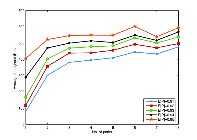
Figure 2.3: Simulation results: Average throughput vs. no. of paths for multiple path TCP-RLC connection. Note that the throughput of $M$ separate traditional TCP connections (whether over wired or wireless downlink networks) does not increase with the number of paths. In addition, TCP throughput over wireless downlink network with fixed FEC coding rate is $\Theta(1)$. Thus, the throughput of the traditional TCP over wireless downlink network where the channel fluctuation changes at the time scale of the RTT is low and does not increase with the number of paths.

The average throughputs we obtained are shown in Figure 2.3 as a function of the number of paths. As the number of paths increases, the average throughput increases towards $\mathbb{E}\left[P\right]CM$ ($CM$ is fixed) in a concave manner, indicating that going from one path to two paths gives much gain in throughput, especially when $p_{\min}$ is small. The throughput should reach 700Kbps (for $\mathbb{E}\left[P\right]=0.91$) to 730Kbps (for $\mathbb{E}\left[P\right]=0.95$).

2.5 Appendix

2.5.1 TCP-RLC Protocol

In this subsection, we give a brief description of NS-2 simulation implementation details. We break the description of TCP-RLC into three subsections.

Source Architecture

ACK and pseudo ACK

TCP-RLC uses two types of ACK’s: ACK, as used in the plain TCP and pseudo ACK, which we describe here.

Plain ACK’s cumulatively acknowledge the reception of all packets with frame numbers smaller than or equal to the ACK.

In our context, a lost data packet can be “made up” by a future coded packet, and we would like the sliding congestion window to slide forward and have delay-bandwidth product worth of packets in transit. Thus, we use a strategy similar to that in [71], where degrees of freedom are ACKed. In our context, we refer to this as a pseudo ACK, which simply ACKs any out of order data packet or coded packet that helps in decoding the smallest-index missing packet (e.g., if the sink has received packets 1, 2, 3, and 7, the smallest-index missing packet is 4). Note that with regular TCP, out-of-order packets would trigger duplicates ACK’s that would lead to a loss of throughput.

To summarize: ACK – cumulatively acknowledges in-order packet arrivals; pseudo ACK – acknowledges out-of-order data packet/coded packet arrivals that help in decoding the missing packets.

Sliding congestion window

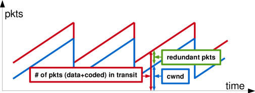
Figure 2.4: Evolution of congestion window: the total number of packets in transit is composed of cwnd high priority packets (data packets) + redundant packets (RLC encoded packets). The number of redundant packet is some multiple of cwnd, and has to be greater than $p_{1}$. Note that without priority transmission at the wireless router, this will reduce the throughput.

The source maintains a congestion window $W$, which is the same as the size of the coding block for TCP-RLC. All packets transmitted are marked either high or low priority; the source allows only $W$ high priority packets to be in transit. Each time a high priority packet is transmitted, it transmits $r$ low priority packets as well, where $r\geq 1/p_{\min}-1$.

The source maintains variables, last-ACK and SN. All packets with frame numbers lower than last-ACK are assumed to have been successfully received. SN is the frame number of the starting packet in the coding block currently being transmitted. If pseudo ACK or ACK arrives “acknowledging” the reception of SN, a new coding block is encoded and readied for transmission, with the coding block size being $W+1$ packets. This is because acknowledgment of packet number SN implies a RTT has been elapsed, which is enough time for $W$ packets to have been successfully received and decoded by the sink.

Multiple paths

When multiple paths are used, the marking of packets is done by the paths independently. Each path is maintained by a path controller and the controller maintains a congestion window, $cwnd_{i}$; another top-level controller maintains $cwnd$, which is used as the size of the coding block. After the packets are encoded, they are passed to path controllers (thus, coded packets are “mixed” across paths, which in-turn leads to statistical multiplexing across paths). Each path marks packets either high or low priority. In each RTT slot, the number of high priority packets in transit is equal to $cwnd_{i}$. The number of low priority packets (coded packets) per path is equal to $r\times cwnd_{i}.$ Each packet going out on a path contains the block number and block size, which is also equal to $cwnd_{i}$. In each RTT slot, if the sink on path $i$ receives $cwnd_{i}$ packets (either high or low priority), $cwnd_{i}$ increases by one; else $cwnd_{i}$ reduces by half. Note that single path is just a special case of multiple paths; and the variables $cwnd$ and $cwnd_{1}$ are the same. (In the single-path case, the role played by the separate path controllers is subsumed into the source controller.)

There are two levels of ACK’s; one level for source controller (source level ACK, consisting of ACK and p-ACK) and the other for path controllers (path level ACK). Note that: (i) path level ACK is a new ACK introduced for multi-path TCP – there is no equivalent in the single-path case, and (ii) the three types of ACKs described here is abstracted into a single indicator function for success/drop in the analysis (see eq. (2.2) in section 2.2). Source controller level ACK’s affect $cwnd$ and moves the coding window; path controller level ACK’s affect $cwnd_{i}$’s and moves the block numbers.

Destination Architecture

Upon reception of a packet, the destination examines if it is the next expected (i.e., smallest-index missing) packet. If it is, the destination sends an ACK cumulatively acknowledging all packets upto and including the just received packet. If not, the destination sees if the packet is an innovative packet that can be used to decode the next expected. (A packet is innovative if it is linearly independent of all packets received so far, i.e. it can help in decoding the next expected packet. For a complete definition of innovative packets, see [46] and [29].) In case the packet is helpful, the destination sends a pseudo ACK with next expected packet number + total number of innovative packets accumulated that can help in decoding the next expected packet. If the packet does not help in decoding the next expected packet, the destination sends a duplicate ACK.

Wireless Router Architecture

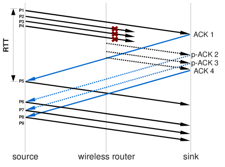
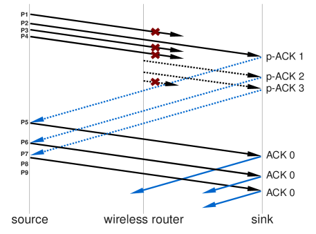
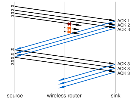
Figure 2.5: Illustrative example

As mentioned, the wireless router maintains two buffers for each flow. A FIFO buffer is maintained for high priority packets; a LIFO buffer is maintained for low priority packets. The FIFO buffer does not need to be large, but large enough to handle packet processing execution. The LIFO buffer needs to be large enough to handle RTT worth of packets. In our implementation, we do not have an explicit AQM mechanism at the router (other than tail-drop); however, even without AQM we observe large performance gains through simulations.

Illustrative Example

We illustrate the additive increase, multiplicative decrease component of TCP-RLC and the pseudo ACK’s using three examples. The examples are for when a TCP connection uses a single path, and the data and coded packets are marked high and low priority, respectively. Although the TCP source uses retransmission time-outs for when there is no response from the sink for long period of time, we do not show this in our examples.

1. Additive increase: When there is no congestion at the wireless router and the sink receives enough data and coded packets in a coding block, the sink will be able to recover any missing data packets. In Figure 2.5, the four packets P1-P4 are encoded together. While P1 is successfully received by the sink, P2-P4 are dropped/lost due to bad wireless channel. However, the sink has received enough coded packets to recover packet P2-P4. As the sink receives these coded packets, it sends out a pseudo ACK for each one. This enables the source to move the congestion window forward, keeping the “pipe” between the source and the sink full. When the sink recover P2-P4, it sends out an ACK acknowledging the successful reception of packets upto P4. Note that the congestion window is increased by one packet, and thus new packets P5-P9 are encoded together.

2. Multiplicative decrease (bad wireless channel): When too many packets that belong in the same coding block are dropped due to bad wireless channel, duplicate ACK’s will be triggered when packets that do not help in decoding the next expected packet. In Figure 2.5, data packet P1, P3 and P4 are dropped and not enough coded packets arrive due to bad wireless channel. When packets P5-P7 arrive at the sink, duplicate ACK’s are sent out and the source will cut the congestion window. Note that when p-ACK 1 is received by the source, a new coding block P5-P9 is encoded and passed to path controllers. However, when the duplicate ACK’s are received, the source decreases the congestion window by half to two packets, and restarts transmission starting from P1.

3. Multiplicative decrease (congestion at wireless router): Where there is a congestion at the wireless router, the router will be busy transmitting data (high priority) packets, and no or very few coded (low priority) packets will be transmitted. In Figure 2.5, packet P1-P3 are successfully received, but no coded packets are received to help the sink recover the packet P4, which has been lost due to then bad wireless channel condition. Thus, the sink will send out duplicate ACK’s and the source will cut the congestion window and restart transmission starting from P4.

Chapter 3 Time-Scale Decoupled Routing and Rate Control in Intermittently Connected Networks

3.1 Introduction

There recently has been much interest in intermittently connected networks (ICNs). Practical use of such networks include military scenarios in which geographically separated clusters of soldiers are deployed in a battlefield. Each cluster is connected wirelessly internally, but the clusters of soldiers rely on unmanned aerial vehicles to transport battlefield information between clusters. In such a case, building a communication network can take too much time as these combat units must be deployed rapidly, and wireless connections are often susceptible to enemy jamming or the communication/RF ranges might not be large enough.

Another scenario of interest is a sensor network composed of multiple clusters, with each cluster containing low power sensor nodes. The data collected by the sensor nodes must either be transmitted to a data fusion node or to another cluster. To do this, the sensor nodes rely on mobile nodes that provide inter-cluster connectivity; thus resulting in a network with multiple time-scales and intermittent connectivity.

In this dissertation, we consider a network of clusters of nodes connected via “mobile” nodes (see Figure 3.1 for an example). Internally, each cluster has many nodes connected via a (multi-hop) wireless network. Each cluster has at least one gateway node. (We will call the other nodes in the cluster internal nodes.) These gateways are the designated representatives of the clusters, and they are the only ones able to communicate with the mobiles – traffic from one cluster to another cluster (inter-cluster traffic) must be funneled through the gateways, both in the source cluster and in the destination cluster. The mobiles and gateways exchange packets (pick-ups and drop-offs) on contact. Each contact is made over a high capacity link and is long enough for a large quantity of data to be exchanged. The mobiles then move between clusters, and on contact with a gateway in the destination cluster, packet drop-offs are made.

A key challenge in the network above is the fact that intermittently connected networks have several time-scales of link variability. For instance, wireless communication between soldiers within the same cluster is likely to occur at a time-scale several orders of magnitude faster than communication across clusters (which needs to use the mobile carriers). In this context, there are essentially two time-scales: (a) within a cluster, where wireless links are formed in an order of tens of milliseconds, and (b) across clusters where the time-scale could be tens of seconds, to minutes. To communicate from one node to another node in the same cluster poses no significant problem – one can use existing protocols such as TCP. However, for two nodes in two different clusters to communicate, they must use the mobile nodes, as these mobiles move between clusters to physically transport data. Hence, the mobile communication time scale is many, many times greater than the electronic communication time scale. Any communication protocol that relies on fast feed-back (in the order of milliseconds to tens/hundreds of milliseconds) incurs severe performance degradation. The mobiles may be able to transport a large quantity of data (of the order of mega or giga bytes) in one “move,” but to move from one cluster in one part of a network to another part still takes time (of the order of seconds to minutes).

The design and development of communication protocols for intermittently connected networks, therefore, must start with an algorithm with as few assumptions about the underlying network structure as possible. The back-pressure (BP) routing algorithm [73] was introduced nearly two decades ago by Tassiulas and Ephremides with only modest assumptions about the stability of links, their “anytime” availability, or feasibility of fast feed-back mechanism; yet remarkably, it is throughput optimal (throughput performance achieved using any other routing algorithm can be obtained using the back-pressure algorithm [73]) as well as resilient to changes in the network. The BP routing algorithm is a dynamic routing and scheduling algorithm for queuing networks based on congestion gradients. The congestion gradients are computed using the differences in queue lengths at neighboring nodes (the routing part). Then, the back-pressure algorithm activates the links so as to maximize the sum link weights of the activated links, where the link weights are set to the congestion gradient (the scheduling part). Over the years, there has been continued effort to further develop back-pressure type algorithms to include congestion control and to deal with state-space explosion and delay characteristics [48, 68, 23, 50, 2, 82, 81, 47, 78, 3].

However, the traditional back-pressure algorithm is impractical in intermittently connected networks, even though it is throughput optimal. This is because the delay performance and the buffer requirement of the back-pressure algorithm in the heterogeneous connectivity setting of the ICNs increase with the product of the network size and the time scale of the intermittent connections – i.e., the larger the network or more intermittent and sporadic the connections, the larger the delay and buffer requirement. However, we believe that the back-pressure algorithm is a reasonable starting point for developing rate control/routing protocols for intermittently connected networks. In this dissertation, we design, implement and evaluate the performance of two-scale back-pressure algorithms specially tailored for ICNs.

3.2 Related Works

The back-pressure algorithm and distributed contention resolution mechanism in wireless networks, in one form or another, have been studied and implemented in [78, 55, 47, 67, 41, 4, 56, 34]. [78] improves TCP performance over a wireless ad-hoc network by utilizing the back-pressure scheduling algorithm with a backlog-based contention resolution algorithm. [55] improves multi-path TCP performance by taking advantage of the dynamic and resilient route discovery algorithmic nature of BP. The authors in [47] have implemented and studied back-pressure routing over a wireless sensor network. They have used the utility-based framework of the traditional BP algorithm, and have developed implementations with good routing performance for data gathering (rate control is not studied in [47]). Their chief objective is to deal with the poor delay performance of BP. [67] is an implementational study of how the performance of BP is affected by network conditions, such as the number of active flows, and under what scenarios backlog-based contention resolution algorithm is not necessary. [41] studies utility maximization with queue-length based throughput optimal CSMA for single-hop flows (with no routing or intermittent connectivity). More recent works on contention resolution mechanism are [4, 56, 34]. In [4], a queue-based contention resolution scheme is proposed; however, the proposed algorithm only uses the local estimates of the neighbors’ queue lengths to change the contention window parameter of IEEE 802.11, unlike the original back-pressure algorithm which requires explicit neighborhood queue length feedback. The authors of [56] proposed another form of queue-based contention resolution algorithm, which they conjecture does not require any neighborhood queue length feedback or message passing; however, the algorithm in [56] requires larger buffers, resulting in long delays. Channel access mechanism not based on queue lengths is proposed in [34]. Here, the authors propose a distributed time-sharing algorithm that allocates time slots based on the number of flows in the wireless network. Lastly, [2] is not an implementation, but discusses a lot of issues related to BP routing with rate control implementation. Our study differs from all of them in that we focus on the multiple time-scales issue in an intermittently connected network (thus, queues throughout the network get “poisoned” with the traditional BP), and study modifications that loosely decouple the time-scales for efficient rate control.

A cluster-based back-pressure algorithm has been first studied in [82] to reduce the number of queues in the context of traditional networks. However, the algorithm as proposed in [82] in general does not separate between the fast intra-cluster time scale and the slow inter-cluster timescales due to intermittently connected mobile carriers, thus leading to potentially large queue lengths at all nodes along a path. (We will demonstrate this in Section 3.3.) Our proposed algorithms in this dissertation explicitly decouples the two time scales by separating the network into two layers, with each layer operating its own back-pressure algorithm, and by allowing the two layers to interact in a controlled way at nodes that participate in inter-cluster traffic. This explicit separation is the key property that leads to much smaller buffer usage and end-to-end delays and more efficient network resource utilization.

Initially, the approach taken in intermittently connected networks and DTNs for routing was based on packet replications. The simplest way to make sure packets are delivered is to flood the “mobile” portion of the network so that the likelihood of a packet reaching the destination increases as more and more replicas are made [77]. A more refined approach is to control the number of replicas of a packet so that there is a balance between increasing the likelihood and still leaving some capacity for new packets to be injected into the network [8, 66, 15, 77, 43]. Another refined approach is to learn the intermittently connected topology and use this knowledge to route/replicate through the “best” contacts and encounters and avoid congestion [33, 35, 64, 74, 42].

[51, 79, 27] study networks that are closer to ours. In [79], distant groups of nodes are connected via mobiles, much like our network but with general random mobility. At the intra-group level, a MANET routing protocol is used for route discovery, and at the inter-group level, the Spray-and-Wait algorithm [66] is used among mobiles to decrease forwarding time and increase delivery probability. [51] augments AODV with DTN routing to discover routes and whether those routes support DTN routing and to what extent they support end-to-end IP routing and hop-by-hop DTN routing. [27] studies how two properties of the mobile nodes, namely whether a mobile is dedicated to serve a specific region (ownership) and whether the mobile movement can be scheduled and controlled by regions (scheduling time), affect performance metrics such as delay and efficiency.

Because replication-based algorithms inject multiple copies of a packet, they suffer from throughput drops. However, all the aforementioned replication-based algorithms are valuable as they provide insight into engineering an efficient and robust ICN protocol. There is (to the best of our knowledge) no literature on rate control over ICNs. We demonstrate in this dissertation that it is possible to obtain utility maximizing rate allocation, even though there is the “mobile-gateway” time scale that operates much slower than the wireless communication time scale, and all inter-cluster packets have to pass through the two different time scales.

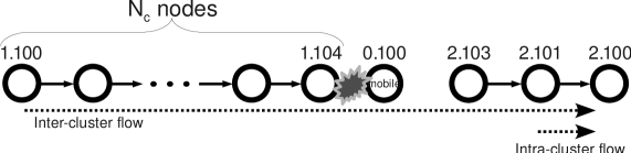
Figure 3.1: Our ICN consists of two clusters and one mobile node connecting these clusters. We have one intra-cluster flow from 2.101 to 2.100, and one inter-cluster from flow 1.100 to 2.100, which must rely on the mobile to transport data from the left to the right cluster.

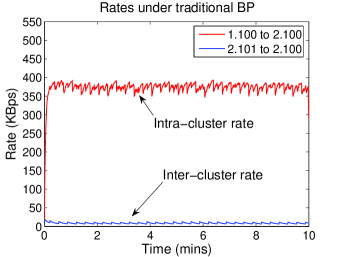
(a) Inter-cluster and intra-cluster rates

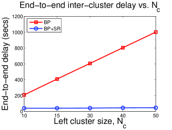
(b) End-to-end delay as a function of $N_{c}$

Figure 3.2: The inter-cluster rate suffers serious throughput degradation under the traditional BP with rate controller because the inter-cluster source mistakenly sees the intermittent link as a low-capacity (with low delay) link and not as a high-capacity (with high delay) link (see Figure 3.2(a)). Under the traditional BP, even if the inter-cluster rate is fixed to the correct value, the inter-cluster end-to-end delay grow to be extremely large as the source cluster size increases (see Figure 3.2(b)).

3.3 Motivation: Difficulties with Traditional Back-Pressure

Consider a simple, intermittently connected line network as shown in Figure 3.1. We have two clusters geographically separated. We have two gateways (1.104 and 2.103) representing the left and right clusters, respectively. In the left cluster, we have $N_{c}$ nodes, and in the right cluster, we have three nodes. Between these two clusters, we have a “mobile” contact node 0.100 that moves from one cluster to the other every ten seconds. On contact, the mobile and the gateways (the designated nodes in the cluster that can communicate with the mobiles) can exchange a large quantity of packets. Finally, there are two flows; an inter-cluster flow originating from 1.100 and an intra-cluster flow originating from 2.101; both flows are destined for 2.100.

In this network, routing is straightforward. But the question here is: What is the rate at which these flows can transmit data? An even more basic question is: Can these flows attain high and sustainable throughput, provided that the link capacity between the mobiles and gateways is high enough (albeit with extreme delays)? How close can we get to the maximum throughput allowed by the network? Can we obtain utility-maximizing rate allocation over an ICN? What will be the delay performance in such networks?

The answer to this is clearly negative, if TCP is used for rate control, and we shall see that even with traditional back-pressure algorithms [73, 23] that have a theoretical guarantee that the above is possible, in a practical setting, the answer still seems to be negative!

To put the above statement in context, we know that the back-pressure (BP) routing/rate control algorithm is throughput optimal [73], meaning that if any routing/rate control algorithm can give us certain throughput performance, so can the back-pressure algorithm. Contra-positively, if the back-pressure algorithm cannot give a certain throughput performance, no other algorithm can do so. Further, a rate controller based on utility maximization can be added to this framework [68, 23, 50] that is theoretically utility maximizing, and it chooses rates that (averaged over a long time-scale) lead to high and sustainable throughput corresponding to the rates determined via an optimization problem [68, 23, 50].

We first consider the performance of a traditional BP based routing/rate control algorithm. In Figure 3.2(a), we plot the rate trace of the two (inter- and intra-cluster) flows (with $N_{c}=2$). (Figure 3.2(a) is obtained experimentally. Each source uses the BP congestion algorithm [48, 68, 23, 50] which we will describe later). In the figure, we can see that the inter-cluster traffic performs very poorly, even though the mobile-gateway contact has enough capacity. The reason is simple – the BP congestion control uses the local queue length as a congestion signal, and between two successive contacts that can be seconds or minutes apart, there is a large queue build-up to the point that the inter-cluster source mistakenly believes that the network has low-capacity (and low-delay) links. Because of this, the inter-cluster source is not able to fully utilize the contacts (see Figure 3.2(a)).

Importantly, this rate achieved by the inter-cluster traffic is much lower than that predicted by the theory (the theory predicts that intra-cluster rate is $\approx$ 200KBps, and the inter-cluster rate $\approx$ 100KBps). This is because the theoretical results hold only when the utilities of users are scaled down by a large constant – this is to (intuitively) enable all queues in the network to build up to a large enough value in order to “dilute” the effects of the “burstiness” of the intermittently connected link. However, scaling down the utilities by a large constant will result in long queues over the entire network, even at nodes that do not participate in inter-cluster traffic.

Furthermore, even if the inter-cluster source is aware of the presence of these intermittent mobile-gateway links and therefore can transmit at the correct rate (i.e., a genie computes the rate and tells this to the source), the problem can manifest itself in another way.

Consider the same network as in Figure 3.1, but we just have the inter-cluster flow from 1.100 to 2.100; however, we vary the left cluster size $N_{c}$ from 10 to 50. See Figure 3.2(b). (Figure 3.2(b) is obtained from simulations.) We run the traditional BP algorithm (with no rate controller, as the genie has solved this problem) and fix the source rate at 200KBps. In this case, there is large backlog that builds up not only at node 1.104 (the intermittently connected gateway), but also at every node in the left cluster.

3.3.1 Main Contributions

In this chapter, we design, implement and empirically study the performance of a modified back-pressure algorithm that has been coupled with a utility based rate controller for an intermittently connected network. Our contributions are:

1. We present a modified back-pressure routing algorithm that can separate the two time scales of ICNs. Separating the time scales improves the end-to-end delay performance and provides a throughput arbitrarily close to the theory. A key advantage of this modified BP algorithm is that it maintains large queues only at nodes which are intermittently connected; at all other nodes, the queue sizes remain small.

2. On top of our modified back-pressure routing algorithm, we implement a rate control on our testbed. The essential components of our testbed are built with modified MadWifi and Click [39]. The nodes in our testbed are organized into multiple clusters, with intermittent connectivity emulated using an Ethernet switch.

3. Using this testbed, we first show that the traditional back-pressure algorithms coupled with a utility function-based rate controller is not suitable for intermittently connected networks, and leads to a large divergence between theoretically predicted rates and actual measurements (shown for an intermittently connected line network). We then present measurement results using our time scale decoupled algorithm on a line network and on a larger sized network.

4. Finally, we present a practical implementation of shadow queues developed by the authors in [14]. Using our implementation, we demonstrate there is a nice trade-off between shorter end-to-end inter-cluster delay and the network capacity utilization.

3.4 Network Model

The time is slotted, with $t$ denoting the $t^{\text{th}}$ time slot. The intermittently connected network consists of multiple clusters. Each cluster $\mathcal{C}_{i}$ is represented by a graph $\mathcal{G}_{\mathcal{C}_{i}}=(\mathcal{N}_{\mathcal{C}_{i}},\mathcal{L}_{\mathcal{C}_{i}}),$ where $\mathcal{N}_{\mathcal{C}_{i}}$ is the set of nodes in $\mathcal{C}_{i}$ and $\mathcal{L}_{\mathcal{C}_{i}}$ is the set of links. Let $\mathcal{C}(n)$ denote the cluster to which node $n$ belongs. The clusters are geographically separated, and two nodes in distinct clusters cannot communicate with each other directly (they must rely on the mobiles to transport data).

The clusters are connected by a set $\mathcal{M}$ of mobile carrier nodes that move around to carry packets from one cluster to another. For each cluster, the set of nodes that can communicate with the mobiles is fixed. These nodes are named as gateways; those nodes that cannot communicate with the mobiles directly are called internal nodes. Let $\mathcal{I}_{\mathcal{C}_{i}}$ and $\mathcal{H}_{\mathcal{C}_{i}}$ denote the set of internal nodes and gateways in $\mathcal{C}_{i}$, respectively.

We use $g(i,j)$ to denote gateway $j$ in cluster $\mathcal{C}_{i}$. To simplify the notations, we assume that gateways $g(\cdot,j)$ have access to mobile $m(j)$ only. The mobiles change gateways every $T$ time slots, which is called a super time slot. We let $\tau$ denote the $\tau^{\text{th}}$ super time slot. Here, $T$ is a very large number. A time slot is the time scale of one intra-cluster packet transmission, and $T$ is the time scale of the mobility (thus, a time slot is roughly a few milliseconds long, and $T$ is roughly $>10^{3}$ to reflect the mobility time scale which is seconds or minutes long). In our model, the size of the clusters is $<<T$.

We assume that the mobility of the mobiles follows a Markov process. Given that mobile $m(j)$ is at gateway $g(i_{1},j)$ at the beginning of super time slot $\tau,$ the probability that it moves to gateway $g(i_{2},j)$ at the beginning of the super time slot $\tau+1$ is

$$\mathbb{P}\left(m(j)-g(i_{2},j)\text{ in }\tau+1|m(j)-g(i_{1},j)\text{ in }\tau\right)$$

$$=\mathbf{P}_{m(j)}(i_{1},i_{2})$$

where “$-$” means that the mobile and the gateway are in contact. Let $\mathbf{P}_{m(j)}$ denote the transition probability matrix of mobile $m(j)$ and let $\pi_{m(j)}$ be the corresponding stationary distribution. The Markov chains are assumed to be aperiodic and irreducible. The assumption that $g(\cdot,j)$ only have access to $m(j)$ is not necessary; we make this assumption to simplify our notations.

3.4.1 Traffic Model

A traffic flow is defined by its source and destination. We assume that the sources and destinations are all internal nodes. If the source and the destination lie in the same cluster, then the traffic flow is an intra-cluster traffic, and the intra-cluster traffic can be routed only within the cluster. If the source and the destination lie in different clusters, the traffic flow is an inter-cluster traffic. We let $[s,d]$ denote the flow from $s$ to $d,$ $\mathcal{F}$ denote the set of all flows, and $\mathcal{F}_{\text{inter}}$ and $\mathcal{F}_{\text{intra}}$ be the sets of all inter- and intra-cluster flows, respectively. We let $x_{s}^{d}$ be the number of packets source $s$ generates per time slot for destination $d$, $\textbf{x}=\{x_{s}^{d}:[s,d]\in\mathcal{F}\},$ and $\textbf{x}_{\text{intra}(\mathcal{C})}$ be the set of intra-cluster traffic rates in cluster $\mathcal{C}$.

Note that all inter-cluster traffic flows must be forwarded to the gateways in source clusters, then carried over to the gateways in destination clusters via the mobile nodes before reaching their destinations.

3.4.2 Communication Model

Let $\mu_{(n_{1},n_{2})}[t]$ denote the transmission rate (packets/time slot) of link $(n_{1},n_{2})$ at time $t,$ and $\vec{\mu}_{\mathcal{C}_{i}}[t]=\{\mu_{(n_{1},n_{2})}[t],~{}(n_{1},n_{2})\in\mathcal{L}_{\mathcal{C}_{i}}\}$. Let $\Gamma_{\mathcal{C}_{i}}$ be the convex hull of the set of all feasible transmission rates in cluster $\mathcal{C}_{i}$. We note that in general, $\vec{\mu}_{\mathcal{C}_{i}}[t]$ and $\Gamma_{\mathcal{C}_{i}}$ depend on the interference model used for cluster $\mathcal{C}_{i}$.

We assume that a mobile and a gateway can send $R$ packets to each other per contact. We assume that the transmissions between mobiles and gateways do not cause interference to other transmissions.

For an example, see the network depicted in Figure 3.4. Here, we have three clusters, with two gateways in each and each cluster connected in a grid. We have pairs of nodes in different clusters communicating using the two mobiles (inter-cluster flows), which shuffle between these clusters transporting data from one cluster to another. In addition, we have intra-cluster flows in each cluster.

3.5 Two-Scale BP with Queue Reduction: BP+SR

In this section, we introduce our two-scale back-pressure routing algorithm (which we refer to as BP+SR (Source Routing)) that separates the times scales of inter-cluster and intra-cluster connections, while at the same time, reducing the number of queues that need to be maintained. We build on this two-scale back-pressure algorithm in section 3.6 to implement a utility-maximizing rate controller.

3.5.1 Queuing Architecture

In our algorithm, the network maintains two types of queues. The first type, referred to as type-I, will be denoted by $q$, and the second type, type-II, will be denoted by $u$.

Any internal node $n_{1}$ maintains a type-II queue $u_{n_{1}}^{g}$ for each gateway $g$ in the same cluster and a type-I queue $q_{n_{1}}^{n_{2}}$ for each node $n_{2}$ in the same cluster. A gateway $g_{1}$ maintains a type-II queue $u_{g_{1}}^{g_{2}}$ for each of other gateways $g_{2}$ in the network (even for gateways in the same cluster).

For each node $n$ in the same cluster, gateway $g$ maintains both a type-I queue and a type-II queue for node $n$. A mobile $m$ maintains a separate type-II queue $u_{m}^{g}$ for each gateway $g$ in the network. We use $q_{a}^{b}[t]$ ($u_{a}^{b}[\tau]$) to denote the length of the type-I (type-II) queue maintained by node $a$ for node $b$ at the beginning of the time slot $t$ (super time slot $\tau$). Note that $u_{n}^{n}=0$ and $q_{n}^{n}=0$ at all times $\forall~{}n$.

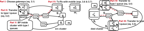
Figure 3.3: In this figure, we break down the BP+SR algorithm into six parts. Part I is the source routing. Parts V and VI are the intra- and inter-cluster back-pressure routing algorithms, respectively. The two back-pressure algorithms interact via packet transfers between type I and II queues. Part III is for the load balancing over different gateways in the same cluster using the intra-cluster back-pressure, i.e., the gateways use the intra-cluster back-pressure as the back haul link for transferring packets between them.

3.5.2 BP+SR Algorithm

We now present our two-scale BP routing algorithm, BP+SR (Source Routing). We give a high-level highlight using Figure 3.3 before discussing the algorithm in details. First, an inter-cluster traffic source takes a group of packets and chooses the optimal gateways (in both source and destination clusters) through which these packets should be routed (Part I). The optimal gateways chosen can change over time. These packets are routed from the source to the chosen optimal source gateway, and from the chosen optimal destination gateway to the destination using the intra-cluster back-pressure inside the respective clusters (Part V); they are routed from the source gateway to the destination gateway using the inter-cluster back-pressure (Parts III and VI). The interaction between the two back-pressure routing algorithms happens through packets transfers between the two types of queues (Parts II, III, and IV). Part VII is presented for mathematical convenience and is not in the actual protocol.

Part I: Selecting source and destination gateways

At the beginning of super time slot $\tau$, the inter-cluster traffic source $s$ picks the source and destination gateways $g_{s}^{*}[\tau]$ and $g_{d}^{*}[\tau]$ such that

$$\left(g_{s}^{*}[\tau],g_{d}^{*}[\tau]\right)\in\arg\min_{\begin{subarray}{c}g_{s}\in\mathcal{H}_{\mathcal{C}(s)}\\ g_{d}\in\mathcal{H}_{\mathcal{C}(d)}\end{subarray}}\left(u_{s}^{g_{s}}[\tau]+u_{g_{s}}^{g_{d}}[\tau]+u_{g_{d}}^{d}[\tau]\right).$$ (3.1)

This route selection is done at the beginning of each super time slot (i.e., every $T$ time slots). The source $s$ makes the routing decision (Eq. 3.1) independently of other inter- and intra-cluster sources. The source and destination gateways are chosen such that the pair minimizes the total queue lengths considering the intra-cluster path from the source to its gateway, the inter-cluster path between the two gateways, and the intra-cluster path between the destination gateway and the destination node.

Part II: Traffic control at the source nodes

• For an inter-cluster flow $[s,d],$ the source node $s$ deposits newly arrived packets into queue $u_{s}^{g_{s}^{*}[\tau]}$ during time slot $t\in[\tau T,(\tau+1)T).$ The identities of the source gateway $g_{s}^{*}[\tau]$ and the destination gateway $g_{d}^{*}[\tau]$ are recorded in the headers of the packets.

• For an intra-cluster flow $[s,d],$ the source node $s$ deposits the new arrived packets into queue $q_{{s}}^{{d}}.$

• Define $\theta_{s}^{g_{s}}[\tau]=u_{s}^{g_{s}}[\tau]/K_{s},$ where $K_{s}=T/|{\cal C}(s)|.$ ($|\mathcal{C}|$ is the number of nodes in cluster $\mathcal{C}$.) Consider the queues associated with gateway $g_{s}\in\mathcal{H}_{\mathcal{C}(s)}.$ If

  $$\theta_{s}^{g_{s}}[\tau]>q_{s}^{g_{s}}[t]$$ (3.2)

  at time $t\in[\tau T,(\tau+1)T),$ $\eta$ packets are transferred from queue $u_{s}^{g_{s}}$ to queue $q_{s}^{g_{s}}$ at the beginning of time slot $t$. ($\eta$ is some positive value greater than the largest transmission rate out of any node inside a cluster.)

  When a packet arrives at the source gateway $g_{s}^{*}$, the source gateway would set the next destination of that packet to $g_{d}^{*}$, which it would find in the packet header. (See Eq. (3.1).) The gateway would then insert that packet into the queue $u_{g_{s}^{*}}^{g_{d}^{*}}$.

To achieve throughput optimality, an inter-cluster traffic source must do source routing as in Eq. (3.1), and when it does source routing, the length of the queue $u_{s}^{g_{s}}$ will become of order $\Theta(T)$, and there must be a way to release the packets stored in the queue $u_{s}^{g_{s}}$ into the cluster so they can reach the source gateway. The purpose of Eq. (3.2) is exactly that – to release/transfer the packets from $u_{s}^{g_{s}}$ (type-I queue) to $q_{s}^{g_{s}}$ (type-II queue) at a controlled and acceptable rate to the cluster. The factor $|\mathcal{C}(s)|$ is needed so as to prevent the inter-cluster end-to-end delay from scaling with the cluster size.

Part III: Traffic control at the gateway nodes

The gateway $g_{1}$ computes $l_{g_{1},g_{2}}[\tau]\in\operatorname*{arg\,max}_{l\in\left(\bigcup_{\mathcal{C}}\mathcal{H}_{\mathcal{C}}\right)}(u_{g_{1}}^{l}[\tau]-u_{g_{2}}^{l}[\tau])$ at the beginning of each super time slot for each gateway $g_{2}$ in the same cluster. Define $\theta_{g_{1}}^{g_{2}}[\tau]=\left\{u_{g_{1}}^{l_{g_{1},g_{2}}[\tau]}[\tau]-u_{g_{2}}^{l_{g_{1},g_{2}}[\tau]}[\tau]\right\}/K_{g_{1}}$ where $K_{g_{1}}=T/|\mathcal{C}(g_{1})|$. At each time slot $t\in[\tau T,(\tau+1)T)$, $g_{1}$ transfers $\eta$ packets from $u_{g_{1}}^{l_{g_{1},g_{2}}[\tau]}$ to $q_{g_{1}}^{g_{2}}$ if

$$\theta_{g_{1}}^{g_{2}}[\tau]>q_{g_{1}}^{g_{2}}[t].$$ (3.3)

The next destination of the transferred packets is temporarily set to $g_{2}$; when $g_{2}$ receives those packets, they are inserted into $u_{g_{2}}^{g_{d}^{*}}$, where $g_{d}^{*}$ (from Eq. (3.1)) can be found in the packet headers.

Part III is used by the gateways (that are in the same cluster) to balance the load amongst themselves using the intra-cluster resources. That is, the gateways can us any available bandwidth in the cluster to shift load from one gateway to another.

Part IV: Traffic control at the destination gateways

When the packets arrive at their destination gateways, they are deposited into queue $u_{g_{d}}^{d}$. Let $\theta_{g_{d}}^{d}[\tau]=u_{g_{d}}^{d}[\tau]/K_{g_{d}}$, where $K_{g_{d}}=T/|\mathcal{C}(g_{d})|$. In each time slot $t\in[\tau T,(\tau+1)T)$, $\eta$ packets are transferred from $u_{g_{d}}^{d}$ to $q_{g_{d}}^{d}$ if

$$\theta_{g_{d}}^{d}[\tau]>q_{g_{d}}^{d}[t].$$ (3.4)

Part V: Routing and scheduling within a cluster

In each time slot $t$, each cluster $\mathcal{C}$ computes $\vec{\mu}_{\mathcal{C}}[t]$ such that

$$\vec{\mu}_{\mathcal{C}}[t]=\operatorname*{arg\,max}_{\vec{\mu}\in\Gamma_{\mathcal{C}}}\left\{\sum_{(m,n)\in\mathcal{L}_{\mathcal{C}}}\mu_{(m,n)}P_{(m,n)}[t]\right\}$$ (3.5)

where $P_{(m,n)}[t]=q_{m}^{j_{(m,n)}[t]}[t]-q_{n}^{j_{(m,n)}[t]}[t]$ and $j_{(m,n)}[t]=\operatorname*{arg\,max}_{j}\left\{q_{m}^{j}[t]-q_{n}^{j}[t]\right\}$. After the computation, node $m$ transmits $\mu_{(m,n)}[t]$ packets out of queue $j_{(m,n)}[t]$ to node $n$ in time slot $t$. $\Gamma_{\mathcal{C}}$ is the set of all feasible rate in the cluster $\mathcal{C}$.

Part VI: Routing between gateways and mobiles

At the beginning of each super time slot $\tau$, the mobile $m$ and the gateway $g$ that are in contact compute the following:

$$j_{(m,g)}[\tau]=\operatorname*{arg\,max}_{j\text{ gateway }}\left\{u_{m}^{j}[\tau]-u_{g}^{j}[\tau]\right\},$$ (3.6)

$$j_{(g,m)}[\tau]=\operatorname*{arg\,max}_{j\text{ gateway}}\left\{u_{g}^{j}[\tau]-u_{m}^{j}[\tau]\right\}.$$ (3.7)

Afterwards, $m$ transmits $R$ packets from the queue $u_{m}^{j_{(m,g)}[\tau]}$ to $g$, and the gateway $g$ transmits $R$ packets from the queue $u_{g}^{j_{(g,m)}[\tau]}$ to $m$, maximizing $R\left(P_{(m,g)}[\tau]+P_{(g,m)}[\tau]\right)$.

Part VII: Real and regulated queues

For analytical purposes, we assume that each type-II queue at a gateway consists of two parts: a real type-II queue, denoted $\tilde{u}$, and a regulated type-II queue, denoted $u$. At gateway $g_{1}$, the amount of packets transferred from the real queue $\tilde{u}_{g_{1}}^{g_{2}}$ to the regulated queue $u_{g_{1}}^{g_{2}}$ in time slot $t$ is $y_{g_{1}}^{g_{2}}[t]=(1+\delta)\sum_{[s,d]\in\mathcal{F}_{\text{inter}},~{}s\in\mathcal{I}_{\mathcal{C}(g_{1})}}x_{s,g_{1}}^{g_{2},d}[t]$ where $g_{2}$ is another gateway, and the amount of packets transferred from $\tilde{u}_{g_{1}}^{d}$ to $u_{g_{1}}^{d}$ is $y_{g_{1}}^{d}[t]=(1+\delta)\sum_{[s,d]\in\mathcal{F}_{\text{inter}},~{}d\in\mathcal{I}_{\mathcal{C}(g_{1})}}x_{s,g_{2}}^{g_{1},d}[t]$ where $d$ is an internal node in $\mathcal{C}(g_{1})$ and $\delta>0$, and

$$x_{s,g_{s}}^{g_{d},d}[t]=\left\{\begin{array}[]{ll}x_{s}^{d}&\text{ if }g_{s}=g_{s}^{*}[\tau]\hbox{ and }g_{d}=g_{d}^{*}[\tau]\\ 0&\text{ else }\end{array}\right.,$$

is the amount of inter-cluster traffic $[s,d]$ that is assigned to the gateways $g_{s}^{*}[\tau]\in\mathcal{H}_{\mathcal{C}(s)}$ and $g_{d}^{*}[\tau]\in\mathcal{H}_{\mathcal{C}(d)}$ in time slot $t\in[\tau T,(\tau+1)T)$. Though regulated queues are not used in practice, they are needed to prove the stability and throughput optimality of our algorithm.

Remark: In our two-scale BP+SR algorithm with queue reduction, the source nodes need to know the queue-lengths of all gateways in the source cluster and destination clusters; this is needed to reduce the number of queues maintained at the other internal nodes in the same cluster. We note that it would be difficult to obtain this information instantaneously as required in the algorithm. However, similar to the cluster-based back-pressure proposed in [82], we can use the delayed queue length information, and the algorithm is also throughput-optimal. (The analysis of our algorithm would, however, have to account for the presence of the two time-scales.) We skip this because similar analysis is provided in [82].

3.5.3 Throughput Optimality

We now prove that our BP+SR is throughput optimal.

Theorem 2.

Fix any $\delta>0.$ Given external arrival x such that $(1+\delta+\epsilon)\textbf{x}$ is supportable for some $\epsilon>0$ (i.e., there exists an algorithm that can stabilize the network with traffic load $(1+\delta+\epsilon)\textbf{x}$), all queues are bounded under the BP+SR algorithm.

Sketch of the proof: We first bound the lengths of type-II queues when the routing algorithms (Eq. (3.1), (3.2), (3.3), and (3.4)) are updated every $\tilde{T}$ super time slots; we will refer $\tilde{T}$ super time slots as a super-super time slot. We assume that $\tilde{T}$ is large enough so that for any mobile $m$ and any gateway $g$ that $m$ comes into contact with, $m$ makes at least $(1+\epsilon)^{-1}(\pi_{m})_{g}\tilde{T}$ contacts with $g$ over $\tilde{T}$ super time slots. Let $\tilde{\tau}$ denote $\tilde{\tau}$-th super-super time slot. Then, we will use this bound to obtain the upper bound when routing algorithms are updated every super time slot.

We define a Lyapunov function $V[\tilde{\tau}\tilde{T}]=\sum_{n}\sum_{j}(u_{n}^{j}[\tilde{\tau}\tilde{T}])^{2}$, and let

$$\Delta_{\tilde{T}}V[\tilde{\tau}\tilde{T}] = V[(\tilde{\tau}+1)\tilde{T}]-V[\tilde{\tau}\tilde{T}].$$

Using our BP+SR algorithms (3.1), (3.2), (3.3), (3.4), (3.5), (3.6), and (3.7), and the fact that $(1+\delta+\epsilon)\textbf{x}$ is supportable, we can show that $\Delta_{\tilde{T}}V[\tilde{\tau}\tilde{T}]<-\delta$ if $u_{n_{1}}^{n_{2}}[\tilde{\tau}\tilde{T}]>U_{\max}$ for some $n_{1}$, $n_{2}$ and for some $U_{\max}$, from which we can show that $V[\tilde{\tau}\tilde{T}]\leq(\bar{K})^{2}$ and $u_{n_{1}}^{n_{2}}[\tilde{\tau}\tilde{T}]\leq\bar{K}$, $\forall$ $n_{1}$, $n_{2}$, where $\bar{K}$ is some positive constant.

The probability of the mobile not exhibiting the stationary distribution in $\widetilde{T}$ super time slots is exponentially decreasing in $\widetilde{T}$. Thus, we can obtain an expected upper bound on the type-II queues when our algorithms (3.1), (3.2), (3.3), and (3.4) are updated every super time slot. We can then use Theorem 1 of [50] to bound the type-I queues since in eqs. (3.2), (3.3) and (3.4), type-II queue sizes are used as a linear utility function. Each super time slot is long enough so that within each cluster, any utility-based back-pressure rate control algorithm (that is updated every time slot) using the type-I queues converges. For the complete proof, see the Appendix of this chapter.  

3.5.4 Buffer Usage & Delay

Consider a line network with two gateways and a mobile, as shown in Figure 3.1 (without the intra-cluster traffic). Let there be an inter-cluster flow $[s,d]$ (with $s$ being 1.100 and $d$ being 2.100 in Fig. 3.1). Let $g_{s}$ and $g_{d}$ be the source and destination gateways, respectively ($g_{s}$ is 1.104 and $g_{d}$ is 2.103). The source cluster size is $N_{c}$, so that the number of hops from $s$ to $g_{s}$ is $N_{c}-1$. Assume that the mobile $m$ (0.100 in the figure) shuffles between $g_{s}$ and $g_{d}$ every $T$ time slots, so that two consecutive contacts at a gateway are $2T$ time slots apart; the mobile makes contact with the source gateway in time slots $2T$, $4T$, $6T$, … The system starts at time slot 0. Let $s$ generate traffic for $d$ at the average rate of $1-\gamma$, $1>\gamma>0$ packet per time slot (in each time slot, $s$ generates one packet with probability $1-\gamma$ and generates nothing with probability $\gamma$). Assume that each node $i$ can transmit one packet to $i-1$ and receive one packet from $i+1$ simultaneously per time slot and that all links are directed. We assume directed links only for the purpose of analysis in the subsection, and this restriction is placed to prevent packet looping in our analysis. Assume that the mobile and the gateway can exchange $2T$ packets per contact. We will use $i$ to denote the nodes in the source cluster, with $i=1$ being $g_{s}$, $i=2$ being the immediate neighbor of $g_{s}$, $i=3$ being the node two hops from $g_{s}$, and so on.

Assumption 3.

For the purpose of the following lemma, we assume that $T$ is large enough so that the number of packets generated by the source over $2T$ time slots is between $2T(1-\gamma-\epsilon)$ and $2T(1-\gamma+\epsilon)$, for a sufficiently small $\epsilon$. In addition, we assume that packets are transmitted out of the queues at the beginning of a time slot, and inserted into the queues in the middle of a time slot, and that the source generates packets at the end of a time slot.

We will use $\tilde{q}$, $\bar{q}$, $\hat{q}$ to denote the queue size at the beginning, in the middle, and at the end of a time slot, respectively. We will also use $G_{n}$ to denote the total number of packets the source generates from time slots $2nT$ to $2(n+1)T-1$. By Assumption 3, $2T(1-\gamma-\epsilon)\leq G_{n}\leq 2T(1-\gamma+\epsilon)$.

The assumption that the number of packets the source generates is between $2T(1-\gamma-\epsilon)$ and $2T(1-\gamma+\epsilon)$ over $2T$ time slots can be justified using the Chernoff bound: assume i.i.d. Bernoulli arrivals, and for any $\epsilon>0$, the probability that the source generates more than $2T(1-\gamma+\epsilon)$ packets in $2T$ time slots is less than or equal to

$$\exp(-2T\times D((1-\gamma+\epsilon)||(1-\gamma)),$$

and the probability that the source generates fewer than $2T(1-\gamma-\epsilon)$ packets in $2T$ time slots is less than or equal to

$$\exp(-2T\times D((1-\gamma-\epsilon)||(1-\gamma)),$$

where

$$D(x||y)=x\log\left(\frac{x}{y}\right)+(1-x)\log\left(\frac{1-x}{1-y}\right).$$

When $T$ is sufficiently large, both probabilities are very small.

Lemma 2.

Suppose all queues are initially empty. Under BP, there exists a time slot $t_{d}$ such that all packets the source generates after $t_{d}$ would experience a delay of at least $(N_{c}-1)(2T(1-\gamma-\epsilon)-1)$ before being picked up by the mobile, where $\epsilon>0$ so that Assumption 3 holds. Under BP+SR, the delay any packet would experience before being picked up by the mobile is at most $N_{c}^{2}+3T$.

Proof: Under traditional BP: Let $\{n_{1},n_{2},...\}$ be an infinite sequence of positive integers such that $n_{l}\neq n_{l^{\prime}}$ if $l\neq l^{\prime}$ and at the beginning of time slots $2n_{l}T$ (just before the mobile picks up packets),

$$\tilde{q}_{1}^{d}[2n_{l}T]\geq 2T(1-\gamma).$$ (3.9)

Such a sequence exists because the mobile has to transport at least $2T(1-\gamma)$ packets infinitely often in order to support the source rate of $1-\gamma$ packets per time slot. We set $t_{d}=2n_{l}T$.

Sketch of Proof: We first show that new packets generated in time slots $2n_{l}T$, $2n_{l}T+1$, … , $2(n_{l}+1)T-1$ would experience delay of at least $(N_{c}-1)(2T(1-\gamma-\epsilon)-1)$ before reaching the source gateway because $\tilde{q}_{i}^{d}[2n_{l}T]\geq 2T(1-\gamma)-1$ for $i=2,...,N_{c}$. To show this, we need to show that $\tilde{q}_{i}^{d}[2n_{l}T]\geq 2T(1-\gamma)-1$, $i=2,...,N_{c}$ if $\tilde{q}_{1}^{d}[2n_{l}T]\geq 2T(1-\gamma)$ (see Eq. (3.14)).

We then show that any new packets generated in time slots $2(n_{l}+1)T$, $2(n_{l}+1)T+1$, … , $2(n_{l}+2)T-1$ would also experience delay of at least $(N_{c}-1)(2T(1-\gamma-\epsilon)-1)$. For this, we show that

$$\sum_{i=2}^{N_{c}}\tilde{q}_{i}^{d}[2(n_{l}+1)T]\geq(N_{c}-1)(2T(1-\gamma-\epsilon)-1)$$

which requires the fact that $\tilde{q}_{i}^{d}[2n_{l}T]\geq 2T(1-\gamma)-1$, $i=1,...,N_{c}$. See Eq. (3.19).

We finally show that for $k>1$ such that $n_{l}+k<n_{l+1}$, any new packets generated in time slots $2(n_{l}+k)T$, $2(n_{l}+k)T+1$, … , $2(n_{l}+k)T-1$ would also experience delay of at least $(N_{c}-1)(2T(1-\gamma-\epsilon)-1)$ by showing that

$$\sum_{i=2}^{N_{c}}\tilde{q}_{i}^{d}[2(n_{l}+k)T]\geq(N_{c}-1)(2T(1-\gamma-\epsilon)-1)$$

which requires that $\sum_{i=2}^{N_{c}}\tilde{q}_{i}^{d}[2(n_{l}+k-1)T]\geq(N_{c}-1)(2T(1-\gamma-\epsilon))$. See Eq. (3.21).

Details of Proof: For any $i=1,...,N_{C}-1$ and at the beginning of any time slot $t$, if $\tilde{q}_{i}^{d}[t]=q+1$, where $q\geq 0$, then

$$\exists l_{i,t}>0\text{ s.t. }\tilde{q}^{d}_{i+1}[t-l_{i,t}]\geq q+1.$$ (3.10)

We prove Eq. (3.10) by contradiction. If for all $l_{i,t}>0$ such that $\tilde{q}^{d}_{i+1}[t-l_{i,t}]<q+1$, then $\tilde{q}_{i}^{d}$ could not have increased to $q+1$ since node $i+1$ would transmit a packet to node $i$ in some time slot $\tau$ if and only if $\tilde{q}_{i+1}^{d}[\tau]-\tilde{q}_{i}^{d}[\tau]>0$ and node $i+1$ is the only node that transmits to node $i$; since $\tilde{q}^{d}_{i+1}[t-l_{i,t}]<q+1$ for all $l_{i,t}$, the maximum that $\tilde{q}_{i}^{d}[t]$ can be is $q$, which is a contradiction. There can be multiple values for $l_{i,t}$ for $\tilde{q}^{d}_{i+1}[t-l_{i,t}]\geq q+1$ to hold; we let $l_{i,t}$ take on the smallest value $>0$ so that $\tilde{q}^{d}_{i+1}[t-l_{i,t}]\geq q+1$.

We now show that if $\tilde{q}_{i}^{d}[t]=q+1$, then $\tilde{q}^{d}_{i+1}[t^{\prime}]\geq q$, $t\geq t^{\prime}>t-l_{i,t}$ by contradiction. Suppose there is $t^{\prime}$ such that $t\geq t^{\prime}>t-l_{i,t}$ and $\tilde{q}^{d}_{i+1}[t^{\prime}]<q$. Since $\tilde{q}^{d}_{i+1}[t-l_{i,t}]\geq q+1$, this implies that $\tilde{q}^{d}_{i+1}[t^{\prime\prime}]=q$ in some time slot $t^{\prime\prime}$ between $t-l_{i,t}$ and $t^{\prime}$, and transmitted a packet to node $i$ without having received a packet from node $i+2$ (or generated a packet); this is the only way node $i+1$ could decrease its queue length from $q$ to $q-1$. Since a packet has been transmitted from node $i+1$ to node $i$ in time slot $t^{\prime\prime}$, $\tilde{q}^{d}_{i+1}[t^{\prime\prime}]-\tilde{q}^{d}_{i}[t^{\prime\prime}]>0$, which implies that $\tilde{q}^{d}_{i}[t^{\prime\prime}]\leq q-1$. Since $\tilde{q}^{d}_{i}$ has to increase to $q+1$ by time $t$, there is a time slot $t^{\prime\prime\prime}$ between $t^{\prime\prime}$ and $t$ so that $\tilde{q}^{d}_{i+1}[t^{\prime\prime\prime}]\geq q+1$ (otherwise, $\tilde{q}_{i}^{d}[t]$ could not reach $q+1$), which violates the assumption that the smallest value for $l_{i,t}$ is chosen so that $\tilde{q}^{d}_{i+1}[t-l_{i,t}]\geq q+1$ holds. Thus,

$$\tilde{q}^{d}_{i+1}[t^{\prime}]\geq q,t\geq t^{\prime}>t-l_{i,t}.$$ (3.11)

Note that in addition, if $\tilde{q}_{i}^{d}[t],\tilde{q}_{i+1}^{d}[t]\geq q$, then as long as

$$\tilde{q}_{i}^{d}[\tilde{t}]\geq q\text{ for }\tilde{t}\geq t,~{}\tilde{q}_{i+1}^{d}[\tilde{t}]\geq q$$ (3.12)

since node $i+1$ will not transmit to node $i$ if $\tilde{q}_{i+1}^{d}[\tilde{t}]-\tilde{q}_{i}^{d}[\tilde{t}]\leq 0$.

By eqs. (3.9) and (3.10), there is $l_{2,2n_{l}T}$ such that

$$\tilde{q}_{2}^{d}[2n_{l}T-l_{2,2n_{l}T}]\geq 2T(1-\gamma).$$ (3.13)

By Eq. (3.11), $\tilde{q}_{2}^{d}[2n_{l}T]\geq 2T(1-\gamma)-1$.

By eqs. (3.13) and (3.10), there is $l_{3,2n_{l}T-l_{2,2n_{l}T}}$ such that $\tilde{q}_{3}^{d}[2n_{l}T-l_{2,2n_{l}T}-l_{3,2n_{l}T-l_{2,2n_{l}T}}]\geq 2T(1-\gamma)$. By Eq. (3.11), $\tilde{q}_{3}^{d}[2n_{l}T-l_{2,2n_{l}T}]\geq 2T(1-\gamma)-1$. By eqs. (3.13) and (3.12), $q_{3}^{d}[2n_{l}T]\geq 2T(1-\gamma)-1$.

Similar to the way we showed that $\tilde{q}_{3}^{d}[2n_{l}T]\geq 2T(1-\gamma)-1$, we can show that $\tilde{q}_{4}^{d}[2n_{l}T]$, $\tilde{q}_{5}^{d}[2n_{l}T]$, … , $\tilde{q}_{N_{c}}^{d}[2n_{l}T]$ are also $\geq 2T(1-\gamma)-1$. Thus,

$$\tilde{q}_{i}^{d}[2n_{l}T]\geq 2T(1-\gamma)-1$$ (3.14)

for $i=2,...,N_{c}$ if $\tilde{q}_{1}^{d}[2n_{l}T]\geq 2T(1-\gamma)$. Thus, any packet the source generates in time slots $2n_{l}T$, $2n_{l}T+1$, … , $2(n_{l}+1)T-1$ would see a delay of at least $(N_{c}-1)(2T(1-\gamma)-1)$ before reaching the source gateway.

Now we show by contradiction that for any $l>0$,

$$\tilde{q}_{1}^{d}[2(n_{l}+1)T] \leq L_{(n_{l}+1)}$$ (3.15)

where

$$L_{(n_{l}+1)} = \frac{1}{N_{c}}\left(\sum_{i=2}^{N_{c}}\tilde{q}_{i}^{d}[2n_{l}T]+G_{n_{l}}+\max\{\tilde{q}_{1}^{d}[2n_{l}T]-2T,0\}\right)$$ (3.16)

and $\max\{\tilde{q}_{1}^{d}[2n_{l}T]-2T,0\}$ is the number of packets remaining in $q_{1}^{d}$ after the mobile picked up packets from the source gateway in time slot $2n_{l}T$.

Suppose $\tilde{q}_{1}^{d}[2(n_{l}+1)T]\geq L_{(n_{l}+1)}+1$ for some $l$. Then, similar to the way we showed Eq. (3.14), we can show that $\tilde{q}_{i}^{d}[2(n_{l}+1)T]\geq L_{(n_{l}+1)}$ for $i=2,...,N_{c}$. Then, if $\tilde{q}_{1}^{d}[2(n_{l}+1)T]\geq L_{(n_{l}+1)}+1$ then $\sum_{i=1}^{N_{c}}\tilde{q}_{i}^{d}[2(n_{l}+1)T]\geq N_{c}L_{(n_{l}+1)}+1$ at the very beginning of the time slot $2(n_{1}+1)T$, which is impossible because at the very end of time slot $2(n_{l}+1)T-1$,

$$\sum_{i=1}^{N_{c}}\hat{q}_{i}^{d}[2(n_{l}+1)T-1] = \left(\sum_{i=2}^{N_{c}}\tilde{q}_{i}^{d}[2n_{l}T]+G_{n_{l}}+\max\{\tilde{q}_{1}^{d}[2n_{l}T]-2T,0\}\right)$$ (3.17)

$$= N_{c}L_{(n_{l}+1)}.$$

Eq. (3.17) should equal $\sum_{i=1}^{N_{c}}\tilde{q}_{i}^{d}[2(n_{l}+1)T]$ because by Assumption 3, the number of packets in the queues at the very end of a time slot is the same as at the very beginning of the next time slot. Hence, $\tilde{q}_{1}^{d}[2(n_{l}+1)T]\leq L_{(n_{l}+1)}$, and by subtracting $\tilde{q}_{1}^{d}[2(n_{l}+1)T]$ from LHS and $L_{(n_{l}+1)}$ from RHS of Eq. (3.17),

$$\sum_{i=2}^{N_{c}}\tilde{q}_{i}^{d}[2(n_{l}+1)T] \geq (N_{c}-1)L_{(n_{l}+1)}.$$ (3.18)

(Note that $\tilde{q}_{i}^{d}[2(n_{1}+1)T]=\hat{q}_{i}^{d}[2(n_{1}+1)T-1]$.)

By definition Eq. (3.16),

$$L_{(n_{l}+1)} \geq \frac{1}{N_{c}}\left(\sum_{i=2}^{N_{c}}\tilde{q}_{i}^{d}[2n_{l}T]+G_{n_{l}}\right)$$

$$\geq \frac{1}{N_{c}}\left((N_{c}-1)(2T(1-\gamma)-1)+2T(1-\gamma-\epsilon)\right)$$

$$\geq 2T(1-\gamma-\epsilon)-1$$

where the second Ineq. holds by Eq. (3.14) and by Assumption 3. Combining this with Eq. (3.18),

$$\sum_{i=2}^{N_{c}}\tilde{q}_{i}^{d}[2(n_{l}+1)T] \geq (N_{c}-1)(2T(1-\gamma-\epsilon)-1).$$ (3.19)

Any packet that the source generates in time slots $2(n_{l}+1)T$, $2(n_{l}+1)T+1$, … , $2(n_{l}+2)T-1$ would see a delay of at least $(N_{c}-1)(2T(1-\gamma-\epsilon)-1)$ before reaching the source gateway. This is because the rate of the link from node 2 to node 1 is one packet per time slot and there are at least $(N_{c}-1)(2T(1-\gamma-\epsilon)-1)$ packets before the newly generated packets.

For all $k>1$ such that $n_{l}+k<n_{l+1}$, we can show that

$$\tilde{q}_{1}^{d}[2(n_{l}+k)T] \leq \frac{1}{N_{c}}\left(\sum_{i=2}^{N_{c}}\tilde{q}_{i}^{d}[2(n_{l}+k-1)T]+G_{n_{l}+k-1}\right.$$

$$\left.\max\left\{\tilde{q}_{1}^{d}[2(n_{l}+k-1)T]-2T,0\right\}\right)$$

$$= L_{n_{l}+k}$$

from which we can show that

$$\sum_{i=2}^{N_{c}}\tilde{q}_{i}^{d}[2(n_{l}+k)T]\geq(N_{c}-1)L_{n_{l}+k}.$$ (3.20)

(Replace $n_{l}+1$ and $n_{l}$ with $n_{l}+k$ and $n_{l}+k-1$, respectively, in eqs. (3.15) through (3.18) and follow the same reasoning.) From there, we can further show that

$$L_{n_{l}+k} \geq \frac{1}{N_{c}}\left(\sum_{i=2}^{N_{c}}\tilde{q}_{i}^{d}[2(n_{l}+k-1)T]+G_{n_{l}+k-1}\right)$$

$$\geq \frac{1}{N_{c}}\left((N_{c}-1)(2T(1-\gamma-\epsilon)-1)+2T(1-\gamma-\epsilon)\right)$$

$$\geq 2T(1-\gamma-\epsilon)-1.$$

For example, $L_{n_{l}+2}\geq 2T(1-\gamma-\epsilon)-1$ because of Eq. (3.18), which implies that

$$\sum_{i=2}^{N_{c}}\tilde{q}_{i}^{d}[2(n_{l}+2)T]\geq(N_{c}-1)(2T(1-\gamma-\epsilon)-1)$$ (3.21)

by plugging in the value for $L_{n_{l}+2}$ into Eq. (3.20). Because of Eq. (3.21), $L_{n_{l}+3}\geq 2T(1-\gamma-\epsilon)-1$, which then implies $\sum_{i=2}^{N_{c}}\tilde{q}_{i}^{d}[2(n_{l}+3)T]\geq(N_{c}-1)(2T(1-\gamma-\epsilon)-1)$. Following the same reasoning, we can show that $\sum_{i=2}^{N_{c}}\tilde{q}_{i}^{d}[2(n_{l}+k)T]\geq(N_{c}-1)(2T(1-\gamma-\epsilon)-1)$ for $k$ such that $n_{l}+k<n_{l+1}$.

Thus, any packet the source generates in time slots $2(n_{l}+k)T$, $2(n_{l}+k)T+1$, … , $2(n_{l}+k+1)T-1$ would see a delay of at least $(N_{c}-1)(2T(1-\gamma-\epsilon)-1)$ before reaching the source gateway.

For $q_{1}^{d}$ to reach at least $2T(1-\gamma)$ in time slot $2nT$, $q_{2}^{d}$ must have been at least $2T(1-\gamma)$ at some point in time before $2nT$, or otherwise $q_{1}^{d}$ could not reach $2T(1-\gamma)$. Since no packet can be transmitted out of $q_{2}^{d}$ into $q_{3}^{d}$ (because the links are directed from node $i+1$ to node $i$), $q_{2}^{d}[2nT]\geq 2T(1-\gamma)-1$. Likewise, since $q_{2}^{d}$ must reach at least $2T(1-\gamma)$, $q_{3}^{d}$ must have been at least $2T(1-\gamma)$ at some point in time before when $q_{2}^{d}$ reaches $2T(1-\gamma)$. Thus, $q_{3}^{d}[2nT]\geq 2T(1-\gamma)-1$, and using the same reasoning, $q_{i}^{d}[2nT]\geq 2T(1-\gamma)-1$, $i=2,...,N_{c}$.

Since the net change in $q_{2}^{d}$ in each time slot is zero, $q_{2}^{d}[t]\geq 2T(1-\gamma)-1$ $\forall~{}t\geq 0$. Because the link between nodes 3 and 4 is directed, $q_{3}^{d}[t]\geq 2T(1-\gamma)-1$ $\forall~{}t\geq 0$. Using the same logic, $q_{i}^{d}[t]\geq 2T(1-\gamma)-1$ $\forall~{}t\geq 0$ and $\forall~{}i\geq 2$.

Under BP+SR: Note that $q_{1}^{g_{s}}=q_{g_{s}}^{g_{s}}=0$ $\forall~{}t$. Whenever $q_{2}^{g_{s}}[t]=1$ for some time slot $t$, in the next time slot, one packet will be transmitted out of $q_{2}^{g_{s}}$ to $q_{1}^{g_{2}}$. Since at most one packet can be transmitted into $q_{2}^{g_{2}}$ each time slot, we have $q_{2}^{g_{s}}[t]<2$ $\forall~{}t$. Likewise, whenever $q_{3}^{g_{s}}[t]=2$ for some time slot $t$, in the next time slot, one packet will be transmitted from $q_{3}^{g_{s}}$ to $q_{2}^{g_{s}}$, and since at most one packet can be transmitted to $q_{3}^{g_{s}}$, we have $q_{3}^{g_{s}}[t]<3$ $\forall~{}t$. Continuing with this logic, we have $q_{i}^{g_{s}}[t]<i$ $\forall~{}t$.

In each time slot $t$, if $u_{s}^{g_{s}}[t]\geq K_{s}q_{s}^{g_{s}}[t]$ (with $K_{s}=T/N_{c}$), then $\eta=1$ packet will be transferred from $u_{s}^{g_{s}}$ to $q_{s}^{g_{s}}$. Since $q_{s}^{g_{s}}[t]<N_{c}$ $\forall~{}t$, we have $u_{s}^{g_{s}}[t]<K_{s}N_{c}=T$ $\forall~{}t$.

Note that the length of $u_{g_{s}}^{g_{d}}$ is upper bounded by $2T$, since only $2T$ packets can accumulate at $g_{s}$ before the mobile comes and picks up the $2T$ packets. Thus, there is at most $N_{c}^{2}+3T$ packets waiting to be transported by the mobile ahead of any newly generated packet. Thus, because $q_{1}^{g_{s}}=0$ $\forall t$, one packet will be transmitted over the link between node 2 and node 1 if there are any packets in the cluster.  

Considering a line network as we have done here is the same as fixing the route the inter-cluster flow takes to reach the gateways. Though our analysis here is for a line network, we believe the claim holds in two dimensional clusters where the hop count to reach the gateways increases as the cluster size increases since the proof above essentially shows that what matters is the hop count to the gateway, not the size of the cluster.

If there are multiple inter-cluster flows, the characteristic of the delay that one would observe under BP+SR and the traditional BP would remain unchanged. That is, under BP+SR, the delay to reach the mobile transport would be linear in $N_{c}^{2}$ and $T$, whereas under the tradition BP, the delay would be linear in the product $N_{c}T$. This is because under BP, each internal node would have to match the time scale of the intermittent connectivity by having large queues (on the order of $\theta(T)$), whereas under BP+SR, this is not necessary.

Since we assume that the internal nodes all use FIFO queues, the end-to-end delay under BP scales linearly with $N_{c}T$, which is what we observed in Figure 3.2(b).

One last case we consider is when we have multiple mobiles with different shuttling times; for example, in the line network we have one mobile that shuttles between the two clusters every 100 time slots and another mobile that takes a million time slots to do the same. In such cases, the average inter-cluster delay will be on the order of the longer shuttling time.

3.6 Two-Scale BP with Rate Control

When the back-pressure rate control algorithm is implemented on ICN, the previously defined queuing architecture needs to modified slightly. The main reason for this is that the back-pressure rate control algorithm uses local queue lengths to detect congestion. The length of queue $u_{s}^{g_{s}}$ (see Eq. (3.1)) maintained at an inter-cluster source $s$ would only tell about any congestion between $s$ and $g_{s}$. Thus, the length of $u_{s}^{g_{s}}$ is useless to measure the level of congestion between the source and the ultimate destination. Thus, in our two-scale BP with rate control, we eliminate type-I queues for gateways, and instead have queues directly to the destinations.

3.6.1 Queuing Architecture

The queuing architecture for internal nodes is the same as under the traditional back-pressure algorithm, i.e., an internal node $i$ maintains a queue for each destination that it receives a packet for – if $i$ receives a packet destined for $n$, it will create and maintain the queue $q_{i}^{n}$. Each gateway node $g$ does the same, and in addition for each inter-cluster destination $d$ in the network, it will create and maintain the queue $\hat{q}_{g}^{d}$.

To understand how the queuing architecture works for our two-scale BP with rate control, consider a cluster $\mathcal{C}$ and a gateway $g$ in $\mathcal{C}$. Suppose an inter-cluster flow $[s,d]$ originates from $\mathcal{C}$. The gateway $g$ maintains $q_{g}^{d}$ and $\hat{q}_{g}^{d}$. All internal nodes in $\mathcal{C}$ maintain a queue for $d$, and the internal nodes in the neighborhood of $g$ transmit packets for $d$ into $g$’s $q_{g}^{d}$. Once the packets for $d$ arrives at $g$, they are immediately placed into $\hat{q}_{g}^{d}$ (bypassing $q_{g}^{d}$). The gateway $g$ does not advertise the queue length of $\hat{q}_{g}^{d}$ internally; instead, it advertises $\hat{q}_{g}^{d}/T$ as the queue length of $q_{g}^{d}$. (Note $q_{g}^{d}$ is empty at all times because any packet that comes into $q_{g}^{d}$ is immediately taken out and placed into $\hat{q}_{g}^{d}$. Though it is empty, the length of $q_{g}^{d}$ is advertised to the internal nodes as $\hat{q}_{g}^{d}/T$.) Each internal node $i$ in the cluster advertises $q_{i}^{d}$ without any scaling, and the back-pressure algorithm operates within the cluster based on the advertised queue lengths of $q_{n}^{d}$ $\forall~{}n\in\mathcal{C}$.

For each inter-cluster destination $d$, each mobile $m$ maintains $\hat{q}_{m}^{d}$. When a gateway comes in contact with a mobile, they use $\hat{q}_{m}^{d}$ and $\hat{q}_{g}^{d}$ to compute the back-pressure between them. (In BP+SR, the type-II queues at the gateways are for destination gateways. Here, $\hat{q}_{g}^{d}$ is a queue that the gateway $g$ maintains for the actual inter-cluster traffic destination $d$.)

Once the inter-cluster flow packet reaches a gateway $g_{d}$ in the destination cluster, it is placed into $\hat{q}_{g_{d}}^{d}$. $g_{d}$ maintains two queues $q_{g_{d}}^{d}$ and $\hat{q}_{g_{d}}^{d}$ for $d$ as mentioned before. In each time slot $t$, $g_{d}$ transfers $\eta$ ($\eta<<R$, where $R$ is the number of packets transferred between mobiles and gateways on contact) packets from $\hat{q}_{g_{d}}^{d}$ to $q_{g_{d}}^{d}$ if and only if

$$\frac{\hat{q}_{g}^{n}[t]}{T}\geq q_{g}^{n}[t].$$ (3.22)

Once put into $q_{g_{d}}^{d}$, the packets are routed to the destination using back-pressure routing in the destination cluster.

To reduce the number of queues to be maintained by each node in our implementation, a gateway that receives packets destined for a different cluster (i.e., is a way-point gateway), does not send out the inter-cluster packets to the internal nodes within its cluster. This way, an internal node only has to maintain a queue for every other node in the same cluster as itself and only for the other nodes in different clusters that are destinations of inter-cluster traffics originating from the same cluster.

3.6.2 Impact of $T$ Estimation

Our two-scale BP with rate control algorithm requires the knowledge of the time scale difference between the intra-cluster wireless packet transmission and the mobility. But in fact, even a rough estimate (anything $\Theta(T)$) of the difference is good enough, and the throughput optimality would still hold. The best scaling factor $T$ would be the ratio of the time duration it takes the mobiles to make two contacts to the intra-cluster time slot; however, this is difficult to measure precisely. If too large of an estimate is used for $T$, it would result in longer queues at the gateways and a longer time before the inter-cluster rates converge for two-scale BP with rate control; for BP+SR, the time it takes for the source routing to converge would be increased as well. If too small of an estimate is used, this would result in fluctuations in the instantaneous inter- and intra-cluster rates for two-scale BP. This rate fluctuations can be seen in Figures 3.9(a), 3.9(c), and 3.9(b). For BP+SR, too small of an estimate of T would result in an increase in delay; for example, if $T=1$ is used, this would result in end-to-end delay that scales with the cluster size, as depicted in Figure 3.2(b).

In networks with multiple mobiles with different values of $T$, the throughput optimality property of BP+SR and two-scale BP with rate control will still hold. In such case, our algorithms (without any further modifications) can use the estimate of the largest $T$, and the delay performance result of BP+SR in Section 3.5.4 would have to be adjusted so that it scales with the largest $T$. However, the fact that only the nodes involved in inter-cluster traffic (gateways, mobiles, and the inter-cluster source) have to maintain large queues still holds in networks with multiple mobiles with different $T$.

3.6.3 Rate Controlled BP

Utility maximization has been addressed in a back-pressure framework [48, 68, 23, 50, 2] to address rate control issues.

We use the formulation in [2] to describe the idea here. Each flow $[s,d]$ (whether inter- or intra-cluster) has a utility function $U_{[s,d]}(x_{s}^{d})$, which is a function of the rate $x_{s}^{d}$ it is served at. We assume that all utility functions are strictly concave with continuous derivatives. The utility maximization problem is the following:

$$\max_{\textbf{x}\in\Lambda}\sum_{[s,d]\in\mathcal{F}}U_{[s,d]}(x_{s}^{d}).$$ (3.23)

Let $x_{s}^{d}[t]$ denote the rate at which the flow $f$ is served in time slot $t$. The rate control algorithm that maximizes (3.23) is the following. In each time slot $t$, the source $s$ injects $\kappa>0$ packets into the queue $q_{s}^{d}$ if and only if

$$U^{\prime}_{[s,d]}(x_{s}^{d}[t])-\beta q_{s}^{d}[t]>0,$$ (3.24)

where $\beta>0$ is a control parameter and $U^{\prime}_{[s,d]}$ is the first derivative of flow $[s,d]$’s utility function. The parameter $\beta$ controls how close to the optimal rate allocation the system performs, but this comes at the price of longer queues. We also refer to [2] for a discussion on this implementation.

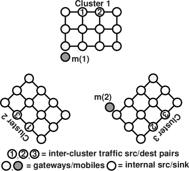
Figure 3.4: $3\times 4$ ICN used in simulations for Section 3.7.1. We also simulate with cluster size $6\times 4$. The pair of nodes labeled 1 communicate with each other, likewise for pairs 2 and 3. Under the traditional BP, the end-to-end inter-cluster delay increases (by approximately twice) as the cluster size increased from $3\times 4$ to $6\times 4$ (see Figure 3.5); however, the delay is invariant to the increase in cluster size under BP+SR. Internal nodes in the clusters maintained large queues to accommodate the inter-cluster flows under BP; under BP+SR, they did not.

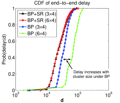
Figure 3.5: CDF of end-to-end delay for inter-cluster traffic

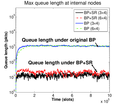
Figure 3.6: Max (type I) queue length at internal node

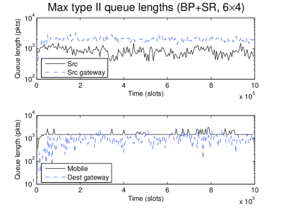
Figure 3.7: Max (type II) queue length at inter-cluster traffic nodes

3.6.4 Comparison of Two-Scale BP Algorithms

The two-scale BP algorithms we presented in Sections 3.5 and 3.6 both separate the time scale of the intermittent connectivity from the time scale of the internal connections. Under BP+SR, the rates at which sources generate data are fixed; under two-scale BP with rate control, the source rates are dynamically adjusted to maximize the sum utility. In addition, under BP+SR the internal nodes in the source cluster maintain queues for the gateways, instead of inter-cluster destinations, which allows the inter-cluster source to perform source routing. This, however, cannot be done when rate control is implemented because the inter-cluster congestion signal cannot be passed back to the inter-cluster flow source; when the inter-cluster source maintains queues for gateways and not for inter-cluster destinations, the large gateway queues can signal congestion for gateways and not for the inter-cluster destination.

3.7 Experimental Results

We present two sets of experimental results; one for two-scale BP with queue reduction (BP+SR) and another with rate control. The gain of the BP+SR compared to traditional BP is proportional to the product of the network size and the time scale of the intermittent connections. In small size networks, if the time scale of intermittent connection is large, we will also see a significant gain of the BP+SR.

Because of the limited size of our wireless testbed, we instead simulate a large network for BP+SR.

3.7.1 Two-Scale BP with Queue Reduction: BP+SR

We consider two networks. The first network consists of three clusters, with each cluster composed of 12 nodes ($3\times 4$); the second network consists of three clusters, with each cluster composed of 24 nodes ($6\times 4$). Figure 3.4 is the first network we simulate. There are three pairs of inter-cluster traffic sources/sinks, labeled with 1, 2 and 3, i.e. the two nodes labeled with 1 communicate with each other and likewise for 2’s and 3’s. The inter-cluster traffic sources generate data at a rate of 0.4 pkts/time slot. Mobile $m(1)$ comes into contact with gateways $g(i,1)$, $i=1,2,3$ only; similarly for $m(2)$. $T$ is set to 1000. In the simulation, we have randomly generated intra-cluster traffic, such that the combined intra- and inter-cluster traffic utilizes all internal links at 90% of their capacity. Each internal link has a capacity of 1 pkt/time slot. $\eta$ is set to 10. (If $\eta$ is too large, then the queue lengths would fluctuate by large amounts. If $\eta$ is too small, then the transfer algorithms Eq. (3.2), (3.3), and (3.4) would need to be executed often, increasing the processing burden.)

The probability that mobile $m(1)$ goes to gateway $g((i+1~{}\text{mod}~{}3),1)$ when it is at gateway $g(i,1)$ is 0.8 (gateway $g(i,1)$ belongs to cluster $i$); the probabilities that it stays at $g(i,1)$ or goes to $g((i-1~{}\text{mod}~{}3),1)$ both equal to 0.1. The probability that mobile $m(2)$ goes to $g((i-1~{}\text{mod}~{}3),2)$ is 0.8; the probabilities that it stay or goes to $g((i+1~{}\text{mod}~{}3),2)$ both equal to 0.1.

The number of packet transferred per contact between a mobile and a gateway is $1500$ pkts/contact ($R=1500$ pkts/contact).

We compare our BP+SR to the traditional BP, as the traditional BP (and its variants) is the only other throughput optimal routing algorithm. Figure 3.6 shows the evolution of the longest queue under BP and the evolution of the longest type-I queue under BP+SR. We can see that the longest type I queue is substantially smaller than the longest queue under BP. In our simulations, we found that under BP each node in the network had six queues of order $\Theta(T)$, corresponding to the six different inter-cluster traffic destinations. Under BP+SR, each inter-cluster source had two queues of order $\Theta(T)$, corresponding to the two gateways in each cluster. The other nodes with $\Theta(T)$ queues were gateways and mobiles.

In Figure 3.5, we show the CDF of the total end-to-end packet delays for inter-cluster traffic. The average end-to-end delay under BP+SR is roughly 28,000 time slots in both $3\times 4$ and $6\times 4$ cases; the delay under BP is 38,000 time slots in $3\times 4$ case and 78,000 in $6\times 4$ case. As discussed in Section 3.5.4, the delay doubled under BP as the cluster size doubled. The delays for intra-cluster flows stayed the same under BP+SR; BP+SR and BP both showed short delays for intra-cluster flows.

3.7.2 Two-Scale BP with Rate Control: Implementation

We implemented our two-scale BP on our 16-node testbed. Our implementation consists of two parts. The first part is the modification of the MadWifi wireless device driver for Atheros 5212 to support differentiated levels of channel access on a frame-by-frame basis through varying MAC contention parameters such as AIFS and the contention window sizes. The second part is our implementation of the modified back-pressure routing algorithm on the Click Modular Router [39], which utilizes the modified MadWifi to approximately solve the MaxWeight optimization problem (3.5) without global knowledge. We describe each part below.

MAC and PHY: We modified the MadWifi driver so that it supports four hardware queues, with each queue having different AIFS, $\text{CW}_{\max}$ and $\text{CW}_{\min}$ values shown in Table 3.1. (When two wireless transmissions contend for access to the same channel, the wireless transmission with smaller MAC parameter values will statistically have more access.) Each hardware queue is given a priority number ranging from 0 to 3. The modified device driver inspects the TOS field of the IP header of a packet, and injects it into the hardware queue with the same priority number as the TOS field. If the BP (Click-layer) queue difference between the source hop and the destination hop is greater than or equal to 25, between 24 and 14, between 13 and 6, and lower than or equal to 5, we assign TOS levels 0, 1, 2 and 3, respectively (we represent this mapping by the threshold array $L=\{25,13,5\}$). Here, the threshold arrays are chosen experimentally. If the thresholds were too close to or too far from the optimal, we did not observe desired behaviors, i.e., a pair of nodes with a large queue difference should have more access to the channel than another pair with a smaller difference. In our implementation, only one transmission packet/frame is stored in the hardware queues at a node at any given time. Our modification of the MadWifi device driver is very similar to the one in [78], with only minor differences.

Routing and Rate Control: We have implemented the traditional as well as the modified back-pressure algorithm (presented in Section 3.6.3) in the Click Modular Router. Each packet (with 1KB payload) that is sent out is assigned a value between 0 to 3 that is written to the TOS field. The assigned value depends on the queue length difference that the wireless transmission source has with the next-hop destination. Each node broadcasts a beacon on its wireless card every 500msecs. The beacon contains the information about the queues the node maintains. The nodes also use the beacons to discover their neighbors. All data packets received by a node are acknowledged, and the BP ACKs sent to the transmitting node also contain the queue information. Thus, ACKs and beacons are used to calculate the queue differences. (IEEE 802.11 ACKs are transmitted, but they are not used by the back-pressure implementation layer.) The transmitting node retransmits a data packet if an ACK for that packet is not received within 250msecs. The hop-by-hop ACK guarantees that all packets are received correctly by the final destination, and the ACKs are also used to throttle the transmission rate. We did not use any RTS-CTS in our implementation.

A source node inspects the queue for its destination every 5msecs. It runs the back-pressure rate control algorithm in Eq. (3.24) with $\kappa=3;$ i.e., it generates three packets if (3.24) is positive, and generates no packet other-wise (let this variable be NumGen). Then it uses the following update algorithm to estimate the rate $x$ (in Bps):

$$x=0.999x+0.001\frac{\text{packet\_size $\times$ NumGen}}{5\text{msecs}}.$$

Priority #	0	1	2	3
AIFS	1	3	5	7
CWmin	1	7	31	255
CWmax	7	63	255	1023

Table 3.1: MAC scheduling parameters of the four MadWifi hardware queues

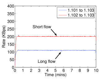
(a) $K_{1}=K_{2}=200$. The short flow rate should be two times the long flow rate.

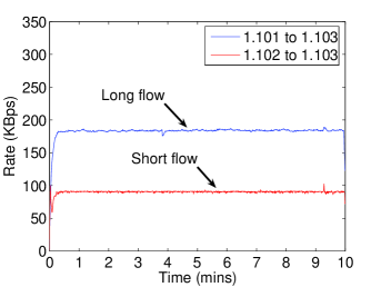
(b) $K_{1}=800,~{}K_{2}=200$. The long flow rate should be two times the short flow rate.

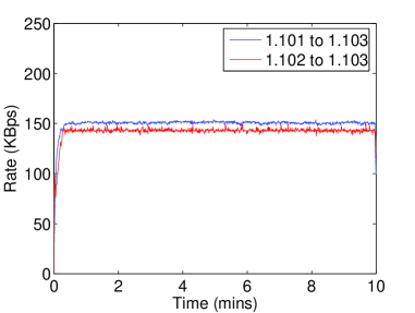
(c) $K_{1}=400,~{}K_{2}=200$. The long and short flows should get the same rate.

Figure 3.8: Rate allocations in 1.101-1.102-1.103 line network. We can control which flow gets more rate by controlling the utility function parameters $K_{1}$ and $K_{2}$. As $K_{1}$ increases relative to $K_{2}$, the long flow gets more and more rate.

On our MadWifi+Click platform, we implemented the two-scale BP with rate control algorithm for intermittently connected networks. We emphasize that the focus of our work is not an implementation of traditional back-pressure routing with the modified driver; rather, our aim is to decouple the two time scales (mobile-gateway and internal-internal) in such networks. In order to do this, we first conducted an experiment with the traditional BP on a single time-scale line network. The single time-scale line network consists of three nodes 1.101, 1.102, and 1.103 arranged in a line. We have two flows: the long flow originates from 1.101 and is destined for 1.103. The short flow originates from 1.102 and is destined for 1.103. The utility functions for long and short flow are $K_{1}\log(x_{1})$ and $K_{2}\log(x_{2})$, respectively. The rate allocations for various values of $K_{1}$ and $K_{2}$ are shown in Figures 3.8(b), 3.8(a), 3.8(c). We set $L=\{25,13,5\}$.

The optimal rate allocation is given by the solution to the following optimization problem. Let $f_{1}$ and $f_{2}$ be the fractions of time that the links 1.101-1.102 and 1.102-1.103 are active, respectively. Due to the coupled wireless interference constraint, $f_{1}+f_{2}\leq 1$. The optimal rate allocation can then be obtained by solving

maximize $$K_{1}\log(x_{1})+K_{2}\log(x_{2})$$ (3.25)

subject to $$f_{1}+f_{2}\leq 1$$

$$x_{1}\leq f_{1}C$$

$$x_{1}+x_{2}\leq f_{2}C$$

assuming that both links 1.101-1.102 and 1.102-1.103 have the same link capacity $C$. ($C$ is the one hop transmission rate between two nodes with no other transmissions in the range and was measured to be around 465KBps.) When $K_{1}=K_{2}=200$, the short and long flow rates we experimentally obtained were 200KBps and 110KBps, respectively. When $K_{1}=800$, $K_{2}=200$, the short and long rates obtained were 90KBps and 180KBps, respectively. When $K_{1}=400$, $K_{2}=200$, the short and long rates were 145KBps and 150KBps, respectively. The experimentally obtained rate allocations are approximately identical to the rate allocation obtained by solving the optimization problem (3.25)

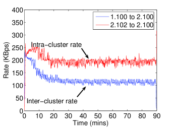
(a) $K_{1}=K_{2}=200$. Intra-rate should be $2\times$ inter-rate.

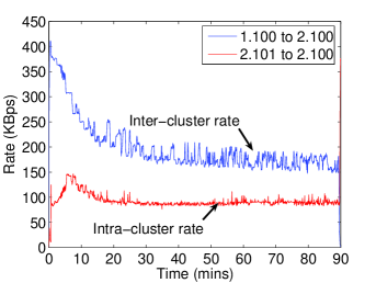
(b) $K_{1}=800,~{}K_{2}=200$. Inter-rate should be $2\times$ intra-rate.

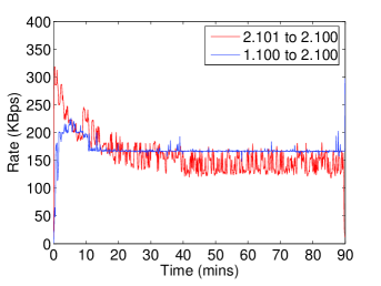
(c) $K_{1}=400,~{}K_{2}=200$. Intra- and inter-rates should be equal.

Figure 3.9: Rate allocation in the network shown in Figure 3.1 (compare against optimal rate allocations in Figures 3.8(a), 3.8(b), and 3.8(c)). The presence of the intermittent link is hidden both to the inter- and intra-cluster sources since they achieve the same rates in the network shown in Figure 3.1 as in the two-hop 1.101-1.102-1.103 line network.

3.7.3 Verification on a Line Network

Utility Maximizing Performance

We experimentally verify our algorithm on a simple intermittently connected line network shown in Figure 3.1 with $N_{c}=2$. We used a 100Mbps Cisco switch to emulate the mobile-gateway contacts. Each gateway node is equipped with one wireless card and an Ethernet port. The gateways use the wireless card to communicate with the internal nodes and the Ethernet port to communicate with the “mobile.”

On each contact, up to 6000 packets can be transferred. Each packet has a payload of 1KB, in addition to IP and Ethernet and the modified BP headers (roughly 6MB per contact). The mobile contact node switched clusters every 10 seconds, so two consecutive contacts at a gateway are 20 seconds apart. Thus, the average rate (averaged over many contacts) from the source cluster (the left cluster) to the destination cluster (the right cluster) is 300KBps. We also chose $T=6000$ and $L=\{25,13,5\}$.

The purpose of the modified BP algorithm is to have the inter-cluster traffic source be totally unaware of the mobile-gateway contacts, and to disturb any intra-cluster traffic as little as possible. We also want to obtain utility maximizing rate allocation, even though the clusters are physically separated.

Let $x_{1}$ denote the inter-cluster rate, and $x_{2}$ denote the intra-cluster rate. The utility functions for inter- and intra-cluster traffics are $U_{1}(x_{1})=K_{1}\log(x_{1})$ and $U_{2}(x_{2})=K_{2}\log(x_{2})$, respectively. We made sure the only bottleneck is the destination cluster. (If the bottlenecks are either the source cluster or the mobile-gateway contacts, this could easily be learned by the source.) Thus, the optimal rate allocation is the solution to the maximization problem (3.25) (with $f_{1}$ and $f_{2}$ denoting the fraction of time the wireless channel 2.103-2.101 and 2.101-2.100 are active, respectively). In summary:

• Recall that the traditional BP rate controller fails to give an optimal rate allocation (unless a large scaling is done, resulting in large queue sizes), and resulted in low inter-cluster rates as seen in Figure 3.2(a). However, using the modified BP, we get a high, sustained throughput for both the inter- and intra-cluster flows, and their rates are (shown Figures 3.9(a), 3.9(c) and 3.9(b)) close to the theoretically computed values. The rates are also close to the ones obtained in “Routing and Rate Control” portion of section 3.7.2 (shown in Figures 3.8(a), 3.8(b) and 3.8(c)). Thus, the modified BP successfully hides the presence of the intermittent links.

• We also verify that large queues occur only at gateways; the queue sizes at gateways were $\approx 5\times 10^{4}$. The queues at internal nodes were small, roughly $\approx 10$.

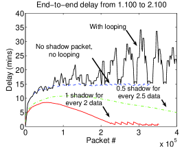
Figure 3.10: We can decrease the end-to-end inter-cluster delay first by preventing packet looping (dashed) and second by using shadow packets. As we use more and more shadow packets per data packet, the delay decreases faster.

End-to-End Delay: Shadow Packets

We compare the end-to-end delay that inter- and intra-cluster packets experience. Since inter-cluster packets must pass through the gateways and mobiles with large queues, they incur large delays. One factor causing the large inter-cluster packet delay is that some packets are “looping” between the gateways and the mobile. (“Looping” through large FIFO queues a few times can increase delays significantly.) When we prevent this looping, we get inter-cluster delay shown in Figure 3.10. (This looping is prevented only at gateways and mobiles. Looping is prevented by never having the mobile transmit each packet back to the gateway from which it was received the packet.)

Another factor that contributes to the large inter-cluster delays is that our utility-maximizing rate controller operates very close to the boundary of the capacity region. This is known to require large queues and can thus cause long delays. The authors in [14], [31] deal with this problem by introducing the notion of shadow packets and queues. Their essential idea here is to trade-off throughput for low delays. Our implementation of shadow packets is as follows:

Shadow packet implementation: For every $\kappa=3$ packets that the inter-cluster source injects into its queue according to Eq. (3.24), it marks one red (or shadow). The other two packets are marked blue (data). These shadow packets are dummy packets and do not contain any useful data (but still have 1KB payload). The blue packets contain real data. Thus, the real, useful rate is $0.66x$. The gateways and mobiles have two FIFO sub-queues for each inter-cluster destination. The red and blue packets are separated into these two sub-queues. The blue packets get transmission priority over the red packets, i.e. shadow packets are transmitted if and only if there are no blue packets that can be served. The total size (blue queue size + red queue size) is used for back-pressure routing.

The end-to-end delay with shadow packets is shown in Figure 3.10. The delay is measured only for the data packets. (We also did another experiment where we send 1 shadow packet for every 5 data packets on average (the green dash-dot curve in Figure 3.10). The two shadow packet experiments were done for 60 minutes. When the rate of shadow packet generation is 0.2/per data packet, the experiment was not long enough for the delay to converge to the minimum, but from the figure, it is clear that the algorithm with shadow packets significantly has a significantly smaller delay than that without shadow packets.) The delay curve first increases as we first need to build large queues at the gateways and mobiles. But as the real packets have priority, only the dummy, shadow packets are left behind to hold the steady-state queue sizes required for back-pressure to work. The inter-cluster delay decreased from roughly 15mins to roughly 1-2mins using shadow packets.

3.8 Experimental Results from Testbed

We implemented the modified back-pressure algorithm on our 16-node testbed. The network we conducted our experiment on is shown in Figure 3.13. The nodes in each cluster were placed only a few feet apart. (The clusters were on different channels.) Each node in a cluster uses packet filtering based on the source IP address; so for example, 1.101 can accept packets only from 1.102 and is only aware of 1.102’s presence. Thus, 1.101 will only transmit to 1.102. We are aware that any transmission from, say, 1.101 causes interference on all other transmissions because the wireless range is large enough to cover the entire cluster. However, a node can receive only one transmission at a time, and a failed transmission from, say, 1.103 (which will also transmit to 1.102 only) to 1.102 due to the interference caused by a simultaneous transmission from 1.101 would not have been received by 1.102 anyways even if the nodes were placed farther apart. (We are aware that the way we have closely laid out the nodes to conduct our experiment does not completely model the network depicted in Figure 3.13. For example, as depicted in the figure the nodes 1.103 and 1.101 are supposedly placed far apart, but they are within each other’s transmission range. Thus, there can be a collision between transmissions from 1.101 and 1.103 in the depicted network, but not in our physical network (because of CSMA). However, in practice the carrier sensing range of 802.11 is larger than the transmission range. Hence, the network we are actually modeling is where the nodes 1.101 and 1.103 are out of each other’s transmission range, but still within the carrier sense range.) Thus, placing the nodes close does not make our experimental results less valid.

Using a 100Mbps switch to emulate the mobile-gateway contacts, up to 6000 packets can be transmitted between a mobile and a gateway (so up to 12000 packets total) per contact. We picked $T=6000$, $\kappa=\eta=3$, and used queue difference levels $L=\{25,13,5\}$. After the contact is finished, the mobiles pick one of the other two gateways randomly, and initiate another contact 14 seconds later. We are aware that 14 seconds is not long enough to model most mobility in the real world. However, we picked 14 seconds to speed up our experiments so that we can have many contacts within a reasonable amount of time. Finally, all flows have the same utility function of $200\log(\cdot)$ in this study.

In summary, we have the following results from our experiment on the network in Figure 3.13:

• We observed that even in this larger network, the intra-cluster queues remain very small (between 10-15 pkts). Only the inter-cluster flows suffer large delays due to longer queues (between $10^{4}$ and $3\times 10^{4}$ pkts).

• Furthermore, using our implementation of the shadow queues and packets (the idea was proposed by the authors in [14]; we have developed an implementation for intermittently connected networks), we can “back-off” from operating on the boundary of the throughput region (i.e., utility optimal), and improve the delay performance for the inter-cluster flows; the inter-cluster delay decreased from $\approx$ 20 mins (blue, solid trace in Figure 3.12) to $\approx$ 2 mins using our shadow packets (red, dashed traces in Figure 3.12).

• To get a baseline on the approximate values we should expect, we used the fluid deterministic optimization (that ignores ACKs, collisions, retransmissions) to obtain the “optimal” rate allocations to be $x_{1}=106$, $x_{2}=83$, $x_{3}=191$, $x_{4}=146$ and $x_{5}=87$ (all KBps). Our experimental numbers are $x_{1}=84$, $x_{2}=68$, $x_{3}=120$, $x_{4}=107$ and $x_{5}=86$ (all KBps). The rates differ from the fluid approximation anywhere from a few percent to about 40%. One source of the discrepancy is that the theoretical framework as in Eq. (3.25) assumes a fluid model with no contention loss and exponential back-offs, and does not model the hop-by-hop ACKs we used. In practice, there are many packet collisions that trigger the exponential back-offs that decrease the “link capacity” in the (idealized) fluid model.

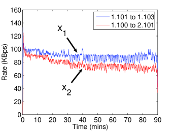
(a) Rates $x_{1}$ and $x_{2}$ in the 5.22GHz cluster

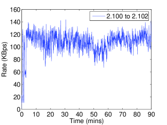
(b) Rate $x_{3}$ in the 5.26GHz cluster

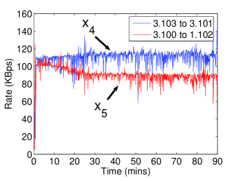
(c) Rates for $x_{4}$ and $x_{5}$ in the 5.30GHz cluster

Figure 3.11: Rate allocation in the 16-node network. See Figure 3.13 for the labels $x_{1}$, $x_{2}$, $x_{3}$, $x_{4}$ and $x_{5}$. $x_{2}$ and $x_{5}$ are inter-cluster flows.

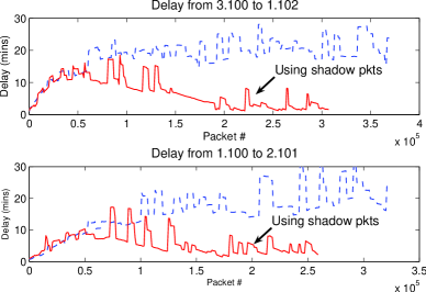
Figure 3.12: Inter-cluster delays in the network in Figure 3.13 (red, solid=using 1 shadow packet for every 2 data packets)

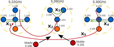
Figure 3.13: Our experimental network with 16 nodes

3.9 Appendix

3.9.1 More Comments on Overlay Network

It has been shown in [50] that by using the packet transfer algorithms (3.2), (3.3) and (3.4), the rate $\kappa_{a}^{b}[\tau]$ (pkts/time slot) at which node $a$ transfers packets out of $u_{a}^{b^{*}}$ to $q_{a}^{b}$ converges in each super time slot $\tau$. (For eqns. (3.2) and (3.4), $b^{*}$ is $b$; for eqn. (3.3), $b^{*}$ is $l_{a,b}[\tau]$.) We assume that each super time slot $\tau$ is long enough for this convergence to take place. (Hence, the rate at which $a$ transmits to $b$ converges to $\kappa_{a}^{b}[\tau]$.) In addition, within each cluster $\mathcal{C}$

$$\sum_{g_{s}\in\mathcal{H}_{\mathcal{C}}}\theta_{s}^{g_{s}}[\tau]\kappa_{s}^{g_{s}}[\tau]+\sum_{g_{1},g_{2}\in\mathcal{H}_{\mathcal{C}}}\theta_{g_{1}}^{g_{2}}[\tau]\kappa_{g_{1}}^{g_{2}}[\tau]+\sum_{g_{d}\in\mathcal{H}_{\mathcal{C}}}\theta_{g_{d}}^{d}[\tau]\kappa_{g_{d}}^{d}[\tau]$$

is maximized subject to the constraint

$$\textbf{x}_{\text{intra}(\mathcal{C})}\bigcup\left\{\kappa_{a}^{b}[\tau]~{}:~{}a,b\in\mathcal{C}\right\}$$

is supportable in $\mathcal{C}$.

We will use $\kappa_{m}^{g}[\tau]$ (either 0 or $R/T$) to denote the rate (pkts/time slot) at which mobile $m$ transmits to gateway $t$ in super time slot $\tau$; likewise for $\kappa_{g}^{m}[\tau]$.

Let $\kappa_{(a,b)}^{c}[\tau]$ denote the rate at which packets from $u_{a}^{c}$ are transmitted from $a$ to $b$ in super time slot $\tau$. For example, $\kappa_{(g_{1},g_{2})}^{g_{d}}[\tau]$ is the rate the gateway $g_{1}$ transfers to $g_{2}$ the packets destined for $g_{d}$ out of queue $u_{g_{1}}^{g_{d}}$.

3.9.2 Notations and definitions needed for the proof of Theorem 2

$\Delta u_{n}^{j}[\tau]=u_{n}^{j}[\tau+1]-u_{n}^{j}[\tau]$

We group the inputs and outputs and the exogenous arrivals as follows to simplify our analysis of type II queues. For each $u_{n}^{l}$ at node $n$, we have:

$$x_{in(n)}^{l}=\left\{\begin{array}[]{ll}\sum_{[n,d]\in\mathcal{F}}\sum_{g_{d}\in\mathcal{H}_{\mathcal{C}(d)}}x_{n,l}^{g_{d},d}&\text{if }n\in\mathcal{I}_{\mathcal{C}(n)},l\in\mathcal{H}_{\mathcal{C}(n)}\\ \sum_{[s,l]\in\mathcal{F}}\sum_{g_{s}\in\mathcal{H}_{\mathcal{C}(s)}}x_{s,g_{s}}^{n,l}&\text{if }n\in\mathcal{H}_{\mathcal{C}(l)},l\in\mathcal{I}_{\mathcal{C}(l)}\\ \sum_{[s,d]\in\mathcal{F}}x_{s,n}^{l,d}&\text{if }n\in\mathcal{H}_{\mathcal{C}(n)},l\in\mathcal{H}_{\mathcal{C}(l)},\text{and }\mathcal{C}(n)\neq\mathcal{C}(l)\\ \end{array}\right.$$

$$\kappa_{in(n)}^{l}=\left\{\begin{array}[]{ll}\sum_{i\in\mathcal{H}_{\mathcal{C}(n)}\bigcup\mathcal{M}}\kappa_{(i,n)}^{j}&\text{if }n\in\mathcal{H}_{\mathcal{C}(n)}\bigcup\mathcal{M}\\ 0&\text{else}\end{array}\right.$$

$$\kappa_{out(n)}^{l}=\left\{\begin{array}[]{ll}\kappa_{n}^{l}&\text{if }n\in\mathcal{I}_{\mathcal{C}(n)},l\in\mathcal{H}_{\mathcal{C}(n)}\\ \kappa_{n}^{l}&\text{if }n\in\mathcal{H}_{\mathcal{C}(l)},l\in\mathcal{I}_{\mathcal{C}(l)}\\ \sum_{i\in\mathcal{H}_{\mathcal{C}(n)}\bigcup\mathcal{M}}\kappa_{(n,i)}^{l}&\text{if }n\in\mathcal{H}_{\mathcal{C}(n)}\bigcup\mathcal{M}\end{array}\right.$$

The conservation rule for type II queues is thus $x_{in(n)}^{j}+\kappa_{in(n)}^{j}=\kappa_{out(n)}^{j}$. For regulated type II queues, the queue dynamics are

$$u_{n}^{j}[\tau+1]-u_{n}^{j}[\tau]=T\left(y_{n}^{j}[\tau]+\kappa_{in(n)}^{j}[\tau]-\kappa_{out(n)}^{j}[\tau]+z_{n}^{j}[\tau]\right);$$

for unregulated type II queues,

$$u_{n}^{j}[\tau+1]-u_{n}^{j}[\tau]=T\left(x_{n}^{j}[\tau]+\kappa_{in(n)}^{j}[\tau]-\kappa_{out(n)}^{j}[\tau]+z_{n}^{j}[\tau]\right).$$

$z_{n}^{j}[\tau]$ is the unused rate (pkts/time slot) in super time slot $\tau$ when there are not enough packets in the type II queue;

$$z_{n}^{j}[\tau]=\max\{\kappa_{out(n)}^{j}[\tau]-x_{n}^{j}[\tau]-\kappa_{in(n)}^{j}[\tau]-u_{n}^{j}[\tau],0\}$$

if $u_{n}^{j}$ is unregulated.

$$z_{n}^{j}[\tau]=\max\{\kappa_{out(n)}^{j}[\tau]-y_{n}^{j}[\tau]-\kappa_{in(n)}^{j}[\tau]-u_{n}^{j}[\tau],0\}$$

if $u_{n}^{j}$ is regulated.

Regulated or not, we have

$$u_{n}^{j}[\tau+1]-u_{n}^{j}[\tau] \leq T\left((1+\delta)x_{n}^{j}[\tau]+\kappa_{in(n)}^{j}[\tau]-\kappa_{out(n)}^{j}[\tau]+z_{n}^{j}[\tau]\right).~{}~{}~{}~{}~{}~{}~{}$$ (3.29)

$\Gamma$

We define

$$\mu_{(m(j),g(i,j))} = \frac{\pi_{m(j)}(i)R}{T},$$

$$\mu_{(g(i,j),m(j))} = \frac{\pi_{m(j)}(i)R}{T},$$

and

$$\vec{\mu}_{\mathcal{M}}=\left\{\mu_{(m(j),g(i,j))},\mu_{(g(i,j),m(j))}\right\}_{i,j}.$$

Note that $\vec{\mu}_{\mathcal{M}}$ is in the unit of packets/time slot. We assume that the transmissions between mobiles and gateways do not cause interference to other transmissions.

Define the network graph $\mathcal{G}=(\mathcal{N},\mathcal{L})$ where $\mathcal{N}=\left(\bigcup_{\mathcal{C}_{i}}\mathcal{N}_{C_{i}}\right)\bigcup\mathcal{M}$ and

$$\mathcal{L}=\left(\bigcup_{\mathcal{C}_{i}}\mathcal{L}_{\mathcal{C}_{i}}\right)\bigcup\left\{(m(j),g(i,j)),(g(i,j),m(j))~{}:~{}i,j\right\}.$$

Let

$$\Gamma=\left(\bigcup_{\mathcal{C}_{i}}\Gamma_{\mathcal{C}_{i}}\right)\bigcup\vec{\mu}_{\mathcal{M}}.$$

Let $\mu_{(n_{1},n_{2})}^{[s,d]}$ be the rate at which the flow $[s,d]$ is served over the link $(n_{1},n_{2})\in\mathcal{L}$. We say x is supportable if there exists $\vec{\mu}\in\Gamma$ such that:

1. For any node $n_{1}\in\mathcal{N}$ and for all flows $[s,d]$,

   $$x_{s}^{d}1_{\{s=n_{1}\}}+\sum_{(n_{2},n_{1})\in\mathcal{L}}\mu_{(n_{2},n_{1})}^{[s,d]}=\sum_{(n_{1},n_{3})\in\mathcal{L}}\mu_{(n_{1},n_{3})}^{[s,d]}.$$

2. $\left\{\sum_{[s,d]}\mu_{(n_{1},n_{2})}^{[s,d]}\right\}\in\Gamma$.

We say $\textbf{x}_{\text{intra}(\mathcal{C}_{i})}$ is supportable in $\mathcal{C}_{i}$ if the conditions 1) and 2) above hold with $\mathcal{L}$ and $\Gamma$ replaced with $\mathcal{L}_{\mathcal{C}_{i}}$ and $\Gamma_{\mathcal{C}_{i}}$, respectively.

$\kappa_{\min}$, $\kappa_{\max}$, and $N_{u}$

Let

$$\kappa_{\min}=\min\left\{\min_{\mathcal{C}}\left\{\max_{(a,b)\in\mathcal{C}~{}:~{}\textbf{x}_{\text{inter}(\mathcal{C})}\bigcup\kappa_{a}^{b}\in\Gamma_{\mathcal{C}}}\kappa_{a}^{b}\right\},R/T\right\}$$

and

$$\kappa_{\max}=\max\left\{\max_{\mathcal{C}}\left\{\max_{(a,b)\in\mathcal{C}~{}:~{}\textbf{x}_{\text{inter}(\mathcal{C})}\bigcup\kappa_{a}^{b}\in\Gamma_{\mathcal{C}}}\kappa_{a}^{b}\right\},R/T\right\}.$$

We assume that $\eta>\kappa_{\max}$. We will see in lemma 4 that there is at least one type II queue in each cluster that is guaranteed to transmit or receive at rate $\kappa_{\min}$ or higher. $\kappa_{\max}$ is the maximum rate at which any type II queue in the network could change. Lastly, let

$$N_{u} = N_{s}\left(N_{g}+\max_{\mathcal{C}}\{\max\{\text{\# of inter-cluster traffic srcs}\right.$$

$$\left.\text{in $\mathcal{C}$},\text{\# of inter-cluster traffic dest. in $\mathcal{C}$}\}\}\right)+N_{g}$$

and let $\vec{\kappa}=\{\kappa_{a}^{b}\}$. Note that $N_{u}>$ # of type II queues maintained at any node, and $N_{u}>$ # of nodes with at least one type II queue.

3.9.3 Proof of Theorem 2

We will first bound the queue lengths when the routing algorithms (Eq. (3.1), (3.2), (3.3), and (3.4)) are updated every $\tilde{T}$ super time slots; we will refer $\tilde{T}$ super time slots as a super-super time slot. We assume that $\tilde{T}$ is large enough so that for any mobile $m$ and any gateway $g$ $m$ comes into contact with, $m$ makes at least $(1+\epsilon)^{-1}(\pi_{m})_{g}\tilde{T}$ contacts with $g$ over $\tilde{T}$ super time slots. Let $\tilde{\tau}$ denote $\tilde{\tau}$-th super-super time slot. We will use this bound to obtain the upper bound when routing algorithms are updated every super time slot.

We prove stability using Lyapunov analysis. The Lyapunov function we choose is a quadratic function of the type II queue length. We will show that if any one of the type II queues reaches a certain threshold, the Lyapunov function will start to decrease. This will show that the Lyapunov function is bounded, and that the queues are bounded as well.

We will use $\kappa_{a}^{b}[\tau]$ to denote the transmission rate from node $a$ to $b$ in the overlay network in super time slot $\tau$, and $\kappa_{(a,b)}^{c}[\tau]$ denote the rate at which packets from $u_{a}^{c}$ are transmitted from $a$ to $b$ in super time slot $\tau$.

We define a Lyapunov function $V[\tilde{\tau}\tilde{T}]=\sum_{n}\sum_{j}(u_{n}^{j}[\tilde{\tau}\tilde{T}])^{2}$. Let

$$\Delta_{\tilde{T}}V[\tilde{\tau}\tilde{T}] = V[(\tilde{\tau}+1)\tilde{T}]-V[\tilde{\tau}\tilde{T}]$$

$$= \sum_{n}\sum_{j}(u_{n}^{j}[(\tilde{\tau}+1)\tilde{T}])^{2}-(u_{n}^{j}[\tilde{\tau}\tilde{T}])^{2}$$

$$= \sum_{n}\sum_{j}(u_{n}^{j}[(\tilde{\tau}+1)\tilde{T}]-u_{n}^{j}[\tilde{\tau}T])$$

$$~{}~{}~{}~{}~{}\times(u_{n}^{j}[(\tilde{\tau}+1)\tilde{T}]+u_{n}^{j}[\tilde{\tau}\tilde{T}])$$

$$= \sum_{n}\sum_{j}\Delta u_{n}^{j}[\tilde{\tau}\tilde{T}](u_{n}^{j}[(\tilde{\tau}+1)\tilde{T}]+u_{n}^{j}[\tilde{\tau}\tilde{T}])$$

where

$$\Delta u_{n}^{j}[\tilde{\tau}\tilde{T}] = u_{n}^{j}[(\tilde{\tau}+1)\tilde{T}]-u_{n}^{j}[\tilde{\tau}\tilde{T}]$$ (3.30)

$$= \sum_{l=\tilde{\tau}\tilde{T}}^{(\tilde{\tau}+1)\tilde{T}-1}u_{n}^{j}[l+1]-u_{n}^{j}[l]$$

$$\leq T\sum_{l=\tilde{\tau}\tilde{T}}^{(\tilde{\tau}+1)\tilde{T}-1}\left((1+\delta)x_{n}^{j}[l]+\kappa_{in(n)}^{j}[l]-\kappa_{out(n)}^{j}[l]+z_{n}^{j}[l]\right)$$

Eq. (3.30) follows from the following queue dynamics:

$$u_{n}^{j}[\tau+1]-u_{n}^{j}[\tau] \leq T\left((1+\delta)x_{n}^{j}[\tau]+\kappa_{in(n)}^{j}[\tau]-\kappa_{out(n)}^{j}[\tau]+z_{n}^{j}[\tau]\right)~{}~{}~{}~{}~{}~{}$$ (3.31)

which we derived in Eq. (3.29). Thus,

$$\Delta_{\tilde{T}}V[\tilde{\tau}\tilde{T}] \leq T\sum_{n}\sum_{j}\sum_{l=\tilde{\tau}\tilde{T}}^{(\tilde{\tau}+1)\tilde{T}-1}\left[(1+\delta)x_{n}^{j}[l]+\kappa_{in(n)}^{j}[l]\right.$$

$$\left.-\kappa_{out(n)}^{j}[l]+z_{n}^{j}[l]\right](u_{n}^{j}[(\tilde{\tau}+1)\tilde{T}]+u_{n}^{j}[\tilde{\tau}\tilde{T}])$$

$$\leq T\sum_{n}\sum_{j}\sum_{l}\left[(1+\delta)x_{n}^{j}[l]+\kappa_{in(n)}^{j}[l]\right.$$

$$\left.-\kappa_{out(n)}^{j}[l]+z_{n}^{j}[l]\right](2u_{n}^{j}[\tilde{\tau}\tilde{T}]+\tilde{T}T\kappa_{\max})$$

$$\leq T\sum_{n}\sum_{j}\sum_{l}2u_{n}^{j}[\tilde{\tau}\tilde{T}]\left[(1+\delta)x_{n}^{j}[l]\right.$$

$$\left.+\kappa_{in(n)}^{j}[l]-\kappa_{out(n)}^{j}[l]\right]+C$$

where $C=4N_{u}^{2}(\tilde{T}T\kappa_{\max})^{2}$ because if $u_{n}^{j}[\tilde{\tau}\tilde{T}]>\tilde{T}T\kappa_{\max}$, then $z_{n}^{j}[l]=0$ since there are enough packets; and $z_{n}^{j}[l]<\kappa_{\max}$ always. ($\kappa_{\max}$ is defined in subsection 3.9.2. $\kappa_{\max}$ is the maximum rate (pkts/time slot) at which any type II queue can change.)

Let

$$A_{\textbf{x}}[\tilde{\tau}\tilde{T}] = T\sum_{n}\sum_{j}\sum_{l=\tilde{\tau}\tilde{T}}^{(\tilde{\tau}+1)\tilde{T}-1}u_{n}^{j}[\tilde{\tau}\tilde{T}]x_{in(n)}^{j}[l]$$ (3.32)

$$= T\tilde{T}\sum_{n}\sum_{j}u_{n}^{j}[\tilde{\tau}\tilde{T}]x_{in(n)}^{j}[\tilde{\tau}\tilde{T}]$$

since (3.1) is assumed to be updated every $\tilde{T}$ super time slots; let

$$B_{\kappa}[\tilde{\tau}\tilde{T}] =T\sum_{n}\sum_{j}\sum_{l=\tilde{\tau}\tilde{T}}^{(\tilde{\tau}+1)\tilde{T}-1}u_{n}^{j}[\tilde{\tau}\tilde{T}](\kappa_{out(n)}^{j}[l]-\kappa_{in(n)}^{j}[l])$$ (3.33)

$$=T\sum_{j}\sum_{(n,m)}\sum_{l=\tilde{\tau}\tilde{T}}^{(\tilde{\tau}+1)\tilde{T}-1}(u_{n}^{j}[\tilde{\tau}\tilde{T}]-u_{m}^{j}[\tilde{\tau}\tilde{T}])\kappa_{(n,m)}^{j}[l].$$

Note that since (3.1) is updated every $\tilde{T}$ super time slots,

$$A_{\textbf{x}}[\tilde{\tau}\tilde{T}]=T\tilde{T}\sum_{[s,d]\in\mathcal{F}}\min_{g_{s}\in\mathcal{H}_{\mathcal{C}(s)},g_{d}\in\mathcal{H}_{\mathcal{C}(d)}}\left(u_{s}^{g_{s}}[\tilde{\tau}\widetilde{T}]+u_{g_{s}}^{g_{d}}[\tilde{\tau}\widetilde{T}]+u_{g_{d}}^{d}[\tilde{\tau}\widetilde{T}]\right)x_{s}^{d}.$$

Then,

$$\Delta_{\tilde{T}}V[\tilde{\tau}\tilde{T}]\leq 2(1+\delta)A_{\textbf{x}}[\tilde{\tau}\tilde{T}]-2B_{\kappa}[\tilde{\tau}\tilde{T}]+C.$$ (3.34)

Since $(1+\delta+\epsilon)\textbf{x}$ is supportable, there exists $\vec{\mu}\in\Gamma$ and $\vec{\kappa}$ such that $\vec{\mu}\in\Gamma$ and

$$0=\sum_{n}\sum_{j}u_{n}^{j}[\tilde{\tau}\tilde{T}]\left((1+\delta+\epsilon)x_{in(n)}^{j}+\kappa_{in(n)}^{j}-\kappa_{out(n)}^{j}\right).$$

($\Gamma$ is defined in subsection 3.9.2. It is the convex hull of all possible schedules, including all possible mobile-gateway schedules. $\vec{\kappa}$ is a vector of possible transmission rates in the overlay network.)

Letting $\tilde{A}_{\textbf{x}}[\tilde{\tau}\tilde{T}]=T\tilde{T}\sum_{n}\sum_{j}u_{n}^{j}[\tilde{\tau}\tilde{T}]x_{in(n)}^{j}$ and

$$\tilde{B}_{\kappa}[\tilde{\tau}\tilde{T}] = T\tilde{T}\sum_{n}\sum_{j}u_{n}^{j}[\tilde{\tau}\tilde{T}](\kappa_{out(n)}^{j}-\kappa_{in(n)}^{j})$$

$$= T\tilde{T}\sum_{j}\sum_{(n,m)}(u_{n}^{j}[\tilde{\tau}\tilde{T}]-u_{m}^{j}[\tilde{\tau}\tilde{T}])\kappa_{(n,m)}^{j},$$

we have $(1+\delta+\epsilon)\tilde{A}_{\textbf{x}}[\tilde{\tau}\tilde{T}]=\tilde{B}_{\kappa}[\tilde{\tau}\tilde{T}]$ because $(1+\delta+\epsilon)\textbf{x}$ is supportable.

Hence,

$$\Delta_{\tilde{T}}V[\tilde{\tau}\tilde{T}] \leq 2(1+\delta)A_{\textbf{x}}[\tilde{\tau}\tilde{T}]-2B_{\kappa}[\tilde{\tau}\tilde{T}]+C$$

$$-2(1+\delta+\epsilon)\tilde{A}_{\textbf{x}}[\tilde{\tau}\tilde{T}]+2\tilde{B}_{\kappa}[\tilde{\tau}\tilde{T}]$$

Since $A_{\textbf{x}}[\tilde{\tau}\tilde{T}]\leq\tilde{A}_{\textbf{x}}[\tilde{\tau}\tilde{T}]$ and $\tilde{B}_{\kappa}[\tilde{\tau}\tilde{T}]\leq B_{\kappa}[\tilde{\tau}\tilde{T}]$ (see Lemmas 3 and 4 in the Appendix of this chapter),

$$\Delta_{\tilde{T}}V[\tilde{\tau}\tilde{T}]\leq-2\epsilon\tilde{A}_{\textbf{x}}[\tilde{\tau}\tilde{T}]+C.$$

If $\tilde{A}_{\textbf{x}}[\tilde{\tau}\tilde{T}]\geq C/(2\epsilon)$, then $\Delta_{\tilde{T}}V[\tilde{\tau}\tilde{T}]\leq-C$.

If $\tilde{A}_{\textbf{x}}[\tilde{\tau}\tilde{T}]<C/(2\epsilon)$, then from Eq. (3.34) and the fact that $A_{\textbf{x}}[\tilde{\tau}\tilde{T}]\leq\tilde{A}_{\textbf{x}}[\tilde{\tau}\tilde{T}]$ we have

$$\Delta_{\tilde{T}}V[\tilde{\tau}\tilde{T}]\leq\tilde{C}-2B_{\kappa}[\tilde{\tau}\tilde{T}]$$

where $\tilde{C}=C+\frac{1+\delta}{\epsilon}C$. If there exists $(m,n)$ and $j$ such that

$$u_{m}^{j}[\tilde{\tau}\tilde{T}]-u_{n}^{j}[\tilde{\tau}\tilde{T}]\geq\frac{\tilde{C}}{T\tilde{T}\kappa_{\min}}$$ (3.35)

then $\Delta V_{\tilde{T}}[\tilde{\tau}\tilde{T}]\leq-\tilde{C}$ (plug Eq. (3.35) into Eq. (3.33)). ($\kappa_{\min}$ is defined in subsection 3.9.2. It is the minimum rate at which at least one type II queue is guaranteed to change.)

Such $(m,n)$ and $j$ that satisfy Eq. (3.35) exist if there exists $m$ such that $u_{m}^{j}[\tilde{\tau}\tilde{T}]\geq\frac{N_{u}\tilde{C}}{T\tilde{T}\kappa_{\min}}$ since $u_{m}^{m}[\tilde{\tau}\tilde{T}]=0$ and there are $N_{u}$ nodes with type II queues ($N_{u}$ is defined in subsection 3.9.2).

Thus, $V[\tilde{\tau}\tilde{T}]\leq\left(\bar{K}\right)^{2}$ where

$$\bar{K}=N_{u}\left(\frac{N_{u}\tilde{C}}{T\tilde{T}\kappa_{\min}}+\kappa_{\max}T\tilde{T}\right)$$

which implies that

$$u_{n}^{j}[\tilde{\tau}\tilde{T}]\leq\bar{K}$$ (3.36)

for all $n$ and $j$ when our algorithm is updated every $\tilde{T}$ super time slots.

We now consider the real queue $\tilde{u}_{n}^{j}[\tilde{\tau}\tilde{T}]$ where $n$ and $j$ are gateways. Let $M_{n}^{j}[\tilde{\tau}\tilde{T}]$ be the number of packets in the network that are yet to arrive at the regulated queue $u_{n}^{j}$ yet. Assume there is $\tilde{\tau}_{0}$ such that for $\tilde{\tau}>\tilde{\tau}_{0}$, we have

$$M_{n}^{j}[\tilde{\tau}\tilde{T}]>N_{u}\bar{K}+T\tilde{T}\kappa_{\max}$$

which implies $\tilde{u}_{n}^{j}[\tilde{\tau}\tilde{T}]>T\tilde{T}\kappa_{\max}$ due to Eq. (3.36). The packets that did not arrive at $u_{n}^{j}$ must be held some where, and because there are fewer than $N_{u}$ nodes with type II queues and each regulated type II queue is bounded as in Eq. (3.36), we must have $\tilde{u}_{n}^{j}[\tilde{\tau}\tilde{T}]>T\tilde{T}\kappa_{\max}$. Thus, we get

$$M_{n}^{j}[(\tilde{\tau}+1)\tilde{T}] = \tilde{T}T\left(\sum_{[s,d]\in\mathcal{F}_{\text{inter}}}x_{s,n}^{j,d}[\tilde{\tau}T]\right)+M_{n}^{j}[\tilde{\tau}\tilde{T}]-\tilde{T}Ty_{n}^{j}[\tilde{\tau}T]$$

$$\leq M_{n}^{j}[\tilde{\tau}\tilde{T}]$$

which implies that for $\tilde{\tau}>\tilde{\tau}_{0}$

$$M_{n}^{j}[\tilde{\tau}\widetilde{T}]\leq\max\left\{M_{n}^{j}[\tilde{\tau}_{0}\tilde{T}],N_{u}\bar{K}+2T\tilde{T}\kappa_{\max}\right\}.$$

Thus, real queues $\tilde{u}_{n}^{j}[\tilde{\tau}\tilde{T}]$ are bounded as well.

We now examine the real queue when $n$ is a gateway and $j$ is an inter-cluster traffic destination. Let $\mathcal{B}$ denote the bound on $\tilde{u}_{n}^{j}[\tilde{t}\widetilde{T}]$ where $n$ and $j$ are gateways. Let $M_{n}^{j}[\tilde{\tau}\tilde{T}]$ be the number of packets in the network that are yet to arrive at the regulated queue $u_{n}^{j}$, $n\in\cup_{\mathcal{C}}\mathcal{H}_{\mathcal{C}}$, $j\in\mathcal{I}_{\mathcal{C}(n)}$. Assume there is $\tilde{\tau}_{0}$ such that for $\tilde{\tau}>\tilde{\tau}_{0}$, we have

$$M_{n}^{j}[\tilde{\tau}\tilde{T}]>N_{u}\bar{K}+N_{g}\mathcal{B}+T\tilde{T}\kappa_{\max}$$

which implies $\tilde{u}_{n}^{j}[\tilde{\tau}\tilde{T}]>T\tilde{T}\kappa_{\max}$ due to Eq. (3.36) and since real, gateway-to-gateway queues are bounded by $\mathcal{B}$ and there are only $N_{g}$ source gateways where these packets can be. Thus, we get

$$M_{n}^{j}[(\tilde{\tau}+1)\tilde{T}] = \tilde{T}T\left(\sum_{s,g_{s}}x_{s,g_{s}}^{n,j}[\tilde{\tau}T]\right)+M_{n}^{j}[\tilde{\tau}\tilde{T}]-\tilde{T}Ty_{n}^{j}[\tilde{\tau}T]$$

$$\leq M_{n}^{j}[\tilde{\tau}\tilde{T}]$$

which implies that for $\tilde{\tau}>\tilde{\tau}_{0}$

$$M_{n}^{j}[\tilde{\tau}\widetilde{T}]\leq\max\left\{M_{n}^{j}[\tilde{\tau}_{0}\tilde{T}],N_{u}\bar{K}+N_{g}\mathcal{B}+2T\tilde{T}\kappa_{\max}\right\}.$$

Thus, real queues $\tilde{u}_{n}^{j}[\tilde{\tau}\tilde{T}]$ are bounded as well.

Now, consider when our algorithm is updated every super time slot (as is in Eq. (3.1), (3.2), (3.3) and (3.4)). We have

$$\Delta_{\tilde{T}}V[\tilde{\tau}\tilde{T}] = \sum_{n}\sum_{j}\sum_{l=\tilde{\tau}\tilde{T}}^{(\tilde{\tau}+1)\tilde{T}-1}\left(u_{n}^{j}[l+1]\right)^{2}-\left(u_{n}^{j}[l]\right)^{2}$$

$$= \sum_{n}\sum_{j}\sum_{l}\left(u_{n}^{j}[l+1]-u_{n}^{j}[l]\right)\left(u_{n}^{j}[l+1]+u_{n}^{j}[l]\right)$$

By Eq. (3.29),

$$\Delta_{\tilde{T}}V[\tilde{\tau}\tilde{T}] \leq T\sum_{n}\sum_{j}\sum_{l=\tilde{\tau}\tilde{T}}^{(\tilde{\tau}+1)\tilde{T}-1}\left[(1+\delta)x_{n}^{j}[l]+\kappa_{in(n)}^{j}[l]\right.$$

$$\left.-\kappa_{out(n)}^{j}[l]+z_{n}^{j}[l]\right](u_{n}^{j}[l+1]+u_{n}^{j}[l])$$

$$\leq T\sum_{n}\sum_{j}\sum_{l}\left[(1+\delta)x_{n}^{j}[l]+\kappa_{in(n)}^{j}[l]\right.$$

$$\left.-\kappa_{out(n)}^{j}[l]+z_{n}^{j}[l]\right](2u_{n}^{j}[l]+T\kappa_{\max})$$

$$\leq T\sum_{n}\sum_{j}\sum_{l}2u_{n}^{j}[l]\left[(1+\delta)x_{n}^{j}[l]\right.$$

$$\left.+\kappa_{in(n)}^{j}[l]-\kappa_{out(n)}^{j}[l]\right]+C^{\prime}$$

$$\leq 2(1+\delta)\hat{A}_{\textbf{x}}[\tilde{\tau}]-\hat{B}_{\kappa}[\tilde{\tau}]+C^{\prime}$$

where $C^{\prime}=4\tilde{T}N_{u}^{2}\left(T\kappa_{\max}\right)^{2}$ and

$$\hat{A}_{\textbf{x}}[\tilde{\tau}\tilde{T}]=T\sum_{n}\sum_{j}\sum_{l=\tilde{\tau}\tilde{T}}^{(\tilde{\tau}+1)\tilde{T}}u_{n}^{j}[l]x_{n}^{j}[l]$$

and

$$\hat{B}_{\kappa}[\tilde{\tau}\tilde{T}]=T\sum_{n}\sum_{j}\sum_{l=\tilde{\tau}\tilde{T}}^{(\tilde{\tau}+1)\tilde{T}}u_{n}^{j}[l]\left(\kappa_{out(n)}^{j}[l]-\kappa_{in(n)}^{j}[l]\right).$$

By Lemmas 5 and 6, $\exists~{}C_{A},C_{B}$ such that $\hat{A}_{\textbf{x}}[\tilde{\tau}\tilde{T}]\leq A_{\textbf{x}}[\tilde{\tau}\tilde{T}]+C_{A}$ and $\hat{B}_{\kappa}[\tilde{\tau}\tilde{T}]\geq B_{\kappa}[\tilde{\tau}\tilde{T}]-C_{B}$; thus, we have

$$\Delta_{\tilde{T}}V[\tilde{\tau}\widetilde{T}]\leq 2(1+\delta)A_{\textbf{x}}[\tilde{\tau}\tilde{T}]-B_{\kappa}[\tilde{\tau}\tilde{T}]+C^{\prime\prime}$$

where $C^{\prime\prime}=C^{\prime}+C_{A}+C_{B}$. Then, following the same analysis as before, we get

$$u_{n}^{j}[\tilde{\tau}\widetilde{T}]\leq N_{u}\left(\frac{N_{u}\tilde{C}^{\prime\prime}}{T\tilde{T}\kappa_{\min}}+\kappa_{\max}T\tilde{T}\right)$$

using algorithms (3.1), (3.2), (3.3) and (3.4), where $\tilde{C}^{\prime\prime}=C^{\prime\prime}+(1+\delta)C^{\prime\prime}/\epsilon$.

Following similar reasoning in [82], we can bound the real queues.

Note that the probability that the mobile does not exhibit stationary distribution in $\widetilde{T}$ super time slots is exponentially decreasing in $\widetilde{T}$. Thus, we can obtain an expected bound on the type-II queues. Furthermore, we can use theorem 1 of [50] to bound the type-I queues since in eqs. (3.2), (3.3) and (3.4), type-II queue sizes are used as a linear utility function.  

3.9.4 $\tilde{A}_{\textbf{x}}[\tilde{\tau}\tilde{T}]\geq A_{\textbf{x}}[\tilde{\tau}\tilde{T}]$

Lemma 3.

$\tilde{A}_{\textbf{x}}[\tilde{\tau}\tilde{T}]\geq A_{\textbf{x}}[\tilde{\tau}\tilde{T}]$.

Proof:

$$\tilde{A}_{\textbf{x}}[\tilde{\tau}\tilde{T}] = T\tilde{T}\sum_{[s,d]\in\mathcal{F}}\sum_{g_{s}\in\mathcal{H}_{\mathcal{C}(s)}}\sum_{g_{d}\in\mathcal{H}_{\mathcal{C}(d)}}\left(u_{s}^{g_{s}}[\tilde{\tau}\widetilde{T}]+u_{g_{s}}^{g_{d}}[\tilde{\tau}\widetilde{T}]+u_{g_{d}}^{d}[\tilde{\tau}\widetilde{T}]\right)x_{s,g_{s}}^{g_{d},d}$$

$$\geq T\tilde{T}\sum_{[s,d]\in\mathcal{F}}\min_{g_{s}\in\mathcal{H}_{\mathcal{C}(s)},g_{d}\in\mathcal{H}_{\mathcal{C}(d)}}\left(u_{s}^{g_{s}}[\tilde{\tau}\widetilde{T}]+u_{g_{s}}^{g_{d}}[\tilde{\tau}\widetilde{T}]+u_{g_{d}}^{d}[\tilde{\tau}\widetilde{T}]\right)x_{s}^{d}$$

$$= A_{\textbf{x}}[\tilde{\tau}\tilde{T}]$$

since $\sum_{g_{s}\in\mathcal{H}_{\mathcal{C}(s)}}\sum_{g_{d}\in\mathcal{H}_{\mathcal{C}(d)}}x_{s,g_{s}}^{g_{d},d}=x_{s}^{d}$, and because of algorithm (3.1) and the fact that the source routing is updated every $\tilde{T}$ super time slots.  

3.9.5 $\tilde{B}_{\kappa}[\tilde{\tau}\tilde{T}]\leq B_{\kappa}[\tilde{\tau}\tilde{T}]$

Lemma 4.

$\tilde{B}_{\kappa}[\tilde{\tau}\tilde{T}]\leq B_{\kappa}[\tilde{\tau}\tilde{T}]$.

Proof: In each cluster $\mathcal{C}$, there are intra-cluster traffics mixed with source-to-gateway relay, gateway-to-gateway relay, and gateway-to-destination relay, all of which form parts of inter-cluster traffic.

We will use the theorems from [50] to prove our lemma.

In the super-super time block $\tilde{\tau}$, let the utility of each intra-cluster traffic $[s,d]$ in $\mathcal{C}$ be $U_{[s,d]}(x_{[s,d]})=\alpha x_{[s,d]}$, where $\alpha$ is some constant.

For each source-to-gateway relay that originates from $s\in\mathcal{C}$ ending at gateway $g_{s}\in\mathcal{C}$, let the utility function be

$$U_{[s,g_{s}]}(\kappa_{s}^{g_{s}})=\theta_{s}^{g_{s}}[\tilde{\tau}\widetilde{T}]\kappa_{s}^{g_{s}}.$$

For each gateway-to-gateway relay between $g_{1}$ and $g_{2}$, let

$$U_{[g_{1},g_{2}]}(\kappa_{g_{1}}^{g_{2}})=\theta_{g_{1}}^{g_{2}}[\tilde{\tau}\widetilde{T}]\kappa_{g_{1}}^{g_{2}}.$$

For each gateway-to-destination between $g_{d}$ and $d$, let

$$U_{[g_{d},d]}(\kappa_{g_{d}}^{d})=\theta_{g_{d}}^{d}[\tilde{\tau}\widetilde{T}]\kappa_{g_{d}}^{d}.$$

We assume that $\alpha>>\theta_{s}^{g_{s}}[\tilde{\tau}\widetilde{T}],\theta_{g_{1}}^{g_{2}}[\tilde{\tau}\widetilde{T}],\theta_{g_{d}}^{d}[\tilde{\tau}\widetilde{T}]$.

It is shown in Theorem 1 of [50] that our transfer algorithms (3.2), (3.3) and (3.4) solve the optimization problem

Maximize: $$\sum U_{[s,d]}(x)+\sum U_{[s,g_{d}]}(\kappa_{s}^{g_{s}})$$

$$+\sum U_{[g_{1},g_{2}]}(\kappa_{g_{1}}^{g_{2}})+\sum U_{[g_{d},d]}(\kappa_{g_{d}}^{d})$$

Subject to: $$\{x_{[s,d]}:\mathcal{F}_{\text{intra}(\mathcal{C})}\}\bigcup\{\kappa_{a}^{b}\}\in\Gamma_{\mathcal{C}}$$

$$\{x_{[s,d]}\}\leq\textbf{x}_{\text{intra}(\mathcal{C})}$$

Since $\alpha>>\theta_{s}^{g_{s}}[\tilde{\tau}\widetilde{T}],\theta_{g_{1}}^{g_{2}}[\tilde{\tau}\widetilde{T}],\theta_{g_{d}}^{d}[\tilde{\tau}\widetilde{T}]$, we assume that the above optimization is solved with $\{x_{[s,d]}\}=\textbf{x}_{\text{intra}(\mathcal{C})}$. Then, the above optimization becomes

Maximize: $$\sum U_{[s,g_{d}]}(\kappa_{s}^{g_{s}})+\sum U_{[g_{1},g_{2}]}(\kappa_{g_{1}}^{g_{2}})+\sum U_{[g_{d},d]}(\kappa_{g_{d}}^{d})$$

Subject to: $$\textbf{x}_{\text{intra}(\mathcal{C})}\bigcup\{\kappa_{a}^{b}\}\in\Gamma_{\mathcal{C}},$$

which is solved by transfer algorithms (3.2), (3.3) and (3.4) according to [50].

Let $\{\kappa_{a}^{b}[\tilde{\tau}\widetilde{T}]\}$ be the set of values that maximize the above optimization problem. Then,

$$T\tilde{T}\sum_{j}\sum_{(n,m):n,m\notin\mathcal{M}}\left(u_{n}^{j}[\tilde{\tau}\widetilde{T}]-u_{n}^{j}[\tilde{\tau}\widetilde{T}]\right)\kappa_{(n,m)}^{j}[\tilde{\tau}\widetilde{T}]\geq$$ (3.37)

$$T\tilde{T}\sum_{j}\sum_{(n,m):n,m\notin\mathcal{M}}\left(u_{n}^{j}[\tilde{\tau}\widetilde{T}]-u_{n}^{j}[\tilde{\tau}\widetilde{T}]\right)\kappa_{(n,m)}^{j}$$

for each cluster $\mathcal{C}$.

Let $1_{\{m_{k}=g_{i,k}\}}[l]=1$ if $m(k)$ and $g(i,k)$ are in contact in super time slot $l$. We now consider the mobile-to-gateway contacts.

$$\sum_{l=0}^{\tilde{T}-1}\sum_{m_{k}\in\mathcal{M}}\sum_{g_{i,k}}1_{\{m_{k}=g_{i,k}\}}[\tilde{\tau}\widetilde{T}+l]R$$

$$\left[\left(u_{m_{k}}^{j_{(m_{k},g_{i,k})}[\tilde{\tau}\widetilde{T}]}[\tilde{\tau}\widetilde{T}]-u_{g(i,k)}^{j_{(m_{k},g_{i,k})}[\tilde{\tau}\widetilde{T}]}[\tilde{\tau}\widetilde{T}]\right)\right.$$

$$\left.+\left(u_{g(i,k)}^{j_{(g_{i,k},m_{k})}[\tilde{\tau}\widetilde{T}]}[\tilde{\tau}\widetilde{T}]-u_{m(k)}^{j_{(g_{i,k},m_{k})}[\tilde{\tau}\widetilde{T}]}[\tilde{\tau}\widetilde{T}]\right)\right]$$

$$= T\tilde{T}\sum_{m_{k}\in\mathcal{M}}\sum_{g_{i,k}}\kappa_{(m_{k},g_{i,k})}[\tilde{\tau}\widetilde{T}]\left(u_{m_{k}}^{j_{(m_{k},g_{i,k})}[\tilde{\tau}\widetilde{T}]}[\tilde{\tau}\widetilde{T}]-u_{g_{i,k}}^{j_{(m_{k},g_{i,k})}[\tilde{\tau}\widetilde{T}]}[\tilde{\tau}\widetilde{T}]\right)$$

$$+\kappa_{(g_{i,k},m_{k})}[\tilde{\tau}\widetilde{T}]\left(u_{g_{i,k}}^{j_{(g_{i,k},m_{k})}[\tilde{\tau}\widetilde{T}]}[\tilde{\tau}\widetilde{T}]-u_{m_{k}}^{j_{(g_{i,k},m_{k})}[\tilde{\tau}\widetilde{T}]}[\tilde{\tau}\widetilde{T}]\right)$$

since every super time slot $m_{k}$ and $g_{i,k}$ are in contact, $R$ packets are uploaded and downloaded and thus

$$T\tilde{T}\kappa_{(m_{k},g_{i,k})}[\tilde{\tau}\widetilde{T}] = \sum_{l=0}^{\tilde{T}-1}1_{\{m_{k}=g_{i,k}\}}[\tilde{\tau}\widetilde{T}+l]R,$$

$$T\tilde{T}\kappa_{(g_{i,k},m_{k})}[\tilde{\tau}\widetilde{T}] = \sum_{l=0}^{\tilde{T}-1}1_{\{m_{k}=g_{i,k}\}}[\tilde{\tau}\widetilde{T}+l]R.$$

Since we assumed that any mobile $m$ makes at least $(1+\gamma)^{-1}(\pi_{m})_{g}\tilde{T}$ contacts with $g$ ($g$ is any gateway $m$ can come in contact with) over $\tilde{T}$ super time slots (see proof of theorem 2), we have

$$\sum_{l=0}^{\tilde{T}-1}1_{\{m_{k}=g_{i,k}\}}[\tilde{\tau}\widetilde{T}+l]\geq(1+\gamma)^{-1}(\pi_{m_{k}})_{g_{i,k}}\tilde{T}$$

and thus

$$\text{Eq. }(\ref{eq:b_mg}) \geq \sum_{m_{k}\in\mathcal{M}}\sum_{g_{i,k}}(1+\gamma)^{-1}(\pi_{m_{k}})_{g_{i,k}}\tilde{T}R$$ (3.39)

$$\left\{\left(u_{m_{k}}^{j_{(m_{k},g_{i,k})}[\tilde{\tau}\widetilde{T}]}[\tilde{\tau}\widetilde{T}]-u_{g_{i,k}}^{j_{(m_{k},g_{i,k})}[\tilde{\tau}\widetilde{T}]}[\tilde{\tau}\widetilde{T}]\right)\right.$$

$$\left.+\left(u_{g_{i,k}}^{j_{(g_{i,k},m_{k})}[\tilde{\tau}\widetilde{T}]}[\tilde{\tau}\widetilde{T}]-u_{m_{k}}^{j_{(g_{i,k},m_{k})}[\tilde{\tau}\widetilde{T}]}[\tilde{\tau}\widetilde{T}]\right)\right\}$$

Since $(1+\gamma)(1+\delta+\epsilon)\textbf{x}$ is supportable, we have

$$T\tilde{T}\sum_{j}\kappa_{(m_{k},g_{i,k})}^{j} \leq (1+\gamma)^{-1}(\pi_{m_{k}})_{g_{i,k}}\tilde{T}R$$

$$T\tilde{T}\sum_{j}\kappa_{(g_{i,k},m_{k})}^{j} \leq (1+\gamma)^{-1}(\pi_{m_{k}})_{g_{i,k}}\tilde{T}R$$

In addition, because we have

$$u_{m_{k}}^{j_{(m_{k},g_{i,k})}[\tilde{\tau}\widetilde{T}]}[\tilde{\tau}\widetilde{T}]-u_{g_{i,k}}^{j_{(m_{k},g_{i,k})}[\tilde{\tau}\widetilde{T}]}[\tilde{\tau}\widetilde{T}]\geq u_{m_{k}}^{j}[\tilde{\tau}\widetilde{T}]-u_{g_{i,k}}^{j}[\tilde{\tau}\widetilde{T}]$$

$$u_{g_{i,k}}^{j_{(g_{i,k},m_{k})}[\tilde{\tau}\widetilde{T}]}[\tilde{\tau}\widetilde{T}]-u_{m_{k}}^{j_{(g_{i,k},m_{k})}[\tilde{\tau}\widetilde{T}]}[\tilde{\tau}\widetilde{T}]\geq u_{g_{i,k}}^{j}[\tilde{\tau}\widetilde{T}]-u_{m_{k}}^{j}[\tilde{\tau}\widetilde{T}]$$

for any $j$ by gateway$\leftrightarrow$mobile back-pressure algorithm equations (3.6) and (3.7), we have

$$\text{RHS of Ineq.}~{}(\ref{eq:gamma10}) \geq T\tilde{T}\sum_{m_{k}\in\mathcal{M}}\sum_{g_{i,k}}\sum_{j}\kappa_{(m_{k},g_{i,k})}^{j}\left(u_{m_{k}}^{j}[\tilde{\tau}\widetilde{T}]-u_{g_{i,k}}^{j}[\tilde{\tau}\widetilde{T}]\right)$$ (3.40)

$$+\kappa_{(g_{i,k},m_{k})}^{j}\left(u_{g_{i,k}}^{j}[\tilde{\tau}\widetilde{T}]-u_{m_{k}}^{j}[\tilde{\tau}\widetilde{T}]\right).$$

LHS of Ineq. (3.37) + Eq. (3.9.5) $=B_{\kappa}[\tilde{\tau}\tilde{T}]$, and RHS of Ineq. (3.37) + RHS of Ineq. (3.40) $=\tilde{B}_{\kappa}[\tilde{\tau}\tilde{T}]$. Combining ineqs. (3.37), (3.39) and (3.40), we have

$$B_{\kappa}[\tilde{\tau}\tilde{T}]\geq\tilde{B}_{\kappa}[\tilde{\tau}\tilde{T}].$$

 

3.9.6 $\hat{A}_{\textbf{x}}[\tilde{\tau}\tilde{T}]\leq A_{\textbf{x}}[\tilde{\tau}\tilde{T}]+C_{A}$

Lemma 5.

$\hat{A}_{\textbf{x}}[\tilde{\tau}\tilde{T}]\leq A_{\textbf{x}}[\tilde{\tau}\tilde{T}]+C_{A}$.

Proof: Let $\tau_{l}$ denote the $l$-th super time slot in super-super time slot $\tilde{\tau}$, where $l=0,1,\dots,\tilde{T}-1$. For any $[s,d]\in\mathcal{F}_{\text{inter}}$, since $\kappa_{\max}T$ is the maximum amount by which any type II queue can increase in a super time slot, we have

$$\min_{g_{s}\in\mathcal{H}_{\mathcal{C}(s)},g_{d}\in\mathcal{H}_{\mathcal{C}(d)}}\left(u_{s}^{g_{s}}[\tilde{\tau}\tilde{T}+\tau_{l+1}]+u_{g_{s}}^{g_{d}}[\tilde{\tau}\tilde{T}+\tau_{l+1}]+u_{g_{d}}^{d}[\tilde{\tau}\tilde{T}+\tau_{l+1}]\right)$$

$$\leq\min_{g_{s}\in\mathcal{H}_{\mathcal{C}(s)},g_{d}\in\mathcal{H}_{\mathcal{C}(d)}}\left(u_{s}^{g_{s}}[\tilde{\tau}\tilde{T}+\tau_{l}]+u_{g_{s}}^{g_{d}}[\tilde{\tau}\tilde{T}+\tau_{l}]+u_{g_{d}}^{d}[\tilde{\tau}\tilde{T}+\tau_{l}]\right)+3\kappa_{\max}T.$$

Hence,

$$\sum_{l=0}^{\tilde{T}-1}\min_{g_{s}\in\mathcal{H}_{\mathcal{C}(s)},g_{d}\in\mathcal{H}_{\mathcal{C}(d)}}\left(u_{s}^{g_{s}}[\tilde{\tau}\tilde{T}+\tau_{l}]+u_{g_{s}}^{g_{d}}[\tilde{\tau}\tilde{T}+\tau_{l}]+u_{g_{d}}^{d}[\tilde{\tau}\tilde{T}+\tau_{l}]\right)$$

$$\leq\left[\min_{g_{s}\in\mathcal{H}_{\mathcal{C}(s)},g_{d}\in\mathcal{H}_{\mathcal{C}(d)}}\left(u_{s}^{g_{d}}[\tilde{\tau}\tilde{T}+\tau_{0}]+u_{g_{s}}^{g_{d}}[\tilde{\tau}\tilde{T}+\tau_{0}]+u_{g_{d}}^{d}[\tilde{\tau}\tilde{T}+\tau_{0}]\right)\right]\tilde{T}$$

$$+3\kappa_{\max}T\sum_{l=0}^{\tilde{T}-1}l$$

from which we get

$$\sum_{l=1}^{\tilde{T}-1}\sum_{[s,d]\in\mathcal{F}_{\text{inter}}}\left[\min_{g_{s},g_{d}}\left(u_{s}^{g_{s}}[\tilde{\tau}\tilde{T}+\tau_{l}]+u_{g_{s}}^{g_{d}}[\tilde{\tau}\tilde{T}+\tau_{l}]+u_{g_{d}}^{d}[\tilde{\tau}\tilde{T}+\tau_{l}]\right)\right]x_{s}^{d}T$$ (3.41)

$$\leq\sum_{[s,d]\in\mathcal{F}_{\text{inter}}}\left[\min_{g_{s},g_{d}}\left(u_{s}^{g_{s}}[\tilde{\tau}\tilde{T}+\tau_{0}]+u_{g_{s}}^{g_{d}}[\tilde{\tau}\tilde{T}+\tau_{0}]+u_{g_{d}}^{d}[\tilde{\tau}\tilde{T}+\tau_{0}]\right)\right]\tilde{T}Tx_{s}^{d}$$

$$+\frac{3(\kappa_{\max}T)^{2}(\tilde{T}-1)\tilde{T}}{2}.$$

Summing over $s$ and $d$, the LHS of Eq. (3.41) yields $\hat{A}_{\textbf{x}}[\tilde{\tau}\tilde{T}]$ and the RHS yields $A_{\textbf{x}}[\tilde{\tau}\tilde{T}]+C_{A}$ with $C_{A}=1.5(N_{u}\kappa_{\max}T)^{2}(\tilde{T}-1)\tilde{T}$; hence, $\hat{A}_{\textbf{x}}[\tilde{\tau}\tilde{T}]\leq A_{\textbf{x}}[\tilde{\tau}\tilde{T}]+C_{A}$.  

3.9.7 $\hat{B}_{\kappa}[\tilde{\tau}\tilde{T}]\geq B_{\kappa}[\tilde{\tau}\tilde{T}]-C_{B}$

Lemma 6.

$\hat{B}_{\kappa}[\tilde{\tau}\tilde{T}]\geq B_{\kappa}[\tilde{\tau}\tilde{T}]-C_{B}$.

Proof: Let $\tau_{l}$ denote the $l$-th super time slot in super-super time slot $\tilde{\tau}$, where $l=0,1,\dots,\tilde{T}-1$. For any $(m,n)\in\mathcal{L}$, let

$$P_{(m,n)}^{j}[\tilde{\tau}\tilde{T}+\tau_{l}]=u_{m}^{j}[\tilde{\tau}\tilde{T}+\tau_{l}]-u_{n}^{j}[\tilde{\tau}\tilde{T}+\tau_{l}].$$

Since $\kappa_{\max}T$ is the maximum about by which any type II queue can increase/decrease in a super time slot, we have

$$P_{(m,n)}^{j}[\tilde{\tau}\tilde{T}+\tau_{l+1}]\geq P_{(m,n)}^{j}[\tilde{\tau}\tilde{T}+\tau_{l}]-2\kappa_{\max}T$$ (3.42)

for any $(m,n)\in\mathcal{L}$. From Eq. (3.42), we get

$$P_{(m,n)}^{j}[\tilde{\tau}\tilde{T}+\tau_{l+1}]\geq P_{(m,n)}^{j}[\tilde{\tau}\tilde{T}]-2lT\kappa_{\max}.$$ (3.43)

Let

$$\vec{a}=\operatorname*{arg\,max}_{\vec{\mu}\in\Gamma}\sum_{(m,n)}\max_{j}\left(P_{(m,n)}^{j}[\tilde{\tau}\tilde{T}]\right)\mu_{(m,n)}$$

and

$$\vec{b}[\tau_{l}]=\operatorname*{arg\,max}_{\vec{\mu}\in\Gamma}\sum_{(m,n)}\max_{j}\left(P_{(m,n)}^{j}[\tilde{\tau}\tilde{T}+\tau_{l}]\right)\mu_{(m,n)}.$$

From Eq. (3.43),

$$T\tilde{T}\sum_{(m,n)}\max_{j}\left(P_{(m,n)}^{j}[\tilde{\tau}\tilde{T}]\right)\left(\vec{a}\right)_{(m,n)}-4(\kappa_{\max}T\tilde{T})^{2}N_{u}^{2}$$ (3.45)

$$\leq T\sum_{l=0}^{\tilde{T}-1}\sum_{(m,n)}\max_{j}\left(P_{(m,n)}^{j}[\tilde{\tau}\tilde{T}+\tau_{l}]\right)\left(\vec{a}\right)_{(m,n)}~{}~{}~{}~{}~{}~{}~{}~{}~{}$$

$$\leq T\sum_{l=0}^{\tilde{T}-1}\sum_{(m,n)}\max_{j}\left(P_{(m,n)}^{j}[\tilde{\tau}\tilde{T}+\tau_{l}]\right)\left(\vec{b}[\tau_{l}]\right)_{(m,n)}.~{}~{}~{}~{}~{}~{}~{}~{}~{}$$

$$B_{\kappa}[\tilde{\tau}\tilde{T}]=T\tilde{T}\sum_{(m,n)}\max_{j}\left(P_{(m,n)}^{j}[\tilde{\tau}\tilde{T}]\right)\left(\vec{a}\right)_{(m,n)}-4(\kappa_{\max}T\tilde{T})^{2}N_{u}^{2}$$

since algorithms (3.2), (3.3), (3.4), (3.6), and (3.7) are updated every $\tilde{T}$ super time slots.

$$\hat{B}_{\kappa}[\tilde{\tau}\tilde{T}]=T\sum_{l=0}^{\tilde{T}-1}\sum_{(m,n)}\max_{j}\left(P_{(m,n)}^{j}[\tilde{\tau}\tilde{T}+\tau_{l}]\right)\left(\vec{b}[\tau_{l}]\right)_{(m,n)}$$

since those same algorithms are updated every super time slot. Thus, from Ineq. (3.45) and (3.45), our lemma holds with $C_{B}=4(\kappa_{\max}T\tilde{T})^{2}N_{u}^{2}$.  

Chapter 4 Efficient Data Transport with Mobile Carriers

4.1 Introduction

Data delivery across “disconnected clusters” of nodes using mobile nodes are of increasing interest. Applications include those in Disruption Tolerant Networking [24], battlefield networks, and more generally in scenarios where there is a lack of infrastructure. Mobile nodes potentially serve multiple functions, e.g., surveillance and monitoring of the region, along with supporting data delivery. Further, in many applications, there is likely to be some flexibility in choosing the trajectories of these mobile nodes (i.e., controllable mobility).

For concreteness, consider an exploration outpost in a remote corner of the world. At such a location, it would be difficult to establish infrastructure for traditional cellular or WiFi networks due to cost, availability of power sources, etc. Relying on satellites can be expensive and would only support low data rates. At such remote locations, one can utilize a group of reconnaissance mobiles (such as UAVs) to transport data from one part of the network to another. These UAVs can be used to patrol the premise periodically in order to ensure security, and they can be readily equipped with radio transceivers to pick-up and drop-off data at different locations as they patrol, thus serving a dual purpose.

Because these UAVs play a critical role in providing connectivity, there has been a surge of interest in developing reliable and efficient algorithms for these types of networks that use mobile data carriers. However, due to the opportunistic and intermittent nature of the mobile connections (the wireless connections are formed and broken as the mobiles move about) and high link delays, the traditional routing and rate control algorithms, such as OSPF and TCP, used in the Internet suffer performance degradation if used in highly intermittent and opportunistic environments.

One way to mitigate the problem of opportunistic and random connectivity is through controlled mobility. By controlling the motion of mobile data carriers, one can make the connections less opportunistic and random, and more periodic or more predictable. There is a vast amount of literature available on controlled mobility, ranging from robotics to operations research [12, 62]. Extensive study has been done on problems such as minimizing the travel cost subject to some constraints and finding an optimal routes for pick up and drop off of goods [58].

In this dissertation, we focus on minimum cost dynamic routing with controlled mobility. Specifically, we study a network of stationary nodes that rely on mobiles to transport data between them, and the data rates are not known and may vary over time. The cost for data transport consists of two parts:

First, there is a per-packet per-route cost – this reflects the cost of transmitting a packet over a specific route. For instance, such linear costs have been used in literature [81] to minimize hop count. This cost could be source dependent (e.g., a hard-to-reach source might be penalized with a higher cost). In our study, we allow any source and mobile dependent per-packet cost to reflect this.

Second, there is a per-route cost – a mobile is allowed to periodically change trajectories, and the cost is a function of the trajectory that is chosen. For instance, longer trajectories (that potentially use more fuel) could be penalized with a higher cost (in our model, we allow any positive cost per trajectory).

In this dissertation, we design an algorithm that will 1) guarantee throughput optimality and 2) minimize the sum cost over the entire network. We do this by enabling the mobiles to control their own routes of operation in response to the traffic demand. Without controlled mobility, one would have to resort to fixing the routes a priori, and this could lead to an unstable network, as we demonstrate in the next section.

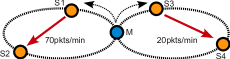
Figure 4.1: A simple network with two modes: The mobile can choose to orbit the left route or the right route. If it chooses the left (right) route, the mobile will come into contact with stationaries S1 and S2 (S3 and S4). On contact, the mobile can drop-off and pick-up data to and from the stationaries. In this figure, S1 generates a stream of data for S2 (S3 for S4). To serve the flow S1-S2, the mobile has to go into the left route, pick up data from S1 and drop them off to S2. If the flow S1-S2 has higher rate than S3-S4, the mobile should go into left route more often than right route.

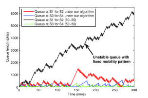
Figure 4.2: If the route operations percentages are set to 50-50 a priori, the source rates we have in Figure 4.1 can not be supported and will lead to unstable queues. However, as long as the source rates are in the capacity region (which takes into account the patrol requirements), our algorithm will support them and stabilize the queues.

4.2 Illustrative Example

Consider the simple network shown in Figure 4.1. We have one mobile that can choose from two “routes.” In the left route, it will come into contact with stationary nodes S1 and S2 (in that order); in the right route, with S3 and S4. On contact, the mobile can drop off and pick up data to and from the stationary nodes. Each route requires two minutes to finish, and after one route is finished, the mobile returns to the center and can choose the next route. On each contact, 200 packets can be picked up or dropped off by the mobile. In addition to transporting data between nodes, the mobile also has a purpose of patrolling the area, and must travel each route at least 15% of the time.

S1 generates data destined to S2 at a rate of 70pkts/min, and S3 generates data destined to S4 at a rate of 20pkts/min. The mobile does not know the data rates, and the rates can vary over time. If the mobility pattern of the mobile is fixed, then the network may not be able to support the two traffic flows. For example, if the mobile patrols each route 50% of the time, then the flow from S1 to S2 cannot be supported in the network and the queues are unstable, as shown in Figure 4.2.

In this dissertation, we develop an algorithm that controls the mobility pattern of the mobile dynamically so that it not only satisfies the surveillance requirement but also stabilizes the queues whenever it is possible. In the simple example in Figure 4.1, using our algorithm, the mobile may patrol the left route 75% of the time and the right route 25% so that each route is patrolled at least 15% of the time (surveillance requirement), and both traffic flows are supported and all queues are stable.

4.3 Related Works

The networks that utilize mobile carriers to transport data have been studied extensively recently by [24, 33, 79, 51, 27, 65, 16, 53, 43, 15, 8, 77, 74] and others. The primary focus of [65, 43, 74, 77] is to increase the data delivery probability and reduce delivery latency through replication in the context of delay-tolerant networks (DTN). Replication is useful in networks where mobile carriers move randomly because it increases the opportunities to transfer data from mobile nodes to static nodes and vice versa. In networks where the mobility patterns of mobiles are fixed, replication is not necessary. However, the drawback of fixed mobility patterns is that the network cannot dynamically respond to changes in the traffic loads. In addition, as long as data is delivered to the destination, it is considered sufficient, but in networks where the mobility pattern can be controlled, we can not only guarantee data delivery, but also the most efficient and optimal network resource utilization.

An extensive simulation study of a network where the mobile messengers are used to transport data among clusters has been done in [27]; there, the impact of different mobility patterns of the messengers on delay and efficiency is examined. In [18] and [70], algorithms that control the mobility of a mobile data collector in a sensor network to reduce data collection delay have been developed. Both papers explore the trade-off between mobility and wireless transmissions energy. In [20] a trajectory control algorithm such that the mobile data collector dynamically switches its trajectory to be closer to sensor nodes with more data to transmit in order to save TX power has been developed. In addition, [36, 61] explore sensor networks where nodes can reconfigure their positions dynamically in order to enhance coverage and life span. The work in [44] is a study of a routing protocol based on controlled mobility that minimizes the distance traveled by mobile carriers to reach the destination. However, the mobile messengers in [27, 18, 70, 20, 36, 44] cannot adapt their mobility patterns to traffic loads, the result of which will be unstable queues as illustrated in the previous section. Experimental evaluation of a heuristic mobility control algorithm that can respond to changing network capacity and demand is presented in [17]. Optimization based approaches for mobile data collection have been studied in [63], where the authors study the problem of mobile sinks that need to collect data from various sources before their respective buffers overflow. The algorithm based on using the deadlines (time to fill buffers at various nodes) is shown to be NP-complete, and various heuristics are then explored to alleviate this. Further, in [28], the authors study the problem of transporting data to a single collector from a collection of stationary data generators via reinforcement learning techniques.

The optimization framework based on back-pressure [73] that is used in our dissertation has been used extensively in [38, 22, 82, 68, 48, 52, 81, 50, 49] and many others for developing efficient resource allocation schemes in wired and wireless networks in the context of congestion control and back-pressure routing and rate control. The networks studied in these papers consist of static nodes, and the links are not intermittent, while in this dissertation, we focus on intermittently connected networks, and develop an algorithm that controls mobility to support network traffic flows while guaranteeing some other objectives such as surveillance requirement. The optimization algorithm that is most similar to ours is the one developed in [49]. The focus of [49] however is on an abstract problem of optimizing stochastic renewal systems; ours focuses on minimizing the cost of transporting data over mobile networks.

In this dissertation, we combine the optimization framework used for back-pressure routing with mobility control in order to develop a dynamic throughput and cost optimal mobility control algorithm that allows multiple mobiles to transport data among a collection of stationary nodes. Our contributions include:

1. We formulate a cost minimization framework for the network where the mobile carrier adapts its mobility pattern to support traffic flows among stationary nodes while satisfying a secondary surveillance objective. We present the min-cost mobility control algorithm that is throughput and cost optimal, and then develop a practical distributed algorithm.

2. We implement our practical distributed algorithm and present experimental results on our Pharos test bed [69] using the Click router [39], where we implement the radio and network aspects and emulate mobility.

4.4 Network Model

The network consists of $L$ stationary nodes and one mobile carrier. The stationary nodes do not move and can not communicate with each other directly; they must rely on the mobile carrier to transport data among them. We assume that stationary nodes generates data for other stationary nodes. Let $d_{l}$ denote the destination node of the data stream generated by stationary node $l$, and let $x_{l}^{d_{l}}$ (pkts/time slot) be the corresponding average rate. Let ${\bf{x}}=\left\{x_{l}^{d_{l}}\right\}$. Define

$$1_{\{l,l^{\prime}\}}=\left\{\begin{array}[]{ll}1&\text{ if }l^{\prime}=d_{l}\\ 0&\text{ else. }\end{array}\right.$$

A stationary node can exchange data with the mobile carrier when the two come into contact. During each contact, the mobile carrier can send $\eta_{d}$ packets to the stationary node, and receive $\eta_{p}$ packets from the stationary node. We call the transmissions from a stationary node to the mobile carrier a pick up, and the transmissions from the mobile carrier to a stationary node a drop off.

We assume that there is a terminal $V$ in the network. This terminal does not generate data. It is there to facilitate notation and understanding of the definition of route, which we define next.

Definition 1.

A route of the mobile carrier starts and ends at the terminal. The route is a (finite) set of tuples $(s,n_{s})$ where $s$ is a stationary node and $n_{s}$ is the number of times the mobile visits $s$ on that route. The route is further specified by the time required to patrol that route.  

Assumption 4.

We assume that there are $J$ routes for the mobile carrier, which are indexed by $j$. Stationary node $l$ is assessed a cost $a_{l,j}$ for every packet picked up by the mobile to be sent over route $j$ ($a_{l,j}$ is called pick up cost). The mobile incurs a cost of $b_{j}$ per time slot when patrolling route $j$.  

An example of a route is

$$R_{1}=\{(V,2),(l_{1},1),(l_{2},4),10mins\}.$$

On this route, the mobile starts at $V$, visits $l_{1}$ once and $l_{2}$ four times before returning to $V$. The time the mobile takes to patrol $R_{1}$ is 10mins. The route $R_{1}$ is different from the route $R_{2}=\{(V,2),(l_{1},2),(l_{2},4),10mins\}$ because $l_{1}$ is visited twice on $R_{2}$ but only once on $R_{1}$. $R_{1}$ is also different from the route $R_{3}=\{(V,2),(l_{1},1),(l_{2},4),5mins\}$ because it takes less time to patrol $R_{3}$. Note that the mobile carrier must return to the terminal before switching onto another route. Though not shown, the terminal in the network in Figure 4.1 would be located where the left and right routes meet (right under where the mobile is).

We can associate higher $b_{j}$ with the routes on which the mobile moves faster since that would require more fuel. We assume that $a_{l,j}\leq a_{\max},~{}\forall l,j$ and $b_{j}\leq b_{\max},~{}\forall j$. We let $f_{j}$ denote the fraction of time the mobile carrier is on route $j,$ and $T_{j}$ denote the time required to patrol route $j$ (in units of time slots). Assume that $T_{\min}\leq T_{j}\leq T_{\max},~{}\forall j$. If $N$ routes have been patrolled, and out of the $N$ routes, the mobile patrolled route $j$ $N_{j}$ times, then $f_{j}=\frac{N_{j}T_{j}}{\sum_{j^{\prime}}N_{j^{\prime}}T_{j^{\prime}}}$. Note that not all stationary nodes may be included on one route, so the mobile may have to switch from one route to another to transport packets from a source to its destination.

Definition 1 specifies a route of a mobile via the the collection of stationary nodes that a mobile visits, the number of times that each of them is visited, and the total time taken to physically traverse this route. Note that several physical paths (i.e., the actual geographic paths) can share the same mobile route as specified by this description (e.g., the difference between two physical paths could be the order in which the stationary nodes are visited, or that the actual trajectory could be different; however, the path characteristics are summarized by Definition 1 could be the same). In this case, multiple physical paths would be mapped to the same route. The reason for our choice of these parameters to define a route is that the list of stationary nodes along with the number of times that they are visited describe the transfer capacity between the mobile and stationary nodes, and this along with the time duration of the mobile route is needed to describe the rate of data transfer between the mobile and stationary nodes (rate = (number of contacts)$\times$(packets transferred per contact) $/$ (time duration of mobile route), see Table 4.1). Different physical paths with the same route parameters in Definition 1 lead to the same data transfer constraints, hence we do not distinguish between them (as the rest of the physical route properties are not relevant to our model for data transfer), and our algorithm will treat them all as the same route.

Note that if for some reason, we need to distinguish between physical paths that have the same route (e.g., with different costs), it is easy to do so by one of two means: (i) simply change the original route time durations (T, which is originally the same for the two routes) to be $(T-\epsilon)$ and $(T+\epsilon)$, for some arbitrarily small $\epsilon$; or (ii) augment the notation in Definition 1 to have an additional route-index parameter (that distinguishes between the two physical paths). All that this will change is to add an extra route queue in the Min-Cost Mobility Control Algorithm (see Section 4.5), and the algorithm will proceed to load-balance between these two routes based on the costs.

Surveillance Requirement: The mobile must periodically patrol route $j$ to guarantee that $f_{j}\geq p_{j}$ for some $p_{j}\geq 0$, $\forall~{}j$.  

We let $\zeta_{l,j}$ denote the number of contacts that can be made between the mobile carrier and stationary node $l$ on route $j$. Let $P_{l,j}$ and $D_{l,j}$ denote the rates that the mobile can receive from and transmit to node $l$ on route $j,$ i.e., $P_{l,j}=\frac{\eta_{p}\zeta_{l,j}}{T_{j}}$ and $D_{l,j}=\frac{\eta_{d}\zeta_{l,j}}{T_{j}}$.

Each stationary node $l$ maintains a queue $q_{l,j}$ for each route $j$, $j=1,...,J.$ Node $l$ deposits into queue $q_{l,j}$ the packets it wants the mobile to pick up on route $j$. The mobile maintains a queue $Q_{l^{\prime}}$ for each destination node $l^{\prime}$, $l^{\prime}=1,...,L$.

Definition 2.

We say the network is stable if all queues are bounded.  

We let

$$1_{\{P_{l,j}>0\}}=\left\{\begin{array}[]{ll}1&\text{ $P_{l,j}>0$}\\ 0&\text{ else. }\end{array}\right.$$

Finally, we define

$$\eta_{\max}=\max\left\{\max_{l,j}\left\{P_{l,j}T_{j}\right\},\max_{l,j}\left\{D_{l,j}T_{j}\right\}\right\}.$$

Notation	Description
$x_{l}^{d_{l}}$	rate stationary $l$ generates data for stationary $d_{l}$
$y_{l,j}^{d_{l}}$	rate mobile picks up data from $l$ on route $j$, destined for $d_{l}$
$p_{j}$ ($f_{j}$)	minimum (actual) fraction of time mobile spends on route $j$
$T_{j}$	time duration of mobile route $j$
$a_{l,j}$	cost $l$ pays to have a packet picked up on route $j$
$b_{j}$	cost per unit time mobile pays to spend on route $j$
$q_{l,j}$	queue $l$ maintains for packets to be picked on route $j$
$Q_{l}$	queue mobile maintains for packets destined for $l$
$\delta_{l,j}$	fraction of total resource on route $j$ stationary $l$ uses
$w_{j}$	counter mobile uses to satisfy the surveillance req. (4.5)
$K$	tuning param. that controls optimality and queue sizes
$\kappa$	tuning parameter that controls the size of the counter $w_{j}$
$\eta_{P}$	# of packets picked up per contact
$\eta_{D}$	# of packets dropped off per contact
$\zeta_{l,j}$	# of contacts mobile makes with $l$ on route $j$
$P_{l,j}$	data pick-up rate from $l$ on route $j$ ($\eta_{P}\zeta_{l,j}/T_{j}$)
$D_{l,j}$	data drop-off rate to $l$ on route $j$ ($\eta_{D}\zeta_{l,j}/T_{j}$)

Table 4.1: Description of variables used

4.5 Min-Cost Mobility Control

In this section, we will introduce our min-cost mobility control algorithm. The variables associated with our algorithm along with their brief physical description are given in Table 4.1. Define $y_{l,j}^{d_{l}}$ to be the (average, long-term) rate at which data generated by stationary node $l$ is picked up by the mobile carrier when patrolling route $j$. The objective of the min-cost mobility control is to find $\mathbf{f}=\{f_{j},j=1,...,J\}$ and $\mathbf{y}=\{y_{l,j}^{d_{l}},l=1,...,N,j=1,...,J\}$ (pick up rate splitting) to (i) stabilize the network, i.e., guarantee that the queue lengths are bounded, (ii) minimize the average cost $\sum_{l,j}y_{l,j}^{d_{l}}a_{l,j}+\sum_{j}b_{j}f_{j}$, and (iii) satisfy the surveillance requirement. These decisions are determined adaptively via a dual-decomposition inspired mobility control algorithm.

Definition 3.

We say the arrival rate $\mathbf{x}$ is supportable if there exists $(\mathbf{f},\mathbf{y})$ such that:

$$\sum_{j}y_{l,j}^{d_{l}} = x_{l}^{d_{l}}$$ (4.3)

$$\sum_{j}f_{j} \leq 1$$ (4.4)

$$f_{j} \geq p_{j}\in[0,1],~{}j=1,...,J$$ (4.5)

$$y_{l,j}^{d_{l}} = \delta_{l,j}f_{j}P_{l,j},~{}\forall l,j$$ (4.6)

$$\sum_{j,l}1_{\{l,l^{\prime}\}}\delta_{l,j}f_{j}P_{l,j} \leq \sum_{j}f_{j}D_{l^{\prime},j},~{}\forall l^{\prime}$$ (4.7)

$$0\leq \delta_{l,j} \leq 1.$$ (4.8)

 

Let $\Lambda$ be the set of all supportable arrival rates. Given $\mathbf{x}\in\Lambda$, let $\Gamma_{\mathbf{x}}$ denote the set of $(\mathbf{f},\mathbf{y})$ that satisfy the equations in definition 3. An arrival rate $\mathbf{x}$ is said to be supportable if there exist $\mathbf{f}$ and $\mathbf{y}$ such that: (i) The summation of $f_{j}$ (the fraction of time a mobile spends on route $j$) is less than one (eq. (4.4)) and the surveillance requirement (eq. (4.5)) is satisfied; (ii) The rate at which packets are transmitted from stationary node $l$ to the mobile while it is patrolling route $j$ is upper bounded by the pick up rate by the mobile on route $j$ (eq. (4.6)); (iii) The rate at which the data for destination node $l^{\prime}$ is picked up from all stationary nodes and on all routes is limited by the combined rate at which data is dropped off to node $l^{\prime}$ on all routes (eq. (4.7)). The parameter $\delta_{l,j}$ controls the fraction of active contacts between node $l$ and the mobile on route $j$; when the mobile and stationary node $l$ come into contact, they have the option of using only part, if any, of the transfer capacity of the contact; and (iv) The total rate the data is picked up from node $l$ on all routes should be equal to the rate at which node $l$ generates data (eq. (4.3)).

Note that we cannot replace conditions (4.6) and (4.7) with

$$y_{l,j}^{d_{l}}\leq f_{j}P_{l,j},~{}~{}~{}~{}~{}~{}~{}~{}~{}~{}~{}~{}~{}$$ (4.9)

$$\sum_{j,l}1_{\{l,l^{\prime}\}}f_{j}P_{l,j}\leq\sum_{j}f_{j}D_{l^{\prime},j}.$$ (4.10)

Consider two sources $s_{1}$ and $s_{2}$, with destinations $d_{1}$ and $d_{2}$, respectively. Assume that $s_{1}$ and $s_{2}$ can be visited by the mobile only when the mobile is on route $R_{0}$, and $x_{s_{1}}^{d_{1}}>x_{s_{2}}^{d_{2}}$. Suppose the pick-up rates from $s_{1}$ and $s_{2}$ are the same ($P_{s_{1},R_{0}}=P_{s_{2},R_{0}}$). Then if we enforce constraint (4.9), then $x_{s_{1}}^{d_{1}}=y_{s_{1},R_{0}}^{d_{1}}\leq f_{R_{0}}P_{s_{1},R_{0}}$ and $x_{s_{2}}^{d_{2}}=y_{s_{2},R_{0}}^{d_{2}}\leq f_{R_{0}}P_{s_{2},R_{0}}=f_{R_{0}}P_{s_{1},R_{0}}$. Assume that $d_{1}$ and $d_{2}$ are contacted by the mobile only when it is on routes $R_{1}$ and $R_{2}$, respectively, and they are receiving data only from $s_{1}$ and $s_{2}$, respectively. In addition, suppose that the drop-off rates to $d_{1}$ and $d_{2}$ are the same ($D_{d_{1},R_{1}}=D_{d_{2},R_{2}}$). If we force constraint (4.10), then $f_{R_{0}}P_{s_{1},R_{0}}\leq f_{R_{1}}D_{d_{1},R_{1}}$ and $f_{R_{0}}P_{s_{1},R_{0}}=f_{R_{0}}P_{s_{2},R_{0}}\leq f_{R_{2}}D_{d_{2},R_{2}}$ which implies that the mobile has to spend just as much time on $R_{2}$ as $R_{1}$, even though $x_{s_{1}}^{d_{1}}>x_{s_{2}}^{d_{2}}$. We resolve this issue by using $\delta_{l,j}$.

The objective of the minimum-cost mobility control is to solve the following optimization problem: Given $\mathbf{x}\in\Lambda$ and for any fixed $K>0,$

$$\text{minimize}\left\{K\sum_{l,j}y_{l,j}^{d_{l}}a_{l,j}+K\sum_{j}f_{j}b_{j}\right\}$$ (4.11)

$$\hbox{subject to }(\mathbf{f},\mathbf{y})\in\Gamma_{\mathbf{x}}.~{}~{}~{}~{}~{}~{}~{}~{}~{}~{}~{}~{}~{}~{}~{}~{}~{}$$

Let $\left(\mathbf{\hat{f}},\mathbf{\hat{y}}\right)$ denote an optimal solution to (4.11).

As we will see later, by suitably choosing the value of parameter $K>0$ in the optimization problem, the solution generated by our algorithm will be sufficiently “close” to the optimal. Next, note that multiplying both sides of constraint (4.5) by any positive constant $\kappa>0$ does not change the condition. Thus, the partial Lagrange dual of the optimization problem (4.11) is the following:

$$L(q_{l,j},Q_{l^{\prime}},w_{j})=$$

$$\min_{y_{l,j}^{d_{l}},f_{j},\delta_{l,j}}\left\{K\sum_{l,j}y_{l,j}^{d_{l}}a_{l,j}-\sum_{l,j}q_{l,j}\left(\delta_{l,j}f_{j}P_{l,j}-y_{l,j}^{d_{l}}\right)\right.$$

$$\left.-\sum_{l^{\prime}}Q_{l^{\prime}}\left(\sum_{j}f_{j}D_{l^{\prime},j}-\sum_{j,l}1_{\{l,l^{\prime}\}}\delta_{l,j}f_{j}P_{l,j}\right)\right.$$

$$\left.+K\sum_{j}f_{j}b_{j}-\sum_{j}\kappa w_{j}\left(f_{j}-p_{j}\right)\right\}$$

subject to 1) $\sum_{j}y_{l.j}^{d_{l}}=x_{l}^{d_{l}}$, 2) $\sum_{j}f_{j}\leq 1$, and 3) $\delta_{l,j}\in[0,1]$. As we will see later, the parameter $\kappa$ is useful in our algorithm in order to match the time-scale of route selection with the time-scale of queue-length variation.

We now observe that we can decompose the Lagrange dual into two subproblems:

$$\min_{y_{l,j}^{d_{l}}\geq 0} K\sum_{j}y_{l,j}^{d_{l}}a_{l,j}+\sum_{j}q_{l,j}y_{l,j}^{d_{l}}$$ (4.12)

s.t. $$\sum_{j}y_{l,j}^{d_{l}}=x_{l}^{d_{l}}$$

for each $l=1,...,L$ and

$$\max_{f_{j}\geq 0,\delta_{l,j}} \sum_{l,j}q_{l,j}\delta_{l,j}f_{j}P_{l,j}+\sum_{j}\kappa w_{j}\left(f_{j}-p_{j}\right)$$

$$+\sum_{l^{\prime},j}Q_{l^{\prime}}f_{j}\left(D_{l^{\prime},j}-\sum_{l}1_{\{l,l^{\prime}\}}\delta_{l,j}P_{l,j}\right)$$

$$-K\sum_{j}f_{j}b_{j}$$

s.t. $$\sum_{j}f_{j}\leq 1\text{ and }\delta_{l,j}\in[0,1]~{}\forall~{}l,j~{}~{}~{}~{}~{}~{}~{}~{}$$

Motivated by the dual decomposition, we propose the following min-cost mobility control algorithm. Here, the index $k$ denotes the $k$-th route selection. If the $k$-th route is $j$, the time duration between $k$-th and $(k+1)$-th route selections is $T_{j}$. In the min-cost mobility control algorithm, a stationary node deposits its packets into a queue that solves the subproblem (4.12), and a mobile station selects its route by solving subproblem (4.5). In addition to packet queues, each mobile station maintains a deficit counter for each route. The size of a deficit counter indicates the number of times the mobile node needs to further patrol the route to fulfill the surveillance requirement.

  Min-Cost Mobility Control Algorithm

1. Stationary node $l$ deposits $y_{l,j}^{d_{l}}(k)$ packets into queue $q_{l,j},$ where

   $$y_{l,j}^{d_{l}}(k)=\left\{\begin{array}[]{ll}x_{l}^{d_{l}}&\text{ if }j=j_{l}^{*}(k)\\ 0&\text{ else, }\end{array}\right.$$ (4.16)

   and $j_{l}^{*}(k)=\operatorname*{arg\,min}_{j}\left\{Ka_{l,j}+q_{l,j}(k)\right\}$.

2. The $k$-th route $j^{*}(k)$ selected by the mobile carrier is such that

   $$j^{*}(k)\in\arg\max_{j}\left\{\sum_{l}q_{l,j}(k)\delta_{l,j}(k)P_{l,j}-Kb_{j}\right.$$

   $$\left.+\sum_{l^{\prime}}Q_{l^{\prime}}(k)\left(D_{l^{\prime},j}-\sum_{l}1_{\{l,l^{\prime}\}}\delta_{l,j}(k)P_{l,j}\right)\right.$$

   $$\left.+\kappa w_{j}(k)(1-p_{j})\right\}~{}~{}~{}~{}~{}~{}~{}~{}~{}~{}~{}~{}~{}~{}~{}~{}~{}~{}~{}~{}~{}~{}~{}~{}~{}~{}~{}~{}~{}~{}~{}$$ (4.17)

   where

   $$\delta_{l,j}(k)=$$ (4.18)

   $$\left\{\begin{array}[]{ll}1&\text{ if }1_{\{P_{l,j}>0\}}\left[q_{l,j}(k)-\sum_{l^{\prime}}1_{\{l,l^{\prime}\}}Q_{l^{\prime}}(k)\right]>0\\ 0&\text{ else. }\end{array}\right.$$ (4.20)

   The mobile will pick up data from $l$ on route $j^{*}(k)$ if and only if $\delta_{l,j^{*}(k)}(k)=1$. In addition,

   $$f_{j}(k)=\left\{\begin{array}[]{ll}1&\text{ if }j=j^{*}(k)\\ 0&\text{ else, }\end{array}\right.$$ (4.23)

   and

   $$T(k)=T_{j^{*}(k)}.$$ (4.24)

3. The queues are updated as follows:

   $$q_{l,j}(k+1)=\left[q_{l,j}(k)+~{}~{}~{}~{}~{}~{}~{}~{}~{}~{}~{}~{}~{}~{}~{}~{}\right.$$

   $$\left.T(k)\left(y_{l,j}^{d_{l}}(k)-\delta_{l,j}(k)P_{l,j}1_{\{f_{j}(k)=1\}}\right)\right]^{+}$$ (4.25)

   $$Q_{l^{\prime}}(k+1)=\left[Q_{l^{\prime}}(k)+\sum_{j}1_{\{f_{j}(k)=1\}}T(k)\right.$$

   $$\left.\times\left[\sum_{l}1_{\{l,l^{\prime}\}}\delta_{l,j}(k)P_{l,j}-D_{l^{\prime},j}\right]\right]^{+}$$ (4.26)

4. The algorithm maintains a deficit counter $w_{j}(k)$ for route $j$ such that at step $k$, $w_{j}(k)$ is increases by $T(k)p_{j}$ and decreases by $T(k)f_{j}(k)$, i.e.,

   $$w_{j}(k+1)=\left[w_{j}(k)+T(k)p_{j}-1_{\{f_{j}(k)=1\}}T(k)\right]^{+}.$$ (4.27)

 

The next two theorems demonstrate the stability and optimality of our proposed algorithm, respectively.

Theorem 3.

Given $\mathbf{x}$ such that $(1+\epsilon)\mathbf{x}\in\Lambda$ for some $\epsilon>0$, under the iterative algorithm above, the network is stable.

Proof: See Appendix A.  

Theorem 4.

Given $\mathbf{x}$ such that $(1+\epsilon)\mathbf{x}\in\Lambda$ for some $\epsilon>0$, let $\left\{\hat{f}_{j},\hat{y}_{l,j}^{d_{l}}\right\}$ be the solution to the optimization problem (4.11). As $K\rightarrow\infty$, under our proposed algorithm,

$$\sum_{l,j}a_{l,j}\hat{y}_{l,j}^{d_{l}}+\sum_{j}\hat{f}_{j}b_{j}=\lim_{K\rightarrow\infty}\lim_{k^{\prime}\rightarrow\infty}\left[\frac{1}{\sum_{k\leq k^{\prime}}T(k)}\right.$$

$$\left.\times\left(\sum_{k\leq k^{\prime}}\left(\sum_{l,j}T(k)a_{l,j}y_{l,j}^{d_{l}}(k)+\sum_{j}f_{j}(k)T(k)b_{j}\right)\right)\right].$$ (4.28)

Proof: See Appendix B.  

Note that $\lim_{k^{\prime}\rightarrow\infty}\frac{1}{\sum_{k\leq k^{\prime}}T(k)}\sum_{k\leq k^{\prime}}T(k)y_{l,j}^{d_{l}}(k)$ in equation (4.28) is the time-average data rate that the mobile picks up from stationary node $l$ on route $j$, and $\lim_{k^{\prime}\rightarrow\infty}\frac{1}{\sum_{k\leq k^{\prime}}T(k)}\sum_{k\leq k^{\prime}}T(k)f_{j}(k)$ is the fraction of the time the mobile patrols route $j$.

4.5.1 Impact of $K$ and $\kappa$

We know from [50] that $(\mathbf{f},\mathbf{y})$ obtained by our algorithm is within a factor of $O(1/K)$ from $(\mathbf{\hat{f}},\mathbf{\hat{y}})$, and while $q_{l,j}$, $Q_{l^{\prime}}$ and $\kappa w_{j}$ are $O(K\max\{\eta_{\max},\kappa T_{\max}\})$, where $\max\{\eta_{\max},\kappa T_{\max}\}$ is the maximum amount by which $q_{l,j}$, $Q_{l^{\prime}}$, and $\kappa w_{j}$ can increase between any two consecutive route selections. In order to keep $q_{l,j}$ and $Q_{l^{\prime}}$ small and make the mobile go into “surveillance” route without having $w_{j}$ build up, we choose $\kappa$ such that $\eta_{\max}\approx\kappa T_{\max}$, i.e. $\kappa=\Theta\left(\eta_{max}/T_{\max}\right)$.

4.5.2 Multiple Mobiles

So far, our model assumes only one mobile node to keep notation simple. However, one can easily extend the algorithm to a network with multiple mobiles. A straightforward way to extend our model is to have the stationary nodes maintain a queue for each route and each mobile, i.e., stationary node $l$ maintains a queue $q_{l,j,m}$ for route $j$ for mobile $m$. Let $f_{m,j}$ denote the fraction of time mobile $m$ operates on route $j$. We then have the constraint $\sum_{j\in M_{m}}f_{m,j}\leq 1$ for each mobile $m$, where $M_{m}$ is the set of routes mobile $m$ can patrol. Each mobile also has its own “surveillance” or secondary objective constraints on $f_{m,j}$. Finally, each mobile solves the optimization problem (4.5) independently, without any cooperation with other mobiles.

It is easy to show that the results in this dissertation immediately carry over to this more general setting (the proofs are analogous to those presented here). Lastly, we note that this more general formulation supports multiple terminals, so that different mobiles can return to different terminal after each patrol.

4.6 Practical Algorithm

The min-cost mobility control algorithm we discussed in the previous section has two shortcomings. One is that the source nodes have to synchronize their queue selections with the mobile’s selection. The second issue is that the mobile has to know $q_{l,j}$’s to make the route selection. However, we can take advantage of the secondary surveillance objective of the mobile. While the mobile makes its surveillance round, it can collect the most up-to-date queue information while picking up and dropping off data, and use the information in selecting the next route.

Let $k$ denote the $k^{\text{th}}$ route the mobile operates on. We can recast the update equations (4.16), (4.17) and (4.18) into the following practical, distributed decision controls.

Stationary node: The first time the mobile contacts stationary node $l$, it communicates the values of $a_{l,j}$’s corresponding only to the routes on which it will visit stationary node $l$. For each new packet, the stationary node $l$ computes

$$j_{l}^{*}=\operatorname*{arg\,min}_{j}Ka_{l,j}+q_{l,j}$$ (4.29)

and deposits it into $q_{l,j_{l}^{*}}$.

Mobile: Each time the mobile meets stationary node $l$, it collects all queue size information from node $l$ at the end of the contact. At the end of the execution of a route, the mobile computes the next route $f_{j},\delta_{l,j}\in\{0,1\}$ by maximizing

$$\sum_{l\in j}{\bf q_{l,j}}\delta_{l,j}f_{j}P_{l,j}+\sum_{l^{\prime}\in j}Q_{l^{\prime}}f_{j}\left(D_{l^{\prime},j}-\delta_{l,j}P_{l,j}\right)$$

$$+\sum_{j}\kappa w_{j}\left(f_{j}-p_{j}\right)-K\sum_{j}f_{j}b_{j}~{}~{}~{}~{}~{}~{}~{}$$ (4.30)

where ${\bf q_{l,j}}$ denotes the most up-to-date information known to the mobile.

4.7 Experimental Results

We implemented the practical version of our algorithm as described in Section 4.6 in Click [39] on our testbed [69] (see also [59] for more details). The purpose of the experiment is to demonstrate that our practical algorithm can achieve the optimal value and to show that we can come arbitrarily close to the optimal value at the expense of longer queues as $K\rightarrow\infty$. The algorithm presented in Section 4.5 assumes perfect knowledge of the queue length by the mobile, while the practical version does not. To this end, we build our experimental network with WiFi cards on the Proteus platform [69]. We emulate the mobility by timed contacts, i.e., the mobile node is, in our emulation, stationary, and would make contact with one static node, then wait for some time before making contact with another static node. These timed contacts are implemented simply by turning on and off the appropriate wireless interfaces for the various nodes.

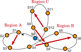
Figure 4.3: A network with one mobile and 12 stationaries, 4 in each region. The mobile has two modes per region: a fast and a slow route. In fast route, the mobile goes through a region and comes back to the center in one minute; in slow route, it takes two minutes. All stationaries in the region are contacted in each route. (The terminal would be located where the three regions meet.)

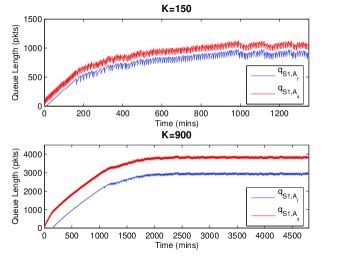
Figure 4.4: Queue lengths observed at S1: Increasing $K$ results in more optimal rate allocations, but it comes at the price of longer queues and longer time for convergence.

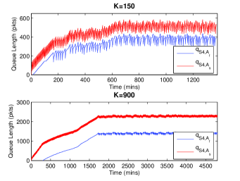
Figure 4.5: Queue lengths observed at S4

4.7.1 Experiment 1

The network we used in this experiment is shown in Figure 4.1. We use the following routes:

$$R_{1} = \{(V,2),(S1,1),(S2,1),1min\}$$

$$R_{2} = \{(V,2),(S1,1),(S2,1),2mins\}$$

$$R_{3} = \{(V,2),(S3,1),(S4,1),1min\}$$

$$R_{4} = \{(V,2),(S3,1),(S4,1),2mins\}$$

We used two flows, one from S1 to S2, at the rate of 40pkts/min and another one from S2 to S3 at the rate of 30pkts/min. The mobile and the nodes can transmit 100pkts per contact. The routes $R_{2}$ and $R_{4}$ must be patrolled at least 10% of the time, i.e., $p_{2}=p_{4}=0.1$ and $p_{1}=p_{3}=0$. $a_{S1,R_{1}}=a_{S2,R_{1}}=K$ and $a_{S1,R_{2}}=a_{S2,R_{2}}=0$; $b_{R_{1}}=b_{R_{3}}=K$ and $b_{R_{2}}=b_{R_{4}}=0$. The rate splitting over the modes $x_{S1,0}^{S2}$ and $x_{S1,1}^{S2}$ is shown in Table 4.2. (The optimal values in Tables 4.2 and 4.3 are obtained by numerically solving the optimization problem (4.11) using MATLAB.)

	$K$
	150	300	600	Optimal
$y_{S1,R_{1}}^{S2}$	20	18.376	15.8	15
$y_{S1,R_{2}}^{S2}$	20	21.624	24.2	25
$y_{S2,R_{1}}^{S3}$	9.9	8.598	5.97	5
$y_{S2,R_{2}}^{S3}$	20.1	21.402	24.03	25

Table 4.2: Experiment 1: The mobile has to travel the left routes $R_{1}$ and $R_{2}$ to pick up data from S2 and travel the right routes $R_{3}$ and $R_{4}$ to drop off data to S3. The mobile must patrol routes $R_{2}$ and $R_{4}$ at least 10% of the time to satisfy the surveillance requirement. The stationary nodes and the mobile will try to utilize the “cheaper” routes $R_{2}$ and $R_{4}$ (thus, more packets are picked up on those routes) before the more costly routes $R_{1}$ and $R_{3}$. (The units are pkts/min.)

4.7.2 Experiment 2

In this experiment, we used the network shown in Figure 4.3. The network is composed of three regions, A, B, and C. In each region, the mobile has two routes, fast and slow. We use $A_{f}$ and $A_{s}$ to denote the fast and slow routes in region A, respectively. ($B_{f}$ and $B_{s}$ for region B and $C_{f}$ and $C_{s}$ for region C.) On a fast route, the mobile goes through the region in one minute; on slow a route, the mobile takes two minutes. Each stationary node in a region is contacted once on each route made through that region.

On each route, the mobile makes contacts starting from the lowest numbered stationary to the highest. Each slow route is required to be patrolled at least 10% of the time, i.e., $p_{A_{s}}=p_{B_{s}}=p_{C_{s}}=0.1$. On each contact, the mobile can pick up and drop off 100pkts (200pkts total).

S1 generates data for S3 at rate 23pkts/min; S4 generates data for S6 at 20pkts/min. S9 generates data for S8 at rate 20pkts/min, and S12 generates data for S10 at rate 23pkts/min. The packet pick up costs $a_{l,A_{s}}$, $a_{l,B_{s}}$, and $a_{l,C_{s}}$ for the slow route are 0 for all stationary nodes; the pick up costs $a_{l,A_{f}}$, $a_{l,B_{f}}$ and $a_{l,C_{f}}$ for the fast route are $K$. The route costs are $b_{A_{s}}=b_{B_{s}}=b_{C_{s}}=0$ and $b_{A_{f}}=b_{B_{f}}=b_{C_{f}}=K$. We let $K=150$, $450$, and $900$. $\kappa$ is set to 100.

We compute the optimal rate splitting by solving the optimization problem (4.11) (shown in the “Optimal” column) and compare against the observed rate splitting under different values of $K$. As predicted by Theorem 4, the rate allocation approaches the optimal allocation as $K$ increases as shown in Table 4.3. The price of being close to the optimal rates is long queues, as demonstrated in Figures 4.4 and 4.5 for $K=150$ and $900$.

	$K$
$y_{l,j}^{d_{l}}$	150	450	900	Optimal
$y_{S1,A_{f}}^{S3}$	10.488	9.5	8.51	8.5
$y_{S1,A_{s}}^{S3}$	12.512	13.5	14.49	14.5
$y_{S4,A_{f}}^{S6}$	7.6	6.172	5.4	5.5
$y_{S4,A_{s}}^{S6}$	12.4	13.828	14.6	14.5
$y_{S9,C_{f}}^{S8}$	7.64	6.112	5.378	5.5
$y_{S9,C_{s}}^{S8}$	12.36	13.888	14.622	14.5
$y_{S12,C_{f}}^{S10}$	10.78	9.33	8.372	8.5
$y_{S12,C_{s}}^{S10}$	12.22	13.67	14.628	14.5

Table 4.3: Experiment 2: As $K$ increases, the rate splitting approaches the optimal. (The units are pkts/min.)

Appendix A: Proof of Theorem 3

Consider the Lyapunov function $V(k)=\sum_{l,j}\left(q_{l,j}(k)\right)^{2}+\sum_{l^{\prime}}\left(Q_{l^{\prime}}(k)\right)^{2}+\kappa\sum_{j}\left(w_{j}(k)\right)^{2}$. Define $\Delta V(k)=V(k+1)-V(k)$. Note that

$$\Delta V(k) \leq \sum_{l,j}\left(q_{l,j}(k+1)-q_{l,j}(k)\right)\left(2q_{l,j}(k)+\eta_{\max}\right)$$

$$+\sum_{l^{\prime}}\left(Q_{l^{\prime}}(k+1)-Q_{l^{\prime}}(k)\right)\left(2Q_{l^{\prime}}(k)+\eta_{\max}\right)$$

$$+\kappa\sum_{j}\left(w_{j}(k+1)-w_{j}(k)\right)\left(2w_{j}(k)+T_{\max}\right)$$

since $\left(q_{l,j}(k+1)\right)^{2}-\left(q_{l,j}(k)\right)^{2}=\left(q_{l,j}(k+1)+q_{l,j}(k)\right)\left(q_{l,j}(k+1)-q_{l,j}(k)\right)$ and $\left(q_{l,j}(k+1)+q_{l,j}(k)\right)\leq 2q_{l,j}(k)+\eta_{\max}$. (Likewise for $Q_{l^{\prime}}(k)$ and $w_{j}(k)$.) The maximum amount by which $q_{l,j}(k)$ and $Q_{l^{\prime}}(k)$ can increase in one iteration is $\eta_{\max}$; the maximum amount by which $w_{j}(k)$ can increase in one iteration is $T_{\max}$.

We prove that there exists $q_{\max}$ such that if $q_{l,j}(k)$ or $Q_{l^{\prime}}(k)>q_{\max}$ for some $l$, $j$, $l^{\prime}$, and $k$, then

$$\Delta V(k)<-\alpha$$ (4.32)

where $\alpha>0$. Equation (4.32) would prove the evolution of $\left\{q_{l,j}(k),Q_{l^{\prime}}(k)\right\}$ is upper bounded.

Define:

$$\tilde{q}_{l,j}(k) = \max\left\{T(k)\delta_{l,j}(k)f_{j}(k)P_{l,j}-q_{l,j}(k),0\right\}$$ (4.33)

$$\tilde{Q}_{l^{\prime}}(k) = \max\left\{T(k)\sum_{j}f_{j}(k)D_{l^{\prime},j}-Q_{l^{\prime}}(k),0\right\}$$ (4.34)

$$\tilde{w}_{j}(k) = \max\left\{T(k)-w_{j}(k),0\right\}.$$ (4.35)

Note that if $q_{l,j}(k)\geq\eta_{\max}$ and $Q_{l^{\prime}}(k)\geq\eta_{\max}$, then $\tilde{q}_{l,j}(k)=0$ and $\tilde{Q}_{l^{\prime}}(k)=0$, respectively, and if $w_{j}(k)\geq T_{\max}$, then $\tilde{w}_{j}(k)=0$.

Using equations (4.25), (4.26), (4.27) (4.33), (4.34), and (4.35), the Lyapunov down drift equation (4) can be bounded as

$$\Delta V(k) \leq 2\sum_{l,j}\left[T(k)\left(y_{l,j}^{d_{l}}(k)-\delta_{l,j}(k)f_{j}(k)P_{l,j}\right)+\tilde{q}_{l,j}(k)\right]q_{l,j}(k)$$

$$+2\sum_{l^{\prime}}\left[f_{j}(k)T(k)\left(\sum_{l}1_{\{l,l^{\prime}\}}\delta_{l,j}(k)P_{l,j}-D_{l^{\prime},j}\right)+\tilde{Q}_{l^{\prime}}(k)\right]Q_{l^{\prime}}(k)$$

$$+2\kappa\sum_{j}\left(T(k)p_{j}-T(k)f_{j}(k)+\tilde{w}_{j}(k)\right)w_{j}(k)$$

$$+2\sum_{l,j}\eta_{\max}^{2}+2\sum_{l^{\prime}}\eta_{\max}^{2}+2\kappa\sum_{j}T_{\max}^{2}$$

because 1) $q_{l,j}(k+1)-q_{l,j}(k)\leq 2\eta_{\max}$, 2) $Q_{l^{\prime}}(k+1)-Q_{l^{\prime}}(k)\leq 2\eta_{\max}$, 3) $w_{j}(k+1)-w_{j}(k)\leq 2T_{\max}$, and 4)

$$q_{l,j}(k+1)-q_{l,j}(k)\leq$$

$$T(k)\left(y_{l,j}^{d_{l}}(k)-\delta_{l,j}(k)f_{j}(k)P_{l,j}\right)+\tilde{q}_{l,j}(k),$$

$$Q_{l^{\prime}}(k+1)-Q_{l^{\prime}}(k)\leq$$

$$f_{j}(k)T(k)\left(\sum_{l}1_{\{l,l^{\prime}\}}\delta_{l,j}(k)P_{l,j}-D_{l^{\prime}.j}\right)+\tilde{Q}_{l^{\prime}}(k),$$

and $w_{j}(k+1)-w_{j}(k)\leq T(k)\left(p_{j}-f_{j}(k)\right)+\tilde{w}_{j}(k)$.

Because of equations (4.33), (4.34) and (4.35), we have

$$\tilde{q}_{l,j}(k)q_{l,j}(k) \leq \eta_{\max}^{2}$$ (4.36)

$$\tilde{Q}_{l^{\prime}}(k)Q_{l^{\prime}}(k) \leq \eta_{\max}^{2}$$ (4.37)

$$\tilde{w}_{j}(k)w_{j}(k) \leq T_{\max}^{2}.$$ (4.38)

Let

$$A(k) = \sum_{l,j}y_{l,j}^{d_{l}}(k)q_{l,j}(k)$$ (4.39)

and

$$B(k) = \sum_{l,j}\delta_{l,j}(k)f_{j}(k)P_{l,j}q_{l,j}(k)$$ (4.40)

$$+\sum_{l^{\prime},j}f_{j}(k)Q_{l^{\prime}}(k)\left(D_{l^{\prime},j}-\sum_{l}1_{\{l,l^{\prime}\}}\delta_{l,j}(k)P_{l,j}\right).$$

Let

$$C = 2\sum_{l,j}\eta_{\max}^{2}+2\sum_{d_{l}}\eta_{\max}^{2}+2\kappa\sum_{j}T_{\max}^{2}.$$ (4.41)

Then,

$$\Delta V(k) \leq 2A(k)T(k)-2B(k)T(k)+2C$$ (4.42)

$$-2\kappa\sum_{j}T(k)(f_{j}(k)-p_{j})w_{j}(k)$$

due to equations (4.36), (4.37), (4.38), (4.39), (4.40), and (4.41).

Since $(1+\epsilon){\bf{x}}\in\Lambda$, there exist $\{\tilde{y}_{l,j}^{d_{l}}\}$, $\{\tilde{f}_{j}\}$, and $\{\tilde{\delta}_{l,j}\}$ in $\Gamma_{(1+\epsilon)\mathbf{x}}$ that satisfy the definition 3. Let

$$\tilde{B}(k) = \sum_{l,j}\tilde{\delta}_{l,j}\tilde{f}_{j}P_{l,j}q_{l,j}(k)$$ (4.43)

$$+\sum_{l^{\prime},j}\tilde{f}_{j}Q_{l^{\prime}}(k)\left(D_{l^{\prime},j}-\sum_{l}1_{\{l,l^{\prime}\}}\tilde{\delta}_{l,j}P_{l,j}\right).~{}~{}~{}$$

Then,

$$\Delta V(k) \leq 2T(k)\left[A(k)-\left(B(k)-\tilde{B}(k)+\tilde{B}(k)\right)\right.$$

$$\left.-\kappa\sum_{j}(f_{j}(k)-p_{j})w_{j}(k)\right]+2C.$$

To the RHS of the above inequality, we add and subtract the following two terms 1) $2K\sum_{j}f_{j}(k)b_{j}T(k)$ 2) $2K\sum_{j}\tilde{f}_{j}b_{j}T(k)$ and add $2\kappa T(k)\sum_{j}\left(\tilde{f}_{j}-p_{j}\right)w_{j}(k)$ ($\geq 0$ since $\tilde{f}_{j}$ satisfies inequality (4.5)). Thus, we get

$$\Delta V(k) \leq 2T(k)\left[A(k)-\left(B(k)-\tilde{B}(k)+\tilde{B}(k)\right.\right.$$ (4.44)

$$\left.\left.-K\sum_{j}f_{j}(k)b_{j}+K\sum_{j}\tilde{f}_{j}b_{j}\right)-K\sum_{j}f_{j}(k)b_{j}\right.$$

$$\left.+K\sum_{j}\tilde{f}_{j}b_{j}-\kappa\sum_{j}(f_{j}(k)-p_{j})w_{j}(k)\right.$$

$$\left.+\kappa\sum_{j}\left(\tilde{f}_{j}-p_{j}\right)w_{j}(k)\right]+2C$$

$$\leq 2A(k)T(k)-2\tilde{B}(k)T(k)+2C$$

$$-2K\sum_{j}f_{j}(k)b_{j}T(k)+2K\sum_{j}\tilde{f}_{j}b_{j}T(k).$$

Inequality (4.44) holds because

$$B(k)-K\sum_{j}f_{j}(k)b_{j}+\kappa\sum_{j}(f_{j}(k)-p_{j})w_{j}(k)$$

$$\geq\tilde{B}(k)-K\sum_{j}\tilde{f}_{j}b_{j}+\kappa\sum_{j}\left(\tilde{f}_{j}-p_{j}\right)w_{j}(k)$$

by algorithms (4.17) and (4.18). Hence,

$$\Delta V(k) \leq 2A(k)T(k)-2\tilde{B}(k)T(k)+2C-2KT(k)\sum_{j}b_{j}\left(f_{j}(k)-\tilde{f}_{j}\right)$$ (4.46)

$$\leq 2T(k)\left[\sum_{l,j}y_{l,j}^{d_{l}}(k)q_{l,j}(k)-\sum_{l,fj}\tilde{\delta}_{l,j}\tilde{f}_{j}P_{l,j}q_{l,j}(k)\right.$$

$$\left.-K\sum_{j}b_{j}\left(f_{j}(k)-\tilde{f}_{j}\right)\right]+2C$$

$$\leq 2T(k)\left[\sum_{l,j}y_{l,j}^{d_{l}}(k)q_{l,j}(k)-2\sum_{l,j}\tilde{y}_{l,j}^{d_{l}}q_{l,j}(k)\right.$$

$$\left.-2K\sum_{j}b_{j}\left(f_{j}(k)-\tilde{f}_{j}\right)\right]+2C.$$

Equation (4.46) follows because $\{\tilde{f}_{j}\}$ and $\{\tilde{\delta}_{l,j}\}$ satisfy (4.7). Equation (4.46) follows because $\{\tilde{y}_{l,j}^{d_{l}}\}$ satisfies (4.6). Adding and subtracting

$$2K\sum_{l,j}a_{l,j}T(k)\left(\tilde{y}_{l,j}^{d_{l}}+y_{l,j}^{d_{l}}(k)\right)$$

to RHS of equation (4.46), we have

$$\Delta V(k) \leq 2\sum_{l,j}T(k)y_{l,j}^{d_{l}}(k)\left(Ka_{l,j}+q_{l,j}(k)\right)+2C$$ (4.47)

$$-2\sum_{l,j}T(k)\tilde{y}_{l,j}^{d_{l}}\left(Ka_{l,j}+q_{l,j}(k)\right)$$

$$-2K\sum_{l,j}a_{l,j}T(k)\left(y_{l,j}^{d_{l}}(k)-\tilde{y}_{l,j}^{d_{l}}\right)$$

$$-2KT(k)\sum_{j}b_{j}\left(f_{j}(k)-\tilde{f}_{j}\right).$$

Note that up until this point, we have only used the fact that $(1+\epsilon)\textbf{x}\in\Lambda$ (and various substitutions) to arrive at the upper bound (4.47). Because of algorithm (4.16), we have

$$\sum_{l,j}T(k)y_{l,j}^{d_{l}}(k)\left(Ka_{l,j}+q_{l,j}(k)\right)=$$

$$\sum_{l}x_{l}^{d_{l}}T(k)\min_{j}\left\{Ka_{l,j}+q_{l,j}(k)\right\}.$$ (4.48)

Since $\sum_{j}\tilde{y}_{l,j}^{d_{l}}=(1+\epsilon)x_{l}^{d_{l}}$,

$$(1+\epsilon)\sum_{l}x_{l}^{d_{l}}T(k)\min_{j}\left\{Ka_{l,j}+q_{l,j}(k)\right\}$$

$$\leq\sum_{l,j}T(k)\tilde{y}_{l,j}^{d_{l}}q_{l,j}(k)+K\sum_{l,j}a_{l,j}T(k)\tilde{y}_{l,j}^{d_{l}}.$$ (4.49)

Thus,

$$\Delta V(k) \leq 2C-2K\sum_{l,j}T(k)a_{l,j}\left(y_{l,j}^{d_{l}}(k)-\tilde{y}_{l,j}^{d_{l}}\right)$$

$$-2\epsilon\sum_{l}x_{l}^{d_{l}}T(k)\min_{j}\left\{q_{l,j}(k)+Ka_{l,j}\right\}$$

$$-2KT(k)\sum_{j}b_{j}\left(f_{j}(k)-\tilde{f}_{j}\right).$$

Since $a_{l,j}\leq a_{\max}$, $b_{j}\leq b_{\max}$, $T_{\min}\leq T_{j}\leq T_{\max}$, and $T(k)y_{l,j}^{d_{l}}(k),T(k)\tilde{y}_{l,j}^{d_{l}}\leq\eta_{\max}$, we have

$$q_{\max}^{\prime} = 2C+2K\sum_{l,j}\eta_{\max}+2K\sum_{j^{\prime}}b_{\max}T_{\max}$$

$$\geq 2C-2K\sum_{l,j}T(k)a_{l,j}\left(y_{l,j}^{d_{l}}(k)-\tilde{y}_{l,j}^{d_{l}}\right)$$

$$-2KT(k)\sum_{j}b_{j}\left(f_{j}(k)-\tilde{f}_{j}\right),$$

and

$$\Delta V(k) \leq q_{\max}^{\prime}-2\epsilon\sum_{l}x_{l}^{d_{l}}T(k)\min_{j}\left\{q_{l,j}(k)+Ka_{l,j}\right\}.$$

Let

$$\nu=\min\left\{x_{l}^{d_{l}}~{}s.t.~{}x_{l}^{d_{l}}>0\right\},$$

i.e., $\nu$ is the smallest source rate greater than 0 among all sources in the network . If there is $l$ such that $q_{l,j}(k)>q_{\max}=q_{\max}^{\prime}/(2\epsilon T_{\min}\nu)$ for all $j$, then equation (4.32) holds. Thus,

$$q_{l,j}(k)\leq q_{\max}+\eta_{\max},~{}\forall l,j,k.$$ (4.50)

The control decision in equation (4.18) combined with the bound (4.50) prevents $Q_{l^{\prime}}(k)$ from being $>q_{\max}+\eta_{\max}$ for any $l^{\prime},k$. Thus, $Q_{l^{\prime}}(k)\leq q_{\max}+\eta_{\max}$ $\forall l^{\prime},k$.

Because of equation (4.50), $A(k)T(k)\leq\sum_{l,j}\eta_{\max}q_{\max}$. By simply adding $2K\sum_{j}f_{j}(k)b_{j}T(k)>0$ to eq. (4.42), we have

$$\Delta V(k) \leq 2A(k)T(k)-2B(k)T(k)+2C$$

$$-2\kappa\sum_{j}T(k)(f_{j}(k)-p_{j})w_{j}(k)+2K\sum_{j}f_{j}(k)b_{j}T(k)$$

If there is $w_{j}(k)$ such that

$$w_{j}(k)>\frac{\sum_{l,j}\eta_{\max}q_{\max}+C+2\sum_{j}Kb_{\max}T_{\max}}{\kappa\left(1-p_{j}\right)T_{\min}},$$

then

$$B(k)T(k)+\kappa\sum_{j}T(k)\left(f_{j}(k)-p_{j}\right)w_{j}(k)-K\sum_{j}f_{j}(k)b_{j}T(k)$$

$$\geq\sum_{l,j}\eta_{\max}q_{\max}+C+K\sum_{j}b_{\max}T_{\max}~{}~{}~{}~{}~{}~{}~{}~{}~{}~{}~{}~{}~{}~{}~{}~{}~{}~{}~{}~{}~{}~{}~{}~{}~{}~{}$$

by algorithm (4.17), which implies that $\Delta V(k)<0$. Thus, if

$$w_{j}(k)>\frac{\sum_{l,j}\eta_{\max}q_{\max}+C+K\sum_{j}b_{\max}T_{\max}}{\kappa\left(1-p_{j}\right)T_{\min}}$$

for some $j,k$, then $\Delta V(k)$ satisfies equation (4.32). Therefore,

$$w_{j}(k)\leq\frac{\sum_{l,j}T_{\max}q_{\max}+C+K\sum_{j}b_{\max}T_{\max}}{\kappa\left(1-p_{j}\right)T_{\min}}~{}~{}~{}\forall~{}j,k.$$

Appendix B: Proof of Theorem 4

Let $C$ be as defined in eq. (4.41). Then, by eq. (4.47), we have

$$\Delta V(k) \leq 2C-2K\sum_{l,j}T(k)a_{l,j}\left(y_{l,j}^{d_{l}}(k)-\hat{y}_{l,j}^{d_{l}}\right)$$

$$-2KT(k)\sum_{j}b_{j}\left(f_{j}(k)-\hat{f}_{j}\right),$$

because of eqs. (4.48) and (4.49) and since $\sum_{j}\hat{y}_{l,j}^{d_{]}}=x_{l}^{d_{l}}$. This implies that

$$\lim_{k^{\prime}\rightarrow\infty}\frac{1}{\sum_{k\leq k^{\prime}}T(k)}\sum_{k\leq k^{\prime}}\Delta V(k)$$

$$=\lim_{k^{\prime}\rightarrow\infty}\frac{k^{\prime}}{\sum_{k\leq k^{\prime}}T(k)}\frac{1}{k^{\prime}}\sum_{k\leq k^{\prime}}\Delta V(k)$$

$$\leq 2C-2K\lim_{k^{\prime}\rightarrow\infty}\frac{\sum_{k\leq k^{\prime}}\sum_{l,j}T(k)a_{l,j}\left(y_{l,j}^{d_{l}}(k)-\hat{y}_{l,j}^{d_{l}}\right)}{\sum_{k\leq k^{\prime}}T(k)}$$

$$~{}~{}~{}-2K\lim_{k^{\prime}\rightarrow\infty}\frac{1}{\sum_{k\leq k^{\prime}}T(k)}\sum_{k\leq k^{\prime}}\sum_{j}b_{j}f_{j}(k)T(k)+2K\sum_{j}\hat{f}_{j}b_{j}$$

Since $\left\{q_{l,j}(k),Q_{l^{\prime}}(t),w_{j}(k)\right\}$ are bounded by Theorem 3, we have

$$\lim_{k^{\prime}\rightarrow\infty}\frac{1}{k^{\prime}}\sum_{k\leq k^{\prime}}\Delta V(k)=0,$$

which implies that

$$\lim_{k^{\prime}\rightarrow\infty}\frac{\sum_{k\leq k^{\prime}}\left(\sum_{l,j}T(k)a_{l,j}y_{l,j}^{d_{l}}(k)+\sum_{j}f_{j}(k)T(k)b_{j}\right)}{\sum_{k\leq k^{\prime}}T(k)}$$

$$\leq\sum_{l,j}a_{l,j}\hat{y}_{l,j}^{d_{l}}+\sum_{j}\hat{f}_{j}b_{j}+C/K.~{}~{}~{}~{}~{}~{}~{}~{}~{}~{}~{}$$ (4.51)

In addition, we have

$$\sum_{l,j}T(k)a_{l,j}y_{l,j}^{d_{l}}(k)+\sum_{j}f_{j}(k)b_{j}T(k)$$

$$\geq\sum_{l,j}T(k)a_{l,j}\hat{y}_{l,j}^{d_{l}}+T(k)\sum_{j}\hat{f}_{j}b_{j}$$ (4.52)

for each $k$. Eq. (4.52) holds because $\{\hat{f}_{j},\hat{y}_{l,j}^{d_{l}}\}$ is an optimal solution to eq. (4.11).Eqs. (4.52) and (4.51) show that $\sum_{l,j}a_{l,j}\hat{y}_{l,j}^{d_{l}}+\sum_{j}\hat{f}_{j}b_{j}$ is $\leq$ and $\geq$ to RHS of eq. (4.28), respectively.  

Chapter 5 Conclusion

Currently exsiting communications algorithms depend on the dynamics of the network being either so fast that any fluctuations can be averaged out or slow enough to be tracked. However, if these algorithms are deployed on mobile communication networks, they fail to operate or are highly inefficient since the time-scale separation assumption on which these algorithms are built does not hold in mobile networks. The routing and rate control algorithms we have presented in this dissertation solve this problem by not relying on tracking or averaging out the network dynamics but on exploiting local queue information and the network’s ability to dynamically adjust itself, all the while maintaining high efficiency and not sacrificing throughput.

In Chapter 2, we proposed modifications to the TCP controller to adapt it to the hybrid downlink networks. The throughputs obtained via our modifications were shown to be proportional to $\mathbb{E}\left[P\right]$ in the multi-path/multi-homing scenario, without the source tracking the channel quality information.

In Chapter 3, we have presented back-pressure rate-control/routing algorithms adapted for intermittently connected networks. Our proposed algorithms solved the time-scale coupling of the traditional back-pressure algorithm; namely, intermittent connectivity feeds back the wrong congestion signal to the inter-cluster source, making it believe that the connection is a low-rate link, or in order to have high inter-cluster rate, one has to maintain large queues at internal nodes that are no where near the intermittent links. We have verified that our algorithms work on a simple line network, and on a larger 16-node network.

Lastly, in Chapter 4, we studied a network that uses a mobile carrier to transport data between stationary nodes. In our work, the mobile can change its movement dynamically to respond to the data traffic in the network. We have developed a cost minimization framework for such a network and developed a joint mobile-stationary algorithm that minimizes the sum cost, and demonstrated our algorithm on a wireless testbed.

There are many potential research topics related to our work here on mobile communication networks. We highlight a few of them here.

• Generic mobile network: The mobile transport network we have studied in Chapter 4 had the assumption that the mobiles return to one decision point to choose the next route to be on. Though useful in many scenarios, the network model is not generic enough to allow all types of mobile transport network imaginable. A possible future topic could be to extend the network model and design a distributed cost minimizing algorithm for the extended model.

• Delay reduction: In Chapter 3, we have designed a delay reduction algorithm for wireless networks using shadow packets. One disadvantage of shadow packets is that it is not energy efficient. In some networks and applications, minimum delay is more important than maximum throughput. Designing an energy efficient delay reduction algorithm using shadow packets would be another possible topic.

• Communication security: Improving security in wireless communication is an active area of research. Advancements in full-duplex radio technologgy may enable secure wireless communication in cellular downlink networks we have studied in Chapter 2 or combined with mobile transport networks of Chapters 3 and 4 for military applications.

Vita

Jung Ho Ryu

Jung Ho Ryu obtained his B.S. degree in electrical engineering and mathematics in June, 2003 from Northwestern University in Evanston, IL. He enrolled at The University of Texas at Austin to pursue a doctoral degree in the department of electrical and computer engineering in 2004, and obtained his M.S. degree in electrical engineering in August, 2006.

His current research interests include wireless and mobile network architectures and design, full-duplex radio system, communication security, routing and rate control, multiple-input and multiple-output communication systems, PHY-layer research, and distributed radio channel access algorithms.

Permanent address: Maryland, USA

This dissertation was typeset with LaTeX by the author.

Congestion Control and Routing over Challenged Networks

Jung Ho Ryu

Bibliography

- [1] R. Ahlswede, N. Cai, S. Y. R. Li, and R. W. Yeung. Network information flow. IEEE Transactions on Information Theory, 46:1204–1216, 2000.
- [2] Umut Akyol, Matthew Andrews, Piyush Gupta, John Hobby, Iraj Saniee, and Alexander Stolyar. Joint scheduling and congestion control in mobile ad-hoc networks. In IEEE INFOCOM, 2008.
- [3] Eleftheria Athanasopoulou, Loc X. Bui, Tianxiong Ji, R. Srikant, and Alexander Stolyar. Back pressure-based packet-by-packet adaptive routing in communication networks. Submitted.
- [4] A. Aziz, D. Starobinski, P. Thiran, and A. El Fawal. EZ-Flow: Removing turbulence in IEEE 802.11. In Proceedings of ACM CoNEXT, Rome, Italy, December 2009.
- [5] F. Baccelli, D. McDonald, and J. Reynier. A mean-field model for multiple TCP connections through a buffer implementing RED. Performance Evaluation, 49(1-4):77–97, September 2002.
- [6] H. Balakrishnan, V. Padmanabhan, and R. Katz. The effects of asymmetry on TCP performance. In Proc. ACM/IEEE Mobicom, pages 77–89, September 1997.
- [7] Hari Balakrishnan, Vankata N. Padmanabhan, Srinivasan Seshan, and Randy Katz. A comparison of mechanisms for improving TCP performance over wireless links. IEEE/ACM Transactions on Networking, 5(6):756–769, 1997.
- [8] A. Balasubramanian, B. N. Levine, and A. Venkataramani. DTN routing as a resource allocation problem. In Proc. of ACM SIGCOMM, 2007.
- [9] P. Bender, P. Black, M. Grob, R. Padovani, N Sindhushayana, and A. Viterbi. CDMA/HDR: A bandwidth efficient high speed wireless data service for nomadic users. IEEE Communications Magazine, pages 70–77, July 2000.
- [10] L. Benyuan, D. Goeckel, and D. Towsley. TCP-cognizant adaptive forward error correction in wireless networks. In Globecom ’02, 2002.
- [11] S. Bhadra and S. Shakkottai. Looking at large networks: Coding vs. queuing. In Proceedings of IEEE Infocom, Barcelona, Spain, 2006.
- [12] J.E. Bobrow, S. Dubowsky, and J.S. Gibson. Time-optimal control of robotic manipulators along specified paths. The International Journal of Robotic Research, 4:3–17, 1985.
- [13] Thomas Bonald, Mathieu Feuillet, and Alexandre Proutiere. Is the “Law of the Jungle” sustainable for the internet? In Proceedings of INFOCOM, 2009.
- [14] L. Bui, R. Srikant, and A. Stolyar. Novel architectures and algorithms for delay reduction in back-pressure scheduling and routing. In Proc. of IEEE INFOCOM Mini-Conference, 2009.
- [15] J. Burgess, B. Gallagher, D. Jense, and B. N. Levine. MaxProp: Routing for vehicle-based disruption-tolerant networks. In Proc. IEEE INFOCOM, 2006.
- [16] S. Burleigh, A. Hooke, L. Torgerson, K. Fall, V. Cerf, B. Durst, and K. Scott. Delay-tolerant networking: an approach to interplanetary Internet. IEEE Communications Magazine, 41:128–136, 2003.
- [17] Brendan Burns, Oliver Brock, and Brian Neil Levine. MV routing and capacity building in disruption tolerant networks. In IEEE INFOCOM, 2005.
- [18] G. Celik and E. Modiano. Random access wireless networks with controlled mobility. In IEEE Med-Hoc-Nets, June 2009.
- [19] E. Chaponniere, S. Kandukuri, and W. Hamdy. Effect of physical layer bandwidth variation on TCP performance in cdma2000. In Vehicular Technology Conference, 2003.
- [20] D. Ciullo, G. Celik, and E. Modiano. Minimizing transmission energy in sensor networks via trajectory control. In IEEE WiOpt, 2010.
- [21] P. Samuel David and A. Kumar. Network coding for TCP throughput enhancement over a multi-hop wireless network. In Communication Systems Software and Middleware and Workshop, 2008.
- [22] A. Eryilmaz and R. Srikant. Fair resource allocation in wireless networks using queue-length-based scheduling and congestion control. In Proceedings of IEEE INFOCOM, 2005.
- [23] A. Eryilmaz and R. Srikant. Joint congestion control, routing, and MAC for stability and fairness in wireless networks. IEEE JSAC, 24:1514–1524, 2006.
- [24] K. Fall. A delay-tolerant network architecture for challenged Internets. In Proc. of SIGCOMM, 2003.
- [25] S. Floyd and V. Jacobson. Random early detection gateways for congestion avoidance. IEEE/ACM Transactions on Networking, 1(4):397–413, August 1993.
- [26] M. Ghaderi, A. Sridharan, H. Zhang, D. Towsley, and R. Cruz. TCP-aware resource allocation in CDMA networks. In Proceedings of ACM Mobicom, 2006.
- [27] Khaled A. Harras and Kevin C. Almeroth. Inter-regional messenger scheduling in delay tolerant mobile networks. In Proceedings of the 2006 International Symposium on on World of Wireless, Mobile and Multimedia Networks.
- [28] D. Henkel and T. X. Brown. Towards autonomous data ferry route design through reinforcement learning. In Proc. of Automatic and Opportunistic Communications Workshop, 2008.
- [29] T. Ho and D. Lun. Network Coding: An Introduction. Cambridge University Press, 2008.
- [30] C. Hollot, V. Misra, D. Towsley, and W. Gong. On designing improved controllers for AQM routers supporting TCP flows. In Proceedings of IEEE Infocom, 2001.
- [31] L. Huang and M. Neely. Delay reduction via Lagrange multipliers in stochastic network optimization. In In Proceedings of Seventh Intl. Symposium on Modeling and Optimization in Mobile, Ad-Hoc and Wireless Networks (WiOpt), June 2009.
- [32] Y. Itan, K. Xu, and N. Ansari. TCP in wireless environments: Problems and solutions. IEEE Radio Communications, pages 27–32, March 2005.
- [33] S. Jain, K. Fall, and R. Patra. Routing in a delay tolerant network. In Proc. of SIGCOMM, 2004.
- [34] K. Jang, K. Psounis, and R. Govindan. Simple yet efficient, transparent airtime allocation for TCP in wireless mesh networks. In Proceedings of ACM CoNEXT, December 2010.
- [35] E. Jones, L. Li, and P. Ward. Practical routing in delay-tolerant networks. In Proc. of SIGCOMM, 2005.
- [36] Aman Kansal, Mohammad Rahimi, Deborah Estrin, William J Kaiser, Gregory J Pottie, and Mani B Srivastava. Controlled mobility for sustainable wireless sensor networks. In IEEE SECON, 2004.
- [37] Sachin Katti, Hariharan Rahul, Wenjun Hu, Dina Katabi, Muriel Médard, and Jon Crowcroft. XORs in the air: Practical wireless network coding. In ACM SIGCOMM, 2006.
- [38] F. Kelly, A. Maulloo, and D. Tan. Rate control for communication networks: shadow prices, proportional fairness and stability. Journal of the Operations Research Society, 49:237–252, 1998.
- [39] Eddie Kohler, Robert Morris, Benjie Chen, John Jannotti, and M. Frans Kaashoek. The Click modular router. In ACM Transactions on Computer Systems, 2000.
- [40] T. Lakshman and U. Madhow. The performance of TCP/IP for networks with high bandwidth delay products and random losses. IEEE/ACM Transactions on Networking, 5(3):336–350, June 1997.
- [41] Jinsung Lee, Junhee Lee, Yung Yi, Song Chong, Alexandre Proutiere, and Mung Chiang. Implementing utility-optimal CSMA. In Allerton, 2009.
- [42] Kyunghan Lee, Yung Yi, Jaeseong Jeong, Hyungsuk Won, Injong Rhee, and Song Chong. Max-contribution: On optimal resource allocation in delay tolerant networks. In IEEE INFOCOM, 2010.
- [43] A. Lindgren, A. Doria, and O. Scheln. Probabilistic routing in intermittently connected networks. In ACM MobiHoc, 2003.
- [44] Valeria Loscri, Enrico Natalizio, and Carmelo Costanzo. Simulations of the impact of controlled mobility for routing protocols. EURASIP Journal on Wireless Communications and Networking, 2010.
- [45] Michael Luby. LT codes. In Proceedings of the 43rd Annual IEEE Symposium on Foundations of Computer Science, 2002.
- [46] D. S. Lun. Efficient Operation of Coded Packet Networks. PhD thesis, Massachusetts Institute of Technology, 2000.
- [47] Scott Moeller, Avinash Sridharan, Bhaskar Krishnamachari, and Omprakash Gnawali. Routing without routes: The backpressure collection protocol. In IPSN, 2010.
- [48] M. J. Neely. Dynamic power allocation and routing for satellite and wireless networks with time varying channels. PhD thesis, Massachusetts Institute of Technology, 2003.
- [49] M. J. Neely. Dynamic optimization and learning for renewal systems. In Proceedings of Asilomar Conference on Signals, Systems, and Computers, 2010.
- [50] M. J. Neely, E. Modiano, and C. Li. Fairness and optimal stochastic control for heterogeneous networks. In Proc. of IEEE INFOCOM, 2005.
- [51] Jorg Ott, Dirk Kutscher, and Christoph Dwertmann. Integrating DTN and MANET routing. In Proceedings of the 2006 SIGCOMM Workshop on Challenged Networks.
- [52] Parimal Parag, Srinivas Shakkottai, and J.-F. Chamberland. Value-aware resource allocation for service guarantees in networks. In IEEE INFOCOM, 2010.
- [53] A. Pentland, R. Fletcher, and A. Hasson. DakNet: Rethinking connectivity in developing nations. IEEE Computer, 37:78–83, 2004.
- [54] Boz̆idar Radunović, Christos Gkantsidis, Dinan Gunawardena, and Peter Key. Horizon: Balancing TCP over multiple paths in wireless mesh network. In Proceedings of ACM Mobicom, 2008.
- [55] Bozidar Radunovic, Christos Gkantsidis, Dinan Gunawardena, and Peter Key. Horizon: Balancing TCP over multiple paths in wireless mesh network. In Proc. of Mobicom, 2008.
- [56] S. Rajagopalan, D. Shah, and J. Shin. Network adiabatic theorem: An efficient randomized protocol for contention resolution. In Proceedings of ACM SIGMETRICS/Performance, Seattle, WA, June 2009.
- [57] Theodore S. Rappaport. Wireless Communications: Principles and Practice. Prentice Hall, 2002.
- [58] H. Donald Ratliff and Arnon S. Rosenthal. Order-picking in a rectangular warehouse: A solvable case of the traveling salesman problem. Operation Research, 31(3):507–521, 1983.
- [59] J. Ryu, V. Bhargava, N. Paine, and S. Shakkottai. Back-pressure routing and rate control for icns. In Proceedings of ACM Mobicom, Chicago, IL, 2010.
- [60] Luca Scalia, Fabio Soldo, and Mario Gerla. PiggyCode: a MAC layer network coding scheme to improve TCP performance over wireless networks. In Wireless on Demand Network Systems and Services, January 2008.
- [61] M. Schwager. A Gradient Optimization Approach to Adaptive Multi-Robot Control. PhD thesis, Massachusetts Institute of Technology, 2009.
- [62] D. R. Shier. Iterative methods for determining the shortest paths in a network. Networks, 6:205–229, 1976s.
- [63] A. A. Somasundara, A. Ramamoorthy, and M. B. Srivastava. Mobile element scheduling with dynamic deadlines. IEEE Transactions on Mobile Computing, 6(4):395–410, 2007.
- [64] L. Song, D. Kotz, R. Jain, and X. He. Evaluating location predictors with extensive Wi-Fi mobility data. In Proc. of IEEE INFOCOM, 2004.
- [65] T. Spyropoulos, K Psounis, and C. S. Raghavendra. Single-copy routing in intermittently connected mobile networks. In IEEE SECON, 2004.
- [66] T. Spyropoulos, K. Psounis, and C. S. Raghavendra. Spray and wait: An efficient routing scheme for intermittently connected mobile networks. In Proc. of the 2005 ACM SIGCOMM workshop on Delay-tolerant networking, 2005.
- [67] Avinash Sridharan, Scott Moeller, and Bhaskar Krishnamachari. Implementing backpressure-based rate control in wireless networks. In ITA workshop, 2009.
- [68] A. L. Stolyar. Maximizing queueing network utility subject to stability: greedy primal-dual algorithm. Queueing Systems, 50:401–457, 2005.
- [69] Drew Stovall, Nicholas Paine, Agoston Petz, Justin Enderle, Christine Julien, and Sriram Vishwanath. Pharos: An application-oriented testbed for heterogeneous wireless networking environments. Technical Report TR-UTEDGE-2009-006, The Center for Excellence in Distributed Global Environments, The University of Texas at Austin, 2009.
- [70] R. Sugihara and R. K. Gupta. Optimizing energy-latency trade-off in sensor networks with controlled mobility. In IEEE INFOCOM Mini-Conference, 2009.
- [71] J. K. Sundararajan, Devavrat Shah, Muriel Médard, Michael Mitzenmacher, and Joao Barros. Network coding meets TCP. In Proceedings of IEEE Infocom, 2009.
- [72] Jay Kumar Sundararajan, Devavrat Shah, and Muriel Médard. ARQ for network coding. In Proceedings of ISIT, Toronto, Canada, 2008.
- [73] L. Tassiulas and A. Ephremides. Stability properties of constrained queueing systems and scheduling for maximum throughput in multihop radio networks. IEEE Transactions on Automatic Control, 37(12):1936–1949, December 1992.
- [74] Nathanael Thompson, Samuel C. Nelson, Mehedi Bakht, Tarek Abdelzaher, and Robin Kravets. Retiring replicants: Congestion control for intermittently-connected networks. In Proc. of IEEE INFOCOM, 2010.
- [75] O. Tickoo, V. Subramanian, S. Kalyanaraman, and K. K. Ramakrishnan. LT-TCP: End-to-end framework to improve TCP performance over networks with lossy channels. In Proceedings of IWQoS, June 2000.
- [76] P. Tinnakornsrisuphap and A. Makowski. On the behavior of ECN/RED gateways under a large number of TCP flows: Limit theorems. Queuing Systems, 2006.
- [77] A. Vahdat and D. Becker. Epidemic routing for partially connected ad hoc networks. Technical Report CS-2000-06, Department of Computer Science, Duke University, April 2000.
- [78] Ajit Warrier, Sankararaman Janakiraman, Sangtae Ha, and Injong Rhee. DiffQ: Practical differential backlog congestion control for wireless networks. In IEEE INFOCOM, 2009.
- [79] John Whitbeck and Vania Conan. HYMAD: Hybrid DTN-MANET routing for dense and highly dynamic wireless networks. In Proceedings of IEEE WoWMoM Workshop on Autonomic and Opportunistic Communications (AOC 2009).
- [80] Z. Ye, S. V. Krishnamurthy, and S. K. Tripathi. Effects of multipath routing on TCP performance in ad hoc networks. In IEEE Globecom, 2004.
- [81] L. Ying, S. Shakkottai, and A. Reddy. On combining shortest-path and back-pressure routing over multihop wireless networks. In Proceedings of IEEE INFOCOM, 2009.
- [82] L. Ying, R. Srikant, and D. Towsley. Cluster-based back-pressure routing algorithm. In Proceedings of IEEE INFOCOM, 2008.
- [83] M. Zhang, B. Karp, S. Floyd, and L. Peterson. RR-TCP: a reordering-robust TCP with DSACK. In IEEE ICNP, 2003.
Vita