Emergence of Chiral Magnetism in Spinor Bose-Einstein Condensate
with Rashba Coupling

Abstract

Hydrodynamic theory of the spinor BEC condensate with Rashba spin-orbit coupling is presented. A close mathematical analogy of the Rashba-BEC model to the recently developed theory of chiral magnetism is found. Hydrodynamic equations for mass density, superfluid velocity, and the local magnetization are derived. The mass current is shown to contain an extra term proportional to the magnetization direction, as a result of the Rashba coupling. Elementary excitations around the two known ground states of the Rashba-BEC Hamiltonian, the plane-wave and the stripe states, are worked out in the hydrodynamic framework, highlighting the cross-coupling of spin and superflow velocity excitations due to the Rashba term.

A recent excitement in the cold atom physics is the newly found ability to engineer spin-orbit-type interactions among the spinor ⁸⁷Rb atoms spielman-nature . The effort is part of a broader theme to create synthetic gauge field environment for cold atoms dalibard-review and currently forms one of the most exciting branches of cold atom research. Several theoretical papers appeared dealing with the possible phases of spinor Bose-Einstein condensate (BEC) in the presence of spin-orbit interaction of the type $\sim\Psi^{\dagger}{\bf F}\cdot{\bf p}\Psi$, for an appropriate spin operator ${\bf F}$, the spinor $\Psi$, and momentum ${\bf p}=-i\hbar\bm{\nabla}$ zhai ; rashbaBEC . Due to the similarity of this term to the Rashba coupling $\sim\sigma_{x}p_{y}-\sigma_{y}p_{x}$ (which can be mapped to $\sigma_{x}p_{x}+\sigma_{y}p_{y}$ with suitable spin rotation) in solid state physics rashba , spinor BECs containing such interaction will be called Rashba-BECs. The Rashba coupling contains one space gradient while the usual kinetic energy has two. The competition between the two energies results in a length scale, as manifested for instance in the striped superfluid state in certain interaction parameter regimes of the Rashba-BEC Hamiltonian zhai . The influence of confining trap on the Rashba-BEC was also considered trap . In another vein, the rotation effect in a harmonically trapped Rashba-BEC was studied in several papers rotatingRashba . Fast-rotating limit of the Rashba-BEC is expected to yield non-Abelian Landau level structures with the exotic possibility of a many-body state characterized by fractional statistics burrello .

Most theoretical works so far on Rashba-BEC have been numerical studies of the ground states. Recently, an interesting possibility of fractionalized vortex excitation in the striped superfluid state and associated thermodynamics of Kosterlitz-Thouless phase transition were considered in Ref. cao . Still, the general characterization of the Rashba-BEC system in hydrodynamic variables and identification of proper conservation laws are lacking. In Ref. biao-wu the authors studied fluctuations of the so-called plane-wave state within the framework of the time-dependent Gross-Pitaevskii (GP) equation directly, while the discussion of more general states in spin-orbit coupled BECs could be found in Ref. Barnett . In this paper, in the tradition of formulating superfluid phenomena in hydrodynamic variables khalat , we derive conservation laws of mass density ($\rho$) and mass current (${\bf J}$) for Rashba-BEC system. In addition, Euler equation for the superflow velocity $({\bf v})$ and Landau-Lifshitz equation for the spin vector (${\bf n}$) dynamics are obtained. These are generalizations of the hydrodynamic formulation carried out for non-Rashba spinor BEC case in Refs. lamacraft ; refael . As will be shown, spin-orbit coupling introduces several new features missed in previous works such as the rigorous mathematical mapping to chiral magnets and the modification in the meaning of the current density. The set of equations are then applied to study coupled fluctuation dynamics of the hydrodynamic coordinates for plane-wave and striped superfluid states of Rashba-BEC Hamiltonian. Hydrodynamic theory provides a useful alternative to the Bogoliubov approach to study fluctuations demler and our calculations illustrate the coupled nature of spin and superflow velocity in the excitation spectrum.

We begin by writing down the single particle Hamiltonian of Rashba-BEC system as

$$H_{0} = {1\over 2}\int[({\bf p}+\kappa{\bf F})\Psi]^{\dagger}\cdot[({\bf p}+\kappa{\bf F})\Psi],$$ (1)

where $\kappa$ describes the strength of Rashba spin-orbit coupling. We will assume $\hbar=m=1$ throughout the paper. The task at hand is to transform the Rashba-BEC Hamiltonian $H_{0}$ using hydrodynamic variables. For spin-1/2 case in particular, we have ${\bf F}=\bm{\sigma}$ ($2\times 2$ Pauli matrices) and one can decompose the two-component spinor field $\Psi$ as lamacraft ; refael

$$\Psi=\begin{pmatrix}\psi_{\uparrow}\\ \psi_{\downarrow}\end{pmatrix}=\psi{\bf z},~{}~{}{\bf z}=\begin{pmatrix}\cos(\theta/2)e^{-i\phi/2}\\ \sin(\theta/2)e^{i\phi/2}\end{pmatrix},$$ (2)

where $\psi=\sqrt{\rho}e^{i\xi}$ with $\xi$ being the overall phase of the spinor condensate. The CP¹ field ${\bf z}$ appears in the theory of nonlinear $\sigma$-model (NL$\sigma$M). The relevant hydrodynamic variables are defined in terms of the spinor field as $\rho=\Psi^{\dagger}\Psi$ and ${\bf n}={\bf z}^{\dagger}\bm{\sigma}{\bf z}=\Psi^{\dagger}\bm{\sigma}\Psi/\rho=(\sin\theta\cos\phi,\sin\theta\sin\phi,\cos\theta)$. Superflow velocity is defined as ${\bf v}={\bf a}_{c}-{\bf a}_{s}$, where the two vector potentials are ${\bf a}_{c}=-ie^{-i\xi}\bm{\nabla}e^{i\xi}=\bm{\nabla}\xi$ and ${\bf a}_{s}=i{\bf z}^{\dagger}\bm{\nabla}{\bf z}$. Certain identities can be derived relating terms in the GP Hamiltonian to the hydrodynamic expressions as lee-kane ; han :

$$({\bf p}\Psi)^{\dagger}\cdot({\bf p}\Psi) = \rho\Bigl{(}{1\over 4}\sum_{i}\partial_{i}{\bf n}\cdot\partial_{i}{\bf n}+{\bf v}^{2}\Bigr{)}+(\bm{\nabla}\sqrt{\rho})^{2},$$

$$\Psi^{\dagger}\bm{\sigma}\cdot({\bf p}\Psi)+h.c. = \rho\Bigl{(}{\bf n}\cdot(\bm{\nabla}\times{\bf n})+2{\bf n}\cdot{\bf v}\Bigr{)}.$$ (3)

The Rashba-BEC Hamiltonian (1) is accordingly transformed to $H_{0}=H_{1}+H_{2}+H_{3}$ where

$$H_{1}={\rho\over 2}\Bigl{[}{1\over 4}\sum_{i}\partial_{i}{\bf n}\cdot\partial_{i}{\bf n}\!+\!\kappa{\bf n}\cdot(\bm{\nabla}\times{\bf n})\Bigr{]},$$

$$H_{2}={1\over 2}\left(\bm{\nabla}\sqrt{\rho}\right)^{2},$$

$$H_{3}={\rho\over 2}({\bf v}\!+\!\kappa{\bf n})^{2}.$$ (4)

A similar exercise for spin-1 operator ${\bf F}$ and ferromagnetic spinor wave function ho98 yields the same hydrodynamic Hamiltonian as Eq. (4), only with 1/4 in $H_{1}$ being replaced by $1/2$. The analysis carried out below therefore applies equally well to both two- and three-component spinor BECs with Rashba coupling.

The key new element in the spin dynamics ($H_{1}$) introduced by nonzero $\kappa$ is ${\bf n}\cdot(\bm{\nabla}\times{\bf n})$. In solid state magnetism, such a term is known as the Dzyaloshinskii-Moriya (DM) interaction. Taken together with the NL$\sigma$M term, the ground state of the spin Hamiltonian $(1/4)\sum_{i}\partial_{i}{\bf n}\cdot\partial_{i}{\bf n}+\kappa{\bf n}\cdot(\bm{\nabla}\times{\bf n})$ is the well-known spiral spin phase with the modulation wave vector $|{\bf q}|=2\kappa$, and the spins rotating in the plane perpendicular to ${\bf q}$. Here we have $1/4$ for spin stiffness $J$ in magnetism, and $\kappa$ as the ratio of DM energy $D$ over $J$. As we will show shortly, the stripe state zhai carries precisely such spin structure. In the incompressible limit, assuming ${\bf v}+\kappa{\bf n}=0$ to minimize $H_{3}$, we find the perfect match of the Rashba-BEC Hamiltonian to that used in the study of spiral magnetism han . In the NL$\sigma$M+DM spin model, a textured spin phase called the Skyrmion crystal was identified in the presence of weak magnetic field or spin anisotropy (See Ref. han and articles cited therein). We believe it is no coincidence that a very similar Skyrmion lattice was found in two recent theoretical studies of the phase diagrams of Rashba-BEC Hamiltonian in a trap trap .

Next we present the dynamical equations of motion for $\rho$, ${\bf v}$, and ${\bf n}$, based on the Hamiltonian $H=H_{0}+H_{\mathrm{I}}$ where $H_{0}$ is given in Eq. (1) and $H_{\mathrm{I}}$, the interaction, is given by

$$H_{\mathrm{I}}={1\over 2}\int[g_{c}(\rho_{\uparrow}+\rho_{\downarrow})^{2}-g_{s}(\rho_{\uparrow}-\rho_{\downarrow})^{2}]$$ (5)

for spin-1/2 case. Here $\rho_{\sigma}$ ($\sigma=\uparrow,\downarrow$) refers to the density of the spin-$\sigma$ component. Note that $g_{c}=(g_{\uparrow\uparrow}+g_{\uparrow\downarrow})N/2$, $g_{s}=(g_{\uparrow\downarrow}-g_{\uparrow\uparrow})N/2$, with $g_{\uparrow\uparrow}$ and $g_{\uparrow\downarrow}$ being the intra- and inter-component $s$-wave interactions, respectively, and $N$ is the total particle number. It is assumed that $g_{\uparrow\uparrow}=g_{\downarrow\downarrow}$ and $g_{\uparrow\downarrow}=g_{\downarrow\uparrow}$. We state the equations first, and discuss briefly methods of derivation later.

(1) Mass conservation equation:

$$\partial_{t}\rho+\bm{\nabla}\cdot[\rho({\bf v}+\kappa{\bf n})]=0.$$ (6)

This is the generalization of the usual mass conservation equation to the case with nonzero Rashba coupling parameter $\kappa$. The combined expression $\rho({\bf v}+\kappa{\bf n})={\bf J}$ serves as the mass current density. The relationship can be expected from taking a functional derivative of the hydrodynamic Hamiltonian $H_{0}$ given in Eq. (4) with respect to ${\bf v}$: $\delta H_{0}/\delta{\bf v}=\delta H_{3}/\delta{\bf v}=\rho({\bf v}+\kappa{\bf n})$. Such definition of the current density, albeit odd at first sight, was anticipated on symmetry grounds by Ambegaokar et al., who constructed the Ginzburg-Landau functional for the $A$-phase of superfluid ³He AGR . They argued that the definition of the current density in general should consist of three types of terms, the first two of which would reduce to $\rho{\bf v}$ and $\kappa\rho{\bf n}$ in the case of isotropic superfluid density $\rho_{ij}=\rho\delta_{ij}$. The third term, proportional to the magnetization current $\bm{\nabla}\times{\bf n}$, does not exist in our theory but might appear when a more general Hamiltonian is employed. It was mentioned AGR that ${\bf n}$ (axial vector) can appear in the definition of ${\bf J}$ (polar vector) only if the medium breaks the inversion symmetry. The Rashba term, being odd under $\bm{\nabla}\rightarrow-\bm{\nabla}$, breaks such symmetry. Additionally, the newly defined ${\bf J}$ satisfies the requirement of being gauge-invariant, if we view the Rashba coupling as a non-Abelian gauge field.

(2) Euler equation:

$$D_{t}{\bf v}={\bf v}\times{\bf b}+{\bf e}-\bm{\nabla}p,$$ (7)

where

$$p = {1\over 8}\sum_{i}(\partial_{i}{\bf n})^{2}\!+\!\kappa{\bf n}\cdot{\bf v}\!+\!{\kappa\over 2}{\bf n}\cdot(\bm{\nabla}\!\times\!{\bf n})$$

$$-\frac{\bm{\nabla}^{2}\sqrt{\rho}}{2\sqrt{\rho}}+g_{c}\rho-g_{s}\rho n^{2}_{z}.$$

The material derivative $D_{t}=\partial_{t}+{\bf v}\cdot\bm{\nabla}$ appears in the above. Compared with the case in the absence of Rashba coupling lamacraft ; refael , only the explicit expression of the quantum pressure $p$ is modified by $\kappa$. The internal electric (${\bf e}$) and magnetic (${\bf b}$) fields arise from spatial and temporal fluctuations of the magnetization in the usual way refael : $e_{i}=-{1\over 2}{\bf n}\cdot(\partial_{i}{\bf n}\times\partial_{t}{\bf n})$, $b_{i}=-{1\over 2}\varepsilon_{ijk}{\bf n}\cdot(\partial_{j}{\bf n}\times\partial_{k}{\bf n})$.

(3) Landau-Lifshitz equation:

$$\rho D_{t}{\bf n}\! = \!{\bf n}\!\times\!\left({1\over 2}\partial_{i}(\rho\partial_{i}{\bf n})\!-\!2\kappa\rho{\bf v}\!-\!\kappa\bm{\nabla}\times(\rho{\bf n})\!+\!2g_{s}\rho^{2}{\bf n}_{z}\right),$$

where ${\bf n}_{z}=(0,0,n_{z})$. Compared to the earlier expression refael , two new terms appear on the r.h.s. due to the nonzero $\kappa$ as in Euler equation.

The three equations (6), (7), and (Emergence of Chiral Magnetism in Spinor Bose-Einstein Condensate with Rashba Coupling) together describe the dynamics of Rashba-BEC system in hydrodynamic variables. For their derivations one can substitute Eq. (2) into the time-dependent GP equation

$$i\partial_{t}\Psi\!=\!\Bigl{[}\frac{1}{2}(-i\bm{\nabla}\!+\!\kappa\bm{\sigma})^{2}\!+\!g_{c}(\Psi^{\dagger}\Psi)\!-\!g_{s}(\Psi^{\dagger}\sigma_{z}\Psi)\sigma_{z}\Bigr{]}\Psi$$

and follow the projection strategies outlined in Ref. refael . Alternatively, one can start from the hydrodynamic Lagrangian

$${\cal L}=\rho[-\partial_{t}\xi+i{\bf z}^{\dagger}\partial_{t}{\bf z}]-H[\rho,{\bf v},{\bf n}]+\lambda({\bf z}^{\dagger}{\bf z}-1),$$

the constraint ${\bf z}^{\dagger}{\bf z}=1$ being implemented by the Lagrange multiplier field $\lambda$. The variation of the Lagrangian $\cal L$ with respect to $\xi$, $\rho$, and ${\bf z}^{\dagger}$, respectively, yields the mass continuity, Euler equation, and spin dynamics as shown above. The Lagrange multiplier $\lambda$ term is eliminated in the final equation through the projection with ${\bf z}_{\mathrm{TR}}$, where ${\bf z}_{\mathrm{TR}}=(\cos(\theta_{\mathrm{TR}}/2)e^{-i\phi_{\mathrm{TR}}/2},\sin(\theta_{\mathrm{TR}}/2)e^{i\phi_{\mathrm{TR}}/2})^{T}$ with $\theta_{\mathrm{TR}}=\pi-\theta$ and $\phi_{\mathrm{TR}}=\phi-\pi$, is the time reversed version of ${\bf z}$ satisfying ${\bf z}^{\dagger}_{\mathrm{TR}}{\bf z}=0$.

As discussed earlier, the mass conservation law shown in Eq. (6) suggests the definition of the mass current density ${\bf J}=\rho({\bf v}+\kappa{\bf n})$. In a closed system, the current density ${\bf J}$ is expected to obey its own continuity equation $\partial_{t}J_{i}+\partial_{j}\Pi_{ij}=0$ with an appropriate momentum flux tensor $\Pi_{ij}$. After some lengthy algebra, we arrive at such expression as:

$$\Pi_{ij} = P_{ij}+\kappa Q_{ij},$$ (9)

$$P_{ij} = -\frac{1}{4}\left(\bm{\nabla}^{2}\rho\right)\delta_{ij}+\rho v_{i}v_{j}+{\rho\over 4}\partial_{i}{\bf n}\cdot\partial_{j}{\bf n}$$

$$+(\partial_{i}\sqrt{\rho})(\partial_{j}\sqrt{\rho}),$$

$$Q_{ij} = 2\kappa\rho\delta_{ij}+\rho(v_{i}n_{j}+n_{i}v_{j})$$

$$-\frac{\rho}{2}\Bigl{(}[{\bf n}\times\partial_{i}{\bf n}]_{j}+[{\bf n}\times\partial_{j}{\bf n}]_{i}\Bigr{)}.$$

We have separated the $\kappa$-dependent part as $Q_{ij}$ in the above, while the $\kappa$-independent part is denoted as $P_{ij}$. The last term in $Q_{ij}$ is the well-known spin current in spiral magnetism KNB . It ought to be emphasized that the continuity equation applies for ${\bf J}=\rho({\bf v}+\kappa{\bf n})$, but not for $\rho{\bf v}$ alone. Such observation strengthens our earlier claim about the proper definition of mass current in the Rashba-BEC medium.

Hydrodynamic equations such as derived above can be applied to study small fluctuations of the known ground states. The three coupled equations (6), (7) and (Emergence of Chiral Magnetism in Spinor Bose-Einstein Condensate with Rashba Coupling) have to be solved simultaneously, while also obeying the constraints implied by the Mermin-Ho relation mermin-ho ,

$$(\bm{\nabla}\times{\bf v})_{i} = \frac{1}{4}\epsilon_{ijk}{\bf n}\cdot(\partial_{j}{\bf n}\times\partial_{k}{\bf n}).$$ (10)

Most small fluctuation theories such as carried out in Ref. demler deal with the time-dependent GP equation in the Bogoliubov approach without explicitly introducing the Mermin-Ho constraint. Here we establish that the hydrodynamic analysis, carried out in a way to consistently take care of the Mermin-Ho constraint, yield identical results as the standard Bogoliubov approach. The great advantage of hydrodynamic analysis, on the other hand, is that it is much easier to identify the nature of the given excitation mode as either density, spin, or superfluid velocity oscillations, or some mixture thereof. Below we examine two known ground states of the Rashba-BEC Hamiltonian $H=H_{0}+H_{\mathrm{I}}$. The first one, called the plane-wave state, is obtained for $g_{s}<0$ and reads $\Psi_{0}=(1/\sqrt{2})e^{i\kappa x}(1,-1)^{T}$ zhai . The other stripe state exists for $g_{s}>0$, and reads $\Psi_{0}=(\cos\kappa x,-i\sin\kappa x)^{T}$ zhai . The two ground states become degenerate at the critical point $g_{s}=0$, with the energy $E=-\kappa^{2}/2+g_{c}$. In typical experimental situations we always have $g_{c}\gg|g_{s}|$, hence we take $g_{s}=0$ in the following to simplify the analysis.

The plane-wave state is characterized by $\rho_{0}=1$, ${\bf v}_{0}=(\kappa,0,0)$, and ${\bf n}_{0}=(-1,0,0)$. It is a state with ferromagnetic spin order ${\bf n}_{0}$ and nonzero superflow ${\bf v}_{0}$, which however combine to produce zero mass current ${\bf J}_{0}={\bf v}_{0}+\kappa{\bf n}_{0}=0$. Small fluctuations around each variable is parameterized as $\rho=\rho_{0}+\chi$, ${\bf v}={\bf v}_{0}+\bm{\nu}$, ${\bf n}={\bf n}_{0}+\eta_{y}{\bf e}_{y}+\eta_{z}{\bf e}_{z}$, and inserted into the hydrodynamic equations (6), (7) and (Emergence of Chiral Magnetism in Spinor Bose-Einstein Condensate with Rashba Coupling) to first order in $\chi,\bm{\nu},\eta_{y},\eta_{z}$. Assuming the two-dimensional fluid, fluctuation in the $z$-direction will be ignored. The effective electric and magnetic fields do not contribute to the Euler equation in the linear analysis. Furthermore, Mermin-Ho relation as applied to the plane-wave state yields the constraint $\bm{\nabla}\times\bm{\nu}=0$, which is solved by writing $\bm{\nu}=\bm{\nabla}f$. In ${\bf k}$-space, the scalar functions $\chi$ and $f$, and two components of the spin fluctuation $\eta_{y}$ and $\eta_{z}$ obey a four-dimensional matrix equation of motion, $\mathcal{M}(\chi,f,\eta_{y},\eta_{z})^{T}=0$, where $\mathcal{M}$ equals

$$\begin{pmatrix}-\omega&i(k^{2}_{x}\!+\!k^{2}_{y})&\kappa k_{y}&0\\ -i\frac{{\bf k}^{2}}{4}\!-\!ig_{c}&-\omega&0&-\frac{\kappa}{2}k_{y}\\ \kappa k_{y}&0&2\kappa k_{x}\!-\!\omega&-i\frac{{\bf k}^{2}}{2}\!-\!2\kappa^{2}i\\ 0&-2\kappa k_{y}&i\frac{{\bf k}^{2}}{2}\!+\!2\kappa^{2}i&2\kappa k_{x}\!-\!\omega\end{pmatrix}.$$

Diagonalizing the matrix, one obtains the dependence of excitation mode $\omega$ on ${\bf k}$ as shown in Figs. 1(a) and 1(b). For the parameters we choose, we can observe the branches of one shifted mode in $k_{x}$ direction and one gapped mode in $k_{y}$ direction. These features coincide with the ones obtained in Ref. biao-wu , which was based on the analysis of time-dependent GP equation in the Bogoliubov approach. Furthermore, we label in the dispersions the two components which contribute the most and the second most to each eigenvector. For instance, the shifted modes in Fig. 1(a) come from the spin fluctuation, while the linear sound modes are due to fluctuations of the total density and the overall phase. Similar analysis applies to Fig. 1(b). Hydrodynamic theory indeed enables us to directly identify different modes more easily than Bogoliubov approach.

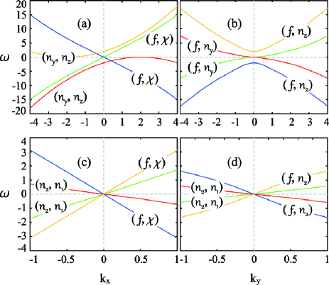
Figure 1: (color online) Excitation modes of plane-wave (upper panels) and stripe (lower panels) state along the $k_{x}$ (left column, $k_{y}=0$) and $k_{y}$ (right column, $k_{x}=0$) directions. Rashba strength $\kappa=1$ sets the unit for the $x$-axis and $g_{c}=10$. Only the four gapless branches are shown in the lower panels for the stripe state. We choose $g_{s}=0$ for all cases. Shown inside the parentheses are the two components contributing the most and the second most to each eigenvector.

The stripe solution yields $\rho_{0}=1$, ${\bf v}_{0}=0$, and ${\bf n}_{0}=(0,-\sin\theta,\cos\theta)$, where $\theta=2\kappa x$. The spin order is a spiral with the plane of spin rotation orthogonal to the propagation vector ${\bf q}=2\kappa{\bf e}_{x}$. Only the fluctuations of ${\bf n}$ need to be parameterized differently from the plane-wave case, as ${\bf n}={\bf n}_{0}+\eta_{1}{\bf e}_{1}+\eta_{2}{\bf e}_{2}$, where ${\bf e}_{1}=(1,0,0)$, ${\bf e}_{2}=(0,\cos\theta,\sin\theta)$, and ${\bf n}_{0}$ form the three orthogonal axes in the rotating Frenet-Serret frame lamacraft . Contrary to the plane-wave case, we have a nonzero effective electric field contribution to the Euler equation as $e_{x}=-\kappa\dot{\eta}_{1}$ and correspondingly, the Mermin-Ho constraint in the case of stripe state is solved by $\nu_{x}+\kappa\eta_{1}=\partial_{x}f,\nu_{y}=\partial_{y}f$. Inserting them back into the hydrodynamic equations yields

$$-\omega\chi+\frac{i}{2}\kappa k_{y}\chi^{-}+i{\bf k}^{2}f+\frac{\kappa}{2}k_{y}\eta^{+}_{2} = 0,$$

$$(\frac{i}{4}{\bf k}^{2}-ig_{c})\chi-\omega f+\frac{i}{2}\kappa k_{y}f^{-}-\frac{\kappa}{4}k_{y}\eta^{+}_{1} = 0,$$

$$-\kappa k_{y}f^{+}-\omega\eta_{1}-\frac{i}{2}\kappa k_{y}\eta^{-}_{1}+\frac{i}{2}{\bf k}^{2}\eta_{2} = 0,$$

$$\frac{\kappa}{2}k_{y}\chi^{+}-\frac{i}{2}{\bf k}^{2}\eta_{1}-2i\kappa^{2}\eta_{1}-\omega\eta_{2}+\kappa k_{x}\eta_{2}-\frac{i}{2}\kappa k_{y}\eta^{-}_{2} = 0,$$

where $m^{\pm}=m({\bf k}-{\bf q})\pm m({\bf k}+{\bf q})$ ($m=\chi,f,\eta_{1},\eta_{2}$) and un-superscripted variables are at momentum ${\bf k}$. Coupling of the ${\bf k}$-modes displaced by $\pm{\bf q}$ is a consequence of the ground state being a modulated state, thus no way to write the excitation equations into the $4\times 4$ matrix form as in the plane wave case. Numerical diagonalization yields the spectrum shown in Fig. 1(c) and 1(d). Analogous “helimagnon band” was identified in a spiral magnet MnSi rosch . For the parameters we choose, four linear sound modes with mode contributions as labeled in Fig. 1(c) and 1(d) exist near $k_{x}=k_{y}=0$, which is different from the plane-wave case. Bogoliubov analysis of the GP equation yields identical spectra for the stripe state as well.

In summary, we have derived the mathematical mapping of the Rashba spin-orbit-coupled BEC Hamiltonian in terms of hydrodynamic variables. The mapping highlights the connection of the present system to the chiral magnets. The hydrodynamic equation for mass conservation, as well as Euler and Landau-Lifshitz equations for superfluid velocity and spin dynamics, respectively, are derived. The mass current contains an extra magnetization term due to the Rashba coupling. As applications of hydrodynamic approach, we studied the elementary excitation modes of the plane-wave and stripe states of Rashba-BEC, featuring the different behaviors of fluctuations around the two degenerate ground states and the coupled behavior of spin and superflow velocity in the presence of Rashba coupling.

H. J. H. is supported by NRF grant (No. 2011-0015631). Useful discussion with Hui Zhai at the early stage of research is gratefully acknowledged.

References

- (1) Y.-J. Lin, K. Jiménez-Garcia, and I. B. Spielman, Nature 471, 83 (2011).
- (2) J. Dalibard, F. Gerbier, G. Juzeliunas, and Patrik Öhberg, Rev. Mod. Phys. 83, 1523 (2011).
- (3) C. Wang, C. Gao, C.-M. Jian, and H. Zhai, Phys. Rev. Lett. 105, 160403 (2010).
- (4) S.-K. Yip, Phys. Rev. A 83, 043616 (2011); Z. F. Xu, R. Lu, and L. You, Phys. Rev. A 83, 053602 (2011); T. Kawakami, T. Mizushima, and K. Machida, Phys. Rev. A 84, 011607 (2011); C. Wu, I. Mondragon-Shem, and X.-F. Zhou, Chin. Phys. Lett. 28, 097102 (2011); T.-L. Ho and S. Zhang, Phys. Rev. Lett. 107, 150403 (2011); Y. Zhang, L. Mao, and C. Zhang, Phys. Rev. Lett. 108, 035302 (2012).
- (5) Y. A. Bychkov and E. I. Rashba, JETP Lett. 39, 78 (1984).
- (6) S. Sinha, R. Nath, and L. Santos, Phys. Rev. Lett. 107, 270401 (2011); H. Hu, B. Ramachandhran, H. Pu, and X.-J. Liu, Phys. Rev. Lett. 108, 010402 (2012).
- (7) X.-Q. Xu and J. H. Han, Phys. Rev. Lett. 107, 200401 (2011); J. Radić, T. A. Sedrakyan, I. B. Spielman, and V. Galitski, Phys. Rev. A 84, 063604 (2011); X.-F. Zhou, J. Zhou, and C. Wu, Phys. Rev. A 84, 063624 (2011).
- (8) M. Burrello and A. Trombettoni, Phys. Rev. Lett. 105, 125304 (2010); Phys. Rev. A 84, 043625 (2011).
- (9) C.-M. Jian and H. Zhai, Phys. Rev. B 84, 060508 (2011).
- (10) Q. Zhu, C. Zhang, and B. Wu, arXiv:1109.5811 (2011).
- (11) R. Barnett, S. Powell, T. Graß, M. Lewenstein, and S. Das Sarma, Phys. Rev. A 85, 023615 (2012).
- (12) I. M. Khalatnikov, An Introduction to the Theory of Superfluidity, translated by P. C. Hohenberg (W. A. Benjamin Inc., New York, 1965).
- (13) A. Lamacraft, Phys. Rev. A 77, 063622 (2008).
- (14) R. Barnett, D. Podolsky, and G. Refael, Phys. Rev. B 80, 024420 (2009).
- (15) R. W. Cherng, V. Gritsev, D. M. Stamper-Kurn, and E. Demler, Phys. Rev. Lett. 100, 180404 (2008).
- (16) D.-H. Lee and C. L. Kane, Phys. Rev. Lett. 64, 1313 (1990).
- (17) J. H. Han, J. Zang, Z. Yang, J.-H. Park, and N. Nagaosa, Phys. Rev. B 82, 094429 (2010).
- (18) T.-L. Ho, Phys. Rev. Lett. 81, 742 (1998); T. Ohmi and K. Machida, J. Phys. Soc. Jpn., 67, 1822 (1998).
- (19) V. Ambegaokar, P. G. deGennes, and D. Rainer, Phys. Rev. A 9, 2676 (1974).
- (20) H. Katsura, N. Nagaosa, and A. V. Balatsky, Phys. Rev. Lett. 95, 057205 (2005); M. Mostovoy, Phys. Rev. Lett. 96, 067601 (2006).
- (21) N. D. Mermin and T.-L. Ho, Phys. Rev. Lett. 36, 594 (1976).
- (22) M. Janoschek, F. Bernlochner, S. Dunsiger, C. Pfleiderer, P. Böni, B. Roessli, P. Link, and A. Rosch, Phys. Rev. B 81, 214436 (2010).