Gaussian Matrix Product States

Abstract
We introduce Gaussian Matrix Product States (GMPS), a generalization of Matrix Product States (MPS) to lattices of harmonic oscillators. Our definition resembles the interpretation of MPS in terms of projected maximally entangled pairs, starting from which we derive several properties of GMPS, often in close analogy to the finite dimensional case: We show how to approximate arbitrary Gaussian states by MPS, we discuss how the entanglement in the bonds can be bounded, we demonstrate how the correlation functions can be computed from the GMPS representation, and that they decay exponentially in one dimension, and finally relate GMPS and ground states of local Hamiltonians. [This work originally appeared as Sec. VII of quant-ph/0509166, and is published in the Proceedings on the conference on Quantum information and many body quantum systems, edited by M. Ericsson and S. Montangero, pg. 129 (Edizioni della Normale, Pisa, 2008).]

1 Introduction

In the last years, there has been considerable activity on the border between quantum information theory and condensed matter physics, and quantum information concepts have successfully been applied to the description of quantum many-body systems. An important step has been the interpretation of Matrix Product States (MPS) in terms of projected maximally entangled pairs. MPS form a hierarchy of states which prove very successful as a variational ansatz for simulating ground states of one-dimensional quantum systems, as done in the Density Matrix Renormalization Group (DMRG) method [1, 2]. From the perspective of quantum information, MPS are formed by taking virtual maximally entangled pairs between adjacent sites and applying a linear map on each site to obtain the physical system [3]. This entanglement-based description led to a better understanding of MPS and gave rise to new algorithms and extensions of DMRG to e.g. thermal states, time evolutions, and higher dimensional systems [4, 5, 6, 7], but also to new analytical tools for investigating e.g. quantum phase transitions, renormalization group transformations, or the sequential generation of quantum states [8, 9, 10].

Given the success of the MPS framework in the description of finite-dimensional spin systems, it is natural to look for generalizations to e.g. bosonic or fermionic systems. In this paper, we introduce bosonic Gaussian Matrix Product States (GMPS), which describe Gaussian states on lattices of harmonic oscillators (i.e., bosonic modes). Such systems are frequently realized in physical setups, e.g. by the vibrational modes of ions in linear traps or by arrays of nanomechanical oscillators, and since they are typically goverened by quadratic Hamiltonians, their ground and thermal states are Gaussian.

Our definition of GMPS resembles the quantum information perspective on MPS, where one takes maximally entangled pairs and applies a linear map to obtain the physical system. Starting from this definition, we show that every (translation invariant) Gaussian state can be represented as a (translation invariant) GMPS, and discuss how to minimize the amount of entanglement used in the bonds – different from the finite-dimensional case, this is an issue since bosonic bonds can carry an unbonded amount of entanglement. We discuss the properties of two-point correlation functions of GMPS and show that they can be easily computed from the GMPS representation; for the case of pure one-dimensional GMPS, we prove that the correlations decay exponentially (as it is the case in finite dimensions) and explicitly derive the correlation length. We end our discussion on GMPS by showing that – again in analogy to the finite dimensional case – every GMPS is the ground state of a local Hamiltonian.

Since Gaussian states are completely characerized by their second moments and thus by a number of parameters quadratic in the system size, unlike for spin systems Gaussian MPS will not by themselves yield an exponentially more efficient parametrization. However, they can be used to describe translational invariant states with a constant number of parameters and thus also in the limit of an infinite chain. Moreover, the GMPS parametrization should have favorable properties e.g. for variational minimizations with respect to local observables.

The results presented in this work have already been applied in [11, 12].

2 Gaussian states

Consider a system of $N$ bosonic modes which are characterized by $N$ pairs of canonical operators $(Q_{1},P_{1},\ldots,Q_{N},P_{N})=:R$, and where the canonical commutation relations (CCR) are governed by the symplectic matrix $\sigma$ via

$$\big{[}R_{k},R_{l}\big{]}=i\sigma_{kl}\;,\quad\sigma=\bigoplus_{n=1}^{N}\left(\begin{array}[]{cc}0&1\\ -1&0\end{array}\right)\;.$$

Then, Gaussian states are defined as states which have a Gaussian Wigner distribution in phase space. Those state are frequently met in physics, since ground or thermal states of quadratic Hamiltonians are Gaussian states, and evolution under a quadratic Hamiltonian leaves Gaussian states Gaussian. They are completely characterized by their first moments $d_{k}=\mathrm{tr}{\big{[}\rho R_{k}\big{]}}$ (which can be changed by local operations, so that we set them to zero w.l.o.g.) and their covariance matrix (CM)

$$\gamma_{kl}=\mathrm{tr}\Big{[}\rho\big{\{}R_{k}-d_{k},R_{l}-d_{l}\big{\}}_{+}\Big{]}\;,$$ (1)

where $\{\cdot,\cdot\}_{+}$ is the anticommutator. The CM satisfies $\gamma\geq i\sigma$, which expresses Heisenberg’s uncertainty relation and is equivalent to the positivity of the corresponding density operator $\rho\geq 0$. Purity of the state is characterized by $\det\gamma=1$ or equivalently $(\sigma\gamma)^{2}=-1\!\!1$.

When the state under consideration is translational invariant, it often proves convenient to describe it in the Fourier basis. For simplicity, let us consider a one-dimensional translational invariant chain of length $N$ with periodic boundaries and reorder the canonical operators such that $R=(Q_{1},\ldots,Q_{N},P_{1},\ldots,P_{N})$. Then,

$$\gamma=\left(\begin{array}[]{cc}\gamma_{Q}&\gamma_{QP}\\ \gamma_{QP}^{T}&\gamma_{P}\end{array}\right)\ ,$$

and translational invariance is reflected by the fact that any matrix element $A_{kl}$ (where $A\in\{\gamma_{Q},\gamma_{P},\gamma_{QP}\}$) depends only on the distance $k-l$ (which is understood $\mathrm{mod}\ N$), so we can write $A_{k-l}:=A_{kl}$. Matrices of this type are called circulant and are simultaneously diagonalized by the Fourier transform. We write the diagonal elements of the Fourier transform as a function of the angle $\phi=2\pi m/N$ for $m=0,\dots,N-1$; the Fourier transform of a cirulant matrix $A$ then reads $\hat{A}(\phi)=\sum A_{n}e^{-in\phi}$.

An interesting property of translational invariant pure states with one mode per site is that they are point symmetric [13]. This can readily be seen from the representation

$$\gamma=\left(\begin{array}[]{cc}\gamma_{Q}&\gamma_{QP}\\ \gamma_{QP}^{T}&\gamma_{P}\end{array}\right)=\left(\begin{array}[]{cc}X&XY\\ YX&\ X^{-1}+YXY\end{array}\right)$$

in $Q$-$P$ partitioning with $X>0$, $Y=Y^{T}$ real [14], since $X$ and $Y$ have to be circulant and therefore commute. Hence, $\gamma_{QP}=XY=YX=\gamma_{QP}^{T}$, i.e., $\gamma$ is point symmetric. Note that this implies in particular that the Fourier transform $\hat{\gamma}(\phi)$ is real.

3 Gaussian Matrix Product States

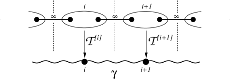
Figure 1: Construction of Gaussian Matrix Product States (GMPS). GMPS are obtained by taking a fixed number $M$ of maximally entangled (i.e., EPR) pairs shared by adjacent sites, and applying an arbitrary $2M$ to $1$ mode Gaussian operation $\mathcal{T}^{[i]}$ on site $i$.

In the following, we introduce Gaussian matrix product states (GMPS). The definition resembles the physical interpretation of finite-dimensional matrix product states as projected entangled pairs: In finite dimensions, MPS can be described by taking maximally entangled pairs of dimension $D$ between adjacent sites and applying arbitrary local operations on each site, thus mapping the $D\times D$ dimensional input (the virtual system) to a $d$-dimensional output state (the physical system). Similarly, GMPS are obtained by taking a number of entangled bonds and applying local (not necessarily trace-preserving) operations $\mathcal{T}^{[i]}$, where the boundary conditions can be taken either open or closed. Any GMPS is completely described by the type of the bonds and by the operations $\mathcal{T}^{[i]}$. Note that this construction holds independent of the spatial dimension. For one dimension, it is illustrated in Fig. 1. As matrix product states are frequently used to describe translationally invariant systems, an inportant case is given if all maps are identical, $\mathcal{T}^{[i]}=\mathcal{T}\ \forall i$.

In order to define MPS in the Gaussian world, we have to decide on the type of the bonds as well as on the type of operations. We choose both the bonds to be Gaussian states and the operations to be Gaussian operations, i.e., operations mapping Gaussian inputs to Gaussian outputs. For now, we will take the bonds to be maximally entangled (i.e., EPR) states, such that the only parameter originating from the bonds is the number $M$ of EPRs. We show later on how the case of finitely entangled bonds can be easily embedded.

As to the operations, we will allow for arbitrary Gaussian operations. Operations of this type are most easily described by the Jamiolkowski isomorphism [15]. There, any Gaussian operation $\mathcal{T}$ which maps $N$ input modes to $M$ output modes can be described by an $N+M$ mode covariance matrix $\Gamma$ with block $B$ (input) and $C$ (output). The corresponding map on some input state $\gamma_{\mathrm{in}}$ in mode $A$ is implemented by projecting the modes $A$ and $B$ onto an EPR state as shown in Fig. 2, such that the output state $\mathcal{T}(\gamma_{\mathrm{in}})$ is obtained in mode $C$. Conversely, the matrix $\Gamma$ which represents the channel $\mathcal{T}$ is obtained by applying the channel to one half of a maximally entangled state. The duality between $\mathcal{T}$ and $\Gamma$ is most easily understood in terms of teleportation, and shows that this characterization encompasses all Gaussian operations. Note that the protocol of Fig. 2 can be always made trace-preserving by projecting onto the set of phase-space displaced EPR states and correcting the displacement of mode $C$ according to the measurement outcome [16].

In the following, we will denote all maps $\mathcal{T}$ by their corresponding CM $\Gamma$. Sometimes, we will speak of the modes $B$ and $C$ as input and output ports of $\Gamma$, respectively.

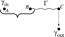
Figure 2: The Jamiolkowski isomorphism. The Gaussian channel described by the state $\Gamma$ can be implemented by projecting the input state $\gamma_{\mathrm{in}}$ (mode $A$) and the input port of $\Gamma$ (mode $B$) onto the EPR state (symbolized by curly brackets). In case of success, the output is obtained in mode $C$. The operation can be made trace-preserving by measuring in a basis of displaced EPR states, and displacing $C$ according to the measurement outcome.

We now discuss how the covariance matrix of the output will depend on the CM of the input and on the channel $\Gamma$ [16, 17]. This is most easily computed in the framework of characteristic functions [18]. The characteristic function of the output is given by

$$\chi_{C}(\xi_{C})\propto\int e^{-\xi_{A}^{T}\gamma_{\mathrm{in}}\xi_{A}}e^{-\xi_{BC}^{T}\Gamma\xi_{BC}}\delta(x_{A}-x_{B})\delta(p_{A}+p_{B})\mathrm{d}\xi_{AB}\ ,$$

and by integrating over subsystem $A$, we obtain

$$\chi_{C}(\xi_{C})\propto\int e^{-\xi_{BC}^{T}M\xi_{BC}}\mathrm{d}\xi_{B}$$

with

$$M=\left(\begin{array}[]{cc}\theta\gamma\theta+\Gamma_{B}&\Gamma_{BC}\\ \Gamma_{CB}&\Gamma_{C}\end{array}\right)\ .$$

Basically, the integration $\int{\mathrm{d}}\xi_{A}\delta(x_{A}-x_{B})\delta(p_{A}+p_{B})$ does the following: first, it applies the partial transposition $\theta\equiv\left(\begin{smallmatrix}1&0\\ 0&-1\end{smallmatrix}\right)$ to one of the subsystems, and second, it collapses the two systems $A$ and $B$ in the covariance matrix by adding the corresponding entries. The integration over $\xi_{B}$, on the other hand, leads to a state whose CM is the Schur complement of $M_{11}$, $M_{22}-M_{21}M_{11}^{-1}M_{12}$, such that the output state is described by the CM

$$\gamma_{\mathrm{out}}=\Gamma_{C}-\Gamma_{CB}\frac{1}{\Gamma_{B}+\theta\gamma_{\mathrm{in}}\theta}\Gamma_{BC}\ .$$

Let us briefly summarize how to perform projective measurements onto the EPR state in the framework of CMs, where we denote the measured modes by $A$ and $B$, while $C$ is the remaining part of the system. First, apply the partial transposition to $B$, second, collapse $A$ and $B$, and third, take the Schur complement of the collapsed mode $AB$, which gives the output CM of $C$.

In analogy to the finite-dimensional case, we will focus on pure GMPS. Particularly, a GMPS is pure if the $\Gamma^{[i]}$ which describe the operations $\mathcal{T}^{[i]}$ are taken to be pure, which we assume from now on. Let us finally emphasize that the given defintion of MPS holds independent of the spatial dimension of the system, as do most of the following results, and in fact applies to an arbitrary graph.

4 Completeness of Gaussian MPS

In the following, we show that any pure and translational invariant state can be approximated arbitrarily well by translational invariant Gaussian matrix product states, i.e., GMPS with identical local operations $\mathcal{T}$. (Without translational invariance, this is clear anyway: the complete state is prepared locally and teleported to its destination using the bonds.) The proof is presented for one dimension, but can be extended to higher spatial dimensions. Note that a similar result also holds for finite-dimensional MPS [19].

Given a translational invariant state $\gamma$, there is a translational invariant Hamiltonian $H$ which transforms the separable state $1\!\!1$ into $\gamma$, $\gamma=SS^{T}$, $S=e^{\sigma H}$. It has been shown [20] that this time evolution can be approximated arbitrarily well by a sequence of translational invariant local (one-mode) and nearest neighbor (two-mode) Hamiltonians $H_{j}$,

$$e^{\sigma H}\approx\prod_{j=1}^{J}e^{\bigoplus_{n}\sigma H_{j}}\ ,$$ (2)

where the $H_{j}$ act on one or two modes, respectively, and approach the identity for growing $J$.

Clearly, translational invariant local Hamiltionians can be implemented by local maps without using any EPR bonds. In the following, we show how translational invariant nearest-neighbor interactions can be implemented by exploiting the entanglement of the bonds. The whole procedure is illustrated in Fig. 3 and requires two EPR pairs per site. We start with some initial state $\gamma_{\mathrm{in}}$ onto which we want to apply $S_{\oplus}=e^{\bigoplus\sigma H_{j}}\approx 1\!\!1+\bigoplus_{n}\sigma H_{j}$.

First, we perform local EPR measurements between the modes of $\gamma_{\mathrm{in}}$ and one of the bonds in order to teleport the modes of $\gamma_{\mathrm{in}}$ to the left, cf. Fig. 3a. Then, the infinitesimal symplectic operation $S=e^{\sigma H_{j}}$ is applied to the left-teleported mode and the second bond, Fig. 3b. In the last step, another EPR measurement is performed which teleports the left-teleported mode back to the right, and “into” the mode on which the adjacent $S$ was applied. As the operations $e^{\sigma H_{j}}\approx 1\!\!1+\sigma H_{j}$ all commute, the “nested” application of the nearest neighbor symplectic operations $S$ indeed give $S_{\oplus}$, and thus the remaining mode really contains the output $\gamma_{\mathrm{out}}=S_{\oplus}\gamma_{\mathrm{in}}S_{\oplus}^{T}$. The whole decomposition (2) can be implemented by iterated application of the whole protocol of Fig. 3.

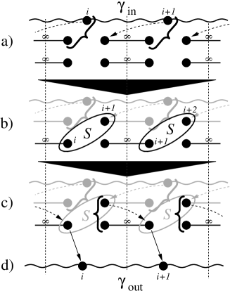
Figure 3: Implementation of a translational invariant nearest neighbor Hamiltonian in a translational invariant fashion. Starting from $\gamma_{\mathrm{in}}$, the input is first teleported to the left, then, the infinitesimal time evolution $S=e^{\sigma H}$, $H\ll 1$, is performed, and finally, the state is teleported back.

5 GMPS with finitely entangled bonds

Let us now consider the entanglement contained in the bonds and show that infinitely entangled bonds can be replaced by finitely entangled ones. Intuitively, this should be possible whenever the channel $\mathcal{T}^{[i]}$ destroys some of the entanglement of the bond anyway, i.e., $\Gamma^{[i]}$ is non-maximally entangled. In that case, it should be possible to use a less entangled bond while choosing a channel which does not destroy entanglement any more.

The method is illustrated in Fig. 4. Again, for reasons of clarity we restrict to one dimension and one bond. The argument however applies independent of the spatial dimension and the number of bonds. The only restriction we have to make is the restriction to pure GMPS, i.e., those with pure $\Gamma^{[i]}$.

Consider a GMPS with local channels given by $\Gamma^{[i]}$ and infinitely entangled bonds, Fig. 4a. First, apply a Schmidt decomposition [21] to $\Gamma^{[i]}$ in the partition $A|BC$, which can be always done as long as $\Gamma^{[i]}$ is pure. The Schmidt decomposition allows us to rewrite the state as shown in Fig. 4b – an entangled state between modes $A$ and $C$ with two-mode squeezing $r^{[i]}$, $B$ in the coherent state $1\!\!1$, and sympectic operations $S_{A}^{[i]}$ and $S_{BC}^{[i]}$ which are applied to modes $A$ and $BC$, respectively. As the bond itself is infinitely entangled, we can teleport the sympectic operation through the bond to the next site as indicated in Fig. 4b. Then, $S_{A}^{[i+1]}$ can be merged with $S_{BC}^{[i]}$ to a new operation $\tilde{S}^{[i]}$ acting on modes $B$ and $C$ of site $i$ (Fig. 4c). Finally, in the triples consisting of one maximally entangled state, one non-maximally entangled state, and the projection onto the EPR state, the maximally and the non-maximally entangled state can be swapped, resulting in Fig. 4d. There, we have finitely entangled bonds, while the infinite entanglement has been moved into the new maps $\tilde{\Gamma}^{[i]}$.

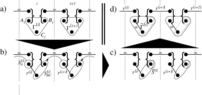
Figure 4: How to make the bonds of GMPS finitely entangled. a) The initial MPS. b) Do a Schmidt decomposition of the original map $\Gamma$. c) Move the $S^{[i]}_{A}$ through the infinitely entangled bond to the next site. d) Swap the finitely and the infinitely entangled pair.

It is tempting to apply this construction to the completeness proof of the preceding section in order to obtain a construction which is less wasting with respect to resources. However, for any iterative protocol this is most likely difficult to achieve. The reason for this is found in the no-distillation theorem which states that with Gaussian operations, it is not possible to increase the amount of entanglement between two parties [16]. Particularly, this implies that in each step of an iterative protocol, the bonds need to have at least as much entanglement as can be obtained at the output of this step, maximized over all inputs where the entanglement is increased. This is indeed a severe restriction, although it does not imply the impossibility of such a protocol. One could, e.g., create a highly entangled state in the first step and then approach the desired state by decreasing the entanglement in each step. Still, it seems most likely that a sequence of MPS which approach a given state efficiently will have to involve more and more bonds simultaneously and thus cannot be constructed in an iterative manner.

6 Correlation functions of Gaussian MPS

In this section, we show how to compute correlation functions from the maps $\Gamma^{[i]}$ which describe the GMPS. We show that this can be done efficiently, i.e., in a time which is polynomial in the systems size, independent of the dimension of the graph. This is different from the finite dimensional case, where correlation functions of e.g. two-dimensional MPS cannot be computed efficiently [22]. Of course, this is not too surprising given that Gaussian states can be fully characterized by a number of paramaters quadratic in the number of modes.

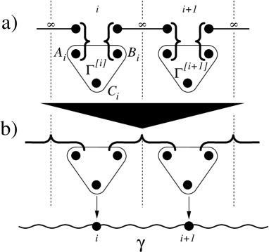
Figure 5: If the local operations are described by states $\Gamma^{[i]}$ via the Jamiolkowski isomorphism, the construction of GMPS can be simplified by replacing the measurement-bond-measurement triples by a simple projection onto the EPR state.

Let us start with the general case of different $\Gamma^{[i]}$, as in Fig. 5a. The calculation can be facilitated by the simple observation that the triples consisting of two projective measurements and one EPR pair can be replaced by a single projection onto the EPR state, Fig. 5b. It follows that we can apply the formalism for projective measurements onto the EPR state which we presented in Section 3. Starting from $\bigoplus_{i}\Gamma^{[i]}$, we first partially transpose all $B$ modes, then collapse $A_{i+1}$ and $B_{i}$ for all $i$, and finally take the Schur complement of the merged mode. In case of periodic boundary conditions, this can be expressed by the transformation matrix

$$\Pi=\left(\begin{array}[]{ccc}1\!\!1_{A}&\mathcal{R}\theta_{B}&0\\ 0&0&1\!\!1_{C}\end{array}\right)$$ (3)

which maps $ABC$ onto $A^{\prime}C$, where $\theta_{B}\equiv\theta\otimes 1\!\!1$ is the partial transposition on system $B$, and $\mathcal{R}$ is the circulant right shift operator, $(\mathcal{R})_{ij}=\delta_{i,j+1\mod N}\otimes 1\!\!1$. Then, the output state, i.e., the GMPS characterized by $\Gamma^{[i]}$, is

$$\gamma=\mathrm{SC}_{A^{\prime}}\left[\Pi\left(\bigoplus_{i}\Gamma^{[i]}\right)\Pi^{T}\right]\ ,$$

where $\mathrm{SC}_{X}(U)$ is the Schur complement of the $X$ part of $U$, $\mathrm{SC}_{X}(U)=U_{YY}-U_{YX}U_{XX}^{-1}U_{XY}$. For open boundary conditions, the matrix $\Pi$ has to be modified accordingly at the boundaries. All the involved operations scale polynomially in the product $NM$ of the number of sites $N$ and the number of modes $M$.

In case all the local maps are chosen equal, $\Gamma^{[i]}\equiv\Gamma\ \forall i$, the above formula can be simplified considerably. Therefore, note that the Fourier transform can be taken into the Schur complement, and that $\Pi$ as well as $\bigoplus_{i=1}^{N}\Gamma^{[i]}=\Gamma\otimes 1\!\!1_{N}$ are blockwise circulant so that both are diagonalized by the Fourier transform. Thereby, $\Gamma\otimes 1\!\!1$ is mapped onto the constant function $\Gamma$, and the same holds for $1\!\!1$ and $\theta$ in (3). The right shift operator $\mathcal{R}$, on the other hand, is transformed to $e^{i\phi}$1​​1: the EPR measurement performed between adjacent sites leads to a complex phase of $\phi$. Altogether, we have

$$\hat{\Pi}=\left(\begin{array}[]{ccc}1\!\!1_{A}&e^{i\phi}\theta_{B}&0\\ 0&0&1\!\!1_{C}\end{array}\right)\ ;\quad\hat{\gamma}=\mathrm{SC}_{A^{\prime}}\left[\hat{\Pi}\,\Gamma\,\hat{\Pi}^{\dagger}\right]\ .$$

Directly expressed in terms of the map $\Gamma$, this reads

$$\hat{\gamma}(\phi)=\Gamma_{C}-\Gamma_{C|AB}\,\hat{\Lambda}\frac{1}{\hat{\Lambda}\,\Gamma_{AB|AB}\,\hat{\Lambda}^{\dagger}}\,\hat{\Lambda}^{\dagger}\,\Gamma_{AB|C}$$ (4)

where $\hat{\Lambda}=(1\!\!1_{A}\,;\,e^{i\phi}\theta_{B})$ is the upper left subblock of $\hat{\Pi}$.

7 States with rational trigonometric functions as Fourier transforms

Let us now restrict to pure MPS (i.e., those for which $\Gamma$ is pure) with one mode per site. As we have shown in Section 2, those states have reflection symmetry and therefore $\hat{\gamma}(\phi)=\gamma_{0}+2\sum_{n\geq 0}\gamma_{n}\cos(n\phi)$ is real. This implies that the sines in (4) can only appear in even powers $\sin^{2n}\phi=(1-\cos^{2}\phi)^{n}$. Therefore, the Fourier transform $\hat{\gamma}$ of any pure Gaussian MPS, which is a $2\times 2$ matrix valued function of $\phi$, has elements which are rational functons of $\cos(\phi)$, $(\hat{\gamma}(\phi))_{xy}=p_{xy}(\cos(\phi))/q_{xy}(\cos(\phi))$ with $p$, $q$ polynomials. The degree of the polynomials is limited by the size of $\hat{\Lambda}\Gamma_{AB}\hat{\Lambda}^{\dagger}$, and thus by the number $M$ of the bonds. One can easily check that $\dim p\leq 2M+1$ and $\dim q\leq 2M$.

For the following discussion, let us write those rational functions with a common denominator $d$,

$$\hat{\gamma}(\phi)=\frac{1}{d(\cos(\phi))}\left(\begin{array}[]{cc}q(\cos(\phi))&r(\cos(\phi))\\ r(\cos(\phi))&p(\cos(\phi))\end{array}\right)\ ,$$ (5)

where $q$, $p$, $r$, and $d$ are polynomials of degree $L$. Then, the set of all such $\hat{\gamma}$ with $L\geq 2M+1$ encompasses the set of translational invariant GMPS with $M$ bonds. Computing correlation functions in a lattice of size $N$ can be done straightforwardly in this representation by taking the discrete Fourier transform of $\hat{\gamma}(\phi)$ which scales polynomially with $N$, and in the following section we show that for one dimension, the correlations can be even computed exactly in the limit of an infinite chain.

It is interesting to note that $\gamma(\phi)$ is already determined up to a finite number of possibilities by fixing $r$ and $d$. Since $\gamma$ is pure, $1=\det\gamma=\det\hat{\gamma}$, and therefore, $pq=d^{2}+r^{2}$. Therefore, the zeros of $pq$ are the zeros of $d^{2}+r^{2}$, such that the only freedom is to choose how to distribute the zeros on $p$ and $q$. On the contrary, fixing only $q$ and $d$ does not give sufficient information, while choosing $p$, $q$ and $d$ (i.e., the diagonal of $\hat{\gamma}$) does not ensure that there exists a polynomial $r$ such that $pq-r^{2}=d^{2}$.

From the above, it follows that $2L+1$ parameters are sufficient to describe $\hat{\gamma}(\phi)$, where $L$ is still the degree of the polynomials. This encloses all translational invariant Gaussian MPS with bond number $M\leq(L-1)/2$, which need $(2M+1)(2M+2)=L(L+1)$ parameters. Therefore, the class of states where $\hat{\gamma}(\phi)$ is a rational function of $\cos(\phi)$ is a more efficient description of translationally invariant states than Gaussian MPS are.

Let us stress once more that the results of this section hold for arbitrary spatial dimension.

8 Correlation length

In the following, we show that the correlations of one-dimensional GMPS decay exponentially, and we explicitly derive the correlation length. The derivation only makes use of the representation (5) of Gaussian MPS and thus holds for the whole class of states where the Fourier transform is a rational function of the cosine. We will restrict to the case where the state $\Gamma$ associated to the GMPS map has no diverging entries, which corresponds to the case where the denominator $d(\cos(\phi))$ in (5) has no zero on the unit circle.

The correlations are directly obtained by back-transforming the elements of $\hat{\gamma}(\phi)$, which are rational functions $[\hat{\gamma}(\phi)]_{s}=s(\cos(\phi))/d(\cos(\phi))$, $s\in\{p,q,r\}$; in the limit of an infinite chain,

$$(\gamma_{s})_{n}=\frac{1}{2\pi}\int_{0}^{2\pi}\frac{s(\cos(\phi))}{d(\cos(\phi))}e^{in\phi}{\mathrm{d}}\phi\ .$$

Now transform $s$, $d$ to complex polynomials via $\cos(\phi)\rightarrow(z+1/z)/2$, and expand with $z^{K}$, $\tilde{s}(z):=z^{K}s(z)$, $\tilde{d}(z):=z^{K}d(z)$, where $K$ is chosen large enough to make $\tilde{s}$, $\tilde{d}$ polynomials in $z$. Then,

$$(\gamma_{s})_{n} = \frac{1}{2\pi i}\int_{\mathcal{S}^{1}}\frac{\tilde{s}(z)z^{n-1}}{\tilde{d}(z)}{\mathrm{d}}z$$

$$= \sum_{z_{i}:\tilde{d}(z_{i})=0}\frac{1}{(\nu_{i}-1)!}\underbrace{\left.\frac{{\mathrm{d}}^{\nu_{i}-1}}{{\mathrm{d}}z^{\nu_{i}-1}}\left[\frac{\tilde{s}(z)z^{n-1}}{\tilde{d}_{i}(z)}\right]\right|_{z=z_{i}}}_{D_{i}}$$

by the calculus of residues, where $\nu_{i}$ is the order of the zero $z_{i}$ in $\tilde{d}$ and $\tilde{d}_{i}(z)(z-z_{i})^{\nu_{i}}=\tilde{d}(z)$. For $n>\nu_{i}$, $D_{i}\propto z_{i}^{(n-\nu_{i})}$, and it follows that the correlations decay exponentially, where the correlation length is given by the largest zero of $q(z)$ inside the unit circle.

This proof only holds for one-dimensional GMPS. However, it can be proven for arbitrary spatial dimensions that the correlations decay faster than any polynomial by iterated integration by parts with respect to one component of $\phi$, cf. [13].

9 Gaussian MPS as ground states of local Hamiltonians

Finally, let us focus on the relation of translational invariant Gaussian MPS and local Hamiltonians. We prove that every GMPS is the ground state of a local Hamiltonian, while conversely most Hamiltonians do not have GMPS as an exact ground state – again, this is in close analogy to the finite-dimensional case [19]. Once more, the proof only requires the state to be of the form Eq. (5). We will make use of some results on ground states of translational invariant quadratic Hamiltonians presented in [13]. Define the Hamiltonian matrix $H\geq 0$ via the Hamilton operator $\mathcal{H}$ by virtue of $\mathcal{H}=\sum H_{kl}R_{k}R_{l}$, as well as the spectral function $\mathcal{E}=\sqrt{\mathrm{det}\,\hat{H}}$. Then, the ground state is given by

$$\hat{\gamma}=(\mathcal{E}\oplus\mathcal{E})^{-1}\sigma\hat{H}\sigma^{T}$$ (6)

and has energy $\tfrac{1}{2}\mathrm{tr}\,\mathcal{E}$.

Given a pure state $\gamma$ with Fourier transform (5), define

$$\hat{H}(\phi)=\left(\begin{array}[]{cc}p(\cos(\phi))&-r(\cos(\phi))\\ -r(\cos(\phi))&q(\cos(\phi))\end{array}\right)$$ (7)

Then, $H$ corresponds to a local Hamiltonian – the interaction range is the degree of $p,q,r$ – and $\mathcal{E}(\phi)=\big{[}\sqrt{pq-r^{2}}\;\big{]}(\cos\phi)=d(\cos\phi)$, which together with (6) proves that $\gamma$ is the ground state of $H$.

Let us also have a brief look at the converse question: Given a local Hamiltonian, when will it have a GMPS as its ground state? Any local and translational invariant Hamiltonian has a Fourier transform which consists of polynomials in $\cos(\phi)$, and thus we adapt the notation of Eq. (7). Then, following Eq. (6) the ground state is represented by a rational function of $\cos(\phi)$ in Fourier space exactly if $pq-r^{2}=d^{2}$ is the square of another polynomial. In terms of the original Hamiltonian, this implies that $H_{Q}H_{P}-H_{QP}^{2}$ has to be the square of another banded matrix. For example, for $H=V\oplus 1\!\!1$ one would need $V=X^{2}$ with $X$ again a banded matrix [23].

References

- [1] S. R. White, Phys. Rev. Lett. 69, 2863 (1992).
- [2] U. Schollwöck, Rev. Mod. Phys. 77, 259 (2005), cond-mat/0409292.
- [3] F. Verstraete, D. Porras, and J. I. Cirac, Phys. Rev. Lett. 93, 227205 (2004), cond-mat/0404706.
- [4] G. Vidal, Phys. Rev. Lett. 93, 040502 (2004), quant-ph/0310089.
- [5] F. Verstraete, J. J. Garcia-Ripoll, and J. I. Cirac, Phys. Rev. Lett. 93, 207204 (2004), cond-mat/0406426.
- [6] F. Verstraete and J. I. Cirac, (2004), cond-mat/0407066.
- [7] G. Vidal, (2006), quant-ph/0610099.
- [8] M. M. Wolf, G. Ortiz, F. Verstraete, and J. I. Cirac, Phys. Rev. Lett. 97, 110403 (2006), cond-mat/0512180.
- [9] F. Verstraete, J. Cirac, J. Latorre, E. Rico, and M. Wolf, Phys. Rev. Lett. 94, 140601 (2005), quant-ph/0410227.
- [10] C. Schön, E. Solano, F. Verstraete, J. I. Cirac, and M. M. Wolf, Phys. Rev. Lett. 95, 110503 (2005), quant-ph/0501096.
- [11] G. Adesso and M. Ericsson, Phys. Rev. A 74, 030305 (2006), quant-ph/0602067.
- [12] G. Adesso and M. Ericsson, Optics and Spectroscopy 103, 178 (2007), arXiv:0704.1580.
- [13] N. Schuch, J. I. Cirac, and M. M. Wolf, Commun. Math. Phys. 267, 65 (2006), quant-ph/0509166.
- [14] M. M. Wolf, G. Giedke, O. Krüger, R. F. Werner, and J. I. Cirac, Phys. Rev. A 69, 052320 (2004), quant-ph/0306177.
- [15] A. Jamiołkowski, Rep. Math. Phys. 3, 275 (1972).
- [16] G. Giedke and J. I. Cirac, Phys. Rev. A 66, 032316 (2002), quant-ph/0204085.
- [17] J. Fiurášek, Phys. Rev. Lett. 89, 137904 (2002), quant-ph/0204069.
- [18] A. S. Holevo, Probabilistic and statistical aspects of quantum theory (North-Holland Publishing Company, 1982).
- [19] D. Perez-Garcia, F. Verstraete, M. M. Wolf, and J. I. Cirac, Quant. Inf. Comput. 7, 401 (2007), quant-ph/0608197.
- [20] C. V. Kraus, M. M. Wolf, and J. I. Cirac, Phys. Rev. A 75, 022303 (2007), quant-ph/0607094.
- [21] A. S. Holevo and R. F. Werner, Phys. Rev. A 63, 032312 (2001), quant-ph/9912067.
- [22] N. Schuch, M. M. Wolf, F. Verstraete, and J. I. Cirac, Phys. Rev. Lett. 98, 140506 (2007), quant-ph/0611050.
- [23] M. Cramer and J. Eisert, New J. Phys. 8, 71 (2006), quant-ph/0509167.