On Detection-Directed Estimation Approach
for Noisy Compressive Sensing

Abstract

In this paper, we investigate a Bayesian sparse reconstruction algorithm called compressive sensing via Bayesian support detection (CS-BSD). This algorithm is quite robust against measurement noise and achieves the performance of an minimum mean square error (MMSE) estimator that has support knowledge beyond a certain SNR thredhold. The key idea behind CS-BSD is that reconstruction takes a detection-directed estimation structure consisting of two parts: support detection and signal value estimation. Belief propagation (BP) and a Bayesian hypothesis test perform support detection and an MMSE estimator finds the signal values belonging to the support set. CS-BSD converges faster than other BP-based algorithms and it can be converted to an parallel architecture to become much faster. Numerical results are provided to verify the superiority of CS-BSD, compared to recent algorithms.

I Introduction

Compressive sensing (CS) in the presence of noise has been intensively investigated in many recent papers because any real-world device is subject to at least a small amount of noise. We refer to such problems as noisy compressive sensing (NCS). Let $\mathbf{x}=[x_{1},...,x_{N}]$ denote a random vector whose elements are sparsely non-zeros, called sparse signal. Then, the NCS decoder observes a measurement vector $\mathbf{z}=[z_{1},...,z_{M}]\in\mathbb{R}^{M}$, given as

$$\mathbf{z}=\mathbf{\Phi}\mathbf{x}_{0}+\mathbf{n},$$ (1)

where $\mathbf{x}_{0}\in\mathbb{R}^{N}$ is a deterministic sparse signal; $\mathbf{\Phi}\in\mathbb{R}^{M\times N}$ is a sensing matrix whose columns represent a possibly overcomplete basis, i.e., rank($\mathbf{\Phi})\leq M$, where $M<N$;and $\mathbf{n}\in\mathbb{R}^{M}$ is an additive noise vector generated by a certain distribution.

The NCS reconstruction problem has been discussed in terms of conventional $l_{1}$-norm approaches [1]-[5]. In [1]-[3], the authors assume a bounded noise and in [4],[5], an i.i.d. zero-mean Gaussian noise is assumed, i.e., $\mathbf{n}\sim\mathcal{N}(0,\sigma_{n}^{2}\mathbf{I}_{M})$. In [5], Candes and Tao proposed an $l_{1}$-norm based reconstruction algorithm for the Gaussian setup, called the Dantzig selector (L1-DS):

$$\widehat{\bf{x}}=\arg\mathop{\min}\limits_{\bf{x}}\left\|{\bf{x}}\right\|_{1}\,\,\,\,\,\,s.t.\,\,\mathbf{E}\left\|{{\bf{\Phi}}^{*}({\bf{\Phi x}}-{\bf{z}})}\right\|_{\infty}\leq\epsilon,$$ (2)

where $\epsilon$ is the tolerance user defined paramter and $*$ denotes matrice tranposition. The reconstruction performance of L1-DS is proprtional to logarithmic factor, i.e., $\mathbf{E}\left\|{\widehat{\bf{x}}-{\bf{x}}_{0}}\right\|_{2}^{2}\leq C\cdot\sigma_{n}^{2}K\left({\log N}\right)$ with a constant $C$ (see Th.1 in [5]).

Alternatively, Bayesian approaches to NCS have received attention [7]-[15]. This type of approach offers powerful mitigation of noise effects by using many existing statistical signal processing techniques and several statistical signal-noise models. In these approaches, the reconstruction problem is described as the maximum a posteriori (MAP) estimation problem as follows:

$$\mathbf{\widehat{x}}=\arg\mathop{\max}\limits_{\mathbf{x}}\,\,f_{\mathbf{x}}(\mathbf{x}|\mathbf{z})\,\,\,\,\,\,s.t.\,\,\,\mathbf{E}\left\|{{\bf{\Phi x}}-{\bf{z}}}\right\|_{2}\leq\epsilon,$$ (3)

where Gaussian noise is assumed and $f(\cdot)$ is a probability density function.

The most well-known Bayesian approach is the sparse Bayesian learning (SBL) algorithm [7]-[10]. The SBL algorithm iteratively determines the posterior density of the signal on basis of a three-layer hierarchical prior model, so the prior density is a function of certain parameters. The algorithm estimates the parameters of the prior using expectation maximization (EM) and applies these parameters to finding the posterior . The SBL approach to sparse reconstruction was originally proposed in [7],[8]. Recently, Ji et al. [9] and Babacan et al. [10] successfully applied the SBL approach to the NCS reconstruction problem with different prior model.

Another class of Bayesian approaches is sparse reconstruction using sparse matrices [12]-[15]. The work is inspired by the success of low-density parity-check (LDPC) codes in channel coding field [18]-[20]. The use of the sparse matrix enables simple and fast signal acquisition that is feasible in real-world applications. In addition, these approaches can be made more attractive if they are applied in in conjunction with belief propagation (BP). BP replaces the reconstruction process by iterative message-passing processes. This replacement reduces the reconstruction complexity to the $O(N\log N)$ order.

Baron et al. for the first time proposed the use of sparse matrices to the NCS setup and developed a BP-based algorithm, called CS-BP [12],[13]. CS-BP iteratively updates the signal posterior from the two-state Gaussian mixture prior via the message-passing algorithm, where the messages are the probability densities of the signal elements. In [14], Tan et al. proposed another BP-based algorithm called, BP-SBL. They applied BP to the SBL-framework in [9] to reduce the complexity of the EM algorithm. Most recently, Akcakaya et al. devised SuPrEM using an idea similar to BP-SBL, but in a different framework [15] which is based on Gaussian scale mixture [16] with a specific type of prior called the Jeffreys’ prior [17]. In addition, the authors restrict the story of SuPrEM to a class of sensing matrices, called low-density frames, in which the matrices have fixed column and row weights.

In this paper, we propose a sparse reconstruction algorithm based on the Bayesian approach and the use of sparse matrices. We call our algorithm as Compressive sensing via bayesian support detection (CS-BSD). CS-BSD has the following properties:

1. Robustness against the measurement noise effects.

2. Ability to perform as the minimum mean square error (MMSE) estimator that has knowledge of the support set.

3. Fast convergence.

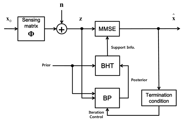
CS-BSD has a detection-directed (DD) estimation structure which consists of signal support detection and signal value estimation, as shown in Fig.1. We consider the common procedure of first using the measurements at hand to detect the signal’s support set. This detected support set is then used in the model of the sparse signal, and the value estimator is built as if the detected support set is in fact the correct set. The support detection component consists of a combination of the Bayesian hypothesis test (BHT) and BP, and signal value estimation using the detected support set is achieved via an MMSE estimator. CS-BSD iterates the detection and estimation processes until the constraint in (3) is met.

The DD estimation methodology was investigated in [21] for estimation of noisy signals and have been widely applied to wireless communication systems [22],[23]. For CS, the methodology was first reported in [24],[25]; we tailor the methodology to the NCS problem by refining that work. The complexity of CS-BSD is $O(N\log N+KM)$ whereas that of the other BP-based algorithm is $O(N\log N)$ because CS-BSD includes the cost of MMSE in addition to that of BP. However, CS-BSD converges faster than the other BP-based algorithms; thus, its computational cost is lower in practice. In addition, CS-BSD can be much faster by converting to an parallel architecture.

The rest of the paper is organized as follows. Section II introduces the sparse sensing matrix, the prior model for our system model. The details of CS-BSD are given in Section III. A few practical issues are discussed in Section IV. We compare the numerical results of CS-BSD to the other recent CS algorithms in Section V. Section VI concludes the paper.

II System Model

II-A Sparse Sensing Matrix $\mathbf{\Phi}$

For signal sensing, we employ sparse-Bernoulli matrices $\mathbf{\Phi}\in\{0,1,-1\}^{M\times N}$, which have been successfully used in CS recently [12]-[14]. In the matrix, sparsely nonzero elements are equiprobably equal to $1$ or $-1$. We set the sparsity of $\mathbf{\Phi}$ using the fixed column weight $L$. Because the column weight rather than the row weight is fixed, all elements of $\mathbf{x}_{0}$ have an even chance of being sensed. In addition, the fixed column weight unifies the energy of the basis of the measurement space spanned by the column vectors of $\mathbf{\Phi}$.

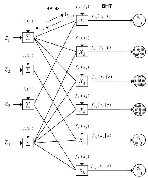
With the sparse-Bernoulli matrix, the linear system $\mathbf{z}=\mathbf{\Phi}\mathbf{x}_{0}+\mathbf{n}$ can be represented over a bipartite graph. Let $\mathcal{V}:=\{1,2,...,N\}$ denote a set of indices corresponding to the elements of the signal vector, $\mathbf{x}_{0}=[x_{0,1},x_{0,2},...,x_{0,N}]$. Similarly, $\mathcal{C}:=\{1,2,...,M\}$ denotes a set of indices corresponding to the elements of the measurement vector, $\mathbf{z}=[z_{1},z_{2},...,z_{M}]$. In addition, we define a set of edges connecting $\mathcal{V}$ and $\mathcal{C}$ as $\mathcal{E}:=\{(i,j)\in\mathcal{V}\times\mathcal{C}\,|\,\,|\phi_{ij}|=1\}$ where $\phi_{ij}$ is the $(i,j)$-th element of $\mathbf{\Phi}$. Then, A bipartite graph $\mathcal{G}:=(\mathcal{V,C,E})$ fully describes the neighboring relation in the linear system. Furthermore, we define the neighbor set of $\mathcal{V}$ and $\mathcal{C}$ as $N_{\mathcal{V}}(i):=\{j\in\mathcal{C}\,|(i,j)\in{\mathcal{E}}\}$ for all $i\in\mathcal{V}$ and $N_{\mathcal{C}}(j):=\{i\in\mathcal{V}\,|(i,j)\in{\mathcal{E}}\}$ for all $j\in\mathcal{C}$, respectively. Note that $\left|N_{\mathcal{V}}(i)\right|=L$ for all $i\in\mathcal{V}$ under our assumption regarding $\mathbf{\Phi}$. Fig.2 depicts a simple example of the graphical representation corresponding to $N=6,M=4,L=2$.

II-B Prior Model

We limit our discussion to the random vector $\mathbf{x}$ whose elements are i.i.d. random variables. This assumption is commonly used in many papers [7]-[15]. We characterize the signal sparsity in a probabilistic manner, called sparsity rate. The sparsity rate $q$ is defined as $q:=\Pr\{x_{i}\neq 0\}$ for all $i\in\mathcal{V}$. Namely, each signal element independently belongs to the signal support set with the rate $q$. The supportiveness of each signal element is represented by a state variable $s_{i}$, defined as

$${s_{i}}=\left\{\begin{array}[]{l}1,\,\,\,\,\,{\rm{if}}\,\,{x_{i}}\neq 0\\ 0,\,\,\,\,\,{\rm{else}}\end{array}\right.\text{ for all }\,\,i\in\mathcal{V}.$$ (6)

Hence, we model the prior density of $x_{i}$ using a spike-and-slab model originating in a two-state mixture density as follows:

$$f_{x}(x) := qf_{x}(x|s=1)+(1-q)f_{x}(x|s=0)$$ (7)

$$= q\mathcal{N}(x;0,\sigma_{x}^{2})+(1-q)\delta(x),$$

where $\delta(x)$ indicates a Dirac distribution having nonzero value between $x\in[0-,0+]$ and $\int\delta(x)dx=1$. In the prior density, we use Gaussian density $\mathcal{N}(x;0,\sigma_{x}^{2})$ for $f_{x}(x|s=1)$ although it includes the probability mass at $x_{i}=0$. The reason is the probability mass at $x_{i}=0$ is very small and Gaussian densities are mathematically tractable. In addition, we drop the index $i$ from the prior density under the assumption of i.i.d. elements. The spike-and-slab prior has been widely employed in Bayesian inference problems [26]-[28] and was recently applied to CS [11] as well.

III Proposed Algorithm

In this section, we discuss the details of the proposed algorithm based on the DD estimation structure. The proposed algorithm, CS-BSD, is an iterative algorithm that repeats the support detection and signal value estimation processes until $\mathbf{E}\left\|{{\bf{\Phi x}}-{\bf{z}}}\right\|_{2}\leq\epsilon$ is met.

III-A Detection of Support Set

The decoder detects the signal support in each element unit. Namely, the supportive state of each signal element is detected independently and converted to the support set information for the signal. First, the following simple hypothesis test can be considered for the state detection of $x_{i}$:

$$\Pr\{{x_{i}}=0|\mathbf{z}\}\mathop{\mathop{\gtrless}\limits_{{H_{1}}}}\limits^{{H_{0}}}\Pr\{{x_{i}}\neq 0|\mathbf{z}\}\text{ for all }i\in\mathcal{V},$$ (8)

where $H_{0}$ and $H_{1}$ are two possible hypotheses. If we marginalize over $s_{i}$, the left hand side of (8) becomes

$$\begin{array}[]{l}\Pr\{x_{i}=0|\mathbf{z}\}={\sum\limits_{s_{i}\in\{0,1\}}{\Pr\{x_{i}=0|\mathbf{z},s_{i}\}\Pr\{s_{i}|{\bf{z}}\}}}\\ \,\,\,\,\,\,\,\,\,\,\,\,\,\,\,\,\,\,\,\,\,\,\,\,\,\,\,\,\,\,\,\,\,\,\,=\Pr\{x_{i}=0|\mathbf{z},s_{i}=1\}\Pr\{s_{i}=1|{\bf{z}}\}+\underbrace{\Pr\{x_{i}=0|\mathbf{z},s_{i}=0\}}_{=1}\Pr\{s_{i}=0|{\bf{z}}\}\\ \,\,\,\,\,\,\,\,\,\,\,\,\,\,\,\,\,\,\,\,\,\,\,\,\,\,\,\,\,\,\,\,\,\,\,=\Pr\{x_{i}=0|\mathbf{z},s_{i}=1\}\Pr\{s_{i}=1|{\bf{z}}\}+\Pr\{s_{i}=0|{\bf{z}}\},\end{array}$$ (12)

where

$$\begin{array}[]{l}\Pr\{{x_{i}}=0|\mathbf{z},{s_{i}}=0\}=\Pr\{{x_{i}}=0|{s_{i}}=0\}\\ \,\,\,\,\,\,\,\,\,\,\,\,\,\,\,\,\,\,\,\,\,\,\,\,\,\,\,\,\,\,\,\,\,\,\,\,\,\,\,\,\,\,\,\,\,\,\,\,\,\,\,\,\,\,=\int_{0-}^{0+}{{f_{x}}({x}|{s}=0)\,d{x}}\\ \,\,\,\,\,\,\,\,\,\,\,\,\,\,\,\,\,\,\,\,\,\,\,\,\,\,\,\,\,\,\,\,\,\,\,\,\,\,\,\,\,\,\,\,\,\,\,\,\,\,\,\,\,\,=\int_{0-}^{0+}{\delta({x})\,d{x}}=1.\end{array}$$ (16)

The right hand side of (8) is

$$\begin{array}[]{l}\Pr\{x_{i}\neq 0|\mathbf{z}\}={\sum\limits_{s_{i}\in\{0,1\}}{\Pr\{x_{i}\neq 0|\mathbf{z},s_{i}\}\Pr\{s_{i}|{\bf{z}}\}}}\\ \,\,\,\,\,\,\,\,\,\,\,\,\,\,\,\,\,\,\,\,\,\,\,\,\,\,\,\,\,\,\,\,\,\,\,=\Pr\{x_{i}\neq 0|\mathbf{z},s_{i}=1\}\Pr\{s_{i}=1|{\bf{z}}\}+\underbrace{\Pr\{x_{i}\neq 0|\mathbf{z},s_{i}=0\}}_{=0}\Pr\{s_{i}=0|{\bf{z}}\}\\ \,\,\,\,\,\,\,\,\,\,\,\,\,\,\,\,\,\,\,\,\,\,\,\,\,\,\,\,\,\,\,\,\,\,\,=\Pr\{x_{i}\neq 0|\mathbf{z},s_{i}=1\}\Pr\{s_{i}=1|{\bf{z}}\},\end{array}$$ (20)

where

$$\Pr\{x_{i}\neq 0|\mathbf{z},s_{i}=0\}=\Pr\{x_{i}\neq 0|s_{i}=0\}$$ (21)

$$=\int\limits_{\mathbb{R}/\{0\}}{\delta({x})\,d{x}}=0.$$ (22)

From (12) and (20), the hypothesis test in (8) is refined as

$$\begin{array}[]{l}\frac{{\Pr\{s_{i}=0|{\bf{z}}\}}}{{\Pr\{s_{i}=1|{\bf{z}}\}}}\mathop{\mathop{\gtrless}\limits_{{H_{1}}}}\limits^{{H_{0}}}\Pr\{x_{i}\neq 0|\mathbf{z},s_{i}=1\}-\Pr\{x_{i}=0|{\bf{z}},s_{i}=1\}\\ \,\,\,\,\,\,\,\,\,\,\,\,\,\,\,\,\,\,\,\,\,\,\,\,\,\,\,\,\,\,\,\,\,\,=1-2\times\Pr\{x_{i}=0|{\bf{z}},s_{i}=1\}.\end{array}$$ (25)

Here

$$\Pr\{{x_{i}}=0|\mathbf{z},{s_{i}}=1\}=\int_{0-}^{0+}{{f_{x_{i}}}({x}|\mathbf{z},{s_{i}}=1)\,d{x}},$$ (26)

where the posterior density, $f_{x_{i}}({x}|\mathbf{z},{s_{i}}=1)$, is Gaussian because the signal and noise are assumed to be Gaussian (see p.326 in [29]). The term of $\Pr\{x_{i}=0|{\bf{z}},s_{i}=1\}$ in right hand side of (25) is caused by the use of Gaussian density $\mathcal{N}(x;0,\sigma_{x}^{2})$ for the prior of nonzero $x_{i}$. Because the variance of $f_{x_{i}}({x}|\mathbf{z},{s_{i}}=1)$ is a function of the noise variance, the probability $\Pr\{{x_{i}}=0|\mathbf{z},{s_{i}}=1\}$ is very small, and it approaches zero as the SNR increases. Therefore, we suggest setting the threshold of the hypothesis test in (25) to 1. This implies that the hypothesis test can detect the supportive state of the signal elements with a high success probability if SNR is sufficiently high.

We now describe how to obtain the probability ratio, $\frac{{\Pr\{s_{i}=0|{\bf{z}}\}}}{{\Pr\{s_{i}=1|{\bf{z}}\}}}$. By factorizing over $x_{i}$, the ratio becomes

$${\frac{{\Pr\{s_{i}=0|{\bf{z}}\}}}{{\Pr\{s_{i}=1|{\bf{z}}\}}}}={\frac{{\int{\Pr\{s_{i}=0|{\bf{z}},x_{i}\}f_{x_{i}}(x|\mathbf{z})}dx}}{{\int{\Pr\{s_{i}=1|{\bf{z}},x_{i}\}f_{x_{i}}(x|\mathbf{z})}dx}}}\mathop{\mathop{\gtrless}\limits_{{H_{1}}}}\limits^{{H_{0}}}1,$$ (27)

where $f_{x_{i}}(x|\mathbf{z})$ denotes the posterior density of $x_{i}$ given $\mathbf{z}$. The signal elements are not i.i.d. anymore given $\mathbf{z}$. In (27), $\Pr\{s_{i}|{\bf{z}},x_{i}\}=\Pr\{s_{i}|x_{i}\}$ holds true since the measurements $\mathbf{z}$ does not provide any additional information on the state given $x_{i}$. Using the Bayesian rule and the prior information, we finally obtain the hypothesis test as the following form:

$${\frac{{\Pr\{s_{i}=0|{\bf{z}}\}}}{{\Pr\{s_{i}=1|{\bf{z}}\}}}}={\frac{{\int{\frac{{f_{x}(x|s=0)\Pr\{s=0\}}}{{f_{x}(x)}}f_{x_{i}}(x|\mathbf{z})}dx}}{{\int{\frac{{f_{x}(x|s=1)\Pr\{s=1\}}}{{f_{x}(x)}}f_{x_{i}}(x|\mathbf{z})}dx}}}\mathop{\mathop{\gtrless}\limits_{{H_{1}}}}\limits^{{H_{0}}}1.$$ (28)

Since we know the prior of the state $Pr\{s\}$ from the sparsity rate, i.e., $\Pr\{s=1\}=q$, we can move the prior term to the right side, and then treat it as a threshold for the hypothesis test $\gamma:={\frac{{\Pr\{s=1\}}}{{\Pr\{s=0\}}}}={\frac{q}{(1-q)}}$. Therefore, the state of each elements can be sensed from the corresponding posterior and prior densities.

Definition 1 (BHT for state detection)

Let $\widehat{s}_{i}$ denote the detected state of $x_{i}$; $f_{x_{i}}(x|\mathbf{z})$ indicates the posterior density of $x_{i}$;, and $f_{x}(x|s)$ denotes the conditional prior density of a signal element given the state. Then, state detection for all $i\in\mathcal{V}$ is performed by choosing the hypothesis that result from

$${\frac{{\Pr\{s_{i}=0|{\bf{z}}\}}}{{\Pr\{s_{i}=1|{\bf{z}}\}}}}={\frac{{\int{\frac{{f_{x}(x|s=0)}}{{f_{x}(x)}}f_{x_{i}}(x|\mathbf{z})}dx}}{{\int{\frac{{f_{x}(x|s=1)}}{{f_{x}(x)}}f_{x_{i}}(x|\mathbf{z})}dx}}}\mathop{\mathop{\gtrless}\limits_{{H_{1}}}}\limits^{{H_{0}}}\gamma,$$ (29)

$$\text{where }\left\{\begin{array}[]{l}{H_{0}}:\widehat{s}_{i}=0\\ {H_{1}}:\widehat{s}_{i}=1\end{array}\right.,\,\,\,\gamma:=q/(1-q).$$ (32)

III-B Belief Propagation for Posterior Update

The posterior density used for the BHT is obtained and updated at every iteration via BP. Our BP process is similar to that in [12],[13] and was independently devised from [14],[15]. Distinctively, our BP process uses the information on the noise distributions $f_{n_{j}}(n)=\mathcal{N}(n;0,\sigma^{2}_{n})$ under the i.i.d. zero-mean Gaussian noise assumption.

Using Bayesian rule, we can represent the posterior density of $x_{i}$ in the form of ${\rm{Posterior=Prior}}\times\frac{{{\rm{Likelihood}}}}{{{\rm{Evidence}}}}$, given as

$$f_{x_{i}}(x|\mathbf{z})=f_{x}(x)\times\frac{{f_{\mathbf{z}}({{\bf{z}}|x_{i})}}}{f_{\mathbf{z}}(\mathbf{z})}.$$ (33)

If the sensing matrix $\mathbf{\Phi}$ is sufficiently sparse such that the corresponding bipartite graph is tree-like, we postulate that the elements of $\mathbf{z}$ associated with $x_{i}$ are independent of each other given $x_{i}$ [19]. Under the tree-like assumption, we can decompose the likelihood density $f_{\mathbf{z}}({\bf{z}}|x_{i})$ to the product of densities:

$$f_{x_{i}}(x|\mathbf{z})\propto f_{x}(x)\times\prod\limits_{j\in N(i)}f_{z_{j}}({z}|{x_{i}}).$$ (34)

We call each decomposition of the likelihood, $f_{z_{j}}(z|x_{i})$ the measurement density. Theorem 1 below demonstrates that the measurement density can be composed of the densities of the associated signal elements.

Theorem 1 (Measurement density in BP)

The measurement density $f_{z_{j}}(z|x_{i})$ is expressed as the linear convolution of all the associated distributions of the signal elements and the corresponding noise distribution $f_{n_{j}}(n)$ as follows:

$$f_{z_{j}}(z|x_{i})=\delta(z-z_{j})\otimes f_{n_{j}}(n)\otimes\left(\bigotimes\limits_{k\in N_{\mathcal{C}}(j)\backslash\{i\}}{f_{x_{k}}}(x)\right),$$ (35)

$\text{ for all }(i,j)\in\mathcal{E}$, where $\otimes$ and $\bigotimes$ are the operator for linear convolution and the linear convolution of a sequence of functions, respectively
Proof: See Appendix A.

Therefore, the essence of the BP-process is to update the signal and measurement densities by exchanging probability density messages, associated with the neighboring relation in the bipartite graph. Let $\mathbf{a}_{i\rightarrow j}$ denote the message from the $i$-th signal element to the $j$-th measurement element, called the signal message; $\mathbf{b}_{j\rightarrow i}$ is the message from the $j$-th measurement element to the $i$-th signal element, called the measurement message. The signal message is an approximation of the density of the signal element, i.e., $\mathbf{a}_{i\rightarrow j}\approx f_{x_{i}}(x|\mathbf{z})$ and it is obtained from (34) simply by replacing the measurement density with the measurement message of the previous iteration. Note that in BP-process the message coming from the $j$-th measurement is excluded in the calculation of $\mathbf{a}_{i\rightarrow j}$. Thus, the signal message at the $l$-th iteration is expressed as

$$\mathbf{a}_{i\rightarrow j}^{l}:=\eta\left[{{f_{x}}(x)\times\prod\limits_{k\in N_{\mathcal{V}}(i)\backslash\{j\}}{{\bf{b}}_{k\rightarrow i}^{l-1}}}\right]$$ (36)

$\text{ for all }(i,j)\in\mathcal{E}$, where $\eta[\cdot]$ is the normalization function to make $\int{\mathbf{a}_{i\rightarrow j}}dx=1$. Similarly, the measurement message approximates the measurement density, i.e., $\mathbf{b}_{j\rightarrow i}\approx f_{{z_{j}}}({z}|{x_{i}})$, and it is obtained from the expression of (35) by replacing the associated densities of signal elements $f_{x_{k}}(x)$ with the signal messages for the purpose of iteration , that is,

$$\mathbf{b}_{j\rightarrow i}^{l}:=\delta(z-z_{j})\otimes f_{n_{j}}(n)\otimes\left(\bigotimes\limits_{k\in N_{\mathcal{C}}(j)\backslash\{i\}}{\mathbf{a}_{k\rightarrow j}^{l}}\right).$$ (37)

The convolution operations in (37) can be efficiently computed by using the Fast fourier transform (FFT). Therefore, we express for the measurement message calculation as

$${\bf{b}}_{j\to i}^{l}:={\bf{F}}^{-1}\left[{{\bf{F}}\delta(z-z_{j})\times{\bf{F}}f_{n_{j}}(n)\times\prod\limits_{k\in N_{\mathcal{C}}(j)\backslash\{i\}}{{\bf{Fa}}_{k\to j}^{l}}}\right]$$ (38)

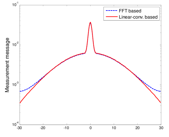
where $\mathbf{F}\in\mathbb{C}^{N_{d}\times N_{d}}$ denotes a Fourier matrix of size $N_{d}$. In fact, the use of the FFT brings a small calculation gap between this result and that of (35) since the FFT-based calculation performs a circular convolution that produces output having a heavy tail, as shown in Fig.3. The heaviness increases as the corresponding row weights in $\mathbf{\Phi}$ increase. However, the difference is can be ignored, especially when the densities are bell-shaped distributions.

Finally, the update of the posterior density of $x_{i}$ at the $l$-th iteration is provided as given in Definition 2.

Definition 2 (Posterior update in BP)

Let $\mathbf{b}_{j\rightarrow i}^{l}$ denote a measurement message at the $l$-th iteration for all $(i,j)\in\mathcal{E}$. Then, the posterior density of $x_{i}$ at the $l$-th iteration is calculated by

$$f_{x_{i}^{l}}(x|\mathbf{z})=\eta\left[{f_{x}(x)\times\prod\limits_{j\in N_{\mathcal{V}}(i)}{{\mathbf{b}_{j\rightarrow i}^{l}}}}\right],$$ (39)

where $\eta[\cdot]$ is the normalization function that makes $\int{f_{x_{i}^{l}}(x|\mathbf{z})}dx=1$.

III-C Detection-Directed Estimation of Signal Values

We now describe signal value estimation based on the DD estimation structure. The DD estimator is basically an estimator that determines how to act on the input data directed by the information from the detector. In CS-BSD, the detector provides the support information $\widehat{\mathbf{s}}^{l}$, and the value estimator then finds the signal values as if the detected support set is the correct set at each iteration. That is,

$${\widehat{\bf{x}}^{l}}=\arg\mathop{\max}\limits_{\bf{x}}{f_{\bf{x}}}({\bf{x}}|{\bf{z}},\,{\bf{s}}={\widehat{\bf{s}}}^{l})\,\,\,\,\,\,s.t.\,\,\mathbf{E}\left\|{({\bf{\Phi x}}-{\bf{z}})}\right\|_{2}\leq\epsilon,$$ (40)

where the estimator decides that $\widehat{x}_{i}^{l}=0$ for all $i\in\mathcal{V}:\widehat{s}_{i}^{l}=0$. From the argument in (25), the DD estimate converges to the true signal $\mathbf{x}_{0}$ since the detected support set becomes the correct set as SNR and the number of iterations $l$ increases. This DD methodology makes no general claim regarding optimality of the solution; however, it is common and often successful. Let $\mathbf{x}_{supp}^{l}\in\mathbb{R}^{||\widehat{\mathbf{s}}^{l}||_{0}}$ denote a random vector consisting of the elements with $\widehat{s}_{i}^{l}=1$. Then, the problem in (40) is reduced to

$$\begin{array}[]{l}\widehat{\bf{x}}_{{supp}}^{l}=\arg\mathop{\max}\limits_{{\bf{x}}}{f_{{\bf{x}}_{{supp}}^{l}}}({\bf{x}}|{\bf{z}},\,\,{\bf{s}}={\widehat{\bf{s}}}^{l})\\ =\arg\mathop{\max}\limits_{{\bf{x}}}{f_{\bf{z}}}({\bf{z}}|{\bf{x}}_{{supp}}^{l},\,{\bf{s}}={\widehat{\bf{s}}}^{l}){f_{{\bf{x}}_{{supp}}^{l}}}({\bf{x}}|{\bf{s}}={\widehat{\bf{s}}}^{l}).\end{array}$$ (43)

Since $\mathbf{x}_{supp}^{l}$ and the noise elements are assumed to be zero-mean i.i.d. Gaussian random variables with variance $\sigma_{x}^{2}$ and $\sigma_{n}^{2}$ respectively, the MAP estimation in (43) is recast as

$$\begin{array}[]{l}{\widehat{\bf{x}}_{supp}}^{l}=\arg\mathop{\min}\limits_{{\bf{x}}_{supp}^{l}}\frac{1}{{\sigma_{n}^{2}}}\left\|{{\bf{z}}-{\bf{\Phi}}_{supp}^{l}{\bf{x}}_{supp}^{l}}\right\|_{2}^{2}+\frac{1}{{\sigma_{x}^{2}}}\left\|{{\bf{x}}_{supp}^{l}}\right\|_{2}^{2},\end{array}$$ (45)

where $\mathbf{\Phi}_{supp}^{l}$ denotes a submatrix of $\mathbf{\Phi}$ corresponding to $i\in\mathcal{V}:\widehat{s}_{i}=1$. In addition, the MAP and MMSE estimates are identical, assuming the signal and noise are Gaussian (see p.358 in [29]). Therefore, the estimate $\widehat{\mathbf{x}}_{supp}^{l}$ can be obtained by the MMSE estimator

$$\widehat{\bf{x}}_{supp}^{l}=\left(\frac{1}{{\sigma_{x}^{2}}}{\bf{I}}+\frac{1}{{\sigma_{n}^{2}}}{{\bf{\Phi}}_{supp}^{l^{\,\,*}}{\bf{\Phi}}_{supp}^{l}}\right)^{-1}\frac{1}{{\sigma_{n}^{2}}}{\bf{\Phi}}_{supp}^{l^{\,\,*}}{\bf{z}}.$$ (46)

To combine the support information $\widehat{\mathbf{s}}^{l}$ and the estimated values $\widehat{\bf{x}}_{supp}^{l}$, we define an index set $\mathcal{U}^{l}:=\{1,...,{\left\|{\widehat{\bf{s}}^{l}}\right\|_{0}}\}$ corresponding to the elements $\mathbf{x}_{supp}^{l}=[x_{supp,1},...,x_{supp,{\left\|{\widehat{\bf{s}}^{l}}\right\|_{0}}}]$ and a bijective mapping function $h:\{i\in\mathcal{V}|\widehat{s}_{i}^{l}=1\}\rightarrow\mathcal{U}^{l}$. Then, the reconstruction at each iteration is readily obtained from

$$\widehat{x}_{i}^{l}=\left\{\begin{array}[]{l}\widehat{x}_{supp,h(i)}^{l},\,\,\,\,{\text{if }}\widehat{s}_{i}^{l}=1\\ 0,\,\,\,\,\,\,\,\,\,\,\,\,\,\,\,\,\,\,\,\,\,\,\,\,{\text{o.w.}}\\ \end{array}\right.$$ (49)

for all $i\in\mathcal{V}$. CS-BSD is summarized in Algorithm 1.

IV Practical issues

IV-A Complexity

We implement the BP process in CS-BSD based on the sampled-message approach in [13]. The density messages $\mathbf{a}_{i\rightarrow j},\mathbf{b}_{j\rightarrow i}$ are vectors of size $N_{d}$ where $N_{d}$ is chosen to be power of two for efficient use of FFT. Next, we analyze the complexity of CS-BSD by considering each part seperately.

IV-A1 Support detection

Let us consider the complexity of BP first. Since the matrix $\Phi$ has the fixed column weight $L$ and the size for a density vector is $N_{d}$, the decoder requires $O(LN_{d})$ flops per iteration to calculate the signal message $\mathbf{a}_{i\rightarrow j}$ in (36), and $O({\frac{{NLN_{d}}}{M}\log N_{d}})$ flops per iteration to calculate the measurement message $\mathbf{b}_{j\rightarrow i}$ in (35), since the row weight is $NL/M$ on average and the cost of the FFT-based convolution is $O(N_{d}\log N_{d})$. Hence, the per-iteration cost for all probability messages is $O(NLN_{d}+M{\frac{{NLN_{d}}}{M}\log N_{d}})$ flops. For the BHT in (29), the decoder requires $O(N_{d})$ flops to calculate a likelihood ratio. The cost for the hypothesis test is much smaller than that of BP; therefore, it is ignored.

IV-A2 Signal value estimation

Let us fix the signal sparsity as the expected value of the cardinality of the support set, i.e., $K:=E[{\left\|{{{\bf{x}}}}\right\|_{0}}]=Nq$, for purpose of comparison. Then, the complexity of the MMSE estimation in (46) depends strongly upon $K$ such that conventionally it requires $O(KM)$ flops if QR decomposition is used [30]. Thus, the total complexity of CS-BSD is $O\left(N_{iter}NLN_{d}\log N_{d}+N_{iter}KM\right)$ flops where $N_{iter}$ denotes the number of iterations. If $L$ and $N_{d}$ are fixed, the complexity of CS-BSD can be simplified to $O(N_{iter}N+N_{iter}KM)$ flops. The BP process is known to converge within $N_{iter}=O(\log N)$ [20] such that its complexity is $O(N\log N+KM\log N)$. If we fix the number of iteration $N_{iter}$ empirically, we can remove the MMSE operation from the iterations. In that case, the complexity is reduced to $O(N\log N+KM)$.

IV-B Parallelization of Belief Propagation

The BP process for finding the posterior finding can be implemented using a parallel architecture. Indeed, many parallelized BP algorithms, with applications to LDPC codes, have demonstrated superior performance in [31]-[33]. The graph representation of the sparse sensing matrix shows that the dependencies of the message calculations for any signal elements (or measurement elements) depend only upon the corresponding measurement elements (or signal elements). This allows all messages in BP to be computed in a parallel manner. Therefore, implementing BP on a parallel architecture for BP yields low power consumption, high-speed decoding, and simple logic [31].

V Numerical results

We demonstrate the advantages of CS-BSD using simulation results in several different settings. To show its average performance, we take 200 Monte Carlo trials for each point in the simulation. In each trial, we generate the deterministic sparse signal $\mathbf{x}_{0}$ with $N=1024$ and $\sigma_{x}=10$ whose values are represented with finite precision. The finite precision is provided by 6-bit quantization such that each signal value has 64 levels. This assumption of finite precision for the signal values is reasonable in terms of digital signal processing and implementation. In addition, we restrict the magnitude level of the signal elements to $|x_{i}|\leq 3\sigma_{x}$ for the same reason. We define the SNR as

$$\text{SNR :}=10\log_{10}\frac{{E{\left\|{{\bf{\Phi}}\mathbf{x}}\right\|_{2}^{2}}}}{{M\sigma_{n}^{2}}}\text{ dB }$$ (50)

and $M/N$ as the undersampling ratio for signal acquisition.

V-A SER Performance of Support Detector

To determine the performance of the support detector in CS-BSD, we defined the state error rate (SER) as:

$${\text{SER}}:=avg\left[\frac{{\#\{i\in\mathcal{V}|\widehat{s}_{i}\neq s_{0,i}\}}}{N}\right],$$ (51)

where $s_{0,i}$ is the state variable corresponding to the true signal value $x_{0,i}$. We simulate the SER performance as a function of the SNR for a variety of undersampling ratio $M/N$. In this simulation, we set $q=0.05$, $N_{d}=64$, and $L=4$. In addition. we compare the SER performance to a theoretical limit on the support recovery given by Fletcher et al. [35]. They found a necessary condition for maximum-likelihood (ML) estimation to asymptotically recover the support set if the sensing matrix has i.i.d. Gaussian entries. The ML estimation is described as

$$\mathop{\max}\limits_{\mathcal{J}}||{\bf{P}}_{\mathcal{J}}\mathbf{z}||^{2}_{2}\,\,\,\,\,\,s.t.\,\,|\mathcal{J}|={\left\|{{{\bf{x}}}}\right\|_{0}},$$ (52)

where the signal sparsity ${\left\|{{{\bf{x}}}}\right\|_{0}}$ is assumed to be known, $\mathcal{J}\subseteq\mathcal{V}$ is a subset of the index set of the signal, and ${\bf{P}}_{\mathcal{J}}\mathbf{z}$ denotes the orthogonal projection of $\mathbf{z}$ onto the subspace spanned by columns of $\mathbf{\Phi}$ corresponding to $\mathcal{J}$. Namely, the ML estimate is a subset of $\mathcal{V}$ such that the subspace spanned by the corresponding columns of $\mathbf{\Phi}$ contain the maximum energy of $\mathbf{z}$. We rewrite the necessary condition in terms of SNR such that

$$\text{SNR}>{\text{SNR}}_{limit}:=\frac{2\times{\left\|{{{\bf{x}}}}\right\|_{0}}\log(N-{\left\|{{{\bf{x}}}}\right\|_{0}})}{{(M-{\left\|{{{\bf{x}}}}\right\|_{0}}+1)\times\text{MAR}}},$$ (53)

where minimum-to-average ratio (MAR) is defined as

$$\text{MAR}:=\frac{{\mathop{\min}\limits_{j:x_{j}\neq 0}|{x_{j}}{|^{2}}}}{{\left\|{\bf{x}}\right\|_{2}^{2}/{\left\|{\bf{x}}\right\|_{0}}}}.$$ (54)

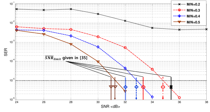
In this comparison, we used 200 Monte Carlo trials to find the average SNR_limit, i.e., $\overline{\text{SNR}}_{limit}:=avg[\text{SNR}_{limit}]$. In Fig.4, the SER curves show a waterfall behavior; the curves decline rapidly to less than $10^{-5}$ beyond a certain threshold SNR. This behavior supports the argument in (25) that the BHT achieves successful support detection in the high SNR regime. We consider the SER=$10^{-5}$ bound as an almost error-free bound since it is much less than the rate of one state error $1/N\approx 10^{-3}$ when $N=1024$. The threshold SNR for the error-free bound is roughly 34.8 dB for $M/N$=0.3, 32.9 dB for $M/N=0.4$, and 31.1 dB for $M/N=0.5$. Remarkably, this threshold SNR approaches to$\overline{\text{SNR}}_{limit}$ as $M/N$ increases. For example, the gap between the limit and the simulation result is 0.58 dB for $M/N=0.3$; however, the gap is only 0.2 dB for $M/N=0.5$. For $M/N=0.2$, since the sensing matrix $\mathbf{\Phi}$ is not sufficiently sparse, the tree-like assumption regarding $\mathbf{\Phi}$ is rarely satisfied. Such a fact occasionally causes the BP-process to diverge, leading to severe errors in support detection.

V-B MSE Performance Comparison

We consider the reconstruction performance in terms of normalized means square error (MSE), which is defined as

$${\text{MSE}}:=avg\left[\frac{{\left\|{\widehat{\bf{x}}-{\bf{x}}_{0}}\right\|_{2}^{2}}}{{\left\|{\bf{x}}_{0}\right\|_{2}^{2}}}\right].$$ (55)

We compare our algorithm to several recent CS reconstruction algorithms: 1) CS-BP [12],[13], 2) L1-DS via linear programming [5], 3) Bayesian CS (BCS) [9], 4) CoSaMP [34], and 5) SuPrEM (reweighted version) [15]. For BCS and SuPrEM, we obtained the source code from each author’s webpage; for CoSaMP we used Stephen Becker’s code (available at http://www.ugcs.caltech.edu/~srbecker/algorithms.shtml). L1-DS is provided by the L1-MAGIC package (available at http://users.ece.gatech.edu/~justin/l1magic/).We implemented CS-BP algorithm by using the sampled-message approach and upgrading the original algorithm to use the noise information. For CS-BP, we used the sparse-Bernoulli sensing matrix with $L=4$; for SuPrEM, we use a sensing matrix generated from a low-density frame [15] with the same parameters ($N$, $M$, $L$). L1-DS, CoSaMP and BCS were used with a Gaussian sensing matrix having the same column energy as the sparse-Bernoulli matrix, for fairness, i.e., $\left\|{\mathbf{\phi}_{j,Gaussian}}\right\|_{2}^{2}=\left\|{\mathbf{\phi}_{j,Sparse}}\right\|_{2}^{2}=L$. The sparsity of an input parameter in CoSaMP and SuPrEM was set according to the expectation of the cardinality of the support set $K:=E[{\left\|\mathbf{x}\right\|_{0}}]=Nq$. Those algorithms are summarized in Table I, with respect to thier complexity, type of sensing matrix, prior type, and algorithm type.

V-B1 Comparison with respect to SNR

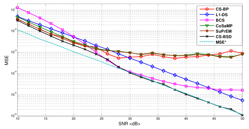
In Fig.5, we show the MSE performance as a function of SNR where $M/N=0.5$, $q=0.05$, and $N_{d}=64$. In the high SNR regime, the advantage of CS-BSD becomes remarkable. As the SNR increases, the MSE of CS-BSD approaches to that of an MMSE estimator that has knowledge of the support set, defined as

$${\text{MSE}}^{*}:=\frac{{{\rm{Tr}}\left[{\left(\frac{1}{{\sigma_{x}^{2}}}{\bf{I}}+\frac{1}{{\sigma_{n}^{2}}}{{\bf{\Phi}}_{supp}^{*}{\bf{\Phi}}_{supp}}\right)^{-1}}\right]}}{{\left\|{{\bf{x}}_{{{0,supp}}}}\right\|_{2}^{2}}},$$ (56)

where Tr$[\cdot]$ denote the matrix trace operation. Beyond SNR=31 dB, since the SER of CS-BSD is almost error-free, the MSE performance achieves ${\text{MSE}}^{*}$ at $M/N\geq 0.5$. Surprisingly, this result is superior to that of the $l_{1}$ norm based approach, which is known as an optimal algorithm in the noiseless case. The gap between the two algorithms is caused by the reconstruction error over the non-supporting elements. CS-BSD completely removes the error from the non-supporting elements whereas the $l_{1}$ norm based approach leaves a certain amount of the reconstruction error on the non-supporting elements.

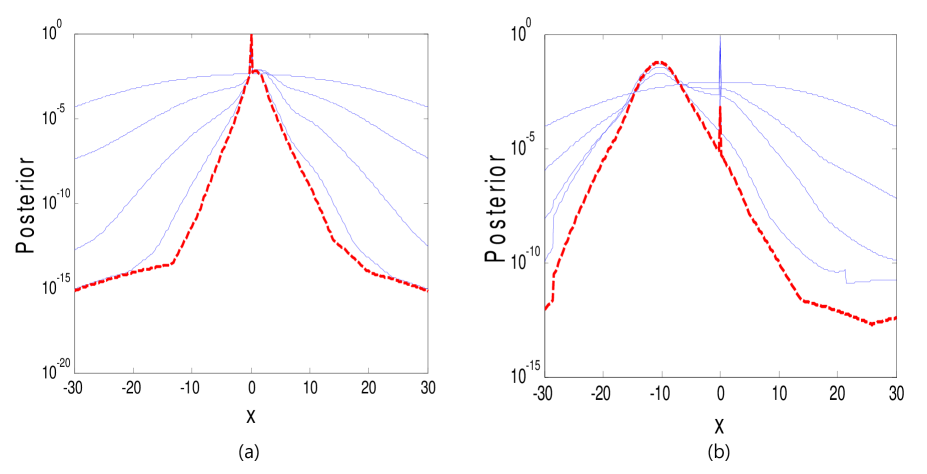
In the low SNR regime, it is noteworthy that CS-BSD works well although the proposed algorithm was originally targeted at a reasonable system having high SNR. For example, CS-BSD achieves MSE=$10^{-2}$ at SNR=14 dB in Fig.5, which provides 3 dB SNR gain from L1-DS; 2 dB gain from CoSaMP; 1 dB gain from CS-BP and SuPrEM. To support this result, we present Fig.6 which describes the iterative behavior to find the posterior of $x_{i}$ given $\mathbf{z}$ at SNR=10dB. If $s_{0,i}=0$, most of the probability mass in the posterior stays at the zero-spike as shown in Fig.6-(a); if $s_{0,i}=1$, the probability mass gradually shifts toward an estimated value as shown in Fig.6-(b), over the iteration. Since the SNR is low, the probability mass spreads considerbly over the neighbored values due to the noise effect; thus, it can lead to difficulty in detecting the state of the signal element using the simple MAP criterion. In CS-BSD, the use of the BHT nicely compensates for this weakness of the MAP by scanning the probability mass over the entire range of values.

V-B2 Comparison over number of iterations

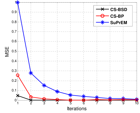
In Fig.7, we examine the MSE performance of the BP-based algorithms, CS-BP and SuPrEM, as a function of a fixed number of iterations where $N/M=0.5,q=0.1$, $N_{d}=64$, and SNR = 50 dB. In this simulation, we used the non-reweighted version of SuPrEM since the reweighted version requires more than 10 iterations. The figure demonstrates that CS-BSD converges faster than CS-BP and SuPrEM. The convergence of CS-BSD is achieved within 2 to 3 iterations with CS-BP, whereas SuPrEM require more than 10 iterations.

VI Conclusion

The theoretical and empirical research in this paper demonstrated that CS-BSD is a powerful algorithm for sparse signal reconstruction in NCS. In CS-BSD, we employed the DD estimation structure, which consists of support detection and signal value estimation. In the support detection process, BP provides the signal posterior densities, and then BHT detects the support based on the posteriors. In the signal value estimation process, an MMSE estimator provides the signal values using the detected support set. These detection and estimation process are iterated until the constraint $\mathbf{E}\|{{\bf{\Phi x}}-{\bf{z}}}\|_{2}\leq\epsilon$ is met. The evaluated SER performance showed that the support detection of CS-BSD is almost error-free beyond a certain threshold SNR according to the undersampling ratio $M/N$. On the basis of the SER result, we argued that CS-BSD achieves the performance of an MMSE estimator that has the knowledge of the support set beyond the threshold SNR. We supported the argument by evaluating the MSE performance. The complexity of CS-BSD is $O(N\log N+KM)$, which includes the cost of MMSE $O(KM)$, in addition to that of BP, $O(N\log N)$. Although our algorithm incurs an additional cost for MMSE estimation, it converges faster than other BP-based algorithms, so the computational cost is lower in practice.

Appendix A
Proof of Theorem 1

Proof: We define a random vector $\mathbf{x}_{N_{\mathcal{C}}(j)}=[x_{N_{\mathcal{C}}(j),1},...,x_{N_{\mathcal{C}}(j),W}]$ consisting of the signal elements associated with $z_{j}$ and the corresponding index set $\mathcal{W}:=\{1,...,W\}$, where $W:=|N_{\mathcal{C}}(j)|$. With a bijective mapping function $g:N_{\mathcal{C}}(j)\rightarrow\mathcal{W}$, each element of $\mathbf{x}_{N_{\mathcal{C}}(j)}$ corresponds to

$$x_{k}=x_{N_{\mathcal{C}}(j),g(k)}\text{ for all}\,\,\,k\in N_{\mathcal{C}}(j).$$ (57)

By marginalizing over $n_{j}$ to $f_{z_{j}}(z|x_{i})$, we obtain

$${f_{{z_{j}}}}({z}|{x_{i}})=\int\limits_{{n_{j}}}{{f_{{z_{j}}}}({z}|{x_{i}},{n_{j}}){f_{{n_{j}}}}({n}|{x_{i}})d{n}},$$ (58)

where ${f_{{n_{j}}}}({n}|{x_{i}})={f_{{n_{j}}}}({n})$ since $\mathbf{n}$ is independent of $\mathbf{x}$. By further marginalizing over elements of $\mathbf{x}_{N_{\mathcal{C}}(j)}$, we rewrite the expression in (58) as

$$\begin{array}[]{l}{f_{{z_{j}}}}({z}|{x_{i}})=\int\limits_{\{x_{N_{\mathcal{C}}(j),w}\}_{w=2}^{W}}\int\limits_{n_{j}}f_{z_{j}}(z|\mathbf{x}_{N_{\mathcal{C}}(j)},n_{j})f_{n_{j}}(n)f_{\mathbf{x}_{N_{\mathcal{C}}(j)}|x_{N_{\mathcal{C}}(j),1}}(x_{2},...,x_{W}|x_{i})dndx_{2}\cdots dx_{W},\\ \end{array}$$ (60)

where we assume $x_{i}=x_{N_{\mathcal{C}}(j),1}$ without loss of generality. In addition, $f_{z_{j}}(z|\mathbf{x}_{N_{\mathcal{C}}(j)},n_{j})=\delta(z-z_{j})$ holds true since knowing $\mathbf{x}_{N_{\mathcal{C}}(j)}$ is equivalent to knowing ${\left({{\bf{\Phi x}}}\right)_{row(j)}}$; thus, there is no uncertainty in $z_{j}={\left({{\bf{\Phi x}}}\right)_{row(j)}}+n_{j}$. Since the elements of $\mathbf{x}$ are assumed be independent, we replace $f_{\mathbf{x}_{N_{\mathcal{C}}(j)}|x_{N_{\mathcal{C}}(j),1}}(x_{2},...,x_{W}|x_{i})$ in (60) with the product of the probability densities.

$${f_{{z_{j}}}}({z_{j}}|{x_{i}})=\int\limits_{n_{j}}{\int\limits_{\{x_{N_{\mathcal{C}}(j),w}\}_{w=2}^{W}}{\delta(z-z_{j})f_{n_{j}}(n)\left({\prod\limits_{w=2}^{W}{f_{x_{N_{\mathcal{C}}(j),w}}(x_{w})}}(dx_{w})\right)}dn}$$ (61)

The expression in (61) can be represented by a sequence of convolutions of probability densities, as given in (35). $\,\,\,\,\,\,\,\,\,\,\,\,\,\,\,\,\,\,\,\,\,\,\,\,\,\,\,\,\,\,\,\,\,\,\,\,\,\,\,\,\,\,\,\,\,\,\,\,\,\,\,\,\,\,\,\,\,\,\,\,\,\,\,\,\,\,\,\,\,\,\,\,\,\,\,\,\,\,\,\,\,\,\,\,\,\,\,\,\,\,\,\,\,\,\,\,\,\,\,\,\,\,\,\,\,\,\,\,\,\,\,\,\,\,\,\,\,\,\,\,\,\,\,\,\,\,\,\,\,\,\,\,\,\,\,\,\,\,\,\,\,\,\,\,\,\,\,\,\,\,\,\,\,\,\,\,\,\,\,\,\,\,\,\,\,\,\,\,\,\,\,\,\,\,\,\,\,\,\,\,\,\,\,\,\,\,\,\,\,\,\,\,\,\,\,\,\,\,\,\,\,\,\,\,\,\,\,\,\,\,\,\,\,\,\,\,\,\,\,\,\,\,\,\,\,\,\,\,\,\,\,\,\,\,\,\,\,\,\,\,\,\,\,\blacksquare$

TABLE I: Comparison of several recent sparse recover algorithms

Algorithm	Complexity for recovery	Type of $\Phi$	Prior type	Algorithm type
CS-BSD	$O(N\log N+KM)$	sparse-Bernoulli	spike-and-slab	MMSE, BP, BHT
CS-BP	$O(N\log N)$	sparse-Bernoulli	two-state Gaussian mixture	MAP , BP
SuPrEM	$O(N\log N)$	Low-density frame	Jefferys’, Sparsity $K$	MAP, BP, EM
BCS	$O(NK^{2})$	Gaussian	Gamma	MAP, BP, EM,
CoSaMP	$O(MN\log K)$	Gaussian	Sparsity $K$	Greed pursuit
L1-DS	$\Omega(N^{3})$	Gaussian	-	CVX opt. via LP

Figure 1: System model of CS-BSD.

Figure 2: Overall flow of support detection in CS-BSD: A case for $N=6,M=4,L=2$.

Figure 3: Calculation gap between use of linear convolution and FFT-based convolution in measurement message calculation.

Figure 4: SER for support detection of CS-BSD over SNR for $N=1024,q=0.05$, $L=4$, and $N_{d}=64$. The double-lines indicate $\overline{\text{SNR}}_{limit}$ and the downarrow-lines denote the SNR threshold of the support detector.

Figure 5: MSE comparison over SNR for $N=1024$, $q=0.05$, $M/N=0.5$, and $N_{d}=64$ where MSE^∗ denotes the MSE of the MMSE estimator which has the support knowledge.

Figure 6: Iterative behavior to find posterior of $x_{i}$ at SNR=10dB: (a)when $s_{0,i}=0$, (b)when $s_{0,i}=1$. The dotted-red line indicates the posterior density after 5 iterations.

Figure 7: MSE performance of BP-based algorithms over the number of iterations for $N=1024,M/N=0.5,q=0.1,N_{d}=64$, and SNR = 50 dB.

Algorithm 1 CS-BSD

Noisy measurements $\mathbf{z}$, Sensing matrix $\mathbf{\Phi}$, Priori density $f_{x}(x)$, density of noise element $f_{n_{j}}(n)$.

Reconstructed signal $\widehat{\mathbf{x}}$, Detected support set $\widehat{\mathbf{s}}$.

1)Initialization:

set $l=0$, $\epsilon$

set $\mathbf{b}_{j\rightarrow i}^{l=0}=\mathbf{1}\text{ for all }(i,j)\in\mathcal{E}$

set $\gamma=q/(1-q)$

while  $\mathbf{E}\|{{\bf{\Phi}}{\bf{x}}^{l}-{\bf{z}}}\|_{2}>\epsilon$ do

     set $l=l+1$

     2)Support Detection:

     set ${\mathbf{a}}_{i\rightarrow j}^{l}=\eta[{f_{x}(x)\times\prod\limits_{k\in N_{\mathcal{V}}(i)\backslash\{j\}}{{\bf{b}}_{k\rightarrow i}^{l-1}}}]$, and $\,\,\,\,\,\,\mathbf{b}_{j\rightarrow i}^{l}:=\delta(z-z_{j})\otimes f_{n_{j}}(n)\otimes\left(\bigotimes\limits_{k\in N_{\mathcal{C}}(j)\backslash\{i\}}{\mathbf{a}_{k\rightarrow j}^{l}}\right)$ $\,\,\,\,\text{ for all }(i,j)\in\mathcal{E}$

     set $f_{x_{i}^{l}}(x|\mathbf{z})=\eta\left[{f_{x}(x)\times\prod\limits_{j\in N_{\mathcal{V}}(i)}{{\mathbf{b}_{j\rightarrow i}^{l}}}}\right]\text{ for all }i\in\mathcal{V}$

     for $i=1$ to $N$ do

         if ${\frac{{\int{\frac{{f_{x}(x|s=0)}}{{f_{x}(x)}}f_{x_{i}^{l}}(x|\mathbf{z})}dx}}{{\int{\frac{{f_{x}(x|s=1)}}{{f_{x}(x)}}f_{x_{i}^{l}}(x|\mathbf{z})}dx}}}<\gamma$ then set $\widehat{s}_{i}^{l}=1$

         else set $\widehat{s}_{i}^{l}=0$

         end if

     end for

     set $\mathbf{\Phi}_{supp}^{l}(\widehat{\mathbf{s}}^{l})$

     3)Signal Value Estimation:

     set $\widehat{\bf{x}}_{supp}^{l}=\left(\frac{1}{{\sigma_{x}^{2}}}{\bf{I}}+\frac{1}{{\sigma_{n}^{2}}}{{\bf{\Phi}}_{supp}^{l^{\,\,*}}{\bf{\Phi}}_{supp}^{l}}\right)^{-1}{\bf{\Phi}}_{supp}^{l^{\,\,*}}\frac{1}{{\sigma_{n}^{2}}}{\bf{z}}$

     set $\widehat{x}_{i}^{l}=\left\{\begin{array}[]{l}\widehat{x}_{supp,h(i)}^{l},\,\,\,\,{\text{if }}\widehat{s}_{i}=1\\ 0,\,\,\,\,\,\,\,\,\,\,\,\,\,\,\,\,\,\,\,\,\,\,\,\,{\text{o.w. }}\\ \end{array}\right.$ $\text{ for all }i\in\mathcal{V}$

end while

References

• [1] D. L. Donoho, M. Elad, and V. Temlyakov, ”Stable recovery of sparse overcomplete representations in the presence of noise,” IEEE Trans. Inf. Theory, vol. 52, no. 1, pp. 6-18, Jan. 2006.
• [2] E. Candes, J. Romberg, and T. Tao, ”Stable signal recovery from incomplete and inaccurate measurements,” Comm. Pure Appl. Math., vol. 59, no. 8, pp. 1207-1223, Aug. 2006.
• [3] J. A. Tropp, ”Just relax: Convex programming methods for identifying sparse signals in noise,” IEEE Trans. Inf. Theory, vol. 52, no. 3, pp. 1030-1051, 2006.
• [4] J. Haupt and R. Nowak, ”Signal reconstruction from noisy random projections,” IEEE Trans. Inf. Theory, vol 52, no. 9, 4036-4048, Sep. 2006.
• [5] E. Candes and T. Tao, ”The Dantzig selector: Statistical estimation when p is much larger than n,” Ann. Statist., vol. 35, no. 6, pp. 2313-2351, 2007.
• [6] D. L. Donoho and M. Elad, ”Optimally sparse representation in general dictionaries via l1 minimization,” Proc. Nat. Sci. (PNAS), vol. 100, no. 5, pp. 2197-2002, Mar. 2003.
• [7] M. E. Tipping, ”Sparse Bayesian learning and the relevance vector machine,” J. Mach. Learn. Res., vol. 1, pp. 211-244, 2001.
• [8] D. P. Wipf and B. D. Rao, ”Sparse Bayesian learning for basis selection,” IEEE Trans. Signal Process., vol. 52, no. 8, pp. 2153-2164, Aug. 2004.
• [9] Shihao Ji, Ya Xue, and Lawrence Carin, ”Bayesian compressive sensing,” IEEE Trans. Signal process., vol. 56, no. 6, pp. 2346-2356, June. 2008. (The MATLAB code is available at http://people.ee.duke.edu/~lcarin/BCS.html.)
• [10] S. Babacan, R. Molina, and A. Katsaggelos, ”Bayesian compressive sensing using Laplace priors,” IEEE Trans. Signal Process., vol. 19, no. 1, pp. 53-63, Jan. 2010.
• [11] L. He, L. Carin, ”Exploiting structure in wavelet-based Bayesian compressive sensing,” IEEE Trans. Signal Process., vol. 57, no. 9, pp. 3488-3497, Sep. 2009.
• [12] S. Sarvotham, D. Baron, and R. Baraniuk, ”Compressed sensing reconstruction via belief propagation,” Rice Univ., Houston, TX, Tech. Rep. TREE0601, Jul. 2006.
• [13] D. Baron, S. Sarvotham, and R. Baraniuk, ”Bayesian compressive sensing via belief propagation,” IEEE Trans. Signal Process., vol. 58, no. 1, pp. 269-280, Jan. 2010.
• [14] X. Tan and J. Li, ”Computationally efficient sparse Bayesian learning via belief propagation,” IEEE Trans. Signal Process., vol. 58, no. 4, pp. 2010-2021, Apr. 2010.
• [15] M. Akcakaya, J. Park, and V. Tarokh, ”A coding theory approach to noisy compressive sensing using low density frame,” accepted to IEEE Trans. Signal Process., 2011. (The MATLAB code is available at http://people.fas.harvard.edu/~akcakaya/suprem.html)
• [16] D. Andrews and C. Mallows, ”Scale mixtures of normal distributions,” J. R. Stat. Soc., vol. 36, pp. 99-102, 1974.
• [17] M. A. T. Figueiredo and R. Nowak, ”Wavelet-based image estimation: An empirical bayes approach using Jeffreys noninformative prior,” IEEE Trans. Image Proc., vol. 10, pp. 1322-1331, Sep. 2001.
• [18] R. G. Gallager, Low-Density Parity Check Codes, MIT Press: Cambridge, MA, 1963.
• [19] T. Richardson, and R. Urbanke, ”The capacity of low-density parity check codes under message-passing decoding,” IEEE Trans. Inform. Theory, vol. 47, no. 2, pp. 599-618, Feb. 2001.
• [20] D. MacKay, ”Good error-correcting codes based on very sparse matrices,”IEEE Trans. Inf. Theory, vol. 45, no. 2, pp. 399-431, Mar. 1999.
• [21] D. Middleton and R. Esposito, ”Simultaneous optimum detection and estimation of signal in noise,” IEEE Trans. Inform. Theory, vol. 14, no. 3, pp. 434-444, May. 1968.
• [22] G. Picchi and G. Prati, ”Blind equalization and carrier recovery using ”Stop-and-Go” decision-directed algorithm,” IEEE Tran. Communi., vol. 35, no. 9, pp. 877-887, Sep. 1987.
• [23] D. Godard, ”Self-recovering equalization and carrier tracking in two-dimensional data communication systems,”IEEE Tran. Communi., vol. 28, no. 11, pp. 1867-1875, Nov. 1980.
• [24] Heung-No Lee, Introduction to Compressed Sensing (Lecture notes), Spring Semester, 2011.
• [25] Jaewook Kang, Heung-No Lee, and Kiseon Kim, ”Message Passing Aided Least square Recovery for Compressive Sensing,” in Proc. Signal Processing with Adaptive Sparse Structured Representation (SPARS), pp. 124, Jun. 2011.
• [26] H. Ishwaran and J. S. Rao, ”Spike and slab variable selection : Frequentist and Bayesian strategies,” Ann. Statist., vol.33, pp. 730-773, 2005.
• [27] E. I. George and R. E. McCulloch, ”Variable selection via Gibbs sampling,” J. Amer. Statist. Assoc., vol. 88, pp. 881-889, 1993.
• [28] C. Carvalho, J. Chang, J. Lucas, Q. Wang, J. Nevins, and M. West, ”High-dimensional sparse factor modelling: Applications in gene expression genomics,” J. Amer. Statist. Assoc., 2008.
• [29] S. Kay, Fundamentals of Statistical Signal Processing Volume I: Estimation theory, Prentice Hall PTR, 1993.
• [30] Ake Bjorck, Numerical Methods for Lesast Squares Problems,,SIAM: PA, 1996.
• [31] C. Howland, A. Blanksby, ”Parallel decoding architectures for low density parity check codes,” in Proc. IEEE Int. Symp. on Circ. and Syst. (ISCAS), pp. 742- 745, May 2001.
• [32] K. Shimizu, T. Ishikawa, N. Togawa, T. Ikenaga, and S. Goto, ”A parallel LSI architecture for LDPC decoder improving message-passing schedule,” in Proc. IEEE Int. Symp. on Circ. and Syst. (ISCAS), pp. 5099-5102, May 2006
• [33] S. Wang, S. Cheng, and Q. Wu, ”A parallel decoding algorithm of LDPC codes using CUDA,” in proc. 42th Asilomar Conference on Signals, Systems and Computers, pp. 171-175, 2008.
• [34] D. Needell, J. Tropp, ”COSAMP: Iterative signal recovery from incomplete and inaccurate samples,” Appl. and Comput. Harmon. Anal., vol. 26, no. 3, pp. 301-321, 2008.
• [35] A. Fletcher, S. Rangan, and V. Goyal, ”Necessary and sufficient conditions for sparsity pattern recovery,” IEEE Trans. Inform. Theory, vol. 55, no. 12, pp. 5758-5772, Dec. 2009.