On the Dispersions of Three Network Information Theory Problems

Abstract

We analyze the dispersions of distributed lossless source coding (the Slepian-Wolf problem), the multiple-access channel and the asymmetric broadcast channel. For the two-encoder Slepian-Wolf problem, we introduce a quantity known as the entropy dispersion matrix, which is analogous to the scalar dispersions that have gained interest recently. We prove a global dispersion result that can be expressed in terms of this entropy dispersion matrix and provides intuition on the approximate rate losses at a given blocklength and error probability. To gain better intuition about the rate at which the non-asymptotic rate region converges to the Slepian-Wolf boundary, we define and characterize two operational dispersions: the local dispersion and the weighted sum-rate dispersion. The former represents the rate of convergence to a point on the Slepian-Wolf boundary while the latter represents the fastest rate for which a weighted sum of the two rates converges to its asymptotic fundamental limit. Interestingly, when we approach either of the two corner points, the local dispersion is characterized not by a univariate Gaussian but a bivariate one as well as a subset of off-diagonal elements of the aforementioned entropy dispersion matrix. Finally, we demonstrate the versatility of our achievability proof technique by providing inner bounds for the multiple-access channel and the asymmetric broadcast channel in terms of dispersion matrices. All our proofs are unified a so-called vector rate redundancy theorem which is proved using the multidimensional Berry-Esséen theorem.

I Introduction

Network information theory [1] aims to find the fundamental limits of communication in networks with multiple senders and receivers. The primary goal is to characterize the optimal rate region or capacity region–that is, the set of rate tuples for which there exists codes with reliable transmission. Such rate tuples are known as being achievable. While the characterization of capacity regions is a difficult problem in general, there have been positive results for several special classes of networks such as the multiple-access channel [2, 3] and the asymmetric [4] or degraded broadcast channels [5, 6]. A prominent example in multi-terminal lossless source coding in which the optimal rate region is known is the so-called Slepian-Wolf problem [7] which involves separately encoding two (or more) correlated sources and subsequently estimating them from their rate-limited representations.

The capacity region for a channel model is an asymptotic notion. One is allowed to design codes that operate over arbitrarily long blocks (or channel uses) in order to drive either the maximal or average probabilities of error to zero. To illustrate this point, let us recap Shannon’s point-to-point channel coding theorem [8]. He showed that up to $nC$ bits can be reliably transmitted over $n$ uses of a discrete memoryless channel (DMC) $W$ as $n$ becomes large. Here, $C=\max_{p_{X}}I(p_{X},W)$ is termed the capacity of the channel $W$. However, this fundamental result for reliable communication over a noisy channel can be optimistic in practice as there may be system constraints on the delay. One can thus ask a slightly different and more challenging question: What is the maximal code size $M^{*}(n,\epsilon)$ as a function of a fixed blocklength $n$ and target average error probability $\epsilon$? The second-order asymptotic behavior of $\log M^{*}(n,\epsilon)$ was studied first by Strassen [9] and the analysis was extended recently by Hayashi [10] and Polyanskiy, Poor and Verdú [11]. They showed that for most channels and for all $\epsilon\in(0,1)$,

$$\frac{1}{n}\log M^{*}(n,\epsilon)=C-\sqrt{\frac{V}{n}}\mathrm{Q}^{-1}(\epsilon)+O\left(\frac{\log n}{n}\right).$$ (1)

The constant $V$ coincides with an operational quantity known as the channel dispersion [11], which is similar to the second-order coding rate in [10]. The channel dispersion is the variance of the log-likelihood ratio of the channel $W$ and the capacity-achieving output distribution $p_{Y^{*}}$ assuming uniqueness of the capacity-achieving input distribution $p_{X^{*}}:=\operatorname*{arg\,max}_{p}I(p,W)$. The term $\sqrt{\frac{V}{n}}\,\mathrm{Q}^{-1}(\epsilon)$ is approximately the rate penalty in at blocklength $n$. The first two terms in (1) are known as the Gaussian approximation to $R^{*}(n,\epsilon)$.

In this paper, using Gaussian approximations, we ask similar dispersion-type questions for three multi-user problems: distributed lossless source coding, also known as the Slepian-Wolf (SW) problem, the multiple-access channel (MAC) and the asymmetric broadcast channel (ABC). We show that the network analogue of the scalar dispersion quantity $V$ is a positive-semidefinite matrix $\mathbf{V}$ that generally depends on the channel, input distributions or sources. We call this a global dispersion result. Furthermore, we also perform local dispersion analysis. Just as $V$ in (1) quantifies the rate of convergence of $R^{*}(n,\epsilon)$ to capacity, we examine the rate of convergence to various points on the boundary of the asymptotic rate region for the SW problem. Our results are of practical importance due to the ubiquity of communication networks where numerous users simultaneously share a data compression system or utilize a common channel. Since there may be hard constraints on the permissible number of channel uses (i.e., the delay in decoding), it is useful to gain an intuition of the approximate backoff from the asymptotic fundamental limits in terms of a quantity that is analogous to $V$ in (1).

I-A Summary of Main Results

There are three main results in this paper:

1. For the SW problem, we define the $(n,\epsilon)$-optimal rate region $\mathscr{R}_{\mathrm{SW}}^{*}(n,\epsilon)$ to be the set of rate pairs $(R_{1},R_{2})$ for which there exists a length-$n$ code such that the error probability in reconstructing the sources does not exceed $\epsilon$. We characterize $\mathscr{R}_{\mathrm{SW}}^{*}(n,\epsilon)$ up to an $O(\frac{\log n}{n})$ factor. More precisely, we show the following global dispersion result (Theorem 1) for the SW problem: $\mathscr{R}_{\mathrm{SW}}^{*}(n,\epsilon)$ is the set of rate pairs $(R_{1},R_{2})$ satisfying

   $$\begin{bmatrix}R_{1}\\ R_{2}\\ R_{1}+R_{2}\end{bmatrix}\in\begin{bmatrix}H(X_{1}|X_{2})\\ H(X_{2}|X_{1})\\ H(X_{1},X_{2})\end{bmatrix}+\frac{\mathscr{S}(\mathbf{V},\epsilon)}{\sqrt{n}}\pm O\left(\frac{\log n}{n}\right)\mathbf{1},$$ (2)

   where the set $\mathscr{S}(\mathbf{V},\epsilon)\subset\mathbb{R}^{3}$ is the multidimensional analogue of the cumulative distribution function for a zero-mean multivariate Gaussian with covariance matrix $\mathbf{V}$. See Fig. II-A for a schematic of $\mathscr{R}_{\mathrm{SW}}^{*}(n,\epsilon)$. This is pleasingly analogous to (1) in which the backoff from the asymptotic optimal rate region is of the order $O(\frac{1}{\sqrt{n}})$. The constant is also specified as the dispersion matrix $\mathbf{V}$.

2. However, while the global dispersion result for SW in (2) resembles the channel dispersion one in (1), it differs in one key aspect. Namely, the rate at which $\mathscr{R}_{\mathrm{SW}}^{*}(n,\epsilon)$ approaches certain boundary points of the asymptotic SW region is somewhat nebulous. To clarify this, we define two related operational dispersions which we also characterize exactly. First, we consider approaching various points on the boundary at a specified angle $\theta$ (See Fig. II-A). Interestingly, when we approach either of the corner points, the local dispersion (proved in Theorem 2) is characterized not by a univariate Gaussian (via the $\mathrm{Q}^{-1}$ function as in (1)) but a bivariate Gaussian, a subset of the off-diagonal elements of the dispersion matrix $\mathbf{V}$ and the angle of approach. This phenomenon is not observed when we approach non corner-points. Indeed, in this case, the local dispersion is simply characterized by an element on the diagonal of $\mathbf{V}$ and the angle of approach. Second, suppose we want to minimize a linear combination of $R_{1}$ and $R_{2}$, say $\alpha R_{1}+\beta R_{2}$ for some $\alpha,\beta\geq 0$. It can be seen from the polygonal shape of the SW region that for almost all values of $(\alpha,\beta)$, the resulting rate pairs will converge to one of the two corner points. We characterize the speed at which the $(\alpha,\beta)$-weighted sum-rate of the best SW code of length $n$ with error probability not exceeding $\epsilon$ converges to either $\alpha H(X_{1}|X_{2})+\beta H(X_{2})$ or $\alpha H(X_{1})+\beta H(X_{2}|X_{1})$. We call the proportionality constant involved in this speed the $(\alpha,\beta)$-weighted sum-rate dispersion or simply the weighted sum-rate dispersion (proved in Theorem 3).

3. Lastly, to demonstrate the full utility of our achievability proof technique which is based on the method of types [12], we apply it to obtain second-order-type inner bounds for the $(n,\epsilon)$-capacity regions for the discrete memoryless MAC (Theorem 4) and the discrete memoryless ABC (Theorem 5). These inner bounds are expressed like the global dispersion result in (2) but similar local and weighted sum-rate dispersions can also be derived.

I-B Related Work

The asymptotic expansions for the fundamental limits of hypothesis testing, source and channel coding were first studied by Strassen [9]. Subsequently, dispersion or second-order coding analysis for channel coding for various point-to-point channel models were studied in [10] and [11]. Such dispersion analysis has promptly been extended to lossy source coding [13, 14] and joint source-channel coding [15]. Dispersion analysis is complementary to that of traditional error exponent analysis [16, 12]. In the latter, we fix a rate tuple in the capacity region and ask how rapidly the error probability decays as an exponential function of the blocklength. In the former, the error probability and the blocklength are fixed (though for tractability, we often allow $n$ to also grow and we study the asymptotics). The spotlight is now shone on achievable rates at the specified blocklength and error probability.

The problem of SW coding for a fixed error probability and blocklength was discussed by Baron et al. [17], Sarvotham et al. [18] and He et al. [19]. However, in these works, the authors considered a single source $X_{1}$ to be compressed and (non-coded) side information $X_{2}$ available only at the decoder. Thus, $X_{2}$ is neither coded nor estimated. They showed that a scalar dispersion quantity governs the second-order coding rate. Thus, for this problem, we cannot observe the peculiar corner point phenomenon discussed in the second point in Section I-A. He et al. [19] also analyzed the variable-length SW problem and showed that the dispersion is, in general, smaller than in the fixed-length setting. Due to the duality between one-encoder SW coding and channel coding [20, 21, 22], this variable-length dispersion shown to be similar to that for channel coding [10, 11]. However, it is again not clear how to obtain the dispersion matrix-type result in (2) or the local and weighted sum-rate dispersions by exploiting the duality between channel coding and the one-encoder SW coding problem [20, 21]. There is also duality between the two-encoder SW problem and the MAC as stated in [12, Theorem 14.3] but it is not clear whether this duality can be exploited for deriving conclusive dispersion results for the MAC. Sarvotham et al. [23] considered the SW problem with two sources to be compressed but limited their setting to the case the sources are binary and symmetric. They demonstrated a result analogous to Baron et al. [17]. The three constraints on the individual rates $R_{1}$, $R_{2}$ and the sum rate $R_{1}+R_{2}$ are decoupled when the sources are binary and symmetric. Similar conclusions were made by Chang and Sahai [24] from an error exponent perspective. Our work generalizes their setting in that we consider all finite alphabet sources (not necessarily symmetric) with multiple encoders. We discuss further connections in Sections II-B4.

I-C Paper Organization

This paper is organized as follows: In the following subsection, we introduce our notation. In Section II, we present our dispersion results for the problem of distributed lossless source coding (the SW problem). The global dispersion result is stated first, followed by the local and weighted sum-rate dispersion results. We then provide a thorough discussion of these results, comparing and contrasting them. Following that in Sections III and IV, we present the second-order inner bounds for the MAC and ABC respectively. We conclude our discussion and suggest avenues for further research in Section V. Most of the proofs are presented in Section VI where we start by presenting a general result known as the vector rate redundancy theorem. We subsequently apply it in the achievability proofs for the SW problem, the MAC and the ABC. The proofs of the local and weighted sum-rate dispersion results are presented in the appendices, together with other auxiliary results.

I-D Notation

We adopt the following set of notation: Random variables and the values they take on will be denoted by upper case (e.g., $X$) and lower case (e.g., $x$) respectively. Random vectors will be denoted by upper case bold font or with a superscript indicating its length (e.g., $\mathbf{X}$ or $X^{n}=(X_{1},\ldots,X_{n})$). Their realizations will be denoted by lower case bold font or with a superscript (e.g., $\mathbf{x}$ or $x^{n}=(x_{1},\ldots,x_{n})$). Matrices will also be denoted by upper case bold font (e.g., $\mathbf{M}$); this should hopefully cause no confusion with random vectors. The notation $\mathbf{M}^{T}$ denotes the transpose of $\mathbf{M}$. The notations $\mathbf{M}\succ 0$ and $\mathbf{M}\succeq 0$ mean that $\mathbf{M}$ is (symmetric) positive-definite and positive-semidefinite respectively. In addition, $\lambda_{\min}(\mathbf{M})$, $\lambda_{\max}(\mathbf{M})$ and $\|\mathbf{M}\|_{2}$ denote, respectively, the minimum and maximum eigenvalue and the spectral norm of $\mathbf{M}$. The $(i,j)$ element of $\mathbf{M}$ is denoted as $[\mathbf{M}]_{i,j}$. For a vector $\mathbf{v}\in\mathbb{R}^{d}$, $\|\mathbf{v}\|_{q}=(\sum_{t=1}^{d}|v_{t}|^{q})^{1/q}$ is the $\ell_{q}$ norm for $q\in[1,\infty]$. The notation $\mathbf{1}$ denotes the vector of all ones. For two vectors $\mathbf{u},\mathbf{v}\in\mathbb{R}^{d}$, $\mathbf{u}\leq\mathbf{v}$ means $u_{t}\leq v_{t}$ for all $t=1,\ldots,d$. The notation $\mathbf{u}\geq\mathbf{v}$ is defined similarly. Sets will be denoted by calligraphic font (e.g., $\mathcal{X}$). Subsets of Euclidean space will be denoted by script font (e.g., $\mathscr{R}$).

Types (empirical distributions) will be denoted by upper case (e.g., $P$) and distributions by lower case (e.g., $p$). The set of distributions supported on a finite set $\mathcal{X}$ and the set of $n$-types supported on $\mathcal{X}$ will be denoted by $\mathscr{P}(\mathcal{X})$ and $\mathscr{P}_{n}(\mathcal{X})$ respectively. The type of a sequence $x^{n}$ is denoted as $P_{x^{n}}$. The set of all sequences whose type is some $P$ is denoted as $\mathcal{T}_{P}$, the type class. For two sequences $x^{n}\in\mathcal{X}^{n},y^{n}\in\mathcal{Y}^{n}$, the conditional type of $y^{n}$ given $x^{n}$ is the stochastic matrix $V:\mathcal{X}\to\mathcal{Y}$ satisfying $P_{x^{n}}(a)V(b|a)=P_{x^{n},y^{n}}(a,b)$ for all $(a,b)\in\mathcal{X}\times\mathcal{Y}$. The set of $y^{n}$ with conditional type $V$ given $x^{n}$ is denoted by $\mathcal{T}_{V}(x^{n})$, the $V$-shell of $x^{n}$. The family of stochastic matrices $V:\mathcal{X}\to\mathcal{Y}$ for which the $V$-shell of a sequence $x^{n}\in\mathcal{T}_{P}$ is not empty is denoted as $\mathscr{V}_{n}(\mathcal{Y};P)$ [12, Sec. 2.5].

Entropy and conditional entropy are denoted as $H(X)=H(p_{X})$ and $H(Y|X)=H(p_{Y|X}|p_{X})$ respectively. Mutual information is denoted as $I(X;Y)=I(p_{X},p_{Y|X})$. We often times make the dependence on the distribution explicit. Let $x^{n},y^{n}$ be a pair of sequences for which the $y^{n}$ has conditional type $V$ given $x^{n}$ and let $\tilde{X}$ and $\tilde{Y}$ be dummy random variables with joint distribution $P_{x^{n},y^{n}}$. Then, the notations $\hat{H}(x^{n})=H(P_{x^{n}})=H(\tilde{X})$ and $\hat{H}(y^{n}|x^{n})=H(V|P_{x^{n}})=H(\tilde{Y}|\tilde{X})$ denote, respectively, the empirical marginal and conditional entropies respectively. Note that empirical information quantities will generally be denoted with hats. So for example, the empirical mutual information of the random variables $\tilde{X},\tilde{Y}$ above will be denoted interchangeably as $\hat{I}(x^{n}\wedge y^{n})=I(P_{x^{n}},V)=I(\tilde{X};\tilde{Y})$. Empirical conditional mutual information is defined similarly.

The multivariate Gaussian probability density function with mean $\mathbf{m}$ and covariance $\bm{\Lambda}$ is denoted as $\mathcal{N}(\mathbf{u};\mathbf{m},\bm{\Lambda})$ or more simply as $\mathcal{N}(\mathbf{m},\bm{\Lambda})$. For a standard univariate Gaussian $\mathcal{N}(u;0,1)$, the cumulative distribution function and $\mathrm{Q}$-function are defined as $\Phi(z):=\int_{-\infty}^{z}\mathcal{N}(u;0,1)\,\mathrm{d}u$ and $\mathrm{Q}(z):=1-\Phi(z)$ respectively. The functional inverse of the $\mathrm{Q}$-function is denoted as $\mathrm{Q}^{-1}(\epsilon)$. The Bernoulli random variable $X\sim\mathrm{Bern}(q)$ if $\mathsf{P}(X=1)=q$ and $\mathsf{P}(X=0)=1-q$. Logarithms are to the base 2. We also use the discrete interval notation $[2^{nR}]:=\{1,\ldots,\lceil{2^{nR}}\rceil\}$. Asymptotic notation such as $o(\,\cdot\,),O(\,\cdot\,)$ and $\Theta(\,\cdot\,)$ is used throughout. See [25, Sec. I.3] for definitions.

II Dispersion of Distributed Lossless Source Coding

Distributed lossless source coding—also known as the Slepian-Wolf or SW problem—consists in separately encoding two (or more) correlated sources $(X_{1}^{n},X_{2}^{n})\sim\prod_{k=1}^{n}p_{X_{1},X_{2}}(x_{1k},x_{2k})$ into a pair of rate-limited messages $(M_{1},M_{2})\in[2^{nR_{1}}]\times[2^{nR_{2}}]$. Subsequently, given these compressed versions of the sources, a decoder seeks to reconstruct $(X_{1}^{n},X_{2}^{n})$. One of the most remarkable results in information theory, proved by Slepian and Wolf in 1973 [7], states that the set of achievable rate pairs $(R_{1},R_{2})$ is asymptotically equal to that when each of the encoders is also given knowledge of the other source, i.e., encoder 1 knows $X_{2}^{n}$ and vice versa. The optimal rate region $\mathscr{R}_{\mathrm{SW}}^{*}$ is given by the polyhedron

$$R_{1} \geq H(X_{1}|X_{2})$$ (3a)

$$R_{2} \geq H(X_{2}|X_{1})$$ (3b)

$$R_{1}+R_{2} \geq H(X_{1},X_{2}).$$ (3c)

We are also interested in the optimal weighted sum-rate; that is, for constants $\alpha,\beta\geq 0$, the minimum value of $\alpha R_{1}+\beta R_{2}$ for achievable $(R_{1},R_{2})$. Of particular interest is the case $\alpha=\beta=1$, corresponding to the standard sum-rate, but other cases may be important as well, such as if transmitting from encoder 1 is more costly than transmitting from encoder 2. Because of the polygonal shape of the optimal region described in (3), the optimal weighted sum-rate is always achieved at one of the two corner points, and the optimal rate is given by

$$R_{\text{sum}}^{*}(\alpha,\beta):=\begin{cases}\alpha H(X_{1}|X_{2})+\beta H(X_{2})&\alpha\geq\beta\\ \alpha H(X_{1})+\beta H(X_{2}|X_{1})&\alpha<\beta.\end{cases}$$ (4)

As with most other statements in information theory [12], the results in (3) and (4) are first-order asymptotic. In this section, we analyze the second-order, or dispersion behavior of the SW problem. That is, we study how quickly achievable rates can approach the asymptotic fundamental limits given in (3) and (4) as the blocklength grows.

We will focus on the two-sender case. A SW code is characterized by four parameters; the blocklength $n$, the rates of the first and second sources $(R_{1},R_{2})$ and the probability of error defined as

$$P_{\mathrm{e}}^{(n)}:=\mathsf{P}((\hat{X}_{1}^{n},\hat{X}_{2}^{n})\neq(X_{1}^{n},X_{2}^{n})),$$ (5)

where $\hat{X}_{1}^{n}$ and $\hat{X}_{2}^{n}$ are the reconstructed versions of $X_{1}^{n}$ and $X_{2}^{n}$ respectively. Each blocklength $n$ and probability of error $\epsilon\in(0,\frac{1}{2})$ results in some achievable region of rate pairs that will in general be smaller than the asymptotically optimal region $\mathscr{R}_{\mathrm{SW}}^{*}$ (for $\epsilon\in(\frac{1}{2},1)$, the achievable region will, in general, be larger). Our first result in this section is a characterization of the $(n,\epsilon)$-optimal region up to a $O(\frac{\log n}{n})$ correction term. This is a tight second-order result in the sense that it the gap between inner and outer bounds is $O(\frac{\log n}{n})$, and thus it exactly specifies the constants on the $O(\frac{1}{\sqrt{n}})$ terms with which the $(n,\epsilon)$-region approaches the asymptotically optimal region. However, it is a global rather than a local result, and as such it is opaque to certain behaviors about how the achievable region approaches the optimal SW boundary. To complete the story, we also define two other dispersions operationally. We characterize these dispersions exactly by leveraging the first, global result. The first is local dispersion, meaning the speed of convergence to a specific point on the boundary of the asymptotically optimal region from a specific angle. The second type of dispersion considers the weighted sum-rate discussed above: in particular, how quickly the weighted sum-rate can approach the asymptotically optimal rate given in (4).

We start with definitions followed by the statements of our results. We then discuss the implications of our results. The proof of the global result is provided in Section VI-B, and the proofs of the other dispersion results are in Appendix A.

II-A Definitions

Let $(\mathcal{X}_{1},\mathcal{X}_{2},p_{X_{1},X_{2}}(x_{1},x_{2}))$ be a discrete memoryless multiple source (DMMS). This means that $(X_{1}^{n},X_{2}^{n})\sim\prod_{k=1}^{n}p_{X_{1},X_{2}}(x_{1k},x_{2k})$, i.e., the source is independent and identically distributed (i.i.d.). We remind the reader that the alphabets $\mathcal{X}_{1},\mathcal{X}_{2}$ are finite. We also assume throughout that $p_{X_{1},X_{2}}(x_{1},x_{2})>0$ for every $(x_{1},x_{2})\in\mathcal{X}_{1}\times\mathcal{X}_{2}$ and that the sources are not independent. Finally, we assume that the error probability $0<\epsilon<1$.

Definition 1.

An $(n,2^{nR_{1}},2^{nR_{2}},\epsilon)$-SW code consists of two encoders $f_{j,n}:\mathcal{X}_{j}^{n}\to\mathcal{M}_{j}=[2^{nR_{j}}],j=1,2$, and a decoder $\varphi_{n}:\mathcal{M}_{1}\times\mathcal{M}_{2}\to\mathcal{X}_{1}^{n}\times\mathcal{X}_{2}^{n}$ such that the the error probability in (5) with $(\hat{X}_{1}^{n},\hat{X}_{2}^{n}):=\varphi_{n}(f_{1,n}(X_{1}^{n}),f_{2,n}(X_{2}^{n}))$ does not exceed $\epsilon$.

Definition 2.

A rate pair $(R_{1},R_{2})$ is $(n,\epsilon)$-achievable if there exists an $(n,2^{nR_{1}},2^{nR_{2}},\epsilon)$-SW code for the DMMS $p_{X_{1},X_{2}}(x_{1},x_{2})$. The $(n,\epsilon)$-optimal rate region $\mathscr{R}_{\mathrm{SW}}^{*}(n,\epsilon)\subset\mathbb{R}^{2}$ is the set of all $(n,\epsilon)$-achievable rate pairs.

Definition 3.

A weighted sum-rate $R_{\textrm{sum}}$ is $(n,\epsilon,\alpha,\beta)$-achievable if there exists an $(n,\epsilon)$-achievable pair $(R_{1},R_{2})$ such that $\alpha R_{1}+\beta R_{2}\leq R_{\text{sum}}$. Let $R_{\text{sum}}^{*}(n,\epsilon;\alpha,\beta)$ be the minimum $(n,\epsilon,\alpha,\beta)$-achievable sum-rate.

&         

        

(a)          (b)          (c)

Figure 1: Schematic plots of the $(n,\epsilon)$-optimal rate region $\mathscr{R}_{\mathrm{SW}}(n,\epsilon)$ for $\epsilon\leq\frac{1}{2}$ and the asymptotic SW region in (3) whose boundary is indicated by $\mathscr{B}_{\mathrm{SW}}^{*}$. We use the simplified notation $H_{1}:=H(X_{1}),H_{2}:=H(X_{2}),H_{1|2}:=H(X_{1}|X_{2})$, $H_{2|1}:=H(X_{2}|X_{1})$ and $H_{1,2}=H(X_{1},X_{2})$. The directions of approach are indicated by the arrows in the different subplots. In subplot (a), we approach the vertical boundary; the local dispersion $F(\theta,\epsilon;R_{1}^{*},R_{2}^{*})$ is given in (21). In subplot (b), we approach the sum-rate boundary; the local dispersion is given in (23). In subplot (c), we approach the corner point $(H_{1},H_{2|1})$; the local dispersion is given implicitly in (25).

Our analysis in this paper will be focused not on providing direct bounds on $\mathscr{R}_{\mathrm{SW}}^{*}(n,\epsilon)$ and $R_{\text{sum}}^{*}(n,\epsilon;\alpha,\beta)$ for finite $n$, but rather on the speed at which these approach $\mathscr{R}_{\text{SW}}^{*}$ and $R_{\text{sum}}^{*}$ respectively, as $n\to\infty$. In particular, we are interested in characterizing the quanities defined in the following two definitions. These are both versions of operational dispersion. The first is local dispersion (illustrated in Fig. II-A): the speed of convergence to a particular asymptotic rate pair from a given angle, and the second is weighted sum-rate dispersion: the speed of convergence of the weighted sum-rate for a given weight pair.

Definition 4.

Fix a rate pair $(R_{1}^{*},R_{2}^{*})$ on the boundary of the asymptotic SW rate region $\mathscr{R}_{\mathrm{SW}}^{*}$, and a probability of error $\epsilon>0$. The dispersion-angle pair $(F,\theta)$ is $(R_{1}^{*},R_{2}^{*},\epsilon)$-achievable if there exists a sequence of $(n,2^{nR_{1,n}},2^{nR_{2,n}},\epsilon)$-SW codes such that

$$\limsup_{n\to\infty}\sqrt{n}\left(R_{1,n}-R_{1}^{*}\right) \leq\sqrt{F}(\cos\theta)\mathrm{Q}^{-1}(\epsilon)$$ (6)

$$\limsup_{n\to\infty}\sqrt{n}\left(R_{2,n}-R_{2}^{*}\right) \leq\sqrt{F}(\sin\theta)\mathrm{Q}^{-1}(\epsilon).$$ (7)

The local dispersion $F(\theta,\epsilon;R_{1}^{*},R_{2}^{*})$ is the infimum of all $F$ such that $(F,\theta)$ is $(R_{1}^{*},R_{2}^{*},\epsilon)$-achievable.

Definition 5.

The weighted sum-rate dispersion for the weight pair $(\alpha,\beta)$ and probability of error $\epsilon$ is given by

$$G(\epsilon;\alpha,\beta):=\liminf_{n\to\infty}\ n\left(\frac{R_{\text{sum}}^{*}(n,\epsilon;\alpha,\beta)-R_{\text{sum}}^{*}(\alpha,\beta)}{\mathrm{Q}^{-1}(\epsilon)}\right)^{2}$$ (8)

where $R_{\text{sum}}^{*}(\alpha,\beta)$ is defined in (4).

Observe from Definition 4 that for any $\epsilon>0$, angle $\theta$, and asymptotic rate pair $(R_{1}^{*},R_{2}^{*})$, there exist codes with rates $\{(R_{1,n},R_{2,n})\}_{n\in\mathbb{N}}$ and probability of error $\epsilon$ satisfying the approximate relationships

$$R_{1,n} \approx R_{1}^{*}+\sqrt{\frac{F(\theta,\epsilon;R_{1}^{*},R_{2}^{*})}{n}}(\cos\theta)\mathrm{Q}^{-1}(\epsilon)$$ (9a)

$$R_{2,n} \approx R_{2}^{*}+\sqrt{\frac{F(\theta,\epsilon;R_{1}^{*},R_{2}^{*})}{n}}(\sin\theta)\mathrm{Q}^{-1}(\epsilon).$$ (9b)

The only interesting values of $\theta$ are those for which the rates $\{(R_{1,n},R_{2,n})\}_{n\in\mathbb{N}}$ approach the asymptotic rate pair $(R_{1}^{*},R_{2}^{*})$ from the interior (resp. exterior) of the asymptotic SW rate region $\mathscr{R}_{\mathrm{SW}}^{*}$ when $\epsilon\leq\frac{1}{2}$ (resp. when $\epsilon>\frac{1}{2}$). For example, when approaching a point on the vertical boundary [see Fig. II-A(a)], the local dispersion is only interesting if $-\frac{\pi}{2}<\theta<\frac{\pi}{2}$.

From Definition 5, for any $\epsilon>0$ and weight pair $(\alpha,\beta)$, there exists codes with rates $\{(R_{1,n},R_{2,n})\}_{n\in\mathbb{N}}$ and probability of error $\epsilon$ satisfying

$$\alpha R_{1,n}+\beta R_{2,n}\approx R_{\text{sum}}^{*}(\alpha,\beta)+\sqrt{\frac{G(\epsilon;\alpha,\beta)}{n}}\mathrm{Q}^{-1}(\epsilon).$$ (10)

Below, Theorem 2 exactly characterizes $F(\theta,\epsilon;R^{*}_{1},R^{*}_{2})$, and Theorem 3 exactly characterizes $G(\epsilon;\alpha,\beta)$.

We now define quantities that will allow us to state our results. For a positive-semidefinite symmetric matrix $\mathbf{V}\in\mathbb{R}^{d\times d}$, let the random vector $\mathbf{Z}\sim\mathcal{N}(\mathbf{0},\mathbf{V})$. Note that $\mathcal{N}(\mathbf{0},\mathbf{V})$ is a degenerate Gaussian if $\mathbf{V}$ is singular. If $\operatorname{rank}(\mathbf{V})=r<d$, all the probability mass of $p(\mathbf{u})=\mathcal{N}(\mathbf{u};\mathbf{0},\mathbf{V})$ lies in a subspace of dimension $r$ in $\mathbb{R}^{d}$. Define the set

$$\mathscr{S}(\mathbf{V},\epsilon):=\{\mathbf{z}\in\mathbb{R}^{3}:\mathsf{P}(\mathbf{Z}\leq\mathbf{z})\geq 1-\epsilon\}.$$ (11)

Note that $\mathscr{S}(\mathbf{V},\epsilon)\subset\mathbb{R}^{3}$ is well-defined even if $\mathbf{V}$ is singular. Furthermore, $\mathscr{S}(\mathbf{V},\epsilon^{\prime})\subset\mathscr{S}(\mathbf{V},\epsilon)$ if $\epsilon^{\prime}\leq\epsilon$. This set is analogous to the (inverse) cumulative distribution function of a zero-mean Gaussian with covariance matrix $\mathbf{V}$. If $\epsilon\leq\frac{1}{2}$, $\mathscr{S}(\mathbf{V},\epsilon)$ is a convex, unbounded set in the positive orthant in $\mathbb{R}^{3}$. The boundary of $\mathscr{S}(\mathbf{V},\epsilon)$ is smooth if $\mathbf{V}$ is positive-definite. We shall see that this set scaled by $\frac{1}{\sqrt{n}}$, namely $\frac{1}{\sqrt{n}}\mathscr{S}(\mathbf{V},\epsilon)$, plays an important role in specification of bounds on the $(n,\epsilon)$-optimal rate region. This set is diagrammed in two dimensions (for ease of visualization) in Fig. 2. We note that the boundaries are indeed curved due to the fact that $\mathbf{V}\succ 0$. Note that as $n$ increases to infinity or $\epsilon$ increases towards $\frac{1}{2}$, the boundaries are translated closer to the horizontal and vertical axes. If $\epsilon>\frac{1}{2}$, the region strictly includes the positive orthant. Also observe that as the condition number $\mathbf{V}$ increases, i.e., $\mathbf{V}$ tends towards being singular, the corners of the curves become “sharper” (or “less rounded”). Indeed, in the limiting case when $\mathbf{V}$ has rank one, the support of $p(\mathbf{u})=\mathcal{N}(\mathbf{u};\mathbf{0},\mathbf{V})$ belongs to a subspace of dimension one. In this case, the set $\mathscr{S}(\mathbf{V},\epsilon)$ is an axis-aligned, unbounded rectangle (a cuboid in higher dimensions). See further discussions in Section II-B4.

\begin{overpic}[width=346.89731pt]{figs/boundaries_0113} \put(25.0,27.0){\small$\frac{1}{\sqrt{n}}\mathscr{S}(\mathbf{V},\epsilon)$} \put(75.0,27.0){\small$\frac{1}{\sqrt{n}}\mathscr{S}(\mathbf{V},\epsilon)$} \end{overpic}

Figure 2: The boundaries of the region $\frac{1}{\sqrt{n}}\mathscr{S}(\mathbf{V},\epsilon)$ for different values $n$, $\epsilon$ and $\mathbf{V}$. On the left plot, $\mathbf{V}=[1\,\,\,0.01;0.01\,\,\,1]$ (small condition number) and on the right, $\mathbf{V}=[1\,\,\,0.96;0.96\,\,\,1]$ (large condition number). The regions $\frac{1}{\sqrt{n}}\mathscr{S}(\mathbf{V},\epsilon)$ lie to the top right corner of the boundaries. $\mathscr{S}(\mathbf{V},\epsilon)$ defined in (11) is a subset of $\mathbb{R}^{3}$ but in the figures, we only illustrate the projection of the set in two dimensions.

Definition 6.

The entropy density vector is defined as

$$\mathbf{h}(X_{1},X_{2}):=\begin{bmatrix}-\log p_{X_{1}|X_{2}}(X_{1}|X_{2})\\ -\log p_{X_{2}|X_{1}}(X_{2}|X_{1})\\ -\log p_{X_{1},X_{2}}(X_{1},X_{2})\end{bmatrix}.$$ (12)

The mean of the entropy density vector is the vector of entropies, i.e.,

$$\mathsf{E}[\mathbf{h}(X_{1},X_{2})]=\mathbf{H}(p_{X_{1},X_{2}}):=\begin{bmatrix}H(X_{1}|X_{2})\\ H(X_{2}|X_{1})\\ H(X_{1},X_{2})\end{bmatrix}.$$ (13)

We denote the entries of $\mathbf{H}(p_{X_{1},X_{2}})$ as $H_{t}(p_{X_{1},X_{2}})$ for $1\leq t\leq 3$. Also, let

$$\kappa:=\max_{1\leq t\leq 3}\big{\|}\nabla_{p_{X_{1},X_{2}}}^{2}H_{t}(p_{X_{1},X_{2}})\big{\|}_{2}$$ (14)

be the maximum of the spectral norms of the Hessians of $p_{X_{1},X_{2}}\mapsto H_{t}(p_{X_{1},X_{2}})$, viewed as functions of the vectorized version of $p_{X_{1},X_{2}}\in\mathbb{R}^{|\mathcal{X}_{1}||\mathcal{X}_{2}|}$.

Definition 7.

The entropy dispersion matrix $\mathbf{V}(p_{X_{1},X_{2}})$ is the covariance matrix of the random vector $\mathbf{h}(X_{1},X_{2})$ i.e., $$\mathbf{V}(p_{X_{1},X_{2}})=\operatorname{\mathsf{Cov}}(\mathbf{h}(X_{1},X_{2})).$$ (15) We abbreviate the deterministic quantities $\mathbf{H}(p_{X_{1},X_{2}})\in\mathbb{R}^{3}$ and $\mathbf{V}(p_{X_{1},X_{2}})\succeq 0$ as $\mathbf{H}$ and $\mathbf{V}$ respectively. Observe that $\mathbf{V}$ is a matrix analogue of scalar dispersion. We will find it convenient, in this and following sections, to define the non-negative rate vector $\mathbf{R}\in\mathbb{R}^{3}$ as

$$\mathbf{R}:=\begin{bmatrix}R_{1}\\ R_{2}\\ R_{1}+R_{2}\end{bmatrix}.$$ (16)

Definition 8.

Define the region $\mathscr{R}_{\mathrm{in}}(n,\epsilon)\subset\mathbb{R}^{2}$ to be the set of rate pairs $(R_{1},R_{2})$ that satisfy

$$\mathbf{R}\in\mathbf{H}+\frac{1}{\sqrt{n}}\mathscr{S}(\mathbf{V},\epsilon)+\frac{\nu\log n}{n}\mathbf{1},$$ (17)

where $\nu:=|\mathcal{X}_{1}||\mathcal{X}_{2}|+\kappa+3/2$. Also define the region $\mathscr{R}_{\mathrm{out}}(n,\epsilon)\subset\mathbb{R}^{2}$ to be the set of rate pairs $(R_{1},R_{2})$ that satisfy

$$\mathbf{R}\in\mathbf{H}+\frac{1}{\sqrt{n}}\mathscr{S}(\mathbf{V},\epsilon)-\frac{\log n}{n}\mathbf{1}.$$ (18)

Definition 9.

Define the bivariate generalization of the $\mathrm{Q}$-function as

$$\Psi(\rho;x^{\prime},y^{\prime}):=\frac{1}{2\pi\sqrt{1-\rho^{2}}}\int_{x^{\prime}}^{\infty}\int_{y^{\prime}}^{\infty}\exp\left\{-\frac{x^{2}-2\rho xy+y^{2}}{2(1-\rho^{2})}\right\}\,\mathrm{d}y\,\mathrm{d}x.$$ (19)

II-B Main Results and Interpretation

Theorem 1 (Global Dispersion for Slepian-Wolf).

Let $\epsilon\in(0,1)$. The $(n,\epsilon)$-optimal rate region $\mathscr{R}_{\mathrm{SW}}^{*}(n,\epsilon)$ satisfies

$$\mathscr{R}_{\mathrm{in}}(n,\epsilon)\subset\mathscr{R}_{\mathrm{SW}}^{*}(n,\epsilon)\subset\mathscr{R}_{\mathrm{out}}(n,\epsilon)$$ (20)

for all $n$ sufficiently large. Furthermore, the inner bound is universally attainable, i.e., the coding scheme does not depend on the knowledge of the source statistics.

The proof is provided in Section VI-B. We now state our results on the local and sum-rate dispersion. These are proved in Appendix A and hold for all $\epsilon\in(0,1)$.

Theorem 2 (Local Dispersion for Slepian-Wolf).

Let $\theta\in[0,2\pi]$. Depending on $(R_{1}^{*},R_{2}^{*})$, there are five cases:

1. $R_{1}^{*}=H(X_{1}|X_{2})$ and $R_{2}^{*}>H(X_{2})$ (vertical boundary). Then if $-\frac{\pi}{2}<\theta<\frac{\pi}{2}$,

   $$F(\theta,\epsilon;R_{1}^{*},R_{2}^{*})=\frac{[\mathbf{V}]_{1,1}}{\cos^{2}\theta}.$$ (21)

2. $R_{2}^{*}=H(X_{2}|X_{1})$ and $R_{1}^{*}>H(X_{1})$ (horizontal boundary). Then if $0<\theta<\pi$,

   $$F(\theta,\epsilon;R_{1}^{*},R_{2}^{*})=\frac{[\mathbf{V}]_{2,2}}{\sin^{2}\theta}.$$ (22)

3. $R_{1}^{*}+R_{2}^{*}=H(X_{1},X_{2})$, $R_{1}^{*}>H(X_{1}|X_{2})$ and $R_{2}^{*}>H(X_{2}|X_{1})$ (sum-rate boundary). Then if $-\frac{\pi}{4}<\theta<\frac{3\pi}{4}$,

   $$F(\theta,\epsilon;R_{1}^{*},R_{2}^{*})=\frac{[\mathbf{V}]_{3,3}}{(\cos\theta+\sin\theta)^{2}}.$$ (23)

4. $R_{1}^{*}=H(X_{1}|X_{2})$ and $R_{2}^{*}=H(X_{2})$. Then if $-\frac{\pi}{4}<\theta<\frac{\pi}{2}$, $F(\theta,\epsilon;R_{1}^{*},R_{2}^{*})$ is the solution to

   $$\Psi\left(\rho_{1,3};-\sqrt{\frac{F}{[\mathbf{V}]_{1,1}}}\,(\cos\theta)\,\mathrm{Q}^{-1}(\epsilon),-\sqrt{\frac{F}{[\mathbf{V}]_{3,3}}}\,(\cos\theta+\sin\theta)\,\mathrm{Q}^{-1}(\epsilon)\right)=1-\epsilon,$$ (24)

   where $\rho_{1,3}:=[\mathbf{V}]_{1,3}/\sqrt{[\mathbf{V}]_{1,1}[\mathbf{V}]_{3,3}}$ is the correlation coefficient of the random variables $-\log p_{X_{1}|X_{2}}(X_{1}|X_{2})$ and $-\log p_{X_{1},X_{2}}(X_{1},X_{2})$.

5. $R_{1}^{*}=H(X_{1})$ and $R_{2}^{*}=H(X_{2}|X_{1})$. Then if $0<\theta<\frac{3\pi}{4}$, $F(\theta,\epsilon;R_{1}^{*},R_{2}^{*})$ is the solution to

   $$\Psi\left(\rho_{2,3};-\sqrt{\frac{F}{[\mathbf{V}]_{2,2}}}\,(\sin\theta)\,\mathrm{Q}^{-1}(\epsilon),-\sqrt{\frac{F}{[\mathbf{V}]_{3,3}}}\,(\cos\theta+\sin\theta)\,\mathrm{Q}^{-1}(\epsilon)\right)=1-\epsilon$$ (25)

   where $\rho_{2,3}$ is defined analogously to $\rho_{1,3}$.

Theorem 3 (Weighted Sum-Rate Dispersion for Slepian-Wolf).

If $\alpha\geq\beta$, then

$$G(\epsilon;\alpha,\beta)=\min_{w_{1},w_{2}}(\alpha w_{1}+\beta w_{2})^{2}$$ (26)

where the minimum is taken over all $w_{1},w_{2}$ satisfying

$$\Psi\left(\rho_{1,3};-\frac{w_{1}\mathrm{Q}^{-1}(\epsilon)}{\sqrt{[\mathbf{V}]_{1,1}}},-\frac{(w_{1}+w_{2})\mathrm{Q}^{-1}(\epsilon)}{\sqrt{[\mathbf{V}]_{3,3}}}\right)=1-\epsilon.$$ (27)

If $\alpha<\beta$, then $G(\epsilon;\alpha,\beta)$ is also given by (26) but with the minimization subject to

$$\Psi\left(\rho_{2,3};-\frac{w_{2}\mathrm{Q}^{-1}(\epsilon)}{\sqrt{[\mathbf{V}]_{2,2}}},-\frac{(w_{1}+w_{2})\mathrm{Q}^{-1}(\epsilon)}{\sqrt{[\mathbf{V}]_{3,3}}}\right)=1-\epsilon.$$ (28)

The correlation coefficients $\rho_{1,3}$ and $\rho_{2,3}$ are as defined in Theorem 2.

II-B1 Discussion of Theorem 1

The direct part of Theorem 1 is proved using the usual random binning argument [7, 26] together with a multidimensional Berry-Essèen theorem [27]. The latter allows us to prove an important vector rate redundancy theorem (Theorem 6). This theorem is a recurring proof technique—it is also used to prove the direct parts of the analogous results for the multiple-access and broadcast channels. The decoder is a modification of a minimum empirical entropy [12] decoding rule. More precisely, we require the three empirical entropies $\hat{H}(X_{1}^{n}|X_{2}^{n})$, $\hat{H}(X_{2}^{n}|X_{1}^{n})$ and $\hat{H}(X_{1}^{n},X_{2}^{n})$ to be jointly smaller than some perturbed rate vector $\mathbf{R}-\delta_{n}\mathbf{1}$, where $\mathbf{R}$ is in the inner bound and $\delta_{n}=O(\frac{\log n}{n})$. By Taylor’s theorem, it can be seen that the empirical entropy vector behaves like a multivariate Gaussian with mean $\mathbf{H}$ and covariance $\frac{\mathbf{V}}{n}$, explaining the presence of these terms in (17) and (18). The converse is proved by leveraging on an information spectrum theorem for the SW problem by Miyake and Kanaya [28]. Also see [29, Lemma 7.2.2]. Theorem 1 extends naturally to the case where there are more than two senders.

II-B2 Comparison with Polygonal Region

We now focus on interpreting the results of Theorem 2, which provide a different perspective on the rate region. In particular, we compare the rate region with that of another source coding problem. Consider the $(n,\epsilon)$-region for lossless source coding with side information at encoders and decoder (SI-ED), also known as cooperative source coding. Specifically, first consider the problem of source coding $X_{1}$ with $X_{2}$ available as (full non-coded) side information at the encoder and the decoder. Second, we swap the roles of $X_{1}$ and $X_{2}$. Third, we consider a single-user source coding problem for the pair $(X_{1},X_{2})$. Up to $O(\frac{\log n}{n})$ terms, this region $\mathscr{R}^{*}_{\mathrm{SI-ED}}(n,\epsilon)\subset\mathbb{R}^{2}$ is the set of rate pairs $(R_{1},R_{2})$ satisfying the three scalar constraints

$$R_{1} \geq H(X_{1}|X_{2})+\sqrt{\frac{[\mathbf{V}]_{1,1}}{n}}\,\mathrm{Q}^{-1}(\epsilon)$$ (29a)

$$R_{2} \geq H(X_{2}|X_{1})+\sqrt{\frac{[\mathbf{V}]_{2,2}}{n}}\,\mathrm{Q}^{-1}(\epsilon)$$ (29b)

$$R_{1}+R_{2} \geq H(X_{1},X_{2})+\sqrt{\frac{[\mathbf{V}]_{3,3}}{n}}\,\mathrm{Q}^{-1}(\epsilon).$$ (29c)

The three decoupled constraints in (29), which describe a piecewise linear region, represent three single-user simplifications of the problem and therefore three outer bounds to $\mathscr{R}^{*}_{\mathrm{SW}}(n,\epsilon)$. The first two inequalities characterizing the region in (29) can be derived in a straightforward manner using a side information (conditional) version of Strassen’s original result [9] for hypothesis testing. The last inequality is simply one of Strassen’s original results on source coding. Also see Problem 1.1.8 in Csiszár and Körner [12] and Theorem 1 in Kontoyiannis [30].

It may appear that the piecewise linear region in (29) is very different from that described by Theorem 1. In fact, Theorem 2 asserts that these two regions differ only at the two corner points. For example, consider a rate pair approaching a point $(R_{1}^{*},R_{2}^{*})$ on the vertical boundary of the asymptotic region (i.e. $R_{1}^{*}=H(X_{1}|X_{2})$ and $R_{2}^{*}>H(X_{2})$) as in Fig. II-A(a). For the region in (29), the only relevant constraint in the neighborhood of $(R_{1}^{*},R_{2}^{*})$ is the constraint on $R_{1}$ in (29a). For the region for the full SW problem, substituting (21) into (9), we find that the best rates approaching $(R_{1}^{*},R_{2}^{*})$ from direction $\theta$ are given by the approximate relations

$$R_{1} \approx H(X_{1}|X_{2})+\sqrt{\frac{[\mathbf{V}]_{1,1}}{n}}\,\mathrm{Q}^{-1}(\epsilon)$$ (30a)

$$R_{2} \approx R_{2}^{*}+\sqrt{\frac{[\mathbf{V}]_{1,1}}{n}}\,(\tan\theta)\,\mathrm{Q}^{-1}(\epsilon).$$ (30b)

Notice that if $\theta\notin\{\pm\frac{\pi}{2}\}$ and $n$ is sufficiently large, $R_{2}$ can be made arbitrarily close to $R_{2}^{*}$, whereas the constraint on $R_{1}$ in (30a) is identical to that in (29a). That is, up to $O(\frac{\log n}{n})$ terms, achievable rates are the same as if $X_{2}$ were known perfectly at the decoder. This makes intuitive sense, since $R_{2}^{*}>H(X_{2})$, so we are in the large deviations regime for the second source $X_{2}$ and the error probability for reconstructing $X_{2}$ vanishes much more quickly than that for $X_{1}$. In fact, it vanishes exponentially fast and the exponent is the almost-lossless source coding error exponent [12, Ch. 2]. Similarly, the SI-ED and SW regions do not differ when approaching the horizontal boundary or the sum-rate boundary as in Fig. II-A(b).

However, when approaching either of the corner points, as in Fig. II-A(c), the situation is more complicated. In particular, the scalar perspective on dispersion illustrated in the region in (29) is insufficient, because characterizing the dispersions at the corner points require off-diagonal terms of the $\mathbf{V}$ matrix, as stated in (24) and (25). Intuitively, this is because there are several forces at play—for the $(H(X_{1}),H(X_{2}|X_{1}))$ point, the contribution from the marginal dispersion $[\mathbf{V}]_{2,2}$, the contribution from the sum rate dispersion $[\mathbf{V}]_{3,3}$ and also the correlation coefficient $\rho_{2,3}$. These interact to give an local dispersion that can only be expressed implicitly as in (24)–(25). Note that now the dispersion depends on the angle of approach and the correlation coefficient of $-\log p_{X_{2}|X_{1}}(X_{2}|X_{1})$ and $-\log p_{X_{1},X_{2}}(X_{1},X_{2})$ namely $\rho_{2,3}$. Hence, the off-diagonal elements of the dispersion matrix $[\mathbf{V}]_{1,3}$ and $[\mathbf{V}]_{2,3}$ are required to characterize the dispersion. However, the element $[\mathbf{V}]_{1,2}$ never appears, because there is no point at the intersection of the vertical and horizontal boundaries of the optimal rate region (for dependent sources), so they are never simultaneously at play. Hence, even though $[\mathbf{V}]_{1,2}$ is an element of the dispersion matrix, it has no impact on the local dispersion behavior.

It may at first appear that because this non-scalar dispersion behavior occurs at only two points, it is merely a curiosity, but Theorem 3 asserts that this is not the case. In particular, because the corner points are the extreme points of the optimal rate region, the behavior in their vicinity is vital to the behavior of the optimal weighted sum-rate. This is evident in the statement of Theorem 3, that in order to characterize the weighted sum-rate dispersion requires off-diagonal terms of the $\mathbf{V}$ matrix. However, the dispersion for certain pairs $(\alpha,\beta)$ reduces to that for the scalar case. In particular, if $\beta=0$, it is not hard to show (see Appendix A) using Theorem 3 that

$$G(\epsilon;\alpha,0)=\alpha^{2}[\mathbf{V}]_{1,1}.$$ (31)

Similarly, if $\alpha=0$, then

$$G(\epsilon;0,\beta)=\beta^{2}[\mathbf{V}]_{2,2}.$$ (32)

Finally, if $\alpha=\beta$, then

$$G(\epsilon;\alpha,\alpha)=\alpha^{2}[\mathbf{V}]_{3,3}.$$ (33)

Because these special cases are the only ones for which the weighted sum-rate over the asymptotic rate region is not uniquely minimized at a corner point, these results agree with the assessment that the SW region does not differ from the SI-ED region away from the corner points.

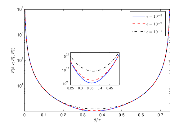
Figure 3: Plots of $F(\theta,\epsilon;R^{*}_{1},R^{*}_{2})$ against $\theta\in(0,\frac{3\pi}{4})$ for different $\epsilon$’s. This plot shows the local dispersion as we approach the corner point $(R^{*}_{1},R^{*}_{2})=(H(X_{1}),H(X_{2}|X_{1}))$ from various angles. See Fig. II-A(c) and the expression for $F(\theta,\epsilon,R^{*}_{1},R^{*}_{2})$ in (25).

II-B3 Comments on Local Dispersion at Corner Points

Interestingly, at corner points the local dispersions given by (24)–(25) depends on $\epsilon$, unlike the corresponding local dispersions for non-corner points in (21)–(23). This is illustrated numerically in Fig. 3 for the source $p_{X_{1},X_{2}}=[0.7\,\,\,0.1;0.1\,\,\,0.1]$ and the corner point $(R^{*}_{1},R^{*}_{2})=(H(X_{1}),H(X_{2}|X_{1}))$. Also, it can be seen that as $\theta\downarrow 0$, $F(\theta,\epsilon;H(X_{1}),H(X_{2}|X_{1}))$ increases without bound. This agrees with intuition because when $\theta$ is small, we are approaching the corner point almost parallel to the horizontal boundary of $\mathscr{R}_{\mathrm{SW}}(n,\epsilon)$. When $\theta\uparrow\frac{3\pi}{4}$, similarly, we are almost parallel to the sum rate boundary. On the other hand, when $\theta$ is moderate (say $\theta\approx\frac{3\pi}{8}$), the rate pair is further into the interior of $\mathscr{R}_{\mathrm{SW}}(n,\epsilon)$, hence the local dispersion is smaller. The constant $\frac{3\pi}{8}$ is in fact not arbitrary because the angle between the horizontal boundary and the sum rate boundary of $\mathscr{R}_{\mathrm{SW}}(n,\epsilon)$, is exactly $\frac{3\pi}{4}$. Hence $\frac{3\pi}{8}$ is the half-angle, which means that the rate pair is, in a sense, furthest away from either boundary. However, the smallest local dispersion does not occur at exactly $\theta=\frac{3\pi}{8}$ because of some asymmetry between the entropy densities $-\log p_{X_{1}|X_{2}}(X_{1}|X_{2})$ and $-\log p_{X_{1},X_{2}}(X_{1},X_{2})$.

The case of approaching a corner point parallel to a boundary line deserves further discussion. One may ask, for example, what trajectories of $(R_{1,n},R_{2,n})$ are achievable that approach the point $(H(X_{1}),H(X_{2}|X_{1}))$ parallel to the horizontal boundary. All we learn from Fig. 3 and from the characterization of the local dispersion is that $R_{1,n}$ must approach $H(X_{1})$ with a perturbation term larger than $O(\frac{1}{\sqrt{n}})$. This can also be observed for the case where we approach a non-corner point along the horizontal boundary of the SW region. See (22) with $\theta=0$ in which case $F(\theta,\epsilon;R_{1}^{*},H(X_{2}|X_{1}))=\infty$ for any $R_{1}^{*}>H(X_{1})$. Answering these types of questions would seem to require techniques from moderate deviations [31, 32, 33], and as such it is beyond the scope of this paper. However, we believe that our characterization of the constants on all $O(\frac{1}{\sqrt{n}})$ terms provides a good—if in this sense incomplete—portrait of the second-order behavior, and we defer this more challenging question to future work.

II-B4 Singular Entropy Dispersion Matrices

What are the implications of the $(n,\epsilon)$-SW region (Theorem 1) for singular $\mathbf{V}$’s? Note that Theorem 1 holds regardless of whether $\mathbf{V}$ is singular or positive-definite (but not for the trivial case where $\mathbf{V}=\mathbf{0}$ so we assume throughout that $\operatorname{rank}(\mathbf{V})\geq 1$). Sources for which $\mathbf{V}$ is singular include those which are (i) independent, i.e., $I(X_{1};X_{2})=0$, (ii) either $X_{1}$ or $X_{2}$ is uniform over their alphabets. It is easy to see why $I(X_{1};X_{2})=0$ results in a singular $\mathbf{V}$ — this is because the third entry in the entropy density vector is a linear combination of the first two. Thus $\mathbf{V}$ loses rank. Case (ii) was analyzed by Sarvotham et al. [23] where $X_{1},X_{2}\in\mathbb{F}_{2}$, $X_{1}\sim\mathrm{Bern}(\frac{1}{2})$, $X_{2}=X_{1}\oplus N$ with $N\sim\mathrm{Bern}(\zeta),\zeta\in(0,\frac{1}{2})$. The pair of random variables $(X_{1},X_{2})$ is the so-called discrete symmetric binary source (DSBS) with crossover probability $\zeta$. For the DSBS, Theorem 1 in [23] asserts that the $(n,\epsilon)$-optimal rate region is (up to terms in $o(\frac{1}{\sqrt{n}})$)

$$\mathbf{R}\geq\mathbf{H}+\sqrt{\frac{V_{\zeta}}{n}}\,\mathrm{Q}^{-1}(\epsilon)\mathbf{1},$$ (34)

where $V_{\zeta}$ is a scalar entropy dispersion [to be specified precisely in (35)]. Thus, the three inequalities are decoupled. In contrast, in Theorem 1, we showed that the $(n,\epsilon)$-optimal rate region for general DMMSes is such that the constraints on $R_{1}$, $R_{2}$ and $R_{1}+R_{2}$ are coupled through the set $\mathscr{S}(\mathbf{V},\epsilon)$.

Let us relate (34) to our Theorem 1. For the DSBS, it can be verified that $\operatorname{rank}(\mathbf{V})=1$ and that $\mathbf{V}$ is a scalar multiple of the all ones matrix, i.e., $\mathbf{V}=V_{\zeta}\mathbf{1}_{3\times 3}$ where $V_{\zeta}=\operatorname{\mathsf{Var}}(-\log p_{X_{1}|X_{2}}(X_{1}|X_{2}))=\operatorname{\mathsf{Var}}(-\log p_{X_{2}|X_{1}}(X_{2}|X_{1}))=\operatorname{\mathsf{Var}}(-\log p_{X_{1},X_{2}}(X_{1},X_{2}))$. Intuitively, this is because there is only one degree of freedom in a DSBS with crossover probability $\zeta$. The parameter $V_{\zeta}$ is exactly the scalar dispersion in (34). In fact, it can be calculated in closed-form for the DSBS with crossover probability $\zeta$ as

$$V_{\zeta}=\zeta(1-\zeta)\left[\log\left(\frac{1-\zeta}{\zeta}\right)\right]^{2}.$$ (35)

For this source, since $\operatorname{rank}(\mathbf{V})=1$, all the probability mass of the degenerate Gaussian $\mathcal{N}(\mathbf{0},\mathbf{V})$ lies in a subspace of dimension one. Therefore, it is easy to see that $\mathscr{S}(\mathbf{V},\epsilon)$ defined in (11) degenerates to the axis-aligned cuboid

$$\mathscr{S}(\mathbf{V},\epsilon)=\big{\{}\mathbf{z}\in\mathbb{R}^{3}:z_{t}\geq\sqrt{V_{\zeta}}\,\mathrm{Q}^{-1}(\epsilon),\forall\,1\leq t\leq 3\big{\}}.$$ (36)

The quantity $\sqrt{\frac{V_{\zeta}}{n}}\,\mathrm{Q}^{-1}(\epsilon)$ is approximately the rate redundancy [17, 18, 23, 19] for fixed-length SW coding for a DSBS. In this case, the inner and outer bounds of the $(n,\epsilon)$-optimal rate region degenerate to (34). Thus the fixed-length results in [17, 18, 23, 19] are special cases of our general result. This argument for singular dispersion matrices can be formalized and we do so in the latter half of the proof of Theorem 6.

In fact, when the dispersion matrix $\mathbf{V}$ is singular, the conclusions resulting from Theorems 2 and 3 become considerably simpler. Let us illustrate this on Theorem 2 with the DSBS with crossover probability $\zeta$ defined above. Clearly, for Theorem 2, the conclusions in (21)–(23) stay the same. However, (24) and (25) simplify to the following closed-form expressions:

$$F(\theta,\epsilon;H(X_{1}|X_{2}),H(X_{2})) =\frac{V_{\zeta}}{\cos^{2}\theta},\qquad\mbox{and}$$ (37)

$$F(\theta,\epsilon;H(X_{1}),H(X_{2}|X_{1})) =\frac{V_{\zeta}}{\sin^{2}\theta}.$$ (38)

This is because $\rho_{1,3}=\rho_{2,3}=1$ and all elements of $\mathbf{V}$ are identically equal to $V_{\zeta}$ so the two-dimensional analogue of the $\mathrm{Q}$ function, namely the $\Psi$ function defined in (19), degenerates to $\mathrm{Q}$ function evaluated at the second argument. For example, the $\Psi$ function in (24) becomes

$$\lim_{\rho\uparrow 1}\Psi\left(\rho;-\sqrt{\frac{F}{V_{\zeta}}}\,(\cos\theta)\,\mathrm{Q}^{-1}(\epsilon),-\sqrt{\frac{F}{V_{\zeta}}}\,(\cos\theta+\sin\theta)\,\mathrm{Q}^{-1}(\epsilon)\right)=\mathrm{Q}\left(-\sqrt{\frac{F}{V_{\zeta}}}\,(\cos\theta)\right),$$ (39)

which when equated to $1-\epsilon$ yields (37).

III Dispersion of the Multiple-Access Channel

The multiple-access channel or MAC is the channel coding dual to the Slepian-Wolf problem described in Section II [12, Sec. 3.2]. The MAC model has found numerous applications, especially in wireless communications where multiple parities would like to communicate to a single base station reliably. For a MAC, there are two (or more) independent messages $M_{1}\in[2^{nR_{1}}]$ and $M_{2}\in[2^{nR_{2}}]$. The two messages, which are uniformly distributed over their respective message sets, are separately encoded into sequence codewords $X_{1}^{n}\in\mathcal{X}_{1}^{n}$ and $X_{2}^{n}\in\mathcal{X}_{2}^{n}$ respectively. These codewords are the inputs to a discrete memoryless multiple-access channel (DM-MAC) $W:\mathcal{X}_{1}\times\mathcal{X}_{2}\to\mathcal{Y}$. The decoder receives $Y^{n}$ from the output of the DM-MAC and provides estimates of the messages $\hat{M}_{1}$ and $\hat{M}_{2}$ or declares that a decoding error has occurred. It is usually desired to send both messages reliably, that is, to ensure that the average probability of error

$$P_{\mathrm{e}}^{(n)}:=\mathsf{P}(\{\hat{M}_{1}\neq M_{1}\}\cup\{\hat{M}_{2}\neq M_{2}\})$$ (40)

tends to zero as $n\to\infty$. The set of achievable rates, or the capacity region $\mathscr{C}_{\mathrm{MAC}}^{*}$, is given by

$$R_{1} \leq I(X_{1};Y|X_{2},Q)$$

$$R_{2} \leq I(X_{2};Y|X_{1},Q)$$

$$R_{1}+R_{2} \leq I(X_{1},X_{2};Y|Q)$$ (41)

for some $p_{Q}$, $p_{X_{1}|Q}$ and $p_{X_{2}|Q}$ and $|\mathcal{Q}|\leq 2$. This asymptotic result was proved independently by Ahlswede [2] and Liao [3] and can be written in an alternative form which involves taking the convex hull instead of the introduction of the auxiliary time-sharing variable $Q$. See [1] for further discussions. A somewhat surprising result in the theory of MACs, which differs from point-to-point channel coding, is that the capacity region for average probability of error is strictly larger than that for maximal probability of error [34]. We emphasize that we focus on the average probability of error defined in (40) throughout. Note that as with the SW case, we can consider $\mathsf{P}(\hat{M}_{1}\neq M_{1})$, $\mathsf{P}(\hat{M}_{2}\neq M_{2})$ and $P_{\mathrm{e}}^{(n)}$ separately and place upper bounds on each of these constituent error probabilities but, for simplicity, we consider only $P_{\mathrm{e}}^{(n)}$ in (40).

In this section, we prove an inner bound to $\mathscr{C}_{\mathrm{MAC}}^{*}(n,\epsilon)$, the $(n,\epsilon)$-capacity region, when $n$ is large. This inner bound illustrates the second-order behavior of the capacity region in (41). We propose a coding scheme for a block of length $n$ that satisfies $P_{\mathrm{e}}^{(n)}\leq\epsilon$ for $n$ sufficiently large. Our encoding scheme is the coded time-sharing procedure by Han and Kobayashi [35]. The decoding scheme is similar to MMI decoding [36]. However, the error probability analysis is rather different. The result we present here is a global dispersion one (in the sense of Theorem 1) but one can define similar notions of local (Theorem 2) and sum-rate dispersion (Theorem 3) for this and the ABC problem in the following section. In a similar manner to SW, our results lead naturally to inner bounds. We do not pursue this for the MAC and ABC problems as the analysis turns out to be similar to Theorems 2 and 3.

III-A Definitions

Let $(\mathcal{X}_{1},\mathcal{X}_{2},W,\mathcal{Y})$ be a DM-MAC, i.e., for any input codeword sequences $x_{1}^{n}\in\mathcal{X}_{1}^{n}$ and $x_{2}^{n}\in\mathcal{X}_{2}^{n}$,

$$W^{n}(y^{n}|x_{1}^{n},x_{2}^{n})=\prod_{k=1}^{n}W(y_{k}|x_{1k},x_{2k}).$$ (42)

Definition 10.

An $(n,2^{nR_{1}},2^{nR_{2}},\epsilon)$-code for the DM-MAC $(\mathcal{X}_{1},\mathcal{X}_{2},W,\mathcal{Y})$ consists of two encoders $f_{j,n}:\mathcal{M}_{j}=[2^{nR_{j}}]\to\mathcal{X}_{j}^{n},j=1,2$, and a decoder $\varphi_{n}:\mathcal{Y}^{n}\to\mathcal{M}_{1}\times\mathcal{M}_{2}$ such that the average error probability defined in (40) does not exceed $\epsilon$. Note that the outputs of the encoders are $f_{j,n}(M_{j}),j=1,2$ and the output of the decoder are the estimates $(\hat{M}_{1},\hat{M}_{2})=\varphi_{n}(Y^{n})$. The coding rates are defined in the usual way.

Definition 11.

A rate pair $(R_{1},R_{2})$ is $(n,\epsilon)$-achievable if there exists an $(n,2^{nR_{1}},2^{nR_{2}},\epsilon)$-code for the DM-MAC $(\mathcal{X}_{1},\mathcal{X}_{2},W,\mathcal{Y})$. The $(n,\epsilon)$-capacity region $\mathscr{C}_{\mathrm{MAC}}^{*}(n,\epsilon)\subset\mathbb{R}^{2}$ is the set of all $(n,\epsilon)$-achievable rate pairs.

In contrast to the asymptotic setting, it is not obvious that $\mathscr{C}_{\mathrm{MAC}}^{*}(n,\epsilon)$ is convex. The usual Time Sharing argument [12, Lemma 3.2.2] — that the juxtaposition of two good multiple-access codes leads to a good but longer code — does not hold because the blocklength is constrained to be a fixed integer $n$ so juxtaposition is not allowed. Fix a triple of distributions $p_{Q}(q)$, $p_{X_{1}|Q}(x_{1}|q)$ and $p_{X_{2}|Q}(x_{2}|q)$. Given the channel $W$, these distributions induce the following output conditional distributions

$$p_{Y|X_{2},Q}(y|x_{2},q) :=\sum_{x_{1}}p_{X_{1}|Q}(x_{1}|q)W(y|x_{1},x_{2})$$ (43)

$$p_{Y|Q}(y|q) :=\sum_{x_{1},x_{2}}p_{X_{1}|Q}(x_{1}|q)p_{X_{2}|Q}(x_{2}|q)W(y|x_{1},x_{2}).$$ (44)

The output conditional distribution $p_{Y|X_{1},Q}$ is defined similarly to $p_{Y|X_{2},Q}$ with $1$ replaced by $2$ and vice versa.

Definition 12.

The information density vector is defined as

$$\mathbf{i}(Q,X_{1},X_{2},Y):=\begin{bmatrix}\log[W(Y|X_{1},X_{2})/p_{Y|X_{2},Q}(Y|X_{2},Q)]\\ \log[{W(Y|X_{1},X_{2})}/{p_{Y|X_{1},Q}(Y|X_{1},Q)}]\\ \log[{W(Y|X_{1},X_{2})}/{p_{Y|Q}(Y|Q)}]\end{bmatrix}.$$ (45)

where the distributions $p_{Y|X_{2},Q},p_{Y|X_{1},Q}$ and $p_{Y|Q}$ are defined in (43)–(44). The random variables $(Q,X_{1},X_{2},Y)$ have joint distribution $p_{Q}p_{X_{1}|Q}p_{X_{2}|Q}W$.

Observe that the expectation of the information density vector with respect to $p_{Q}p_{X_{1}|Q}p_{X_{2}|Q}W$ is the vector of mutual information quantities in (41), i.e.,

$$\mathsf{E}[\mathbf{i}(Q,X_{1},X_{2},Y)] =\mathbf{I}(p_{Q},p_{X_{1}|Q},p_{X_{2}|Q},W):=\begin{bmatrix}I(X_{1};Y|X_{2},Q)\\ I(X_{2};Y|X_{1},Q)\\ I(X_{1},X_{2};Y|Q)\end{bmatrix}.$$ (46)

Let $I_{t}(p_{Q},p_{X_{1}|Q},p_{X_{2}|Q},W)$ be the $t$-th entry of $\mathbf{I}(p_{Q},p_{X_{1}|Q},p_{X_{2}|Q},W)$. As in (14), let

$$\kappa:=\max_{1\leq t\leq 3}\left\|\nabla_{p}^{2}I_{t}(p)\right\|_{2}$$ (47)

where $p:=p_{Q,X_{1},X_{2},Y}=p_{Q}p_{X_{1}|Q}p_{X_{2}|Q}W$.

Definition 13.

The information dispersion matrix $\mathbf{V}(p_{Q},p_{X_{1}|Q},p_{X_{2}|Q},W)$ is the covariance matrix of the random vector $\mathbf{i}(Q,X_{1},X_{2},Y)$ i.e.,

$$\mathbf{V}(p_{Q},p_{X_{1}|Q},p_{X_{2}|Q},W)=\operatorname{\mathsf{Cov}}(\mathbf{i}(Q,X_{1},X_{2},Y)).$$ (48)

If there is no risk of confusion, we abbreviate the deterministic vector $\mathbf{I}(p_{Q},p_{X_{1}|Q},p_{X_{2}|Q},W)\in\mathbb{R}^{3}$ and the deterministic matrix $\mathbf{V}(p_{Q},p_{X_{1}|Q},p_{X_{2}|Q},W)\succeq 0$ as $\mathbf{I}$ and $\mathbf{V}$ respectively. We assume throughout that the channel and the input distributions are such that $\operatorname{rank}(\mathbf{V})\geq 1$, i.e., $\mathbf{V}$ is not the all-zeros matrix. Recall the definition of the rate vector $\mathbf{R}=[R_{1},R_{2},R_{1}+R_{2}]^{T}$ in (16).

Definition 14.

Given triple of input distributions $(p_{Q},p_{X_{1}|Q},p_{X_{2}|Q})$, define the region $\mathscr{R}(n,\epsilon;p_{Q},p_{X_{1}|Q},p_{X_{2}|Q})\subset\mathbb{R}^{2}$ to be the set of rate pairs $(R_{1},R_{2})$ that satisfy

$$\mathbf{R}\in\mathbf{I}-\frac{1}{\sqrt{n}}\mathscr{S}(\mathbf{V},\epsilon)-\frac{\nu\log n}{n}\mathbf{1},$$ (49)

where $\nu:=|\mathcal{Q}||\mathcal{X}_{1}||\mathcal{X}_{2}||\mathcal{Y}|+\kappa+\frac{3}{2}$. In (49), $\mathbf{I}:=\mathbf{I}(p_{Q},p_{X_{1}|Q},p_{X_{2}|Q},W)$ and $\mathbf{V}:=\mathbf{V}(p_{Q},p_{X_{1}|Q},p_{X_{2}|Q},W)$ and the set $\mathscr{S}(\mathbf{V},\epsilon)\subset\mathbb{R}^{3}$ is defined in (11).

III-B Main Result and Interpretation

Theorem 4 (Global Dispersion for DM-MAC).

Let $\epsilon\in(0,1)$. The $(n,\epsilon)$-capacity region $\mathscr{C}_{\mathrm{MAC}}^{*}(n,\epsilon)$ for the DM-MAC satisfies

$$\bigcup_{p_{Q},p_{X_{1}|Q},p_{X_{2}|Q}}\mathscr{R}(n,\epsilon;p_{Q},p_{X_{1}|Q},p_{X_{2}|Q})\subset\mathscr{C}_{\mathrm{MAC}}^{*}(n,\epsilon)$$ (50)

for all $n$ sufficiently large. Furthermore, to preserve $\mathbf{I}$ and $\mathbf{V}$, the union over $p_{Q}$ can be restricted to those discrete distributions with support $\mathcal{Q}$ whose cardinality $|\mathcal{Q}|\leq 9$. The inner bound is also universally attainable.

This theorem is proved in Section VI-C. The bounds on cardinality can be proved using the support lemma [12, Theorem 3.4]. See Section VI-C2. From (49), we see that the inner bound to the $(n,\epsilon)$-capacity region $\mathscr{C}_{\mathrm{MAC}}^{*}(n,\epsilon)$ approaches the usual MAC region (41) at a rate of $O(\frac{1}{\sqrt{n}})$ for fixed input distributions. Unsurprisingly, this rate is a consequence of the multidimensional central limit theorem. The redundancy set $\frac{1}{\sqrt{n}}\mathscr{S}(\mathbf{V},\epsilon)$ in (49) is approximately the loss in rate to the three mutual information quantities in (41) one must incur when operating at blocklength $n$ and with average error probability $\epsilon$.

For the proof of Theorem 4, we use the coded time-sharing scheme introduced by Han and Kobayashi in their seminal work on interference channels [35]. The decoding step, however, is novel and is a modification of the maximum mutual information (MMI) decoding rule [36, 12]. This MMI-decoding step allows us to define a new notion of typicality for empirical mutual information quantities. Interestingly, the error event that contributes to the $\epsilon$ probability of error is the one in which the transmitted pair of codewords $x_{1}^{n}(m_{1}),x_{2}^{n}(m_{2})$ is not jointly typical (in a refined sense of typicality) with the output of the channel $y^{n}$ (and a time-sharing sequence $q^{n}$). The probabilities of the other error events — that there exists another codeword jointly typical with the output — can be shown to be vanishingly small relative to $\epsilon$. Intuitively, this is because we are operating close to the boundaries of the rate region for given input distributions, i.e., at very high rates. The sphere-packing argument [12, 16, 37] implies that the dominant (typical) error events at high rates are of the form where a large number of incorrect codewords are jointly typical with the transmitted one, i.e., what Forney calls Type I error [37]. Thus, the probability of error is dominated by an atypically large noise event and expurgation does not improve the exponents.

III-C Difficulties In The Converse

A converse (outer bound to $\mathscr{C}_{\mathrm{MAC}}^{*}(n,\epsilon)$) has unfortunately remained elusive. To the best of the authors’ knowledge, there are three strong converse proof techniques for the average probability of error of the DM-MAC. The first is by Han [29, Lemma 7.10.2] [38, Lemma 4] and is based on information spectrum ideas. Applying it is difficult because the specified input distributions $p_{X_{1}^{n}},p_{X_{2}^{n}}$ are the Fano-distributions on the codewords. Since $p_{X_{j}^{n}}$ does not decompose into independent factors, the Berry-Essèen theorem is not directly applicable. The second is by Dueck [39] who used the blowing-up lemma [12, Sec. 1.5]. The third and most promising technique is by Ahlswede [40] who built on Dueck’s work [39]. Ahlswede first applies Augustin’s strong converse for DMCs [41] to the so-called Fano^∗-distribution which factorizes. Then, he obtains a region that resembles the capacity region for the DM-MAC. Finally, he utilizes a wringing technique to remove (or wring out) the dependence between $X_{1}$ and $X_{2}$. Unfortunately, it appears that the use of both the blowing-up lemma and the wringing technique results in estimates of an outer bound that are too loose to match the $O(\frac{1}{\sqrt{n}})$ dispersion term in the inner bound in Theorem 4. Another major obstacle to proving a global dispersion-style converse is the need to introduce the time-sharing variable $Q$ or the convex hull operation judiciously. Hence, we believe that genuinely new strong converse techniques for the DM-MAC (and other multi-user problems) have to be developed to prove a tight outer bound that matches (or approximately matches) our inner bound in Theorem 4.

IV Dispersion of the Asymmetric Broadcast Channel

We now turn our attention to the broadcast channel [5], which is another fundamental problem in network information theory. Despite more than 40 years of research, the capacity region has resisted attempts at proof. One special instance in which the capacity is known is the so-called asymmetric broadcast channel or ABC [4]. The ABC is also known as the broadcast channel with degraded message sets.

In the ABC problem, there are two independent messages $M_{1}\in[2^{nR_{1}}]$ and $M_{2}\in[2^{nR_{2}}]$ at the sender. These two messages, which are uniformly distributed over their respective message sets, are encoded into a codeword $X^{n}\in\mathcal{X}^{n}$. These codewords are then the inputs to a discrete memoryless asymmetric broadcast channel (DM-ABC) $W:\mathcal{X}\to\mathcal{Y}_{1}\times\mathcal{Y}_{2}$. Decoder 1 receives $Y_{1}^{n}$ and estimates both messages $M_{1}$ and $M_{2}$, while decoder 2 receives $Y_{2}^{n}$ and estimates only $M_{2}$. Let the estimates of the messages at decoder 1 be denoted at $(\hat{M}_{1},\hat{M}_{2})$ and let the estimate of message 2 at decoder 2 be denoted as $\check{M}_{2}$. The average error probability is defined as

$$P_{\mathrm{e}}^{(n)}:=\mathsf{P}(\{\hat{M}_{1}\neq M_{1}\}\cup\{\hat{M}_{2}\neq M_{2}\}\cup\{\check{M}_{2}\neq M_{2}\}),$$ (51)

Note that the error error event above corresponds to receiver 1 not decoding either message correctly or receiver 2 not decoding her intended message $M_{2}$ correctly. An alternative formulation, which turns out to be more challenging, would be to define average probabilities of error for receiver 1 and receiver 2 and to put different upper bounds on these error probabilities.

Returning to our setup, it usually is desired to drive $P_{\mathrm{e}}^{(n)}$, defined in (51), to zero as the blocklength $n\to\infty$. The set of achievable rate pairs $(R_{1},R_{2})$ first derived by Körner and Marton [4] is then given by the region

$$R_{1} \leq I(X;Y_{1}|U)$$

$$R_{2} \leq I(U;Y_{2})$$

$$R_{1}+R_{2} \leq I(X;Y_{1})$$ (52)

for some $p_{U,X}(u,x)$ where $|\mathcal{U}|\leq|\mathcal{X}|+1$, i.e., $U-X-(Y_{1},Y_{2})$ form a Markov chain in that order. The proof for the direct part uses the superposition coding technique [5]. The auxiliary variable $U$ basically plays the role of the cloud center while the input random variable $X$ plays the role of a satellite codeword centered at the cloud center $U$. A weak converse can be proved using the Csiszár-sum-identity [1]. For a strong converse, see [12, Sec 3.3] or the original work by Körner and Marton [4].

We show in this section that the tools we have developed for SW coding and the MAC, such as the vector rate redundancy theorem, are versatile enough for us to provide an inner bound to $\mathscr{C}_{\mathrm{ABC}}^{*}(n,\epsilon)$, the $(n,\epsilon)$-capacity region, when $n$ is large. We again provide a global dispersion result that is analogous to Theorems 1 and 4. Our coding scheme is based on superposition coding [5] but the analysis is somewhat different and uses a variant of MMI-decoding. Like the DM-MAC, all three inequalities that characterize the capacity region in (52) are “coupled” through an information dispersion matrix for a given input distribution $p_{U,X}$. Thus, the main result in this section is conceptually very similar to that for the DM-MAC. And as with the DM-MAC, we do not yet have an outer bound for this problem but we note that strong converses for this problem are available [4, 42]. We start with relevant definitions.

IV-A Definitions

Let $(\mathcal{X},W,\mathcal{Y}_{1},\mathcal{Y}_{2})$ be a 2-receiver DM-ABC. That is given an input codeword sequence $x^{n}\in\mathcal{X}^{n}$,

$$W^{n}(y_{1}^{n},y_{2}^{n}|x^{n})=\prod_{k=1}^{n}W(y_{1k},y_{2k}|x_{k}).$$ (53)

We will use the notations $W_{1}$ and $W_{2}$ to denote the $\mathcal{Y}_{1}$- and $\mathcal{Y}_{2}$-marginal of $W$ respectively, i.e., $W_{1}(y_{1}|x):=\sum_{y_{1}}W(y_{1},y_{2}|x)$ and similarly for $W_{2}(y_{2}|x)$.

Definition 15.

An $(n,2^{nR_{1}},2^{nR_{2}},\epsilon)$-code for the DM-ABC $(\mathcal{X},W,\mathcal{Y}_{1},\mathcal{Y}_{2})$ consists of one encoder $f_{n}:\mathcal{M}_{1}\times\mathcal{M}_{2}=[2^{nR_{1}}]\times[2^{nR_{2}}]\to\mathcal{X}^{n}$, and two decoders $\varphi_{1,n}:\mathcal{Y}_{1}^{n}\to\mathcal{M}_{1}\times\mathcal{M}_{2}$ and $\varphi_{2,n}:\mathcal{Y}_{2}^{n}\to\mathcal{M}_{2}$ such that the average error probability defined in (51) does not exceed $\epsilon$. Note that the output of the encoder is $f_{n}(M_{1},M_{2})$ and the output of the decoders are the estimates $(\hat{M}_{1},\hat{M}_{2})=\varphi_{1,n}(Y_{1}^{n})$ and $\check{M}_{2}=\varphi_{2,n}(Y_{2}^{n})$.

Definition 16.

A rate pair $(R_{1},R_{2})$ is $(n,\epsilon)$-achievable if there exists an $(n,2^{nR_{1}},2^{nR_{2}},\epsilon)$-code for the DM-ABC $(\mathcal{X},W,\mathcal{Y}_{1},\mathcal{Y}_{2})$. The $(n,\epsilon)$-capacity region $\mathscr{C}_{\mathrm{ABC}}^{*}(n,\epsilon)\subset\mathbb{R}^{2}$ is the set of all $(n,\epsilon)$-achievable rate pairs.

Fix an input distribution $p_{U,X}\in\mathscr{P}(\mathcal{U}\times\mathcal{X})$ where the auxiliary random variable $U$ takes values on some finite set $\mathcal{U}$. Given the channel $W$ and input distribution $p_{U,X}$, the following distributions are defined as:

$$p_{Y_{j}|U}(y_{j}|u) =\sum_{x}W_{j}(y_{j}|x)p_{X|U}(x|u),$$ (54)

$$p_{Y_{j}}(y_{j}) =\sum_{x}W_{j}(y_{j}|x)p_{X}(x),\qquad j=1,2.$$ (55)

Definition 17.

The information density vector for the ABC is defined as

$$\mathbf{i}(U,X,Y_{1},Y_{2}):=\begin{bmatrix}\log[W_{1}(Y_{1}|X)/p_{Y_{1}|U}(Y_{1}|U)]\\ \log[{p_{Y_{2}|U}(Y_{2}|U)}/{p_{Y_{2}}(Y_{2})}]\\ \log[W_{1}(Y_{1}|X_{1})/p_{Y_{1}}(Y_{1})]\end{bmatrix}.$$ (56)

where the distributions $p_{Y_{1}|U},p_{Y_{1}},p_{Y_{2}|U},p_{Y_{2}}$ are defined in (54) and (55) respectively. The random variables $(U,X,Y_{1},Y_{2})$ have joint distribution $p_{U,X}W$.

Observe that the expectation of the information density vector with respect to $p_{U,X}W$ is the vector of mutual information quantities, i.e.,

$$\mathsf{E}[\mathbf{i}(U,X,Y_{1},Y_{2})]=\mathbf{I}(p_{U,X},W):=\begin{bmatrix}I(X;Y_{1}|U)\\ I(U;Y_{2})\\ I(X;Y_{1})\end{bmatrix}.$$ (57)

Definition 18.

The information dispersion matrix $\mathbf{V}(p_{U,X},W)$ is the covariance matrix of the random vector $\mathbf{i}(U,X,Y_{1},Y_{2})$ i.e.,

$$\mathbf{V}(p_{U,X},W)=\operatorname{\mathsf{Cov}}(\mathbf{i}(U,X,Y_{1},Y_{2})).$$ (58)

As with the SW and MAC cases, we usually abbreviate $\mathbf{I}(p_{U,X},W)$ and $\mathbf{V}(p_{U,X},W)$ as $\mathbf{I}$ and $\mathbf{V}$ respectively. We will again use the definition of the rate vector $\mathbf{R}=[R_{1},R_{2},R_{1}+R_{2}]^{T}$ in (16).

Definition 19.

Given an input distribution $p_{U,X}$, define the region $\mathscr{R}(n,\epsilon;p_{U,X})\subset\mathbb{R}^{2}$ to be the set of rate pairs $(R_{1},R_{2})$ that satisfy

$$\mathbf{R}\in\mathbf{I}-\frac{1}{\sqrt{n}}\mathscr{S}(\mathbf{V},\epsilon)-\frac{\nu\log n}{n}\mathbf{1},$$ (59)

where $\nu:=|\mathcal{U}||\mathcal{X}|\max\{|\mathcal{Y}_{1}|,|\mathcal{Y}_{2}|\}+\kappa+\frac{3}{2}$ and $\kappa$ is defined similarly that for the DM-MAC problem (see (47)). Here $\mathbf{I}:=\mathbf{I}(p_{U,X},W)$ and $\mathbf{V}:=\mathbf{V}(p_{U,X},W)$ and the set $\mathscr{S}(\mathbf{V},\epsilon)\subset\mathbb{R}^{3}$ is defined in (11).

IV-B Main Result and Interpretation

Theorem 5 (Global Dispersion for the DM-ABC).

Let $\epsilon\in(0,1)$. The $(n,\epsilon)$-capacity region $\mathscr{C}_{\mathrm{ABC}}^{*}(n,\epsilon)$ for the DM-ABC satisfies

$$\bigcup_{p_{U},p_{X|U}}\mathscr{R}(n,\epsilon;p_{U,X})\subset\mathscr{C}_{\mathrm{ABC}}^{*}(n,\epsilon)$$ (60)

for all $n$ sufficiently large. Furthermore, to preserve $\mathbf{I}$ and $\mathbf{V}$, the union over $p_{U}$ can be restricted to those discrete distributions with support $\mathcal{U}$ whose cardinality $|\mathcal{U}|\leq|\mathcal{X}|+6$. The inner bound is also universally attainable.

The proof of this result can be found in Section VI-D.

Conceptually, this result is very similar to that for the SW problem (Theorem 1) and the DM-MAC (Theorem 4). The reason for its inclusion in this paper is to demonstrate that the proof techniques we have developed here are general and widely applicable to many network information theory problems, including problems whose capacity regions involve auxiliary random variables. One can also derive local dispersions and sum-rate dispersions.

For the ABC, one can easily improve on the global dispersion result presented in Theorem 5 by using constant composition codes, i.e., first generate the $U$ codewords (cloud centers) uniformly at random from some type class $\mathcal{T}_{P_{U}}$ then generate the $X$ codewords (satellites) uniformly at random from some $P_{X|U}$-shell $\mathcal{T}_{P_{X|U}}(u^{n})$ centered at a cloud center $u^{n}\in\mathcal{T}_{P_{U}}$. Then instead of the unconditional information dispersion matrix $\mathbf{V}(p_{U,X},W)$ in (58), we see that the following conditional information dispersion matrix is also achievable:

$$\mathbf{V}^{\prime}(P_{U,X},W)=\mathbb{E}_{X,U}\left[\operatorname{\mathsf{Cov}}\big{(}\mathbf{i}(U,X,Y_{1},Y_{2})|X,U\big{)}\right].$$ (61)

Note that $\mathbf{V}^{\prime}(P_{U,X},W)\preceq\mathbf{V}(P_{U,X},W)$ so the dispersion is not increased using such constant composition codes. We do not pursue this extension in detail here but note that instead of of i.i.d. version of the multi-dimensional Berry-Esséen theorem (Corollary 8) we need a version that deals with independent but not necessarily identically distributed random vectors, e.g., the one provided by Göetze [43].

V Discussion and Open Problems

To summarize, we characterized the $(n,\epsilon)$-optimal rate region for the SW problem up to the $O(\frac{\log n}{n})$ term. We showed that this global dispersion result can be stated in terms of a new object which we call the dispersion matrix. We also provided similar inner bounds for the DM-MAC and DM-ABC problems. We unified our achievability proofs through an important theorem known as the vector rate redundancy theorem. We believe this general result would be useful in other network information theory problems.

To gain better insight to the dispersion of network problems, we focused on the SW problem and considered the rate of convergence of the non-asymptotic rate region $\mathscr{R}_{\mathrm{SW}}^{*}(n,\epsilon)$ to the boundary of the SW region. We defined and exactly characterized two operational dispersions, namely the local and weighted sum-rate dispersions. One of the most interesting and novel results presented here is the following: When we approach a corner point, the scalar dispersions that have been prevalent in the recent literature [10, 11, 15, 13, 14] do not suffice. Rather, to characterize the local and weighted sum-rate dispersions, we need to use the bivariate Gaussian as well as some off-diagonal elements of the dispersion matrix.

Clearly, it would be desirable to derive dispersion-type outer bounds for the $(n,\epsilon)$-capacity region of the DM-MAC and DM-ABC. We have discussed the difficulties to obtaining such outer bounds. For the DM-MAC, it appears that generalizations of Polyanskiy et al.’s meta (or minimax) strong converse [11, Theorem 26] or Augustin’s strong converse [41] to multi-terminal settings are required. For the MAC, it was mentioned in Section III-B that a sharpening of Ahlswede’s wringing technique [40] seems necessary for a converse proof. For the ABC, appears that strengthening of the information spectrum technique in [42] or the entropy and image size characterizations technique [12, Ch. 15] are required for a dispersion-type outer bound.

VI Proofs of Global Dispersions

In this section, we provide the proofs for the global dispersion results in the previous sections (Theorems 1, 4 and 5). We start in Section VI-A by stating and proving a preliminary but important result known as the vector rate redundancy theorem. This result is a generalization of the (scalar) rate redundancy theorem in [14, 15]. We then prove Theorems 1, 4 and 5 in Sections VI-B, VI-C, and VI-D respectively.

VI-A A Preliminary Result

Theorem 6 (Vector Rate Redundancy Theorem).

Let $\mathbf{g}:\mathscr{P}(\mathcal{X})\to\mathbb{R}^{d}$ be twice continuously differentiable. Let

$$g^{\prime}_{t}(x):=\frac{\partial g_{t}(q_{X})}{\partial q_{X}(x)}\bigg{|}_{q_{X}=p_{X}},$$ (62)

for $t=1,\ldots,d$ be the component-wise derivatives of $\mathbf{g}$. Denote the vector of derivatives (the gradient vector) as $\mathbf{g}^{\prime}(x)=[g^{\prime}_{1}(x),\ldots,g_{t}^{\prime}(x)]^{T}$. Let $\mathbf{V}\in\mathbb{R}^{d\times d}$ be the covariance matrix of the random vector $\mathbf{g}^{\prime}(X)$, i.e.,

$$\mathbf{V}=\operatorname{\mathsf{Cov}}_{X}[\mathbf{g}^{\prime}(X)]=\mathsf{E}[(\mathbf{g}^{\prime}(X)-\mathsf{E}[\mathbf{g}^{\prime}(X)])(\mathbf{g}^{\prime}(X)-\mathsf{E}[\mathbf{g}^{\prime}(X)])^{T}].$$ (63)

Assume that $\operatorname{rank}(\mathbf{V})\geq 1$ and $\xi:=\mathsf{E}[\|\mathbf{g}^{\prime}(X)-\mathsf{E}[\mathbf{g}^{\prime}(X)]\|_{2}^{3}]<\infty$. Furthermore, let $X^{n}=(X_{1},\ldots,X_{n})$ be an i.i.d. random vector with $X_{k}\sim p_{X}(x)$. Define

$$\kappa:=\max_{1\leq t\leq d}\left\|\nabla_{p_{X}}^{2}g_{t}(p_{X})\right\|_{2},$$ (64)

where $\nabla_{p_{X}}^{2}g_{t}(p_{X})$ denotes the Hessian matrix of $p_{X}\mapsto g_{t}(p_{X})$. Define the sequence

$$b_{n}=\frac{(\kappa+1)\log n}{n}.$$ (65)

Then, for any vector $\mathbf{z}\in\mathbb{R}^{d}$, we have

$$\mathsf{P}\left(\mathbf{g}(P_{X^{n}})\geq\mathbf{g}(p_{X})+\frac{\mathbf{z}}{\sqrt{n}}-b_{n}\mathbf{1}\right)\geq\mathsf{P}(\mathbf{Z}\geq\mathbf{z})+O\left(\frac{\log n}{\sqrt{n}}\right),$$ (66)

where $P_{X^{n}}\in\mathscr{P}_{n}(\mathcal{X})$ is the (random) type of the sequence $X^{n}$ and $\mathbf{Z}\sim\mathcal{N}(\mathbf{0},\mathbf{V})$.

Before we prove Theorem 6, let us state Bentkus’ version of the multidimensional Berry-Esséen theorem.

Theorem 7 (Bentkus [27]).

Let $\mathbf{U}_{1},\ldots,\mathbf{U}_{n}$ be normalized i.i.d. random vectors in $\mathbb{R}^{d}$ with zero mean and identity covariance matrix, i.e., $\mathsf{E}[\mathbf{U}_{1}]=\mathbf{0}$ and $\operatorname{\mathsf{Cov}}[\mathbf{U}_{1}]=\mathbf{I}$. Let $\mathbf{S}_{n}:=\frac{1}{\sqrt{n}}(\mathbf{U}_{1}+\ldots+\mathbf{U}_{n})$ and $\xi=\mathsf{E}[\|\mathbf{U}_{1}\|_{2}^{3}]$. Let $\mathbf{Z}\sim\mathcal{N}(\mathbf{0},\mathbf{I})$ be a standard Gaussian random vector in $\mathbb{R}^{d}$. Then, for all $n\in\mathbb{N}$,

$$\sup_{\mathscr{C}\in\mathfrak{C}_{d}}|\mathsf{P}(\mathbf{S}_{n}\in\mathscr{C})-\mathsf{P}(\mathbf{Z}\in\mathscr{C})|\leq\frac{400d^{1/4}\xi}{\sqrt{n}}$$ (67)

where $\mathfrak{C}_{d}$ is the family of all convex, Borel measurable subsets of $\mathbb{R}^{d}$.

Bentkus remarks in [27] that the constant $400$ in Theorem 7 can be “considerably improved especially for large $d$”. For simplicity, we will simply use (67). Because we will frequently encounter random vectors with non-identity covariance matrices and “whitening” is not applicable, it is necessary to modify Theorem 7 as follows:

Corollary 8.

Assume the same setup as in Theorem 7 with the exception that $\operatorname{\mathsf{Cov}}[\mathbf{U}_{1}]=\mathbf{V}\succ 0$ and $\mathbf{Z}\sim\mathcal{N}(\mathbf{0},\mathbf{V})$. Then (67) becomes

$$\sup_{\mathscr{C}\in\mathfrak{C}_{d}}|\mathsf{P}(\mathbf{S}_{n}\in\mathscr{C})-\mathsf{P}(\mathbf{Z}\in\mathscr{C})|\leq\frac{400d^{1/4}\xi}{\lambda_{\min}(\mathbf{V})^{3/2}\sqrt{n}}.$$ (68)

The proof of the corollary is by simple linear algebra and is presented in Appendix B. We are now ready to prove the important vector rate redundancy theorem.

Proof.

First we assume that $\lambda_{\min}(\mathbf{V})>0$. In the latter part of the proof, we relax this assumption. By Taylor’s theorem applied component-wise, we can rewrite $\mathbf{g}(P_{X^{n}})$ as

$$\mathbf{g}(P_{X^{n}})=\mathbf{g}(p_{X})+\sum_{x\in\mathcal{X}}\mathbf{g}^{\prime}(x)[P_{X^{n}}(x)-p_{X}(x)]+\bm{\Delta}.$$ (69)

Recall that $\mathbf{g}$ is twice continuously differentiable and the probability simplex $\mathscr{P}(\mathcal{X})$ is compact. As such, we can conclude that each entry of the second-order residual term in (69) can be bounded above as

$$|\Delta_{t}|\leq\frac{1}{2}\left\|\nabla_{p_{X}}^{2}g_{t}(p_{X})\right\|_{2}\|P_{X^{n}}-p_{X}\|_{2}^{2}.$$ (70)

Using the definition of $\kappa$ in (64) yields,

$$\|\bm{\Delta}\|_{\infty}\leq\frac{\kappa}{2}\|P_{X^{n}}-p_{X}\|_{2}^{2}.$$ (71)

We now evaluate the probability that $\|\bm{\Delta}\|_{\infty}$ exceeds $c_{n}>0$:

$$\mathsf{P}(\|\bm{\Delta}\|_{\infty}\geq c_{n}) \leq\mathsf{P}\left(\frac{\kappa}{2}\|P_{X^{n}}-p_{X}\|_{2}^{2}\geq c_{n}\right)$$ (72)

$$\leq\mathsf{P}\left(\|P_{X^{n}}-p_{X}\|_{1}^{2}\geq\frac{2c_{n}}{\kappa}\right)$$ (73)

$$\leq 2^{|\mathcal{X}|}2^{-nc_{n}/\kappa},$$ (74)

where (72) uses the bound on $\|\bm{\Delta}\|_{\infty}$ in (71), (73) follows because the $\ell_{2}$-norm dominates the $\ell_{1}$-norm for finite-dimensional vectors, and finally (74) follows from a sharpened bound on the $\ell_{1}$-deviation of the type from the generating distribution by Weissman et al. [44]. Setting

$$c_{n}:=\frac{{\kappa}\log n}{n}$$ (75)

establishes that

$$\mathsf{P}(\|\bm{\Delta}\|_{\infty}\geq c_{n})\leq\frac{2^{|\mathcal{X}|}}{n}.$$ (76)

For convenience, let us denote the left-hand-side (LHS) of (66) as $q_{n}$. Then, using (69),

$$q_{n} =\mathsf{P}\left(\sum_{x\in\mathcal{X}}\mathbf{g}^{\prime}(x)[P_{X^{n}}(x)-p_{X}(x)]+\bm{\Delta}\geq\frac{\mathbf{z}}{\sqrt{n}}-b_{n}\mathbf{1}\right).$$ (77)

Now, we note the following fact which is proved in Appendix C.

Lemma 9.

Let $\mathbf{G}$ and $\bm{\Delta}$ be random vectors in $\mathbb{R}^{d}$. Let $\mathbf{v}$ be a vector in $\mathbb{R}^{d}$. Then for any $\phi\geq 0$,

$$\mathsf{P}(\mathbf{G}+\bm{\Delta}\geq\mathbf{v})\geq\mathsf{P}(\mathbf{G}\geq\mathbf{v}+\phi\mathbf{1})-\mathsf{P}(\|\bm{\Delta}\|_{\infty}\geq\phi).$$ (78)

Using the identifications $\mathbf{G}\leftarrow\sum_{x}\mathbf{g}^{\prime}(x)[P_{X^{n}}(x)-p_{X}(x)]$, $\phi\leftarrow c_{n}$, $\bm{\Delta}\leftarrow\bm{\Delta}$ and $\mathbf{v}\leftarrow\frac{\mathbf{z}}{\sqrt{n}}-b_{n}\mathbf{1}$, we can lower bound the right hand side of (77) as follows,

$$q_{n} \geq\mathsf{P}\left(\sum_{x\in\mathcal{X}}\mathbf{g}^{\prime}(x)[P_{X^{n}}(x)-p_{X}(x)]\geq\frac{\mathbf{z}}{\sqrt{n}}-b_{n}\mathbf{1}+c_{n}\mathbf{1}\right)-\mathsf{P}(\|\bm{\Delta}\|_{\infty}\geq c_{n})$$ (79)

$$\geq\mathsf{P}\left(\sum_{x\in\mathcal{X}}\mathbf{g}^{\prime}(x)[P_{X^{n}}(x)-p_{X}(x)]\geq\frac{\mathbf{z}}{\sqrt{n}}-b_{n}\mathbf{1}+c_{n}\mathbf{1}\right)-\frac{2^{|\mathcal{X}|}}{n}.$$ (80)

In the last inequality, we used the result in (76) for the chosen $c_{n}$. Because the type $P_{X^{n}}$ puts a probability mass of $\frac{1}{n}$ on each sample $X_{k}$,

$$\sum_{x\in\mathcal{X}}\mathbf{g}^{\prime}(x)P_{X^{n}}(x)=\frac{1}{n}\sum_{k=1}^{n}\mathbf{g}^{\prime}(X_{k}).$$ (81)

By definition of the expectation, we also have

$$\sum_{x\in\mathcal{X}}\mathbf{g}^{\prime}(x)p_{X}(x)=\mathsf{E}[\mathbf{g}^{\prime}(X)].$$ (82)

The substitution of (81) and (82) in (80) yields

$$q_{n} \geq\mathsf{P}\left(\frac{1}{n}\sum_{k=1}^{n}(\mathbf{g}^{\prime}(X_{k})-\mathsf{E}[\mathbf{g}^{\prime}(X)])\geq\frac{\mathbf{z}}{\sqrt{n}}-b_{n}\mathbf{1}+c_{n}\mathbf{1}\right)-\frac{2^{|\mathcal{X}|}}{n}$$ (83)

$$=\mathsf{P}\left(\frac{1}{\sqrt{n}}\sum_{k=1}^{n}(\mathbf{g}^{\prime}(X_{k})-\mathsf{E}[\mathbf{g}^{\prime}(X)])\geq{\mathbf{z}}-\sqrt{n}(b_{n}-c_{n})\mathbf{1}\right)-\frac{2^{|\mathcal{X}|}}{n}.$$ (84)

Now note that the random vectors $\{\mathbf{g}^{\prime}(X_{k})-\mathsf{E}[\mathbf{g}^{\prime}(X)]\}_{k=1}^{n}$ are i.i.d. and have zero-mean and covariance $\mathbf{V}$ defined in (63). In addition, the set $\{\mathbf{g}\in\mathbb{R}^{d}:\mathbf{g}\geq\mathbf{z}^{\prime}\}$ is convex so it belongs to $\mathfrak{C}_{d}$. Using the multidimensional Berry-Esséen theorem in (68) to further lower bound (84) yields

$$q_{n}\geq\mathsf{P}\left(\mathbf{Z}\geq\mathbf{z}-\sqrt{n}(b_{n}-c_{n})\mathbf{1}\right)-\frac{400d^{1/4}\xi}{\lambda_{\min}(\mathbf{V})\sqrt{n}}-\frac{2^{|\mathcal{X}|}}{n}$$ (85)

where the third moment $\xi=\mathsf{E}[\|\mathbf{g}^{\prime}(X)-\mathsf{E}[\mathbf{g}^{\prime}(X)]\|_{2}^{3}]<\infty$ by assumption. In addition, we assumed that $\lambda_{\min}(\mathbf{V})>0$ so the second term is finite. Now, note that the sequence $\sqrt{n}(b_{n}-c_{n})=\frac{\log n}{\sqrt{n}}$ from the definition of $b_{n}$ in (65) and $c_{n}$ in (75). Since $\delta\mapsto\mathsf{P}(\mathbf{Z}\geq\mathbf{z}-\delta\mathbf{1})$ is continuously differentiable and monotonically increasing, we have

$$\mathsf{P}(\mathbf{Z}\geq\mathbf{z}-\delta\mathbf{1})=\mathsf{P}(\mathbf{Z}\geq\mathbf{z})+O(\delta)$$ (86)

by Taylor’s approximation theorem. Applying (86) to (85) with $\delta=\sqrt{n}(b_{n}-c_{n})=\frac{\log n}{\sqrt{n}}$ yields the lower bound

$$q_{n} \geq\mathsf{P}\left(\mathbf{Z}\geq\mathbf{z}\right)+O\left(\frac{\log n}{\sqrt{n}}\right)-\frac{400d^{1/4}\xi}{\lambda_{\min}(\mathbf{V})\sqrt{n}}-\frac{2^{|\mathcal{X}|}}{n},$$ (87)

whence the desired result follows for the case $\mathbf{V}\succ 0$.

Now we consider the case where $\mathbf{V}$ is singular but recall that we assume $\operatorname{rank}(\mathbf{V})\geq 1$. The only step in which we have to modify in the proof for the case $\mathbf{V}\succ 0$ is in the application of the multidimensional Berry-Esséen theorem in (85). This is because we would be dividing by $\lambda_{\min}(\mathbf{V})=0$. To fix this, we reduce the problem to the non-singular case. Assume that $\operatorname{rank}(\mathbf{V})=r<d$ and define the zero-mean i.i.d. random vectors $\mathbf{A}_{k}:=\mathbf{g}^{\prime}(X_{k})-\mathsf{E}[\mathbf{g}^{\prime}(X)]$. There exists a $d\times r$ matrix $\mathbf{T}$ such that $\mathbf{A}_{k}=\mathbf{T}\mathbf{B}_{k}$ where $\mathbf{B}_{k}\in\mathbb{R}^{r}$ are i.i.d. random vectors with positive-definite covariance matrix $\tilde{\mathbf{V}}$. The matrix $\mathbf{T}$ can be taken to be composed of the $r$ eigenvectors corresponding to the non-zero eigenvalues of $\mathbf{V}$. We can now replace the $\mathbf{A}_{k}$ vectors in (84) with $\mathbf{T}\mathbf{B}_{k}$ and apply the multidimensional Berry-Esséen theorem [27] to $\mathbf{B}_{1},\ldots,\mathbf{B}_{n}$. The theorem clearly applies since the set $\{\mathbf{b}\in\mathbb{R}^{r}:\mathbf{T}\mathbf{b}\geq\mathbf{z}^{\prime}\}$ is convex. This gives the same conclusion as in (87) with $r$ in place of $d$ and $\lambda_{\min}(\tilde{\mathbf{V}})$ in place of $\lambda_{\min}(\mathbf{V})$. ∎

VI-B Proof of the Global Dispersion for the SW Problem (Theorem 1)

We now present the proof of Theorem 1 on the $(n,\epsilon)$-optimal rate region for distributed lossless source coding. We present the achievability proof in Section VI-B1 and the converse proof in Section VI-B2. We will see that the achievability procedure (coding scheme) is universal. In Section VI-B3, we discuss the implications of choosing not to use a universal decoding rule but a rule that is akin to maximum-a posteriori decoding [45].

VI-B1 Achievability

..

Proof.

Let $(R_{1},R_{2})$ be a rate pair in the inner bound $\mathscr{R}_{\mathrm{in}}(n,\epsilon)$ defined in (17). Codebook Generation: For $j=1,2$, randomly and independently assign an index $f_{1,n}(x_{j}^{n})\in[2^{nR_{j}}]$ to each sequence $x_{j}^{n}\in\mathcal{X}_{j}^{n}$ according to a uniform probability mass function. The sequences of the same index form a bin, i.e., $\mathcal{B}_{j}(m_{j}):=\{x_{j}^{n}\in\mathcal{X}_{j}^{n}:f_{1,n}(x_{j}^{n})=m_{j}\}$. Note that $\mathcal{B}_{j}(m_{j}),m_{j}\in[2^{nR_{j}}]$ are random subsets of $\mathcal{X}_{j}^{n}$. The bin assignments are revealed to all parties. In particular, the decoder knows the bin rates $R_{j}$. Encoding: Given $x_{j}^{n}\in\mathcal{X}_{j}^{n}$, encoder $j$ transmits the bin index $f_{j,n}(x_{j}^{n})$. Hence, for length-$n$ sequence, the rates of $m_{1}$ and $m_{2}$ are $R_{1}$ and $R_{2}$ respectively. Decoding: The decoder, upon receipt of the bin indices $(m_{1},m_{2})$ finds the unique sequence pair $(\hat{x}_{1}^{n},\hat{x}_{2}^{n})\in\mathcal{B}_{1}(m_{1})\times\mathcal{B}_{2}(m_{2})$ such that the empirical entropy vector

$$\hat{\mathbf{H}}(\hat{x}_{1}^{n},\hat{x}_{2}^{n}):=\begin{bmatrix}\hat{H}(\hat{x}_{1}^{n}|\hat{x}_{2}^{n})\\ \hat{H}(\hat{x}_{2}^{n}|\hat{x}_{1}^{n})\\ \hat{H}(\hat{x}_{1}^{n},\hat{x}_{2}^{n})\end{bmatrix}\leq\mathbf{R}-\delta_{n}\mathbf{1},$$ (88)

where the thresholding sequence $\delta_{n}$ is defined as

$$\delta_{n}:=\left(|\mathcal{X}_{1}||\mathcal{X}_{2}|+\frac{1}{2}\right)\frac{\log(n+1)}{n}.$$ (89)

Define $\mathscr{T}(\mathbf{R},\delta_{n}):=\{\mathbf{z}\in\mathbb{R}^{3}:\mathbf{z}\leq\mathbf{R}-\delta_{n}\mathbf{1}\}$ to be the typical empirical entropy set. Then, (88) is equivalent to $\hat{\mathbf{H}}(\hat{x}_{1}^{n},\hat{x}_{2}^{n})\in\mathscr{T}(\mathbf{R},\delta_{n})$. If there is more than one pair or no such pair in $\mathcal{B}_{1}(m_{1})\times\mathcal{B}_{2}(m_{2})$, declare a decoding error. Note that our decoding scheme is universal [12], i.e., the decoder does not depend on knowledge of the true distribution $p_{X_{1},X_{2}}$. It does depend on the rate pair which is known to the decoder since the codebook (bin assignments) is known to all parties. Analysis of error probability: Let the sequences sent by the two users be $(X_{1}^{n},X_{2}^{n})$ and let their corresponding bin indices be $(M_{1},M_{2})$. We bound the probability of error averaged over the random code construction. Clearly, the ensemble probability of error is bounded above by the sum of the probabilities of the following four events:

$$\mathcal{E}_{1} :=\{\hat{\mathbf{H}}(X_{1}^{n},X_{2}^{n})\notin\mathscr{T}(\mathbf{R},\delta_{n})\}$$ (90)

$$\mathcal{E}_{2} :=\{\exists\,\tilde{x}_{1}^{n}\in\mathcal{B}_{1}(M_{1})\setminus\{X_{1}^{n}\}:\hat{\mathbf{H}}(\tilde{x}_{1}^{n},X_{2}^{n})\in\mathscr{T}(\mathbf{R},\delta_{n})\}$$ (91)

$$\mathcal{E}_{3} :=\{\exists\,\tilde{x}_{2}^{n}\in\mathcal{B}_{2}(M_{2})\setminus\{X_{2}^{n}\}:\hat{\mathbf{H}}(X_{1}^{n},\tilde{x}_{2}^{n})\in\mathscr{T}(\mathbf{R},\delta_{n})\}$$ (92)

$$\mathcal{E}_{4} :=\{\exists\,\tilde{x}_{1}^{n}\in\mathcal{B}_{1}(M_{1})\setminus\{X_{1}^{n}\},\tilde{x}_{2}^{n}\in\mathcal{B}_{2}(M_{2})\setminus\{X_{2}^{n}\}:$$

$$\qquad\qquad\qquad\hat{\mathbf{H}}(\tilde{x}_{1}^{n},\tilde{x}_{2}^{n})\in\mathscr{T}(\mathbf{R},\delta_{n})\}$$ (93)

We bound the probabilities of these events in turn. Consider

$$\mathsf{P}(\mathcal{E}_{1}) =1-\mathsf{P}(\hat{\mathbf{H}}(P_{X_{1}^{n},X_{2}^{n}})\in\mathscr{T}(\mathbf{R},\delta_{n}))$$ (94)

$$=1-\mathsf{P}(\hat{\mathbf{H}}(P_{X_{1}^{n},X_{2}^{n}})\leq\mathbf{R}-\delta_{n}\mathbf{1})$$ (95)

$$=1-\mathsf{P}\left(\hat{\mathbf{H}}(P_{X_{1}^{n},X_{2}^{n}})\leq\mathbf{H}(p_{X_{1},X_{2}})+\frac{\tilde{\mathbf{z}}}{\sqrt{n}}+(a_{n}-\delta_{n})\mathbf{1}\right)$$ (96)

where we made the dependence of the empirical entropy vector on the type explicit in (94). In (95), we invoked the definition of $\mathscr{T}(\mathbf{R},\delta_{n})$. In (96), we used the fact that $\mathbf{R}=\mathbf{H}(p_{X_{1},X_{2}})+\frac{\tilde{\mathbf{z}}}{\sqrt{n}}+a_{n}$ for some vector $\tilde{\mathbf{z}}\in\mathbb{R}^{3}$ that satisfies $\mathsf{P}(\mathbf{Z}\leq\tilde{\mathbf{z}})\geq 1-\epsilon$ where $\mathbf{Z}\sim\mathcal{N}(\mathbf{0},\mathbf{V})$ and $a_{n}=\frac{\nu\log n}{n}$ for $\nu=|\mathcal{X}_{1}||\mathcal{X}_{2}|+\frac{3}{2}+\kappa$, where $\kappa$ was defined in (14). Note that $\kappa<\infty$ because we assumed that $p_{X_{1},X_{2}}(x_{1},x_{2})>0$ for all $(x_{1},x_{2})$.

We now bound the probability in (96) using the vector rate redundancy theorem with the following identifications: random variable $X\leftarrow(X_{1},X_{2})$, smooth function $\mathbf{g}(p_{X_{1},X_{2}})\leftarrow-\mathbf{H}(p_{X_{1},X_{2}})$, evaluation vector $\mathbf{z}\leftarrow-\tilde{\mathbf{z}}$ and sequence $b_{n}\leftarrow a_{n}-\delta_{n}$. The function $p_{X_{1},X_{2}}\mapsto-\mathbf{H}(p_{X_{1},X_{2}})$ is twice continuously differentiable because $p_{X_{1},X_{2}}(x_{1},x_{2})>0$ for all $(x_{1},x_{2})$. Note that setting the coefficient of $a_{n}$, namely $\nu$, to be $|\mathcal{X}_{1}||\mathcal{X}_{2}|+1/2+(\kappa+1)$ results in $b_{n}=(\kappa+1)\frac{\log n}{n}$ as required by Theorem 6. This has been ensured with the choice of $\nu$ in Definition 8. Also, the third moment is uniformly bound as stated in Appendix D .

With the above identifications and the realization that the matrix $\mathbf{V}$ in the vector rate redundancy theorem equals $\operatorname{\mathsf{Cov}}(\mathbf{h}(X_{1},X_{2}))$ (by direct differentiation of entropy functionals),

$$\mathsf{P}(\mathcal{E}_{1}^{c}) \geq\mathsf{P}(\mathbf{Z}\geq-\tilde{\mathbf{z}})+O\left(\frac{\log n}{\sqrt{n}}\right)$$ (97)

$$=\mathsf{P}(\mathbf{Z}\leq\tilde{\mathbf{z}})+O\left(\frac{\log n}{\sqrt{n}}\right)$$ (98)

$$\geq 1-\epsilon+O\left(\frac{\log n}{\sqrt{n}}\right),$$ (99)

where in (98) we used the fact that $\mathsf{P}(\mathbf{Z}\geq-\tilde{\mathbf{z}})=\mathsf{P}(\mathbf{Z}\leq\tilde{\mathbf{z}})$ because $\mathbf{Z}$ has zero mean. Consequently,

$$\mathsf{P}(\mathcal{E}_{1})\leq\epsilon-O\left(\frac{\log n}{\sqrt{n}}\right).$$ (100)

For the second event, by symmetry and uniformity, $\mathsf{P}(\mathcal{E}_{2})=\mathsf{P}(\mathcal{E}_{2}|X_{1}^{n}\in\mathcal{B}_{1}(1))$. For ease of notation, let $p:=p_{X_{1}^{n},X_{2}^{n}}$. Now consider the chain of inequalities:

$$\!\!\mathsf{P}(\mathcal{E}_{2}|X_{1}^{n}\in\mathcal{B}_{1}(1))$$

$$=\sum_{x_{1}^{n},x_{2}^{n}}p(x_{1}^{n},x_{2}^{n})\mathsf{P}\Big{[}\exists\,\tilde{x}_{1}^{n}\in\mathcal{B}_{1}(1)\setminus\{X_{1}^{n}\}:$$

$$\qquad\hat{\mathbf{H}}(\tilde{x}_{1}^{n},x_{2}^{n})\in\mathscr{T}(\mathbf{R},\delta_{n})\Big{|}(X_{1}^{n},X_{2}^{n})=(x_{1}^{n},x_{2}^{n}),X_{1}^{n}\in\mathcal{B}_{1}(1)\Big{]}$$ (101)

$$\leq\sum_{x_{1}^{n},x_{2}^{n}}p(x_{1}^{n},x_{2}^{n})\sum_{\tilde{x}_{1}^{n}\neq x_{1}^{n}:\hat{\mathbf{H}}(\tilde{x}_{1}^{n},x_{2}^{n})\in\mathscr{T}(\mathbf{R},\delta_{n})}\mathsf{P}\left(\tilde{x}_{1}^{n}\in\mathcal{B}_{1}(1)\right)$$ (102)

$$\leq\sum_{x_{1}^{n},x_{2}^{n}}p(x_{1}^{n},x_{2}^{n})\sum_{\tilde{x}_{1}^{n}\neq x_{1}^{n}:\hat{H}(\tilde{x}_{1}^{n}|x_{2}^{n})\leq R_{1}-\delta_{n}}\mathsf{P}\left(\tilde{x}_{1}^{n}\in\mathcal{B}_{1}(1)\right)$$ (103)

$$=\sum_{x_{1}^{n},x_{2}^{n}}p(x_{1}^{n},x_{2}^{n})\sum_{\tilde{x}_{1}^{n}\neq x_{1}^{n}:\hat{H}(\tilde{x}_{1}^{n}|x_{2}^{n})\leq R_{1}-\delta_{n}}\frac{1}{\lceil{2^{nR_{1}}}\rceil}$$ (104)

$$\leq\sum_{Q\in\mathscr{P}_{n}(\mathcal{X}_{2})}\sum_{x_{2}^{n}\in\mathcal{T}_{Q}}p(x_{2}^{n})\sum_{\begin{subarray}{c}V\in\mathscr{V}_{n}(\mathcal{X}_{1};Q):\\ H(V|P_{x_{2}^{n}})\leq R_{1}-\delta_{n}\end{subarray}}\sum_{\tilde{x}_{1}^{n}\in\mathcal{T}_{V}(x_{2}^{n})}2^{-nR_{1}}$$ (105)

$$\leq\sum_{Q\in\mathscr{P}_{n}(\mathcal{X}_{2})}\sum_{x_{2}^{n}\in\mathcal{T}_{Q}}p(x_{2}^{n})\sum_{\begin{subarray}{c}V\in\mathscr{V}_{n}(\mathcal{X}_{1};Q):\\ H(V|P_{x_{2}^{n}})\leq R_{1}-\delta_{n}\end{subarray}}2^{nH(V|P_{x_{2}^{n}})}2^{-nR_{1}}$$ (106)

$$\leq\sum_{x_{2}^{n}}p(x_{2}^{n})(n+1)^{|\mathcal{X}_{1}||\mathcal{X}_{2}|}2^{n(R_{1}-\delta_{n})}2^{-nR_{1}}$$ (107)

$$=\ (n+1)^{|\mathcal{X}_{1}||\mathcal{X}_{2}|}2^{n(R_{1}-\delta_{n})}2^{-nR_{1}}$$ (108)

where (101) follows from the definition of $\mathcal{E}_{2}$, (102) follows from the union bound and because for $\tilde{x}_{1}^{n}\neq x_{1}^{n}$, the events $\{x_{1}^{n}\in\mathcal{B}_{1}(1)\}$, $\{\tilde{x}_{1}^{n}\in\mathcal{B}_{1}(1)\}$ and $\{(X_{1}^{n},X_{2}^{n})=(x_{1}^{n},x_{2}^{n})\}$ are mutually independent, and (103) follows from the inclusion $\{\tilde{x}_{1}^{n}:\hat{\mathbf{H}}(\tilde{x}_{1}^{n},x_{2}^{n})\in\mathscr{T}(\mathbf{R},\delta_{n})\}\subset\{\tilde{x}_{1}^{n}:\hat{H}(\tilde{x}_{1}^{n}|x_{2}^{n})\leq R_{1}-\delta_{n}\}$. Equality (104) follows from the uniformity in the random binning. In (105), we first dropped the constraint $\tilde{x}_{1}^{n}\neq x_{1}^{n}$ and marginalized over $x_{1}^{n}$. Then, we partitioned the sum over $x_{2}^{n}$ into disjoint type classes indexed by $Q\in\mathscr{P}_{n}(\mathcal{X}_{2})$ and we partitioned the sum over $\tilde{x}_{1}^{n}\in\mathcal{X}_{1}^{n}$ into sums over stochastic matrices $V\in\mathscr{V}_{n}(\mathcal{X}_{1};Q)$ (for notation see Section I-D). In (106), we upper bounded the cardinality of the $V$-shell as $|\mathcal{T}_{V}(x_{2}^{n})|\leq 2^{nH(V|P_{x_{2}^{n}})}$ [12, Lem. 1.2.5]. In (107), we used the Type Counting Lemma [12, Eq. (2.5.1)]. By the choice of $\delta_{n}$ in (89), inequality (108) reduces to

$$\mathsf{P}(\mathcal{E}_{2})\leq\frac{1}{\sqrt{n+1}}.$$ (109)

Similarly $\mathsf{P}(\mathcal{E}_{3})\leq\frac{1}{\sqrt{n+1}}$ and $\mathsf{P}(\mathcal{E}_{4})\leq\frac{1}{\sqrt{n+1}}$.

Together with (100), we conclude that the error probability defined in (5) averaged over the random binning is upper bounded as

$$\mathsf{P}(\mathcal{E})\leq\sum_{i=1}^{4}\mathsf{P}(\mathcal{E}_{i})\leq\epsilon,$$ (110)

for all $n$ sufficiently large. Hence, there is a deterministic code whose error probability in (5) is no greater than $\epsilon$ if the rate pair $(R_{1},R_{2})$ belongs to $\mathscr{R}_{\mathrm{in}}(n,\epsilon)$. ∎

VI-B2 Converse

..

Proof.

To prove the outer bound, we use Lemma 7.2.2. in Han [29] (which was originally proved by Miyake and Kanaya [28]) which asserts that every $(n,2^{nR_{1}},2^{nR_{2}},\epsilon)$-SW code must satisfy

$$\epsilon \geq\mathsf{P}\Bigg{[}\frac{1}{n}\log\frac{1}{p_{X_{1}^{n}|X_{2}^{n}}(X_{1}^{n}|X_{2}^{n})}\geq R_{1}+\gamma$$

$$\quad\mbox{ or }\frac{1}{n}\log\frac{1}{p_{X_{2}^{n}|X_{1}^{n}}(X_{2}^{n}|X_{1}^{n})}\geq R_{2}+\gamma$$

$$\quad\mbox{ or }\frac{1}{n}\log\frac{1}{p_{X_{1}^{n},X_{2}^{n}}(X_{1}^{n},X_{2}^{n})}\geq R_{1}+R_{2}+\gamma\Bigg{]}-3(2^{-n\gamma})$$ (111)

$$=1-\mathsf{P}\left[\frac{1}{n}\mathbf{h}(X_{1}^{n},X_{2}^{n})\leq\mathbf{R}+\gamma\mathbf{1}\right]-3(2^{-n\gamma}),$$ (112)

for any $\gamma>0$. This result is typically used for proving strong converses for general (non-stationary, non-ergodic) sources but as we will see it is also very useful for proving a dispersion-type converse. Recall that $\mathbf{h}(X_{1}^{n},X_{2}^{n})$ is the entropy density vector in (12) evaluated at $(X_{1}^{n},X_{2}^{n})$. By the memorylessness of the source, it can be written as a sum of i.i.d. random vectors $\{\mathbf{h}(X_{1k},X_{2k})\}_{k=1}^{n}$.

We assume that $\mathbf{V}\succ 0$. The case where $\mathbf{V}$ is singular can be handled in exactly the same way as we did in the proof of the vector rate redundancy theorem. See discussion after (87). Fix $\gamma:=\frac{\log n}{2n}$ and define $\tilde{\mathbf{z}}:=\sqrt{n}(\mathbf{R}-\mathbf{H}+\frac{\log n}{n}\mathbf{1})$. Now consider the probability in (112), denoted as $s_{n}$:

$$s_{n} =\mathsf{P}\left[\frac{1}{{n}}\sum_{k=1}^{n}\mathbf{h}(X_{1k},X_{2k})\leq\mathbf{H}+\frac{\tilde{\mathbf{z}}}{\sqrt{n}}-\frac{\log n}{n}\mathbf{1}+\gamma\mathbf{1}\right]$$ (113)

$$=\mathsf{P}\left[\frac{1}{\sqrt{n}}\sum_{k=1}^{n}(\mathbf{h}(X_{1k},X_{2k})-\mathbf{H})\leq\tilde{\mathbf{z}}-\frac{\log n}{2\sqrt{n}}\mathbf{1}\right]$$ (114)

We are now ready to use the multidimensional Berry-Esséen theorem. We can easily verify that the third moment $\xi_{\mathrm{SW}}=\mathsf{E}[\|\mathbf{h}(X_{1},X_{2})-\mathbf{H}(p_{X_{1},X_{2}})\|_{2}^{3}]$ is uniformly bounded. See Appendix D. As such, using (68) we can upper bound $s_{n}$ as follows:

$$s_{n} \leq\mathsf{P}\left[\mathbf{Z}\leq\tilde{\mathbf{z}}-\frac{\log n}{2\sqrt{n}}\mathbf{1}\right]+\frac{400(3^{1/4})\xi_{\mathrm{SW}}}{\lambda_{\min}(\mathbf{V})^{3/2}\sqrt{n}}$$ (115)

$$=\mathsf{P}\left(\mathbf{Z}\leq\tilde{\mathbf{z}}\right)-O\left(\frac{\log n}{\sqrt{n}}\right).$$ (116)

The last step follows by Taylor’s approximation theorem. See (86). On account of (112) and (116),

$$\epsilon\geq 1-\mathsf{P}(\mathbf{Z}\leq\tilde{\mathbf{z}})+O\left(\frac{\log n}{\sqrt{n}}\right)-\frac{3}{\sqrt{n}}$$ (117)

which, upon rearrangement, means that $\tilde{\mathbf{z}}\in\mathscr{S}(\mathbf{V},\epsilon-O(\frac{\log n}{\sqrt{n}}))$. Since $\mathscr{S}(\mathbf{V},\epsilon^{\prime})\subset\mathscr{S}(\mathbf{V},\epsilon)$ if $\epsilon^{\prime}\leq\epsilon$, the vector $\tilde{\mathbf{z}}\in\mathscr{S}(\mathbf{V},\epsilon)$. This implies that $(R_{1},R_{2})\in\mathscr{R}_{\mathrm{out}}(n,\epsilon)$ from the definition of $\tilde{\mathbf{z}}$. ∎

VI-B3 Comments on the proof and Universal Decoding

In place of the universal decoding rule in (88), one could use a non-universal one by comparing the normalized entropy density vector (instead of the empirical entropy vector) evaluated at $(\hat{x}_{1}^{n},\hat{x}_{2}^{n})$ with the rate vector, i.e.,

$$-\frac{1}{n}\begin{bmatrix}\log p_{X_{1}^{n}|X_{2}^{n}}(\hat{x}_{1}^{n}|\hat{x}_{2}^{n})\\ \log p_{X_{2}^{n}|X_{1}^{n}}(\hat{x}_{2}^{n}|\hat{x}_{1}^{n})\\ \log p_{X_{1}^{n},X_{2}^{n}}(\hat{x}_{1}^{n},\hat{x}_{2}^{n})\end{bmatrix}\leq\mathbf{R}-\delta_{n}\mathbf{1}.$$ (118)

In this case, Taylor expansion as in the proof of the vector rate redundancy theorem [cf. (69)] would not be required because the above criterion can be written a normalized sum of i.i.d. random vectors. The multidimensional Berry-Esséen theorem can thus be applied directly. Under the decoding strategy in (118), close examination of the proofs shows that there is symmetry between the error probability bounds in the direct and converse parts as in [29, Lemmas 7.2.1-2]. In [18], the authors also suggested a universal strategy for finite blocklength SW coding. They suggested the use of feedback to estimate the source statistics, whereas we use the empirical entropy here, cf. (88).

VI-C Proof of the Global Dispersion for the DM-MAC (Theorem 4)

We now present the proof of Theorem 4 on the $(n,\epsilon)$-capacity region for the DM-MAC. We present the proof of the inner bound in Section VI-C1 and the proof that the cardinality of $Q$ can be restricted to $9$ in Section VI-C2. In Section VI-C3, we comment on how the proof and the statement of the result can be modified if the input and output alphabets of the MAC are not discrete but are arbitrary.

VI-C1 Achievability

..

Proof.

Fix a finite alphabet $\mathcal{Q}$ and a tuple of input distributions $(p_{Q},p_{X_{1}|Q},p_{X_{2}|Q})$. Fix a pair of $(n,\epsilon)$-achievable rates $(R_{1},R_{2})\in\mathscr{R}(n,\epsilon;p_{Q},p_{X_{1}|Q},p_{X_{2}|Q})$. See definitions in Section III-A. Codebook Generation: Randomly generate a sequence $q^{n}\sim\prod_{k=1}^{n}p_{Q}(q_{k})$. For $j=1,2$, randomly and conditionally independently generate codewords $x_{j}^{n}(m_{j})\sim\prod_{k=1}^{n}p_{X_{j}|Q}(x_{jk}|q_{k})$ where $m_{j}\in[2^{nR_{j}}]$. The codebook consisting of $q^{n}$, $x_{1}^{n}(m_{1}),m_{1}\in[2^{nR_{1}}]$, and $x_{2}^{n}(m_{2}),m_{2}\in[2^{nR_{2}}]$ is revealed to all parties. Encoding: For $j=1,2,$ given $m_{j}\in[2^{nR_{j}}]$, encoder $j$ sends codeword $x_{j}^{n}(m_{j})\in\mathcal{X}_{j}^{n}$. Decoding: The decoder, upon receipt of the output of the DM-MAC $y^{n}\in\mathcal{Y}^{n}$ finds the unique message pair $(\hat{m}_{1},\hat{m}_{2})\in[2^{nR_{1}}]\times[2^{nR_{2}}]$ such that the empirical mutual information vector

$$\hat{\mathbf{I}}(q^{n},x_{1}^{n}(\hat{m}_{1}),x_{2}^{n}(\hat{m}_{2}),y^{n}):=\begin{bmatrix}\hat{I}(x_{1}^{n}(\hat{m}_{1})\wedge y^{n}|x_{2}^{n}(\hat{m}_{2}),q^{n})\\ \hat{I}(x_{2}^{n}(\hat{m}_{2})\wedge y^{n}|x_{1}^{n}(\hat{m}_{1}),q^{n})\\ \hat{I}(x_{1}^{n}(\hat{m}_{1}),x_{2}^{n}(\hat{m}_{2})\wedge y^{n}|q^{n})\end{bmatrix}\geq\mathbf{R}+\delta_{n}\mathbf{1},$$ (119)

where $\delta_{n}:=(|\mathcal{Q}||\mathcal{X}_{1}||\mathcal{X}_{2}||\mathcal{Y}|+\frac{1}{2})\frac{\log(n+1)}{n}.$ If there is no such message pair or there is not a unique message pair, declare a decoding error. We remind the reader that $\hat{I}(x_{1}^{n}(\hat{m}_{1})\wedge y^{n}|x_{2}^{n}(\hat{m}_{2}),q^{n})$ is the conditional mutual information $I(\tilde{X}_{1};\tilde{Y}|\tilde{X}_{2},\tilde{Q})$ where the dummy random variable $(\tilde{Q},\tilde{X}_{1},\tilde{X}_{2},\tilde{Y})$ has distribution, an $n$-type, $P_{q^{n},x_{1}^{n}(\hat{m}_{1}),x_{2}^{n}(\hat{m}_{2}),y^{n}}$. Let $\mathscr{T}(\mathbf{R},\delta_{n}):=\{\mathbf{z}\in\mathbb{R}^{d}:\mathbf{z}\geq\mathbf{R}+\delta_{n}\mathbf{1}\}$ be the typical empirical mutual information set. Then the criterion in (119) is can be written compactly as $\hat{\mathbf{I}}(q^{n},x_{1}^{n}(\hat{m}_{1}),\hat{x}_{2}^{n}(\hat{m}_{2}),y^{n})\in\mathscr{T}(\mathbf{R},\delta_{n})$. Note that, unlike typicality set decoding [1] or maximum-likelihood decoding [16], the decoding rule in (119) is universal, i.e., the decoder does not need to be given knowledge of the channel statistics $W$. Analysis of error probability: By the uniformity of the messages $M_{1}$ and $M_{2}$ and the random code construction, we can assume that $(M_{1},M_{2})=(1,1)$. The average ensemble error probability is upper bounded by the sum of the probabilities of the following four events:

$$\mathcal{E}_{1} :=\{\hat{\mathbf{I}}(Q^{n},X_{1}^{n}(1),X_{2}^{n}(1),Y^{n})\notin\mathscr{T}(\mathbf{R},\delta_{n})\}$$ (120)

$$\mathcal{E}_{2} :=\{\exists\,\tilde{m}_{1}\neq 1:\hat{\mathbf{I}}(Q^{n},X_{1}^{n}(\tilde{m}_{1}),X_{2}^{n}(1),Y^{n})\in\mathscr{T}(\mathbf{R},\delta_{n})\}$$ (121)

$$\mathcal{E}_{3} :=\{\exists\,\tilde{m}_{2}\neq 1:\hat{\mathbf{I}}(Q^{n},X_{1}^{n}(1),X_{2}^{n}(\tilde{m}_{2}),Y^{n})\in\mathscr{T}(\mathbf{R},\delta_{n})\}$$ (122)

$$\mathcal{E}_{4} :=\{\exists\,\tilde{m}_{1}\neq 1,\tilde{m}_{2}\neq 1:\hat{\mathbf{I}}(Q^{n},X_{1}^{n}(\tilde{m}_{1}),X_{2}^{n}(\tilde{m}_{2}),Y^{n})\in\mathscr{T}(\mathbf{R},\delta_{n})\}$$ (123)

We use the definition of $\mathscr{R}(n,\epsilon;p_{Q},p_{X_{1}|Q},p_{X_{2}|Q})$ in (49) to express $\mathsf{P}(\mathcal{E}_{1})$ as follows:

$$\mathsf{P}(\mathcal{E}_{1}) =1-\mathsf{P}\left(\hat{\mathbf{I}}(Q^{n},X_{1}^{n}(1),X_{2}^{n}(1),Y^{n})\in\mathscr{T}(\mathbf{R},\delta_{n})\right)$$ (124)

$$=1-\mathsf{P}\left(\hat{\mathbf{I}}(Q^{n},X_{1}^{n}(1),X_{2}^{n}(1),Y^{n})\geq\mathbf{R}+\delta_{n}\mathbf{1}\right)$$ (125)

$$=1-\mathsf{P}\left(\hat{\mathbf{I}}(Q^{n},X_{1}^{n}(1),X_{2}^{n}(1),Y^{n})\geq\mathbf{I}(p_{Q},p_{X_{1}|Q},p_{X_{2}|Q},W)+\frac{\mathbf{z}}{\sqrt{n}}-a_{n}\mathbf{1}+\delta_{n}\mathbf{1}\right),$$ (126)

where (125) follows from the definition of $\mathscr{T}(\mathbf{R},\delta_{n})$. In (126), we used the definition of $\mathscr{S}(\mathbf{V},\epsilon)$ to assert that $\mathbf{z}\in\mathbb{R}^{3}$ is a vector satisfying $\mathsf{P}(\mathbf{Z}\geq\mathbf{z})\geq 1-\epsilon$ for $\mathbf{Z}\sim\mathcal{N}(\mathbf{0},\mathbf{V})$. Also, the sequence $a_{n}=\frac{\nu\log n}{n}$ where $\nu$ is given in (47).

Now we use the vector rate redundancy theorem with the following identifications: random variable $X\leftarrow(Q,X_{1},X_{2},Y)$, smooth function $\mathbf{g}(p_{Q}p_{X_{1}|Q}p_{X_{2}|Q}W)\leftarrow\mathbf{I}(p_{Q},p_{X_{1}|Q},p_{X_{2}|Q},W)$, evaluation vector $\mathbf{z}\leftarrow\mathbf{z}$ and sequence $b_{n}\leftarrow a_{n}-\delta_{n}$. As such, the probability in (126) satisfies

$$\mathsf{P}\left(\hat{\mathbf{I}}(Q^{n},X_{1}^{n}(1),X_{2}^{n}(1),Y^{n})\geq\mathbf{I}(p_{Q},p_{X_{1}|Q},p_{X_{2}|Q},W)+\frac{\mathbf{z}}{\sqrt{n}}-a_{n}\mathbf{1}+\delta_{n}\mathbf{1}\right)$$

$$\qquad\geq\mathsf{P}(\mathbf{Z}\geq\mathbf{z})+O\left(\frac{\log n}{\sqrt{n}}\right)$$ (127)

$$\qquad\geq 1-\epsilon+O\left(\frac{\log n}{\sqrt{n}}\right),$$ (128)

where in the first inequality, we used the fact that the $\mathbf{V}$ in the vector rate redundancy theorem coincides with the information dispersion matrix $\mathbf{V}(p_{Q},p_{X_{1}|Q},p_{X_{2}|Q},W)$. This can easily be verified by direct differentiation of (conditional) mutual information quantities with respect to the joint distribution $p_{Q,X_{1},X_{2},Y}:=p_{Q}p_{X_{1}|Q}p_{X_{2}|Q}W$. Combining (126) and (128) yields

$$\mathsf{P}(\mathcal{E}_{1})\leq\epsilon-O\left(\frac{\log n}{\sqrt{n}}\right).$$ (129)

To bound the probabilities of $\mathcal{E}_{2},\mathcal{E}_{3}$ and $\mathcal{E}_{4}$, we use the following lemma whose proof is relegated to Appendix E. This result is a types-based analogue of the (conditional) joint typicality lemma used extensively for channel coding problems in [1].

Lemma 10 (Atypicality of Empirical Mutual Information).

Fix a joint distribution $p_{U,X,Y}=p_{U}p_{X|U}p_{Y|U}$, i.e., $X-U-Y$ form a Markov chain in that order. Let $(U^{n},X^{n},Y^{n})\sim\prod_{k=1}^{n}p_{U,X,Y}(u_{k},x_{k},y_{k})$ so $X^{n}-U^{n}-Y^{n}$. Then for any $t>0$ and any $n\in\mathbb{N}$, the empirical mutual information $\hat{I}(X^{n}\wedge Y^{n}|U^{n})$ satisfies

$$\mathsf{P}(\hat{I}(X^{n}\wedge Y^{n}|U^{n})\geq t)\leq(n+1)^{|\mathcal{X}||\mathcal{Y}||\mathcal{U}|}2^{-nt}.$$ (130)

Now we use this lemma to bound $\mathsf{P}(\mathcal{E}_{2})$. By the union bound and the symmetry in the generation of the codewords,

$$\mathsf{P}(\mathcal{E}_{2}) \leq\sum_{\tilde{m}_{2}\neq 1}\mathsf{P}(\hat{\mathbf{I}}(Q^{n},X_{1}^{n}(\tilde{m}_{2}),X_{2}^{n}(1),Y^{n})\in\mathscr{T}(\mathbf{R},\delta_{n}))$$ (131)

$$=(\lceil{2^{nR_{1}}}\rceil-1)\mathsf{P}(\hat{\mathbf{I}}(Q^{n},X_{1}^{n}(2),X_{2}^{n}(1),Y^{n})\in\mathscr{T}(\mathbf{R},\delta_{n}))$$ (132)

$$\leq 2^{nR_{1}}\mathsf{P}(\hat{I}(X_{1}^{n}(2)\wedge Y^{n}|X_{2}^{n}(1),Q^{n})\geq R_{1}+\delta_{n})$$ (133)

$$\leq 2^{nR_{1}}\mathsf{P}(\hat{I}(X_{1}^{n}(2)\wedge(X_{2}^{n}(1),Y^{n})|Q^{n})\geq R_{1}+\delta_{n})$$ (134)

$$\leq(n+1)^{|\mathcal{Q}||\mathcal{X}_{1}||\mathcal{X}_{2}||\mathcal{Y}|}2^{nR_{1}}2^{-n(R_{1}+\delta_{n})}$$ (135)

where (133) follows from the inclusion $\{\hat{\mathbf{I}}(Q^{n},X_{1}^{n}(2),X_{2}^{n}(1),Y^{n})\in\mathscr{T}(\mathbf{R},\delta_{n})\}\subset\{\hat{I}(X_{1}^{n}(2)\wedge Y^{n}|X_{2}^{n}(1),Q^{n})\geq R_{1}+\delta_{n}\}$ and $\lceil{t}\rceil-1\leq t$, (134) follows from the fact that $I(\tilde{X}_{1};\tilde{Y}|\tilde{X}_{2},\tilde{Q})\leq I(\tilde{X}_{1};\tilde{X}_{2},\tilde{Y}|\tilde{Q})$ for any four random variables $\tilde{Q},\tilde{X}_{1},\tilde{X}_{2},\tilde{Y}$. For (135), we applied the atypicality of empirical mutual information lemma with the following identifications: $t\leftarrow R_{1}+\delta_{n}$, $U\leftarrow Q$, $X\leftarrow X_{1}$ and $Y\leftarrow(X_{2},Y)$. Note that for $\tilde{m}_{1}\neq 1$, $X_{1}^{n}(\tilde{m}_{2})$ is conditionally independent of $(X_{2}^{n}(1),Y^{n})$ given $Q^{n}$ so the lemma applies. Using the definition of $\delta_{n}$, we have

$$\mathsf{P}(\mathcal{E}_{2})\leq\frac{1}{\sqrt{n+1}}.$$ (136)

Similarly, $\mathsf{P}(\mathcal{E}_{3})\leq\frac{1}{\sqrt{n+1}}$ and $\mathsf{P}(\mathcal{E}_{3})\leq\frac{1}{\sqrt{n+1}}$. Uniting (129) and (136) reveals that the average probability of error of the random code ensemble is bounded above as $\mathsf{P}(\mathcal{E})\leq\sum_{i=1}^{4}\mathsf{P}(\mathcal{E}_{i})\leq\epsilon$. Therefore, there must exist a code whose average probability of error for the DM-MAC $W$ is bounded above by $\epsilon$ as desired. ∎

VI-C2 Cardinality Bounds

..

Proof.

We now argue that $|\mathcal{Q}|$ can be restricted to be no greater than $9$. The following $9$ functionals are continuous in $p_{X_{1},X_{2}|Q}:=p_{X_{1}|Q}p_{X_{2}|Q}$: Three mutual information quantities $I(X_{1};Y|X_{2},Q)$, $I(X_{2};Y|X_{1},Q)$ and $I(X_{1},X_{2};Y|Q)$, three variances on the diagonals of $\mathbf{V}(p_{Q},p_{X_{1}|Q},p_{X_{2}|Q},W)$ and three covariances in the strict upper triangular part of $\mathbf{V}(p_{Q},p_{X_{1}|Q},p_{X_{2}|Q},W)$. By the support lemma [12, Lemma 3.4] (or Eggleston’s theorem), there exists a discrete random variable $Q^{\prime}$, whose support has cardinality $|\mathcal{Q}^{\prime}|\leq 9$, that preserves these $9$ continuous functionals in $p_{X_{1},X_{2}|Q}$. Thus, the inner bound is preserved if the auxiliary time-sharing random variable $\mathcal{Q}$ is restricted to have cardinality $9$. ∎

VI-C3 Extension to Arbitrary Alphabets

In place of the universal decoding rule in (119), one could use a non-universal one by comparing the normalized information density vector (instead of the empirical mutual information vector) with the rate vector, i.e.,

$$\frac{1}{n}\begin{bmatrix}i(x_{1}^{n}(\hat{m}_{1});y^{n}|x_{2}^{n}(\hat{m}_{2}),q^{n})\\ i(x_{2}^{n}(\hat{m}_{2});y^{n}|x_{1}^{n}(\hat{m}_{1}),q^{n})\\ i(x_{1}^{n}(\hat{m}_{1}),x_{2}^{n}(\hat{m}_{2});y^{n}|q^{n})\end{bmatrix}\geq\mathbf{R}+\delta_{n}\mathbf{1},$$ (137)

where $i(x_{1}^{n}(\hat{m}_{1});y^{n}|x_{2}^{n}(\hat{m}_{2}),q^{n}):=\log[W^{n}(y^{n}|x_{1}^{n}(\hat{m}_{1}),x_{2}^{n}(\hat{m}_{2}))/p_{Y^{n}|X_{2}^{n},Q^{n}}(y^{n}|x_{2}^{n}(\hat{m}_{2}),q^{n})]$ and similarly for the other two information densities. For this non-universal decoding strategy, Taylor expansion as in the proof of the vector rate redundancy theorem [cf. (69)] would not be required because the above criterion can be written as a normalized sum of i.i.d. random vectors. One can verify that a simpler version of the vector rate redundancy theorem can be proved for the decoding rule in (137) if the channel and input distributions are such that the third moment is bounded. In addition, we need to generalize the atypicality of empirical mutual information lemma for the steps in (131)–(136) to hold. This can be done using standard Chernoff bounding techniques. Indeed, if $X-U-Y$ form a Markov chain and $(U^{n},X^{n},Y^{n})\sim\prod_{k=1}^{n}p_{U,X,Y}(u_{k},x_{k},y_{k})$, then

$$\mathsf{P}\left(\frac{1}{n}\log\frac{p_{Y^{n}|X^{n}}(Y^{n}|X^{n})}{p_{Y^{n}|U^{n}}(Y^{n}|U^{n})}\geq t\right)\leq 2^{-nt},$$ (138)

for every $t\geq 0$. This is the analogue of Lemma 10. Finally, note that we have used i.i.d. codebooks for simplicity. For the AWGN-MAC, a codebook containing codewords of exact power may result in a smaller dispersion. See [11, 10] for the single-user case.

VI-D Proof of the Global Dispersion for the DM-ABC (Theorem 5)

We now present the proof of Theorem 5 on the $(n,\epsilon)$-capacity region for the DM-ABC. Conceptually, it is simple — it uses the superposition coding technique [5] and the vector rate redundancy theorem.

VI-D1 Achievability

..

Proof.

Fix an input alphabet $\mathcal{U}$ and also an input distribution $p_{U,X}\in\mathscr{P}(\mathcal{U}\times\mathcal{X})$. This input distribution induces the distributions $p_{U}$ and $p_{X|U}$. Also fix a pair of achievable rates $(R_{1},R_{2})$ belonging to the region $\mathscr{R}(n,\epsilon;p_{U,X})$ (Definition 19). Codebook Generation Randomly and independently generate $2^{nR_{2}}$ cloud centers $u^{n}(m_{2})\sim\prod_{k=1}^{n}p_{U}(u_{k}),m_{2}\in[2^{nR_{2}}]$. For every $m_{2}$, randomly and conditionally independently generate $2^{nR_{1}}$ satellite codewords $x^{n}(m_{1},m_{2})\sim\prod_{k=1}^{n}p_{X|U}(x_{k}|u_{k}(m_{2})),m_{1}\in[2^{nR_{1}}]$. The codebooks consisting of the $u^{n}$ and $x^{n}$ codewords are revealed to the encoder and the two decoders. Encoding: Given $(m_{1},m_{2})\in[2^{nR_{1}}]\times[2^{nR_{2}}]$, the encoder transmits $x^{n}(m_{1},m_{2})$. Decoding: Decoder 2 only has to decode the common message $m_{2}$. When it receives $y_{2}^{n}\in\mathcal{Y}_{2}^{n}$, it finds the unique $\check{m}_{2}\in[2^{nR_{2}}]$ such that

$$\hat{I}(u^{n}(\check{m}_{2})\wedge y_{2}^{n}))\geq R_{2}+\delta_{n},$$ (139)

where the sequence $\delta_{n}:=(|\mathcal{U}||\mathcal{X}|\max\{|\mathcal{Y}_{1}|,|\mathcal{Y}_{2}|\}+\frac{1}{2})\frac{\log(n+1)}{n}$. If there is no such message or there is not a unique one, declare a decoding error. Decoder 1 has to decode both the common message $m_{2}$ and its own message $m_{1}$. When it receives $y_{1}^{n}\in\mathcal{Y}_{1}^{n}$, it finds the unique pair $(\hat{m}_{1},\hat{m}_{2})\in[2^{nR_{1}}]\times[2^{nR_{2}}]$ such that

$$\hat{\mathbf{J}}(u^{n}(\hat{m}_{2}),x^{n}(\hat{m}_{1},\hat{m}_{2}),y_{1}^{n}):=\begin{bmatrix}\hat{I}(x^{n}(\hat{m}_{1},\hat{m}_{2})\wedge y_{1}^{n}|u^{n}(\hat{m}_{2}))\\ \hat{I}(x^{n}(\hat{m}_{1},\hat{m}_{2})\wedge y_{1}^{n})\end{bmatrix}\geq\begin{bmatrix}R_{1}\\ R_{1}+R_{2}\end{bmatrix}+\delta_{n}\mathbf{1}.$$ (140)

If there is no such message pair or there is not a unique one, again declare a decoding error. For convenience in stating the error events, we use the notation $\mathscr{T}(R_{1},R_{2},\delta_{n}):=\{\mathbf{z}\in\mathbb{R}^{2}:z_{1}\geq R_{1}+\delta_{n},z_{2}\geq R_{1}+R_{2}+\delta_{n}\}$. We remind the reader that the notation $\hat{I}(x^{n}(\hat{m}_{1},\hat{m}_{2})\wedge y_{1}^{n}|u^{n}(\hat{m}_{2}))$ denotes the conditional mutual information $I(\tilde{X};\tilde{Y}|\tilde{U})$ where $(\tilde{U},\tilde{X},\tilde{Y})$ is a dummy random variable with distribution, an $n$-type, $P_{u^{n}(\hat{m}_{2}),x^{n}(\hat{m}_{1},\hat{m}_{2}),y_{1}^{n}}$. Analysis of Error Probability: By symmetry and the random codebook generation, we can assume that $(M_{1},M_{2})=(1,1)$. The error event at decoder 2, namely $\mathcal{E}_{2}:=\{\check{M}_{2}\neq M_{2}\}$, can be decomposed into the following 2 events:

$$\mathcal{E}_{2,1} :=\{\hat{I}(U^{n}(1)\wedge Y_{2}^{n})\leq R_{2}+\delta_{n}\}$$ (141)

$$\mathcal{E}_{2,2} :=\{\exists\,\tilde{m}_{2}\neq 1:\hat{I}(U^{n}(\tilde{m}_{2})\wedge Y_{2}^{n})\geq R_{2}+\delta_{n}\}$$ (142)

Decoder 1’s error event, namely $\mathcal{E}_{1}:=\{\hat{M}_{1}\neq M_{1}\}\cup\{\hat{M}_{2}\neq M_{2}\}$, can be decomposed into the following $3$ events:

$$\mathcal{E}_{1,1} :=\{\hat{\mathbf{J}}(U^{n}(1),X^{n}(1,1),Y_{1}^{n})\notin\mathscr{T}(R_{1},R_{2},\delta_{n})\}$$ (143)

$$\mathcal{E}_{1,2} :=\{\exists\,\tilde{m}_{1}\neq 1:\hat{\mathbf{J}}(U^{n}(1),X^{n}(\tilde{m}_{1},1),Y_{1}^{n})\in\mathscr{T}(R_{1},R_{2},\delta_{n})\}$$ (144)

$$\mathcal{E}_{1,3} :=\{\exists\,\tilde{m}_{1}\neq 1,\tilde{m}_{2}\neq 1:\hat{\mathbf{J}}(U^{n}(\tilde{m}_{2}),X^{n}(\tilde{m}_{1},\tilde{m}_{2}),Y_{1}^{n})\in\mathscr{T}(R_{1},R_{2},\delta_{n})\}$$ (145)

The vector $\hat{\mathbf{J}}(u^{n},x^{n},y_{1}^{n})$ is defined in (140). Clearly the average error probability for the ABC defined in (51) can be bounded above as

$$P_{\mathrm{e}}^{(n)}\leq\mathsf{P}(\mathcal{E}_{2,1}\cup\mathcal{E}_{1,1})+\mathsf{P}(\mathcal{E}_{2,2})+\mathsf{P}(\mathcal{E}_{1,2})+\mathsf{P}(\mathcal{E}_{1,3}).$$ (146)

Note that in contrast to the DM-MAC, we bound the probability of the union $\mathcal{E}_{2,1}\cup\mathcal{E}_{1,1}$ instead of bounding the probabilities of the constituent events separately. This is an important distinction. By doing so, we can use the vector rate redundancy theorem on an empirical mutual information vector of length-$3$. See (148) below. We bound the first term in (146), which can be written as

$$\mathsf{P}(\mathcal{E}_{2,1}\cup\mathcal{E}_{1,1})=1-\mathsf{P}(\hat{\mathbf{I}}(U^{n}(1),X^{n}(1,1),Y_{1}^{n},Y_{2}^{n})\geq\mathbf{R}+\delta_{n}\mathbf{1}),$$ (147)

where the length-$3$ empirical mutual information vector is defined as

$$\hat{\mathbf{I}}(U^{n},X^{n},Y_{1}^{n},Y_{2}^{n}):=\begin{bmatrix}\hat{I}(X^{n}\wedge Y_{1}^{n}|U^{n})\\ \hat{I}(U^{n}\wedge Y_{2}^{n})\\ \hat{I}(X^{n}\wedge Y_{1}^{n})\end{bmatrix}.$$ (148)

Using the fact that $(R_{1},R_{2})\in\mathscr{R}(n,\epsilon;p_{U,X})$, we can rewrite (147) as

$$\mathsf{P}((\mathcal{E}_{2,1}\cup\mathcal{E}_{1,1})^{c})=\mathsf{P}\left(\hat{\mathbf{I}}(U^{n}(1),X^{n}(1,1),Y_{1}^{n},Y_{2}^{n})\geq\mathbf{I}(p_{U,X},W)+\frac{\mathbf{z}}{\sqrt{n}}-a_{n}\mathbf{1}+\delta_{n}\mathbf{1}\right),$$ (149)

where from the definition of $\mathscr{S}(\mathbf{V},\epsilon)$ in (11), $\mathbf{z}\in\mathbb{R}^{3}$ is a vector satisfying $\mathsf{P}(\mathbf{Z}\geq\mathbf{z})\geq 1-\epsilon$ and $\mathbf{Z}\sim\mathcal{N}(\mathbf{0},\mathbf{V})$. The sequence $a_{n}=\frac{\nu\log n}{n}$ with $\nu$ given in Definition 19. Now we again invoke the vector rate redundancy theorem (Theorem 6) with the following identifications: random variable $X\leftarrow(U,X,Y_{1},Y_{2})$, smooth function $\mathbf{g}(p_{U,X}W)\leftarrow\mathbf{I}(p_{U,X},W)$, evaluation vector $\mathbf{z}\leftarrow\mathbf{z}$ and sequence $b_{n}\leftarrow a_{n}-\delta_{n}$. Hence, going through the same argument as for the MAC (see (127)–(128)),

$$\mathsf{P}((\mathcal{E}_{2,1}\cup\mathcal{E}_{1,1})^{c})\geq 1-\epsilon+O\left(\frac{\log n}{\sqrt{n}}\right).$$ (150)

The rest of the error events can be bounded using the atypicality of empirical mutual information lemma (Lemma 10). Since the calculations are similar, we focus solely on $\mathcal{E}_{1,2}$. For this event, we have

$$\mathsf{P}(\mathcal{E}_{1,2}) \leq\sum_{\tilde{m}_{1}\neq 1}\mathsf{P}(\hat{\mathbf{J}}(U^{n}(1),X^{n}(\tilde{m}_{1},1),Y_{1}^{n})\in\mathscr{T}(R_{1},R_{2},\delta_{n}))$$ (151)

$$\leq(\lceil{2^{nR_{2}}}\rceil-1)\mathsf{P}(\hat{\mathbf{J}}(U^{n}(1),X^{n}(2,1),Y_{1}^{n})\in\mathscr{T}(R_{1},R_{2},\delta_{n}))$$ (152)

$$\leq 2^{nR_{2}}\mathsf{P}(\hat{I}(X^{n}(2,1)\wedge Y_{1}^{n}|U^{n}(1))\geq R_{1}+\delta_{n})$$ (153)

$$\leq(n+1)^{|\mathcal{U}||\mathcal{X}||\mathcal{Y}_{1}|}2^{nR_{2}}2^{-n(R_{2}+\delta_{n})}.$$ (154)

The reasoning for each of these steps is similar to that for the DM-MAC. See steps (131) to (135). The crucial realization to get from (153) to (154) via the use of the atypicality of empirical mutual information lemma is that for $\tilde{m}_{1}\neq 1$, the satellite codeword $X^{n}(\tilde{m}_{1},1)$ is conditionally independent of $Y_{1}^{n}$ given the cloud center $U^{n}(1)$. By the choice of $\delta_{n}$ introduced at the decoding step, we have

$$\mathsf{P}(\mathcal{E}_{1,2})\leq\frac{1}{\sqrt{n+1}}.$$ (155)

Similarly, $\mathsf{P}(\mathcal{E}_{2,2})\leq\frac{1}{\sqrt{n+1}}$ and $\mathsf{P}(\mathcal{E}_{2,3})\leq\frac{1}{\sqrt{n+1}}$. This, combined with (146) and (150), shows that the average error probability for the DM-ABC, defined in (51), is no greater than $\epsilon$. Hence, there exists a deterministic code whose average error probability is no greater than $\epsilon$ as desired. ∎

VI-D2 Cardinality Bounds

..

Proof.

The bound on $|\mathcal{U}|$ can be argued in the same way as we did for the DM-MAC in Section VI-C2. We need $|\mathcal{X}|-1$ elements to preserve $p_{X}(x),x\in\{0,\ldots,|\mathcal{X}|-2\}$ and $7$ additional elements to preserve the two mutual information quantities $I(U;Y_{2})$ and $I(X;Y_{1}|U)$, two variances along the diagonals of $\mathbf{V}(p_{U,X},W)$, i.e., $\operatorname{\mathsf{Var}}(\log[W_{1}(Y_{1}|X)/p_{Y_{1}|U}(Y_{1}|U)])$ and $\operatorname{\mathsf{Var}}(\log[p_{Y_{2}|U}(Y_{2}|U)/p_{Y_{2}}(Y_{2})])$ and three covariances in the off-diagonal positions in $\mathbf{V}(p_{U,X},W)$. Note that $I(X;Y_{1})$ and $\operatorname{\mathsf{Var}}(\log[W_{1}(Y_{1}|X)/p_{X}(X)])$ are automatically preserved given that we have preserved $p_{X}(x)$ and they do not depend on $U$. Hence, $|\mathcal{U}|\leq|\mathcal{X}|+6$. ∎

Appendix A Proofs of the Dispersions for Slepian-Wolf

Theorems 2 and 3 are both consequences of the following general-purpose Lemma. Their proofs will follow the proof of the Lemma. For any $\mathbf{v}\in\mathbb{R}^{k}$ and subset $\mathcal{T}\subset[k]$, $\mathbf{v}_{\mathcal{T}}$ denotes the subvector with elements indexed by $\mathcal{T}$.

Lemma 11.

Fix an integer $k$, a non-negative column vector $\mathbf{c}\in\mathbb{R}^{k}$ (i.e., $\mathbf{c}\geq\mathbf{0}$), a matrix $\mathbf{A}\in\mathbb{R}^{2\times k}$, and constants $\bar{R}_{1}$ and $\bar{R}_{2}$. Denote the rows of $\mathbf{A}$ by $\mathbf{a}_{1}$ and $\mathbf{a}_{2}$. Let

$$\begin{array}[]{ll}f^{*}:=\text{minimize}_{\mathbf{s}}&\mathbf{c}^{T}\mathbf{s}\\ \qquad\,\,\,\text{subject to}&(\bar{R}_{1}+\mathbf{a}_{1}\mathbf{s},\bar{R}_{2}+\mathbf{a}_{2}\mathbf{s})\in\mathscr{R}_{\mathrm{SW}}^{*}\end{array}$$ (A.1)

where $\mathscr{R}_{\mathrm{SW}}^{*}$ is the (asymptotic) SW rate region given in (3). Let $\mathscr{D}\subset\mathbb{R}^{k}$ be the set of asymptotically achievable vectors $\mathbf{s}$ with $\mathbf{c}^{T}\mathbf{s}=f^{*}$. For every $\mathbf{s}\in\mathscr{D}$, define

$$\mathcal{N}_{\mathbf{s}}:=\big{\{}j\in\{1,2,3\}:\bar{R}_{j}+\mathbf{a}_{j}\mathbf{s}=H_{j}\big{\}}$$ (A.2)

where $\bar{R}_{3}:=\bar{R}_{1}+\bar{R}_{2}$, $\mathbf{a}_{3}:=\mathbf{a}_{1}+\mathbf{a}_{2}$, and $\mathbf{H}=[H_{1},H_{2},H_{3}]^{T}$ as defined in (13). Let $\mathbf{Z}:=(Z_{1},Z_{2},Z_{3})\sim\mathcal{N}(\mathbf{0},\mathbf{V})$. Let $\mathbf{u}_{\mathbf{s}}\in\mathbb{R}^{k}$ be a solution to

$$\begin{array}[]{ll}\text{minimize}_{\mathbf{u}}&\mathbf{c}^{T}\mathbf{u}\\ \text{subject to}&\mathsf{P}(\mathbf{Z}_{\mathcal{N}_{\mathbf{s}}}\leq\mathbf{A}_{\mathcal{N}_{\mathbf{s}}}\mathbf{u})=1-\epsilon.\end{array}$$ (A.3)

Let $\mathbf{s}^{*}_{n}\in\mathbb{R}^{k}$ be a vector minimizing $\mathbf{c}^{T}\mathbf{s}^{*}_{n}$ subject to $(R_{1,n},R_{2,n})$ being $(n,\epsilon)$-achievable for some $(R_{1,n},R_{2,n})$ satisfying

$$R_{1,n} \leq\bar{R}_{1}+\mathbf{a}_{1}\mathbf{s}^{*}_{n}$$ (A.4)

$$R_{2,n} \leq\bar{R}_{2}+\mathbf{a}_{2}\mathbf{s}^{*}_{n}.$$ (A.5)

For any $\mathbf{s}\in\mathscr{D}$,

$$\mathbf{c}^{T}\mathbf{s}^{*}_{n}=f^{*}+\frac{\mathbf{c}^{T}\mathbf{u}_{\mathbf{s}}}{\sqrt{n}}+O\left(\frac{\log n}{n}\right).$$ (A.6)

Proof:

Choose an arbitrary $\mathbf{s}\in\mathscr{D}$. We will show (A.6) for this $\mathbf{s}$. Let $\mathbf{s}_{n}$ minimize $\mathbf{c}^{T}\mathbf{s}_{n}$ subject to

$$\begin{bmatrix}\bar{R}_{1}+\mathbf{a}_{1}\mathbf{s}_{n}-H(X_{1}|X_{2})\\ \bar{R}_{2}+\mathbf{a}_{2}\mathbf{s}_{n}-H(X_{2}|X_{1})\\ \bar{R}_{3}+\mathbf{a}_{3}\mathbf{s}_{n}-H(X_{1},X_{2})\end{bmatrix}\in\frac{1}{\sqrt{n}}\mathscr{S}(\mathbf{V},\epsilon).$$ (A.7)

By Theorem 1,

$$\left|\mathbf{c}^{T}\mathbf{s}^{*}_{n}-\mathbf{c}^{T}\mathbf{s}_{n}\right|\in O\left(\frac{\log n}{n}\right).$$ (A.8)

First we find a lower bound on $\mathbf{c}^{T}\mathbf{s}_{n}$. From the definition of $\mathscr{S}(\mathbf{V},\epsilon)$, (A.7) is equivalent to

$$\mathsf{P}\left(\begin{bmatrix}Z_{1}\\ Z_{2}\\ Z_{3}\end{bmatrix}\leq\sqrt{n}\begin{bmatrix}\bar{R}_{1}+\mathbf{a}_{1}\mathbf{s}_{n}-H(X_{1}|X_{2})\\ \bar{R}_{2}+\mathbf{a}_{2}\mathbf{s}_{n}-H(X_{2}|X_{1})\\ \bar{R}_{3}+\mathbf{a}_{3}\mathbf{s}_{n}-H(X_{1},X_{2})\end{bmatrix}\right)\geq 1-\epsilon$$ (A.9)

The condition (A.9) can be rewritten

$$\mathsf{P}(\mathcal{A}_{1,n}\cap\mathcal{A}_{2,n}\cap\mathcal{A}_{3,n})\geq 1-\epsilon,$$ (A.10)

where we have defined events

$$\mathcal{A}_{j,n}:=\big{\{}Z_{j}\leq\sqrt{n}(\bar{R}_{j}+\mathbf{a}_{j}\mathbf{s}_{n}-H_{j})\big{\}}$$ (A.11)

for $j=1,2,3$. Contiuing from (A.10),

$$1-\epsilon \leq\mathsf{P}(\mathcal{A}_{1,n}\cap\mathcal{A}_{2,n}\cap\mathcal{A}_{3,n})$$ (A.12)

$$\leq\mathsf{P}\left(\bigcap_{j\in\mathcal{N}_{\mathbf{s}}}\mathcal{A}_{j,n}\right)$$ (A.13)

$$=\mathsf{P}\big{(}\mathbf{Z}_{\mathcal{N}_{\mathbf{s}}}\leq\sqrt{n}(\bar{\mathbf{R}}_{\mathcal{N}_{\mathbf{s}}}+\mathbf{A}_{\mathcal{N}_{\mathbf{s}}}\mathbf{s}_{n}-\mathbf{H}_{\mathcal{N}_{\mathbf{s}}})\big{)}$$ (A.14)

$$=\mathsf{P}\big{(}\mathbf{Z}_{\mathcal{N}_{\mathbf{s}}}\leq\sqrt{n}\mathbf{A}_{\mathcal{N}_{\mathbf{s}}}(\mathbf{s}_{n}-\mathbf{s})\big{)}$$ (A.15)

where (A.15) holds by the definition of $\mathcal{N}_{\mathbf{s}}$. Let $\underline{\mathbf{s}}_{n}$ be a solution to

$$\begin{array}[]{ll}\text{minimize}_{\mathbf{s}^{\prime}}&\mathbf{c}^{T}\mathbf{s}^{\prime}\\ \text{subject to}&\mathsf{P}\big{(}\mathbf{Z}_{\mathcal{N}_{\mathbf{s}}}\leq\sqrt{n}\mathbf{A}_{\mathcal{N}_{\mathbf{s}}}(\mathbf{s}^{\prime}-\mathbf{s})\big{)}\geq 1-\epsilon\end{array}$$ (A.16)

Note that we may assume equality in the constraint in (A.16) because the probability is nondecreasing in each element of $\mathbf{s}^{\prime}$, and $\mathbf{c}\geq\mathbf{0}$. Hence

$$\mathbf{c}^{T}\mathbf{s}_{n} \geq\mathbf{c}^{T}\underline{\mathbf{s}}_{n}$$ (A.17)

$$=\mathbf{c}^{T}\left(\mathbf{s}+\frac{\mathbf{u}_{\mathbf{s}}}{\sqrt{n}}\right)$$ (A.18)

$$=f^{*}+\frac{\mathbf{c}^{T}\mathbf{u}_{\mathbf{s}}}{\sqrt{n}}$$ (A.19)

where (A.17) follows from (A.15) and the definition of $\mathbf{s}_{n}$, (A.18) follows from the definition of $\mathbf{u}_{\mathbf{s}}$ in (A.3), and (A.19) holds because $\mathbf{c}^{T}\mathbf{s}=f^{*}$ for all $\mathbf{s}\in\mathscr{D}$.

Now we upper bound $\mathbf{c}^{T}\mathbf{s}_{n}$. For $j\in\{1,2,3\}$, let

$$\delta_{j}:=\mathbf{a}_{j}\mathbf{s}+\bar{R}_{j}-H_{j}.$$ (A.20)

Since $(\bar{R}_{1}+\mathbf{a}_{1}\mathbf{s},\bar{R}_{2}+\mathbf{a}_{2}\mathbf{s})\in\mathscr{R}_{\mathrm{SW}}^{*}$, $\delta_{j}\geq 0$ for all $j$. Moreover, $\delta_{j}>0$ for $j\in\mathcal{N}_{\mathbf{s}}^{c}$. With hindsight, we define the following exponentially decaying sequences:

$$\tau_{j,n} :=\frac{1}{2}\exp\left(-\frac{n}{2[\mathbf{V}]_{j,j}}(\delta_{j}/2)^{2}\right),\quad\text{for }j\in\mathcal{N}_{\mathbf{s}}^{c}$$ (A.21)

$$\tau_{n} :=\sum_{j\in\mathcal{N}_{\mathbf{s}}^{c}}\tau_{j,n}.$$ (A.22)

Now let

$$\bar{\mathbf{s}}_{n}:=\mathbf{s}+\frac{\bar{\mathbf{u}}}{\sqrt{n}}$$ (A.23)

where $\bar{\mathbf{u}}$ is a solution to

$$\begin{array}[]{ll}\text{minimize}_{\mathbf{u}}&\mathbf{c}^{T}\mathbf{u}\\ \text{subject to}&\mathsf{P}(\mathbf{Z}_{\mathcal{N}_{\mathbf{s}}}\leq\mathbf{A}_{\mathcal{N}_{\mathbf{s}}}\mathbf{u})=1-\epsilon+\tau_{n}.\end{array}$$ (A.24)

Note that by continuity and differentiability of the Gaussian cumulative density function, $\mathbf{c}^{T}\bar{\mathbf{u}}$ and $\mathbf{c}^{T}\mathbf{u}_{\mathbf{s}}$ differ by an exponentially decaying sequence that we denote $\tau^{\prime}_{n}$. We claim that $\bar{\mathbf{s}}_{n}$ satisfies condition (A.7). For all $j\in\mathcal{N}_{\mathbf{s}}^{c}$ and sufficiently large $n$,

$$\mathbf{a}_{j}\bar{\mathbf{s}}_{n}+\bar{R}_{j}-H_{j}\geq\delta_{j}/2.$$ (A.25)

Define the events

$$\bar{\mathcal{A}}_{j,n}:=\big{\{}Z_{j}\leq\sqrt{n}(\bar{R}_{j}+\mathbf{a}_{j}\bar{\mathbf{s}}_{n}-H_{j})\big{\}}$$ (A.26)

for $j=1,2,3$. We claim that $\mathsf{P}(\bar{\mathcal{A}}_{j,n}^{c})$ is exponentially decaying for $j\in\mathcal{N}_{\mathbf{s}}^{c}$. Indeed,

$$\mathsf{P}(\bar{\mathcal{A}}_{j,n}^{c}) =\mathrm{Q}\left(\sqrt{\frac{n}{[\mathbf{V}]_{j,j}}}(\bar{R}_{j}+\mathbf{a}_{j}\bar{\mathbf{s}}_{n}-H_{j})\right)$$ (A.27)

$$\leq\frac{1}{2}\exp\left(-\frac{n}{2[\mathbf{V}]_{j,j}}(\bar{R}_{j}+\mathbf{a}_{j}\bar{\mathbf{s}}_{n}-H_{j})^{2}\right)$$ (A.28)

$$\leq\frac{1}{2}\exp\left(-\frac{n}{2[\mathbf{V}]_{j,j}}(\delta_{j}/2)^{2}\right)$$ (A.29)

$$=\tau_{j,n}$$ (A.30)

where the inequality in (A.28) is due to the Chernoff bound for the $\mathrm{Q}$-function, i.e., $\mathrm{Q}(t)\leq\frac{1}{2}\exp(-\frac{t^{2}}{2})$ for all $t\geq 0$, and (A.29) holds by (A.25) for sufficiently large $n$. Now we have

$$\mathsf{P}(\bar{\mathcal{A}}_{1,n}\cap\bar{\mathcal{A}}_{2,n}\cap\bar{\mathcal{A}}_{3,n}) \geq\mathsf{P}\left(\bigcap_{j\in\mathcal{N}_{\mathbf{s}}}\bar{\mathcal{A}}_{j,n}\right)-\sum_{j\in\mathcal{N}_{\mathbf{s}}^{c}}\mathsf{P}(\bar{\mathcal{A}}_{j,n}^{c})$$ (A.31)

$$\geq\mathsf{P}\left(\bigcap_{j\in\mathcal{N}_{\mathbf{s}}}\bar{\mathcal{A}}_{j,n}\right)-\tau_{n}$$ (A.32)

$$=\mathsf{P}\big{(}\mathbf{Z}_{\mathcal{N}_{\mathbf{s}}}\leq\sqrt{n}\mathbf{A}_{\mathcal{N}_{\mathbf{s}}}(\bar{\mathbf{s}}_{n}-\mathbf{s})\big{)}-\tau_{n}$$ (A.33)

$$=\mathsf{P}(\mathbf{Z}_{\mathcal{N}_{\mathbf{s}}}\leq\mathbf{A}_{\mathcal{N}_{\mathbf{s}}}\bar{\mathbf{u}})-\tau_{n}$$ (A.34)

$$=1-\epsilon$$ (A.35)

where (A.32) follows from (A.30) and the definition of $\tau_{n}$, (A.33) follows by the same reasoning as (A.13)–(A.15), (A.34) follows from (A.23), and (A.35) follows from (A.24). Therefore $\bar{\mathbf{s}}_{n}$ satisfies (A.10) and equivalently (A.7), so for sufficiently large $n$

$$\mathbf{c}^{T}\mathbf{s}_{n}\leq\mathbf{c}^{T}\bar{\mathbf{s}}_{n}=f^{*}+\frac{\mathbf{c}^{T}\bar{\mathbf{u}}}{\sqrt{n}}\leq f^{*}+\frac{\mathbf{c}^{T}\mathbf{u}_{\mathbf{s}}}{\sqrt{n}}+\frac{\tau^{\prime}_{n}}{\sqrt{n}}$$ (A.36)

and recall $\tau^{\prime}_{n}$ is exponentially decaying. Combining (A.19) and (A.36) with (A.8) yields (A.6). ∎

Proof:

Fix $(R_{1}^{*},R_{2}^{*})$ and $\theta$. We particularize Lemma 11 by setting $k=1$, scalar $c=1$, matrix $\mathbf{A}=[\cos\theta,\sin\theta]^{T}$, $\bar{R}_{1}=R^{*}_{1}$, and $\bar{R}_{2}=R^{*}_{2}$. It is clear that $f^{*}=0$ and $\mathscr{D}=\{0\}$ (i.e., the only solution is $s=0$). The set $\mathcal{N}_{s}$ defined in (A.2) will depend on which of the five cases $(R_{1}^{*},R_{2}^{*})$ falls into. Consider the first case: i.e. $R^{*}_{1}=H(X_{1}|X_{2})$ and $R^{*}_{2}>H(X_{2})$. Then $\mathcal{N}_{s}=\{1\}$. By (A.3), the scalar $u_{s}$ satisfies

$$\mathsf{P}(Z_{1}\leq(\cos\theta)u_{s})=1-\epsilon.$$ (A.37)

This may also be written as

$$1-\mathrm{Q}\left(\frac{(\cos\theta)u_{s}}{\sqrt{[\mathbf{V}]_{1,1}}}\right)=1-\epsilon.$$ (A.38)

Hence

$$u_{s}=\frac{\sqrt{[\mathbf{V}]_{1,1}}}{\cos\theta}\mathrm{Q}^{-1}(\epsilon).$$ (A.39)

We now apply Lemma 11 to conclude

$$s^{*}_{n}=\sqrt{\frac{[\mathbf{V}]_{1,1}}{n}}\cdot\frac{1}{\cos\theta}\cdot\mathrm{Q}^{-1}(\epsilon)+O\left(\frac{\log n}{n}\right).$$ (A.40)

That the dispersion is given by (21) is an immediate consequence given the assumption that $-\frac{\pi}{2}<\theta<\frac{\pi}{2}$ so $\cos\theta>0$. The local dispersions in (22)–(23) follow similarly.

We now consider a corner point; in particular, take $R^{*}_{1}=H(X_{1}|X_{2})$ and $R^{*}_{2}=H(X_{2})$. Then $\mathcal{N}_{s}=\{1,3\}$, meaning $u_{s}$ satisfies

$$\mathsf{P}\big{(}Z_{1}\leq(\cos\theta)u_{s},\ Z_{3}\leq(\cos\theta+\sin\theta)u_{s}\big{)}=1-\epsilon.$$ (A.41)

This may be written

$$\Psi\left(\rho_{1,3};-\frac{(\cos\theta)u_{s}}{\sqrt{[\mathbf{V}]_{1,1}}},-\frac{(\cos\theta+\sin\theta)u_{s}}{\sqrt{[\mathbf{V}]_{3,3}}}\right)=1-\epsilon.$$ (A.42)

The dispersion in (24) follows from applying Lemma 11. The local dispersion for the other corner point in (25) follows similarly. ∎

Proof:

Fix $(\alpha,\beta)$. We particularize Lemma 11 be setting $k=2$, $\mathbf{c}=[\alpha,\beta]^{T}$, $\mathbf{A}=\mathbf{I}_{2}$, and $\bar{R}_{1}=\bar{R}_{2}=0$. We have that $f^{*}=R^{*}_{\text{sum}}(\alpha,\beta)$ as given in (4). Consider first the case that $\alpha\geq\beta$. In this case, one asymptotic optimum is the corner point $\mathbf{s}=(H(X_{1}|X_{2}),H(X_{2}))^{T}$. (This will not be the unique optimum if $\beta=0$ or $\alpha=\beta$, but Lemma 11 still applies.) Hence $\mathcal{N}_{\mathbf{s}}=\{1,3\}$, so $\mathbf{u}_{\mathbf{s}}=(u_{1},u_{2})$ is the solution to (rewriting the probability as in (A.42))

$$\begin{array}[]{ll}\text{minimize}_{u_{1},u_{2}}&\alpha u_{1}+\beta u_{2}\\ \text{subject to}&\displaystyle\Psi\left(\rho_{1,3};-\frac{u_{1}}{\sqrt{[\mathbf{V}]_{1,1}}},-\frac{u_{1}+u_{2}}{\sqrt{[\mathbf{V}]_{3,3}}}\right)=1-\epsilon.\end{array}$$ (A.43)

Applying Lemma 11 gives (26)–(27). For the case that $\beta\geq\alpha$ an identical argument leads to (28).

In the special cases that $\beta=0$, $\alpha=0$, or $\alpha=\beta$, there will be non-unique asymptotic optima; i.e. $\mathscr{D}$ contains more than one element. For these cases, alternate choices for ${\mathbf{s}}$ yield single-element $\mathcal{N}_{\mathbf{s}}$ sets. Application of Lemma 11 with this choice leads to the simpler expressions (31)–(33). Still, Lemma 11 asserts that the resulting dispersions are the same as those given in (26)–(28). ∎

Appendix B Proof of Corollary 8

Proof.

We use Theorem 7 to prove Corollary 8. Let $\mathbf{V}=\mathbf{L}\mathbf{L}^{T}$ be the Cholesky decomposition of the matrix $\mathbf{V}$, defined in (63). The lower-triangular matrix $\mathbf{L}\in\mathbb{R}^{d\times d}$ is the left Cholesky factor of $\mathbf{V}$. Define the change of coordinates $\tilde{\mathbf{U}}_{k}:=\mathbf{L}\mathbf{U}_{k}\in\mathbb{R}^{d}$ for all $k=1,\ldots,n$. Then, $\operatorname{\mathsf{Cov}}(\tilde{\mathbf{U}}_{k})=\mathsf{E}[(\mathbf{L}\mathbf{U}_{k})(\mathbf{L}\mathbf{U}_{k})^{T}]=\mathbf{L}\mathsf{E}[\mathbf{U}_{k}\mathbf{U}_{k}^{T}]\mathbf{L}^{T}=\mathbf{V}$ because $\mathsf{E}[\mathbf{U}_{k}\mathbf{U}_{k}^{T}]=\mathbf{I}$ by assumption. Substituting this into (67) yields

$$\sup_{\mathscr{C}\in\mathfrak{C}_{d}}\left|\mathsf{P}\left(\frac{1}{\sqrt{n}}\sum_{k=1}^{n}\tilde{\mathbf{U}}_{k}\in\mathbf{L}\mathscr{C}\right)-\mathsf{P}(\mathbf{L}\mathbf{Z}\in\mathbf{L}\mathscr{C})\right|\leq\frac{400d^{1/4}\xi}{\sqrt{n}}.$$ (B.1)

Clearly, the family of convex, Borel subsets in $\mathbb{R}^{d}$, namely $\mathfrak{C}_{d}$, remains closed under matrix multiplication, i.e., $\mathfrak{C}_{d}=\mathbf{L}\mathfrak{C}_{d}$. Thus, (B.1) can be rewritten as

$$\sup_{\tilde{\mathscr{C}}\in\mathfrak{C}_{d}}\left|\mathsf{P}\left(\frac{1}{\sqrt{n}}\sum_{k=1}^{n}\tilde{\mathbf{U}}_{k}\in\tilde{\mathscr{C}}\right)-\mathsf{P}(\tilde{\mathbf{Z}}\in\tilde{\mathscr{C}})\right|\leq\frac{400d^{1/4}\xi}{\sqrt{n}},$$ (B.2)

where $\tilde{\mathscr{C}}=\mathbf{L}\mathscr{C}$ and $\tilde{\mathbf{Z}}\sim\mathcal{N}(\mathbf{0},\mathbf{V})$. Now, recall that $\xi=\mathsf{E}[\|\mathbf{U}_{1}\|_{2}^{3}]$. We upper bound this quantity as follows: Replacing $\mathbf{U}_{1}$ by $\mathbf{L}^{-1}\tilde{\mathbf{U}}_{1}$ yields

$$\xi =\mathsf{E}\left[\|\mathbf{L}^{-1}\tilde{\mathbf{U}}_{1}\|_{2}^{3}\right]$$ (B.3)

$$=\mathsf{E}\left[(\tilde{\mathbf{U}}_{1}^{T}\mathbf{L}^{-T}\mathbf{L}^{-1}\tilde{\mathbf{U}}_{1})^{3/2}\right]$$ (B.4)

$$=\mathsf{E}\left[(\tilde{\mathbf{U}}_{1}^{T}\mathbf{V}^{-1}\tilde{\mathbf{U}}_{1})^{3/2}\right]$$ (B.5)

$$\leq\lambda_{\max}(\mathbf{V}^{-1})^{3/2}\mathsf{E}\left[(\tilde{\mathbf{U}}_{1}^{T}\tilde{\mathbf{U}}_{1})^{3/2}\right]$$ (B.6)

$$=\frac{1}{\lambda_{\min}(\mathbf{V})^{3/2}}\mathsf{E}\left[\|\tilde{\mathbf{U}}_{1}\|^{3}_{2}\right],$$ (B.7)

where (B.6) is because $\mathbf{y}^{T}\mathbf{A}\mathbf{y}\leq\lambda_{\max}(\mathbf{A})\|\mathbf{y}\|_{2}^{2}$ for all $\mathbf{y}$ and all $\mathbf{A}\succ 0$. The proof is completed upon the substitution of the upper bound in (B.7) into (B.2) and the identification of the third moment of $\tilde{\mathbf{U}}_{1}$ namely, $\tilde{\xi}:=\mathsf{E}[\|\tilde{\mathbf{U}}_{1}\|^{3}_{2}]$. ∎

Appendix C Proof of Lemma 9

Proof.

Define the events $\mathcal{F}:=\{\mathbf{G}\geq\mathbf{v}+\phi\mathbf{1}\}$ and $\mathcal{G}:=\{\bm{\Delta}>-\phi\mathbf{1}\}$. Then, $\mathcal{F}\cap\mathcal{G}\subset\{\mathbf{G}+\bm{\Delta}\geq\mathbf{v}\}$. As such

$$\mathsf{P}(\mathbf{G}+\bm{\Delta}\geq\mathbf{v}) \geq\mathsf{P}(\mathcal{F}\cap\mathcal{G})$$ (C.1)

$$=\mathsf{P}(\mathcal{F}\setminus(\mathcal{F}\cap\mathcal{G}^{c}))$$ (C.2)

$$=\mathsf{P}(\mathcal{F})-\mathsf{P}(\mathcal{F}\cap\mathcal{G}^{c})$$ (C.3)

$$\geq\mathsf{P}(\mathcal{F})-\mathsf{P}(\mathcal{G}^{c}).$$ (C.4)

In addition, we have

$$\mathsf{P}(\mathcal{G}^{c})=\mathsf{P}(\bm{\Delta}\leq-\phi\mathbf{1})\leq\mathsf{P}(\|\bm{\Delta}\|_{\infty}\geq\phi).$$ (C.5)

The combination of (C.4) and (C.5) yields (78) as desired. ∎

Appendix D Finiteness of Third Moments

In this appendix, we prove that the third moments are finite. For notation, see Sections II-A, III-A and IV-A.

Lemma 12.

For the SW, MAC and ABC problems, let the third moments be defined as

$$\xi_{\mathrm{SW}} :=\mathsf{E}\left[\|\mathbf{h}(X_{1},X_{2})-\mathbf{H}(p_{X_{1},X_{2}})\|_{2}^{3}\right]$$ (D.1)

$$\xi_{\mathrm{MAC}} :=\mathsf{E}\left[\|\mathbf{i}(Q,X_{1},X_{2},Y)-\mathbf{I}(p_{Q},p_{X_{1}|Q},p_{X_{2}|Q},W)\|_{2}^{3}\right]$$ (D.2)

$$\xi_{\mathrm{ABC}} :=\mathsf{E}\left[\|\mathbf{i}(U,X,Y_{1},Y_{2})-\mathbf{I}(p_{U,X},W)\|_{2}^{3}\right].$$ (D.3)

Then, all three quantities are uniformly bounded in terms of the cardinalities of the alphabets.

Proof.

We will only prove the second assertion for $\xi_{\mathrm{MAC}}$. The other two assertions for the SW and ABC follow mutatis mutandis and essentially leverage on the fact that the ranges of the random variables are finite. The proof is based on [11, Lemma 46].

For brevity, let $A_{1}$, $A_{2}$ and $A_{3}$ be the components of the random vector $\mathbf{i}(Q,X_{1},X_{2},Y)$ defined in (45). So for example, $A_{1}:=\log[W(Y|X_{1},X_{2})/p_{Y|X_{2},Q}(Y|X_{2},Q)]-I(X_{1};Y|X_{2},Q)$. Because $a\mapsto a^{3/2}$ is convex,

$$\xi_{\mathrm{MAC}} =\mathsf{E}\left[(A_{1}^{2}+A_{2}^{2}+A_{3}^{2})^{3/2}\right]$$ (D.4)

$$\leq\frac{1}{3}\sum_{t=1}^{3}\mathsf{E}\left[\left(3A_{t}^{2}\right)^{3/2}\right]$$ (D.5)

$$=\sqrt{3}\,\sum_{t=1}^{3}\mathsf{E}\left[|A_{t}|^{3}\right]$$ (D.6)

Subsequently, we simplify notation by dropping the subscripts on the distributions, e.g., $p(y|x_{2},q):=p_{Y|X_{2},Q}(y|x_{2},q)$ [see (43)]. Also we define the $\ell_{q}$-norm $\|A\|_{q}=\mathsf{E}\left[|A|^{q}\right]^{1/q}$ for any random variable $A$ and any $q\geq 1$. We focus on the first term in the sum in (D.6), namely $\mathsf{E}[|A_{1}|^{3}]=\|A_{1}\|_{3}^{3}$. The $\ell_{3}$-norm can be bounded as

$$\|A_{1}\|_{3} =\left\|\log\frac{W(Y|X_{1},X_{2})}{p(Y|X_{2},Q)}-I(X_{1};Y|X_{2},Q)\right\|_{3}$$ (D.7)

$$\leq\left\|\log\frac{W(Y|X_{1},X_{2})}{p(Y|X_{2},Q)}\right\|_{3}+I(X_{1};Y|X_{2},Q)$$ (D.8)

$$\leq\left\|\log\frac{1}{W(Y|X_{1},X_{2})}\right\|_{3}+\left\|\log\frac{1}{p(Y|X_{2},Q)}\right\|_{3}+\log|\mathcal{Y}|$$ (D.9)

$$\leq 2(4.1|\mathcal{Y}|)^{1/3}+\log|\mathcal{Y}|,$$ (D.10)

where (D.10) follows from the fact that $x\log^{3}\frac{1}{x}\leq(3e^{-1}\log e)^{3}\leq 4.1$ for all $x>0$. All the other terms can be bounded similarly. This completes the proof.∎

Appendix E Proof of Lemma 10

Proof.

For convenience, we introduce dummy random variables $(\tilde{U},\tilde{X},\tilde{Y})$ distributed according to $P_{U^{n},X^{n},Y^{n}}$, the type of $(U^{n},X^{n},Y^{n})$. This means that $p_{\tilde{U},\tilde{X},\tilde{Y}}=P_{U^{n},X^{n},Y^{n}}$. Then, note that

$$I(\tilde{X};\tilde{Y}|\tilde{U})=I(\tilde{X};\tilde{Y}|\tilde{U})-\mathsf{E}_{p_{\tilde{U},\tilde{X},\tilde{Y}}}\left[\log\frac{p_{X,Y|U}(X,Y|U)}{p_{X|U}(X|U)p_{Y|U}(Y|U)}\right]$$ (E.1)

since $X-U-Y$ form a Markov chain in that order so $p_{X,Y|U}(x,y|u)/(p_{X|U}(x|u)p_{Y|U}(y|u))=1$ for all $(x,y,u)\in\mathcal{X}\times\mathcal{Y}\times\mathcal{U}$. Let $p_{\tilde{X},\tilde{Y}|\tilde{U}}:=p_{\tilde{U},\tilde{X},\tilde{Y}}/p_{\tilde{U}}$ be the conditional type and let $p_{\tilde{X}|\tilde{U}}$ and $p_{\tilde{Y}|\tilde{U}}$ be the $\mathcal{X}$- and $\mathcal{Y}$-marginals of $p_{\tilde{X},\tilde{Y}|\tilde{U}}$ respectively. Now, by expressing the mutual information $I(\tilde{X};\tilde{Y}|\tilde{U})$ as an expectation, we readily see that (E.1) simplifies as

$$I(\tilde{X};\tilde{Y}|\tilde{U}) =D(p_{\tilde{X},\tilde{Y}|\tilde{U}}||p_{X,Y|U}|p_{\tilde{U}})-D(p_{\tilde{X}|\tilde{U}}||p_{X|U}|p_{\tilde{U}})-D(p_{\tilde{Y}|\tilde{U}}||p_{Y|U}|p_{\tilde{U}}).$$ (E.2)

Because conditional relative entropies in (E.2) are non-negative,

$$I(\tilde{X};\tilde{Y}|\tilde{U})\leq D(p_{\tilde{X},\tilde{Y}|\tilde{U}}||p_{X,Y|U}|p_{\tilde{U}}).$$ (E.3)

To simplify notation, let $W:=p_{X,Y|U}$. Fix $t>0$. Now consider

$$\mathsf{P}(I(\tilde{X};\tilde{Y}|\tilde{U})\geq t) \leq\mathsf{P}(D(p_{\tilde{X},\tilde{Y}|\tilde{U}}||W|p_{\tilde{U}})\geq t)$$ (E.4)

$$=\sum_{Q\in\mathscr{P}_{n}(\mathcal{U})}\sum_{u^{n}\in\mathcal{T}_{Q}}p_{U}^{n}(u^{n})\sum_{\begin{subarray}{c}V\in\mathscr{V}_{n}(\mathcal{X}\times\mathcal{Y};Q):\\ D(V||W|Q)\geq t\end{subarray}}W^{n}(\mathcal{T}_{V}(u^{n})|u^{n})$$ (E.5)

$$\leq\sum_{Q\in\mathscr{P}_{n}(\mathcal{U})}\sum_{u^{n}\in\mathcal{T}_{Q}}p_{U}^{n}(u^{n})\sum_{\begin{subarray}{c}V\in\mathscr{V}_{n}(\mathcal{X}\times\mathcal{Y};Q):\\ D(V||W|Q)\geq t\end{subarray}}2^{-nD(V||W|Q)}$$ (E.6)

$$\leq\sum_{Q\in\mathscr{P}_{n}(\mathcal{U})}\sum_{u^{n}\in\mathcal{T}_{Q}}p_{U}^{n}(u^{n})(n+1)^{|\mathcal{U}||\mathcal{X}||\mathcal{Y}|}2^{-nt}$$ (E.7)

$$=(n+1)^{|\mathcal{U}||\mathcal{X}||\mathcal{Y}|}2^{-nt}$$ (E.8)

where in (E.4) we used the bound in (E.3). For (E.5), we noted that the type of $u^{n}$ in the innermost sum is $P_{u^{n}}=Q$. In (E.6), we used [12, Lemma 1.2.6] to upper bound the $W^{n}(\,\cdot\,|u^{n})$-probability of a $V$-shell. In (E.7), we applied the Type Counting Lemma for conditional types [12, Eq. (2.5.1)] which asserts that $|\mathscr{V}_{n}(\mathcal{X}\times\mathcal{Y};Q)|\leq(n+1)^{|\mathcal{U}||\mathcal{X}||\mathcal{Y}|}$. This completes the proof. ∎

Acknowledgements

The authors acknowledge discussions with Y. Polyanskiy, S. C. Draper, L. Zheng, Y. Kochman, D. Wang and J. Sun. The first author thanks Prof. A. S. Willsky and the members of the Stochastic Systems Group for their hospitality while this work was done during his visit to MIT from Oct 2011 to Jan 2012.

V. Y. F. Tan is supported by a fellowship from A*STAR, Singapore. O. Kosut is supported by Shell Global Solutions International B.V.

Vincent Y. F. Tan (S’07–M’11) received the B.A. and M.Eng. degrees in electrical and information engineering from Sidney Sussex College, Cambridge University. He received the Ph.D. degree in electrical engineering and computer science (EECS) from the Massachusetts Institute of Technology (MIT). He was then a postdoctoral researcher in the Department of Electrical and Computer Engineering (ECE) at the University of Wisconsin-Madison and following that, a scientist at the Institute for Infocomm Research (I2R), Singapore. He is currently an assistant professor in the Department of ECE at the National University of Singapore. His research interests include information theory, detection and estimation, and learning and inference of graphical models. Dr. Tan is a recipient of the 2005 Charles Lamb Prize, a Cambridge University Engineering Department prize awarded annually to the top candidate in Electrical and Information Engineering. He also received the 2011 MIT EECS Jin-Au Kong outstanding doctoral thesis prize. He is a member of the IEEE Machine Learning for Signal Processing (MLSP) Technical Committee.

Oliver Kosut (S’06–M’10) received B.S. degrees in electrical engineering and mathematics from the Massachusetts Institute of Technology, Cambridge, MA in 2004 and a Ph.D. degree in electrical and computer engineering from Cornell, Ithaca, NY in 2010. He was a visiting student at University of California at Berkeley in 2008–9. He was a Postdoctoral Research Associate in the Laboratory for Information and Decision Systems at MIT, Cambridge, MA from 2010 to 2012. Since 2012 he has been an Assistant Professor at Arizona State University, Tempe, AZ. His research interests include network information theory, security, and power systems.

References

• [1] A. El Gamal and Y.-H. Kim, Network Information Theory.   Cambridge, U.K.: Cambridge University Press, 2012.
• [2] R. Ahlswede, “Multiway communication channels,” in Intl. Symp. on Inf. Th., Tsahkadsor, Armenian S.S.R, 1971, pp. 23 –52.
• [3] H. H. J. Liao, “Multiple access channels,” Ph.D. dissertation, University of Hawaii, Honolulu, 1972.
• [4] J. Körner and K. Marton, “General broadcast channels with degraded message sets,” IEEE Trans. on Inf. Th., vol. 23, no. 1, pp. 60–64, 1977.
• [5] T. Cover, “Comments on broadcast channels,” IEEE Trans. on Inf. Th., vol. 44, no. 6, pp. 2524–30, 1998.
• [6] P. P. Bergmans, “Random coding theorems for broadcast channels with degraded components,” IEEE Trans. Inf. Th., vol. 19, pp. 197– 207, 1973.
• [7] D. Slepian and J. K. Wolf, “Noiseless coding of correlated information sources,” IEEE Trans. on Inf. Th., vol. 19, pp. 471–80, 1973.
• [8] C. E. Shannon, “A mathematical theory of communication,” Bell System Tech. Journal, vol. 27, pp. 379–423, 1948.
• [9] V. Strassen, “Asymptotische Abschätzungen in Shannons Informationstheorie,” in Trans. Third. Prague Conf. Inf. Th., 1962, pp. 689–723.
• [10] M. Hayashi, “Information spectrum approach to second-order coding rate in channel coding,” IEEE Trans. on Inf. Th., vol. 55, pp. 4947–66, Nov 2009.
• [11] Y. Polyanskiy, H. V. Poor, and S. Verdú, “Channel coding in the finite blocklength regime,” IEEE Trans. on Inf. Th., vol. 56, pp. 2307 – 59, May 2010.
• [12] I. Csiszár and J. Körner, Information Theory: Coding Theorems for Discrete Memoryless Systems.   Akademiai Kiado, 1981.
• [13] V. Kostina and S. Verdú, “Fixed-length lossy compression in the finite blocklength regime: Discrete memoryless sources,” in Int. Symp. Inf. Th., 2011.
• [14] A. Ingber and Y. Kochman, “The dispersion of lossy source coding,” in Data Compression Conference (DCC), 2011.
• [15] D. Wang, A. Ingber, and Y. Kochman, “The dispersion of joint source-channel coding,” in Allerton Conference, 2011.
• [16] R. G. Gallager, Information theory and reliable communication.   New York: Wiley, 1968.
• [17] D. Baron, M. A. Khojastepour, and R. G. Baraniuk, “Redundancy rates of Slepian-Wolf coding,” in Allerton Conf., 2004.
• [18] S. Sarvotham, D. Baron, and R. G. Baraniuk, “Variable-rate universal Slepian-Wolf coding with feedback,” in Asilomar Conference on Signals, Systems and Computers, 2005.
• [19] D.-K. He, L. A. Lastras-Montaño, E.-H. Yang, A. Jagmohan, and J. Chen, “On the redundancy of Slepian-Wolf coding,” IEEE Trans. on Inf. Th., vol. 55, no. 12, pp. 5607 –27, Dec 2009.
• [20] J. Chen, D. He, A. Jagmohan, and L. A. Lastras-Montano, “On the duality and difference between Slepian-Wolf coding and channel coding,” in Information Theory Workshop, Lake Tahoe, CA, 2007.
• [21] R. Ahlswede, “Coloring hypergraphs: A new approach to multi-user source coding–Part I,” Journal of Combinatorics, Information and System Sciences, vol. 1, no. 1, pp. 76–115, 1979.
• [22] ——, “Coloring hypergraphs: A new approach to multi-user source coding–Part II,” Journal of Combinatorics, Information and System Sciences, vol. 5, no. 3, pp. 220–268, 1980.
• [23] S. Sarvotham, D. Baron, and R. G. Baraniuk, “Non-asymptotic performance of symmetric Slepian-Wolf coding,” in Conference on Information Sciences and Systems, 2005.
• [24] C. Chang and A. Sahai, “Universal quadratic lower bounds on source coding error exponents,” in Conference on Information Sciences and Systems, 2007.
• [25] T. Cormen, C. Leiserson, R. Rivest, and C. Stein, Introduction to Algorithms, 2nd ed.   McGraw-Hill Science/Engineering/Math, 2003.
• [26] T. M. Cover, “A proof of the data compression theorem of Slepian and Wolf for ergodic sources,” IEEE Trans. Inf. Th., vol. 21, pp. 226– 228, Mar. 1975.
• [27] V. Bentkus, “On the dependence of the Berry-Esseen bound on dimension,” J. Stat. Planning and Inference, vol. 113, pp. 385 – 402, 2003.
• [28] S. Miyake and F. Kanaya, “Coding theorems on correlated general sources,” IEICE Trans. on Fundamentals of Electronics, Communications and Computer, vol. E78-A, no. 9, pp. 1063–70, 1995.
• [29] T. S. Han, Information-Spectrum Methods in Information Theory.   Springer Berlin Heidelberg, Feb 2010.
• [30] I. Kontoyiannis, “Second-order noiseless source coding theorems,” IEEE Trans. on Inf. Th., pp. 1339–41, Jul 1997.
• [31] V. Y. F. Tan, “Moderate-deviations of lossy source coding for discrete and Gaussian sources,” in Int. Symp. Inf. Th., 2012.
• [32] I. Sason, “Moderate deviations analysis of binary hypothesis testing,” in Int. Symp. Inf. Th., 2012.
• [33] Y. Altug and A. B. Wagner, “Moderate deviation analysis of channel coding: Discrete memoryless case,” in Int. Symp. Inf. Th., 2010.
• [34] G. Dueck, “Maximal error capacity regions are smaller than average error capacity regions for multi-user channels,” Probl. Control Inf. Theory, vol. 7, pp. 11–19, 1978.
• [35] T. S. Han and K. Kobayashi, “A new achievable rate region for the interference channel,” IEEE Trans. Inf. Theory, vol. 27, no. 1, pp. 49–60, 1981.
• [36] V. D. Goppa, “Nonprobabilistic mutual information without memory,” Probl. of Control and Inf. Th., vol. 4, pp. 97–102, 1975.
• [37] G. D. Forney, “On exponential error bounds for random codes on the BSC,” 2001, Unpublished manuscript.
• [38] T. S. Han, “An information-spectrum approach to capacity theorems for the general multiple-access channel,” IEEE Trans. on Inf. Th., vol. 44, no. 7, pp. 2773–95, Jul 1998.
• [39] G. Dueck, “The strong converse coding theorem for the multiple-access channel,” J. Combinatorics, Information & System Science, pp. 187–196, 1981.
• [40] R. Ahlswede, “An elementary proof of the strong converse theorem for the multiple access channel,” J. of Combinatorics, Information & System Sciences, pp. 216–230, 1982.
• [41] U. Augustin, “Gedachtnisfreie kannale for diskrete zeit,” Z. Wahrscheinlichkelts theory verw, pp. 10–61, 1966.
• [42] S. Boucheron and M. R. Salamatian, “About priority encoding transmission,” IEEE Trans. on Inf. Th., vol. 46, no. 2, pp. 699–705, 2000.
• [43] F. Göetze, “On the rate of convergence in the multivariate CLT,” The Annals of Probability, vol. 19, no. 2, pp. 721–739, 1991.
• [44] T. Weissman, E. Ordentlich, G. Seroussi, S. Verdú, and M. L. Weinberger, “Inequalities for the $l_{1}$ deviation of the empirical distribution,” Hewlett-Packard Labs, Tech. Rep., 2003.
• [45] R. G. Gallager, “Source coding with side information and universal coding,” MIT LIDS, Tech. Rep., 1976.