Qubit purification speed-up for three complementary continuous measurements

Abstract

We consider qubit purification under simultaneous continuous measurement of the three non-commuting qubit operators $\hat{\sigma}_{x}$, $\hat{\sigma}_{y}$, $\hat{\sigma}_{z}$. The purification dynamics is quantified by (i) the average purification rate, and (ii) the mean time of reaching given level of purity, $1-\varepsilon$. Under ideal measurements (detector efficiency $\eta=1$), we show in the first case an asymptotic mean purification speed-up of $4$ as compared to a standard (classical) single-detector measurement. However by the second measure — the mean time of first passage $\bar{T}(\varepsilon)$ of the purity — the corresponding speed-up is only $2$. We explain these speed-ups using the isotropy of the qubit evolution that provides an equivalence between the original measurement directions and three simultaneous measurements, one with an axis aligned along the Bloch vector and the other with axes in the two complementary directions. For inefficient detectors, $\eta=1-\delta<1$ the mean time of first passage $\bar{T}(\delta,\varepsilon)$ increases since qubit purification competes with an isotropic qubit dephasing. In the asymptotic high-purity limit ($\varepsilon,\delta\ll 1$) we show that the increase possesses a scaling behavior: $\Delta\bar{T}(\delta,\varepsilon)$ is a function only of the ratio ${\delta}/{\varepsilon}$. The increase $\Delta\bar{T}({\delta}/{\varepsilon})$ is linear for small argument but becomes exponential $\sim\exp({\delta}/2{\varepsilon})$ for $\delta/\varepsilon$ large.

I Introduction

Pure states are an important resource in quantum computation and communication algorithms NielsenChuang ; WisemanMilburn-control . While state purification is possible via cooling, this may be impractical for several reasons, including long relaxation times, degenerate ground states, and the presence of several dephasing mechanisms. A different purification process is possible via continuous measurement when the (available to the observer) quantum state will purify continuously according to the detector measurement result. Here, the speed at which one can purify the state is set by the detector measurement rate, and the final purity will depend on how close the detector is to a quantum-limited (100% efficient) one. This may become an important tool since continuous measurements are also at the heart of various quantum control applicationsWisemanMilburn-control , including quantum state stabilization via quantum feedback WisemanMilburn93 ; stable ; RusKor-fb , preparation of entangled states RusKor-ent , and for continuous error corrections errorz .

In recent years several groups have suggested rapid purification protocols based on continuous measurement and Hamiltonian feedback Jacobs ; ComJac06 ; WisemanRalph ; JordanKorotkov ; ComWisJac08 , which makes it possible to considerably speed-up purification. For a single qubit, the problem was first analyzed by Jacobs Jacobs , who recognized that the rate of average purification can be enhanced using unitary transformation at each measurement time step, so as to make the state always orthogonal (in the Bloch sphere sense) to the detector’s measurement basis. This feedback algorithm (which has been rigorously shown to be optimal WisBou08 , and rederived in Ref. BelNegMol09 ) produces a factor of 2 speed-up in the high-purity limit, when the state approaches the Bloch sphere surface. The speed-up is by comparison with a no-feedback measurement, which can be completely understood classically (see below). This speed-up is a quantum mechanical effect since it is only possible if the system can exist in superposition of the eigenstates of the measured observable.

Jacobs’ protocol maximizes the average purification rate in the sense that it minimizes the time $\tau$ it takes the average purity $\langle p\rangle$ to reach a certain level $1-\varepsilon$. A different, but equally well motivated, aim was suggested by Wiseman and Ralph WisemanRalph , that of minimizing the mean time $\langle T\rangle$ for the purity $p$ to attain a certain level. It was argued (and later rigorously confirmed WisBou08 ; BelNegMol09 ) that the optimal protocol in this case is to rotate the state so that at each measurement time step it is aligned with the detector (i.e., making the state density matrix diagonal in the basis of the detector observable). This is the classical protocol referred to above, and in the absence of any other dynamics, requires no feedback to realize.

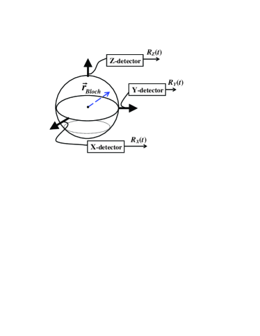
Figure 1: A qubit measured by three orthogonal detectors.

In this paper we study a recently suggested purification protocol based on monitoring of the qubit state via simultaneous continuous measurement of the three non-commuting qubit operators RuskovKorotkovMolmer $\hat{\sigma}_{x}$, $\hat{\sigma}_{y}$, $\hat{\sigma}_{z}$ (Fig.1). (A related protocol based on simultaneous measurement of these observables was first considered in Ref.WeiNazarov .) In contrast to the above purification protocols there is no need to perform Hamiltonian feedback. In this sense it is an “open loop” protocol, similar to the “random unitary control” purification protocols introduced in Ref. ComWisSco10 for spin-$j$ systems. Though operationally different, the two protocols can be shown to be equivalent in the special ($j=1/2$) case, which is another consequence of the isotropy of the qubit evolution discussed below.

Considering the rate of average purification under ideal measurements (with detector efficiency $\eta=1$) the purification speed-up is $4$, (this speed-up is implicit in the results of Ref. RuskovKorotkovMolmer ). Here the comparison is with a single measurement of the same strength with no feedback (the speed-up of $4/3$ quoted in Ref. ComWisSco10 comes from keeping the total measurement strength the same in the two protocols). However, we show here that by the alternate metric — the mean time $\langle T\rangle$ of first passage — the speed-up is only $2$. Both of these purification speed-ups can be understood via the isotropy of the qubit evolution RuskovKorotkovMolmer in the Bloch space that allows one to represent the three detectors by another equivalent detector triad, $\hat{\sigma}_{x^{\prime}}$, $\hat{\sigma}_{y^{\prime}}$, $\hat{\sigma}_{z^{\prime}}$, measuring at each time moment along the state and in the complementary directions.

We also study the purification dynamics for inefficient detectors, $\eta=1-\delta<1$. In the asymptotic high-purity limit ($\varepsilon,\delta\ll 1$) the increase $\Delta{\bar{T}}(\delta,\varepsilon)$ of the mean time of first passage $\langle T\rangle$ shows a scaling behavior (i.e. it depends only on the ratio ${\delta}/{\varepsilon}$) as seen from numerical calculations. The increase $\Delta{\bar{T}}({\delta}/{\varepsilon})$ is linear for relatively small inefficiency but grows exponentially, reaching $\sim\exp({\delta}/2{\varepsilon})$ for relatively large inefficiency.

II Further background: Single detector purification protocols

II.1 Qubit impurity from single-detector measurement

For a quantum-limited detector, in the limit of infinite detector bandwidth, the evolution of the state $\rho(t)$ of a quantum system due to weak continuous measurements of a variable $X$ can be described by the stochastic master equation (SME) WisemanMilburn-control :

$$d\rho=\frac{\Gamma_{0}}{2}\,dt\,{\cal D}[X]\,\rho+\sqrt{\frac{\Gamma_{0}}{2}}\,dW(t)\,{\cal H}[X]\,\rho.$$ (1)

Here ${\cal D}[A]\rho\equiv A\rho A^{{\dagger}}-\frac{1}{2}(A^{{\dagger}}A\rho+\rho A^{{\dagger}}A)$, ${\cal H}[A]\rho\equiv A\rho+\rho A^{{\dagger}}-\mbox{Tr}[(A^{{\dagger}}+A)\rho]\rho$, and $dW$ is the increment of a Wiener noise process. The internal Hamiltonian evolution of the system is either neglected (in case of a large measurement strength $\Gamma_{0}$), or eliminated (see, e.g. Ref. JordanKorotkov ). The measurement rate $\Gamma_{0}$ sets the rate at which information (about the final state) is extracted, and thus the rate at which the system is projected onto a single eigenstate of $X$ Korotkov-99-01 ; VanStoMab0605 (provided the spectrum of $X$ is non-degenerate). We will specialize on the measurement of a qubit and choose first $X=\hat{\sigma}_{z}$, although some results below are valid for a general $X$.

The measurement record in a small time interval $[t,t+dt)$ is given by

$$dR(t)=\langle X\rangle\,dt+dW(t)/\sqrt{2\Gamma_{0}},$$ (2)

where $\langle X\rangle=\mbox{Tr}[X\rho(t)]$, and $dW(t)$ is the same realization of the Wiener increment that appears in Eq. (1), thus providing explicit dependence of the state evolution on the specific measurement result. The evolution generated via Eq. (1) corresponds to infinitesimal measurement operators (see, e.g. Refs. WisemanMilburn-control ; JacobsSteck ; JordanKorotkov ). Since the same observable $X$ is measured at each time step, these operators commute, allowing one to integrate Eq. (1) exactly. Thus, for a finite time interval $[0,\tau)$ the final state will depend only on the time-averaged measurement record:

$$\mu(\tau)=\frac{1}{\tau}\int_{0}^{\tau}dt^{\prime}dR(t^{\prime}).$$ (3)

Introducing the measurement operator WisemanMilburn-control

$$M_{\mu,z}\equiv\left(\frac{\Gamma_{0}\tau}{\pi}\right)^{1/4}\exp{[-(\mu-\hat{\sigma}_{z})^{2}\frac{\Gamma_{0}\tau}{2}]}$$

one obtains, using the method of un-normalized density matrices (see, e.g. Refs. GoeGra94 ; Wis96 ; JacKni98 ; JacobsSteck ):

$$\rho(\tau,\mu)=\frac{M_{\mu,z}\rho(0)M_{\mu,z}^{{\dagger}}}{P(\mu)}.$$ (4)

Here the probability distribution for ${\mu}(\tau)$ is given by $P({\mu})=\mbox{Tr}[\rho M_{\mu,z}^{{\dagger}}M_{\mu,z}]$.

In the basis of the observable $X$, $\{|i\rangle\}$, the above result can be written as a quantum Bayesian filter Caves ; Korotkov-99-01 : the update of the diagonal density matrix elements $\rho_{ii}$ will look exactly as a classical Bayesian update of a “probability distribution”: $\rho_{ii}(\tau)=\rho_{ii}(0)P(\mu|i)/P(\mu)$, with Gaussian likelihoods $P(\mu|i)$; this was termed in Ref. Korotkov-99-01 the quantum-classical correspondence principle. The outcomes $\mu$ will be Gaussian distributed around the eigenvalues of $X$, $\{x_{i}\}$: $P(\mu|i)=\sqrt{\Gamma_{0}\tau/\pi}\exp[-(\mu-x_{i})^{2}\Gamma_{0}\tau]$ with variance $\mbox{Var}=1/2\Gamma_{0}\tau$, and expected outcome probability $P(\mu)=\sum_{i}\rho_{ii}P(\mu|i)$. The update of the non-diagonal matrix elements in (4) will be according to the rule: $\rho_{ij}(\tau)=\rho_{ij}(0)\sqrt{\rho_{ii}(\tau)\rho_{jj}(\tau)/\rho_{ii}(0)\rho_{jj}(0)}$ provided the measurement is preformed by a quantum-limited detector; this implies that a pure state will remain pure WisemanMilburn-control . From the above it is clear that the measurement time $\tau_{\rm meas}$ to distinguish approximately two eigenvalues, $x_{i},x_{j}$ is set by $\mbox{Var}|_{\tau_{\rm meas}}=(x_{i}-x_{j})^{2}/4$. For a qubit this gives $\tau_{\rm meas}=1/2\Gamma_{0}$ Korotkov-99-01 .

For further use we also write down the quantum state evolution in terms of the Bloch vector components of the state, $x=2\mbox{Re}\rho_{12}$, $y=2\mbox{Im}\rho_{12}$, $z=\rho_{11}-\rho_{22}$. From Eq. (1) for the measurement of $\hat{\sigma}_{z}$ it follows:

$$dz=(1-z^{2})\,\sqrt{2\Gamma_{0}}\,\,dW$$

$$dx=-\frac{\Gamma_{0}}{\eta}\,x-zx\,\sqrt{2\Gamma_{0}}\,\,dW$$

$$dy=-\frac{\Gamma_{0}}{\eta}\,y-zy\,\sqrt{2\Gamma_{0}}\,\,dW.$$ (5)

In these equations we also included the effect of detector non-ideality (inefficiency) $\eta$, leading to a pure dephasing : In the ensemble averaged equations (since Eqs.(5) are in the Itô form, averaging means just to drop the noise term, and corresponds to ignoring the detector results), $\Gamma_{0}$ is the decoherence rate due to an ideal detector of measurement rate $\Gamma_{0}$, and $\eta=\Gamma_{0}/(\Gamma_{0}+\gamma)\leq 1$ is the detector efficiency (ideality), defined as the ratio of $\Gamma_{0}$ to the total decoherence $\Gamma=\Gamma_{0}+\gamma$. For a single detector the simplest model to describe the extra decoherence $\gamma$ is to consider a second independent detector “in parallel” (i.e., measuring the same $\hat{\sigma}_{z}$ variable) by adding terms similar to Eq. (1) with $\Gamma_{0}$ replaced by $\gamma$, and subsequently averaging over that detector output. Thus, the density matrix available for an observer who takes into account only the results of the first detector will be described by Eqs.(5).

II.2 Single-detector purification protocols

We consider first purification protocols via single-detector measurement with an ideal (quantum-limited) detector.

II.2.1 Purification without feedback

For a single detector measurement without feedback, the state evolution in the detector basis is essentially classical, Eq. (4). That is, if the density matrix begins diagonal in the measurement basis (as it will be if it is a completely mixed state), it remains so and there is no way to distinguish $\{\rho_{11}(t),\rho_{22}(t)\}$ from a classical probability distribution Korotkov-99-01 ; RuskovKorotkovMizel . For continuous measurement one can consider the purity or entropy of the monitored state, and in this particular case the von Neumann entropy of the state coincides with the Shannon entropy (see, e.g. Refs. NielsenChuang ; Tribus61 ): $S_{\rm vN}=-\mbox{Tr}[\hat{\rho}\,\ln\hat{\rho}]=-\left(\rho_{11}\ln{\rho_{11}}+\rho_{22}\ln{\rho_{22}}\right)$. In what follows we will consider the so called linear entropy (see, e.g. FuschJacobs01 ), $s=1-\mbox{Tr}\hat{\rho}^{2}\equiv 1-p$ which is a monotonic function of $S_{\rm vN}$. Here $p\equiv\mbox{Tr}\hat{\rho}^{2}=\frac{(1+x^{2}+y^{2}+z^{2})}{2}$ is the purity expressed through the Bloch components of the state.

The corresponding equation for the purity (at $\eta=1$) follows from Eq. (5):

$$dp=2\Gamma_{0}\,\left[(1-p)(1-z^{2})\right]dt+2\sqrt{2\Gamma_{0}}\,z(1-p)\,dW.$$ (6)

Since purity $p$, like entropy, is invariant under unitary transformations, without loss of generality one can say that measurement “parallel to” (in the same basis as) the state corresponds to $x=y=0$ and

$$dp=\Gamma_{0}\,[1-z^{2}]^{2}dt+\sqrt{2\Gamma_{0}}\,z[1-z^{2}]\,dW.$$ (7)

so that the average change of purity is $\langle dp\rangle_{\parallel}=\Gamma_{0}\,(1-z^{2})^{2}dt$. We note that the same result holds for non-ideal measurement, $\eta<1$, since the detector’s non-ideality affects only the evolution of the non-diagonal density matrix elements; this means that a non-ideal detector will purify the state if the measurement is along the state. It is clear that $\Gamma_{0}$ plays the role of a maximal classical purification (information acquisition) rate that happen when $z=\rho_{11}-\rho_{22}=0$, i.e. when the two outcomes are equally likely (see, e.g., Ref. Tribus61 ). By approaching $z\rightarrow\pm 1$, $\langle dp\rangle_{\parallel}\rightarrow 0$ since “little information” remains to be extracted to clarify that collapse has happened pre-existing .

II.2.2 Jacobs feedback purification protocol

From the discussion above, it is intuitively clear how the Jacobs’ enhanced purification protocol works. Given the state $\rho(t)$, one should continuously adapt the measurement basis [or, equivalently, rotate the state to some $\rho^{\prime}(t)$] so that the detector would perform measurement in a complementary direction with respect to the eigenbasis of the rotated state (i.e., measuring perpendicular to the state, in the Bloch picture). In the detector basis the rotated state again possesses equally likely outcomes, with $\rho^{\prime}_{11}(t)=\rho^{\prime}_{22}(t)$. As expected classically Tribus61 , this procedure maximizes the average purification rate since $p=p^{\prime}$ under rotation, while $z\rightarrow z^{\prime}=0$ in Eq. (6). However, the possibility to perform coherent rotations of the density matrix is of course a quantum mechanical effect. The procedure also makes the purity evolution deterministic Jacobs , i.e. the noise term in Eq. (6) is zeroed so that

$$dp=2\Gamma_{0}\,(1-p)dt$$ (8)

and $\langle p\rangle=p$ under this protocol. From this one can evaluate the time $\tau_{\perp}$ when the average purity $\langle p\rangle$ reaches a given level $1-\varepsilon$:

$$\tau_{\perp}\simeq\frac{1}{2\Gamma_{0}}\int^{1-\varepsilon}\,\frac{dp}{1-p}\simeq\frac{1}{2\Gamma_{0}}\ln\varepsilon^{-1}.$$ (9)

It should be noted that an attempt to evaluate the analogous time $\tau_{\parallel}$ in the case of the classical measurement along the state, using $\langle dp\rangle_{\parallel}$ from Eq. (7), will lead to a wrong scaling of $\sim 1/\varepsilon$. The reason is that $\langle dp\rangle\neq d\langle{p}\rangle$ in general, and the evolving purity distribution ${\cal P}(p,t)$ is generally different from $\delta$-function WisemanRalph . The correct evaluation of $\tau_{\parallel}$ is to calculate the average purity $\langle p\rangle(t)$ by taking into account the exact solution, Eq. (4), of the stochastic evolution equations (1). In the high-purity limit this leads to Jacobs ; ComJac06 ; WisemanRalph ; JordanKorotkov

$$\tau_{\parallel}\simeq\frac{1}{\Gamma_{0}}\ln\varepsilon^{-1}$$ (10)

This is exactly twice as long as the time in Eq. (9), which establishes the speed-up of 2 for the Jacobs protocol. We note however, that, unlike the case of parallel measurement, the perpendicular measurement will not purify to a completely pure state if the measurement is inefficient, as will be explored in Sec. III.3. The reason is that the excess back-action in an inefficient perpendicular measurements results in decay in the coherences of the state.

II.2.3 Wiseman and Ralph purification protocol

Instead of considering the time $\tau$ at which the average purity $\langle p\rangle$ reaches a certain level $1-\varepsilon$, one can also consider the average time $\langle T\rangle$ for a system to attain that purity level, $p(T)=1-\varepsilon$ WisemanRalph ; WisBou08 ; ComWisJac08 . It was noted in Ref. WisemanRalph that in many circumstances the time $\langle T\rangle$ is a more useful quantity. The reason is that the time $T$ at which $p(T)=1-\varepsilon$, has a well-behaved statistics WisemanRalph , in contrast with $p(t)$ which has extremely long tails at relatively small values of $p$. That is, the averaged $\langle p\rangle$ is strongly influenced by the rare cases that are slow to purify. Because of this there is a substantial disagreement between $\tau$ and $\langle T\rangle$ for a qubit. It was shown in Ref. WisemanRalph , however, that good agreement is found between $\langle T\rangle$ and $T^{\rm log}{}$, defined as the time required for $\langle\ln[1-p(t)]\rangle$ to reach the certain level $\ln\varepsilon$. This is because taking the logarithm de-emphasizes the tails, and indeed for a qubit $\ln(1-p)$ has near-normal distribution WisemanRalph .

Therefore, we consider the stochastic equation for the logarithm of the linear entropy $s\equiv 1-p$. It follows from Eq. (6) that:

$$d\ln s=-2\Gamma_{0}\,\{2s+x^{2}+2z^{2}\}dt+2\sqrt{2\Gamma_{0}}\,z\,dW$$ (11)

(Here, without loss of generality we have put $y=0$, since a single $\hat{\sigma}_{z}$-measurement keeps the state of the qubit in a fixed meridional plane). In the Wiseman-Ralph feedback protocol WisemanRalph one keeps the monitored state along the detector $z$-axis (so $x^{2}=0$, while $z^{2}$ is maximized at $1-2s$). Thus, the single detector purification is maximized and in the high-purity limit, $s\approx 0$, we obtain $\frac{\langle d\ln s\rangle_{\parallel}}{dt}\simeq-4\Gamma_{0}$. Using this, the average time (of first passage) $\langle T\rangle$ is evaluated as $\langle T\rangle\simeq T^{\rm log}{}$ and in the high-purity limit, $\varepsilon\ll 1$

$$T^{\rm log}_{\parallel}=\frac{1}{4\Gamma_{0}}\ln{\varepsilon^{-1}},$$ (12)

which is half the size of $\tau_{\perp}$, and 4 times shorter than $\tau_{\parallel}$. In what follows we will use these results to understand the purification via three simultaneous complementary measurements without feedback.

III Continuous measurement of three complementary qubit variables

We consider continuous measurement of the qubit complementary observables $\hat{\sigma}_{x}$, $\hat{\sigma}_{y}$, and $\hat{\sigma}_{z}$ by three independent linear detectors (see Fig. 1). In principle, given a $\hat{\sigma}_{z}$-detector, the measurement of, say, $\hat{\sigma}_{x}$ can be implemented operationally by performing fast unitary rotation, $U_{x}(t)$, of the state towards the $x$-axis “at the beginning” of the measurement interval $dt$, then a continuous measurement with the $z$-detector and finally, a backwards transformation, $U_{x}^{-1}(t+dt)$ “at the end” , in any infinitesimal measurement time step $dt$, as discussed in Ref. ComWisSco10 . We also mention that a simultaneous measurement of the three observables is possible to implement, at least in principle, in a quantum optics setup RuskovMolmer-unpublished (e.g., using a single atom in an optical cavity field).

In the case of detectors measuring the qubit in the bases of non-commuting observables, it is impossible to use the quantum Bayes rule (4) for finite times because the measurement back-actions, $M_{\mu,x}$, $M_{\mu,y}$, $M_{\mu,z}$, do not commute with each other. The measurement back-actions commute only for small measurement time intervals $dt$ so that one should apply the POVM update in its differential form Eq. (1) and then sum up the contributions to the qubit evolution. For the case of mutually unbiased observables $\hat{\sigma}_{x}$, $\hat{\sigma}_{y}$, and $\hat{\sigma}_{z}$ it is convenient to use the Bloch vector components, $\boldsymbol{r}=(x,y,z)=\{\mbox{Tr}[\hat{\rho}\hat{\sigma}_{k}],k=x,y,z\}$ determined by the time-dependent qubit density matrix $\hat{\rho}$. From Eq. (5) for the influence due to $\hat{\sigma}_{z}$-measurement, the influences due to $\hat{\sigma}_{x}$ ($\hat{\sigma}_{y}$)-measurement can be obtained by cyclic replacements $z\rightarrow x\rightarrow y$, bearing in mind that the variables $x$($y$) should play the same role as $z$ in a $\hat{\sigma}_{z}$-measurement. In this way we obtain the following evolution equations in Itô form (see Ref. RuskovKorotkovMolmer ) that take into account the three measurement records $dR_{k}(t),k=x,y,z$ as in Eq. (2), and correspondingly introduce three independent Wiener processes, $dW_{i}\,dW_{k}=\delta_{ik}\,dt$:

$$dx=-(\Gamma_{y}+\Gamma_{z})\,x+(1-x^{2})\,\sqrt{2\Gamma_{0,x}}\,\,dW_{x}$$

$$\quad\qquad-x\,y\,\sqrt{2\Gamma_{0,y}}\,\,dW_{y}-x\,z\,\sqrt{2\Gamma_{0,z}}\,\,dW_{z}$$ (13)

$$dy=-(\Gamma_{z}+\Gamma_{x})\,y+(1-y^{2})\,\sqrt{2\Gamma_{0,y}}\,\,dW_{y}$$

$$\quad\qquad-y\,z\,\sqrt{2\Gamma_{0,z}}\,\,dW_{z}-x\,y\,\sqrt{2\Gamma_{0,x}}\,\,dW_{x}$$ (14)

$$dz=-(\Gamma_{x}+\Gamma_{y})\,z+(1-z^{2})\,\sqrt{2\Gamma_{0,z}}\,\,dW_{z}$$

$$\quad\qquad-x\,z\,\sqrt{2\Gamma_{0,x}}\,\,dW_{x}-y\,z\,\sqrt{2\Gamma_{0,y}}\,\,dW_{y}$$ (15)

Here $\Gamma_{k}\equiv\gamma_{k}+\Gamma_{0,k}$ are the total decoherence rates for each detector, including individual dephasings $\gamma_{k}$ and measurement rates $\Gamma_{0,k},k=x,y,z$. Note that a pure dephasing, say in the $x$-basis, causes the decay of the $z$- and $y$-components. Eqs. (14) and (15) are simply obtained by cyclic permutation of the variables in Eq. (13).

III.1 Qubit evolution with identical detectors

In what follows we consider the simplest (but still rich) case of three identical detectors: $\Gamma_{0,k}=\Gamma_{0}$ and $\gamma_{k}=\gamma\geq 0$. Then the qubit evolution (13)–(15) can be rewritten in a vector form as

$$d{\boldsymbol{r}}=-2\Gamma\,\boldsymbol{r}\,dt+\sqrt{2\Gamma_{0}}\,\,\left\{\boldsymbol{dW}(t)\,(1-r^{2})-\left[\boldsymbol{r}\times\left[\boldsymbol{r}\times\boldsymbol{dW}(t)\right]\right]\right\},$$ (16)

where $\boldsymbol{dW}(t)\equiv\{dW_{x},dW_{y},dW_{z}\}$ is the vector of Wiener increments corresponding to the vector of results $\boldsymbol{dR}=\{dR_{x},dR_{y},dR_{z}\}$, similar to Eq. (2). The evolution (16) is invariant under arbitrary rotations (see Fig. 2) of the coordinate system in Bloch space 3D-Gaussian (as is the ensemble averaged evolution: $\dot{\boldsymbol{r}}=-2\Gamma\,\boldsymbol{r}$). Hence while measurement of only a single observable $\hat{\sigma}_{k}$ “attracts” the qubit state to one of the corresponding eigenvectors, the simultaneous measurement of $\hat{\sigma}_{x}$, $\hat{\sigma}_{y}$, and $\hat{\sigma}_{z}$ leads to no preferable direction in the Bloch space. In Ref. RuskovKorotkovMolmer this isotropy of the qubit evolution was shown to lead to a locally isotropic Brownian diffusion of the direction of the Bloch vector. In particular, for pure states under ideal measurements, the point on the Bloch sphere diffuses isotropically Perrin with a diffusion coefficient $\Gamma_{0}$ RuskovKorotkovMolmer . The evolution isotropy was used then to construct simple quantum state estimations RuskovKorotkovMolmer . In what follows, we will use the qubit evolution isotropy to understand the qubit purification dynamics.

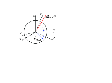
Figure 2: Bloch equations invariance under rotations for three complementary measurements with identical detectors. The evolution is determined by the relative orientation of the Bloch vector and the vector of results RuskovKorotkovMolmer .

III.2 Purification dynamics with three complementary measurements

Eq. (16) shows that the measurement term component along the radius is $\sqrt{2\Gamma_{0}}\,(\boldsymbol{dW}\cdot\boldsymbol{e_{r}})\,(1-r^{2})$ and vanishes on the sphere. The decreasing $r$-dependent coefficient suggests that $r=1$ is an attractor of the random evolution. Thus, the qubit state will purify in the ideal case ($\gamma=0$) for any realization of the measurement process.

To establish further the purification dynamics, we start with Eq. (16) and transform it to polar coordinates, $r$, $\theta$, $\phi$. The equation for the radius decouples from the other two and reads RuskovKorotkovMolmer :

$$dr=2\Gamma_{0}\,(1/r-r/\eta)dt+\sqrt{2\Gamma_{0}}(1-r^{2})\,dW_{r},$$ (17)

where $dW_{r}\equiv\boldsymbol{dW}\cdot\boldsymbol{e_{r}}$ is the projection of the noise vector onto the Bloch vector direction, $\boldsymbol{e_{r}}=(\sin\theta\cos\varphi,\sin\theta\sin\varphi,\cos\theta)$, and the normalization of the noise is $dW_{r}dW_{r}=dt$.

As seen from Eq. (17), if $r<\eta^{1/2}$, then on average $\dot{r}>0$, which means state purification for ideal measurements, $\eta=1$. Since the equation for $r$ is singular at the origin, it will be more convenient to consider further the dynamics of the purity $p=\mbox{Tr}\hat{\rho}^{2}=\frac{(1+r^{2})}{2}$. In this choice $1/2<p<1$, i.e., a totally mixed state corresponds to $p=1/2$. We find

$$dp=2\Gamma_{0}\,\{1-(2p-1)/{\eta}+2(1-p)^{2}\}dt+2\sqrt{2\Gamma_{0}}(1-p)\sqrt{2p-1}\,dW_{r}.$$ (18)

For an ideal measurement, $\eta=1$, and starting from a non-pure initial state, the qubit will purify ($p\rightarrow 1$) on a time scale of the order of $\tau_{\rm meas}\sim\Gamma_{0}^{-1}$. For a non-ideal measurement, $\eta<1$, purity will continue to fluctuate around a stationary average value, $\langle p\rangle_{\rm st}<1$.

III.2.1 Fokker-Planck equation for purity

To quantify the purity dynamics and asymptotic purity distribution we first consider the Fokker-Planck equation (FPE) corresponding to Eq. (18). Using the standard coefficients (see Ref. Gardiner ):

$$A(p)=2\Gamma_{0}\,[1-(2p-1)/{\eta}+2(1-p)^{2}]$$ (19)

$$B(p)=8\Gamma_{0}\,(2p-1)(1-p)^{2}$$ (20)

the FPE reads

$$\frac{\partial{\cal P}(p,t)}{\partial t}=-\frac{\partial}{\partial p}\left[A(p){\cal P}(p,t)\right]+\frac{1}{2}\,\frac{\partial^{2}}{\partial p^{2}}\,\left[B(p){\cal P}(p,t)\right],$$

and the initial distribution is taken to be ${\cal P}(p,0)=\delta(p-p_{0})$. At $t\gg\tau_{\rm meas}$ the purity reaches a stationary distribution RuskovKorotkovMolmer

$${\cal P}_{\rm st}(p,\eta)=N^{-1}\,\frac{\sqrt{2p-1}}{(1-p)^{3}}\,\exp{\left[-\frac{(2p-1)(1-\eta)}{2(1-p)\eta}\right]},$$ (21)

where $N$ is the normalization. For $\eta\rightarrow 1$, the stationary distribution ${\cal P}_{\rm st}(p,\eta)$ approaches the $\delta$-function at $p=1$.

The purification dynamics can be approximated using the ensemble-averaged purification rate Jacobs ; WisemanRalph obtained from the above Itô equation (18) for purity:

$$\langle dp\rangle=2\Gamma_{0}\,\langle 1-(2p-1)/{\eta}+2(1-p)^{2}\rangle\,dt.$$ (22)

Now consider a naive approach to integrating Eq. (22), in which we replace $p$ by $\langle p\rangle$ everywhere it appears on the right-hand-side:

$$\langle dp\rangle=2\Gamma_{0}\,\left[1-(2\langle p\rangle-1)/{\eta}+2(1-\langle p\rangle)^{2}\right]\,dt.$$ (23)

Contrary to the single-detector measurement, it can be shown, by numerically solving the FPE, that the evolution of the average purity $\langle p\rangle$ obtained from the naive Eq. (23) is very close to the true average $\langle p(t)\rangle_{\rm FP}=\int_{1/2}^{1}p\,{\cal P}(p,t)\,dp$, obtained from FPE. (The reasons for this difference will be discussed below.) Numerically, the approximation is best in the high purity limit ($\langle p\rangle=1-\langle s\rangle$, $\langle s\rangle\ll 1$) and for almost ideal detectors, $\eta\simeq 1$. In the high-purity limit we can discard terms of order $\langle s\rangle^{2}$ (i.e. the final term) so that Eq. (23) becomes a simple linear equation. For ideal measurements the time when the average purity reaches the level of $1-\varepsilon,\varepsilon\ll 1$ is thus

$$\tau_{\rm iso}\simeq\frac{1}{4\Gamma_{0}}\int^{1-\varepsilon}dp\frac{1}{1-p}=\frac{1}{4\Gamma_{0}}\ln{\varepsilon^{-1}},$$ (24)

which is four times shorter than the standard time $\tau_{\parallel}$ of classical measurements, Eq. (10). This means with three orthogonal measurements we obtain 4 times speed-up as compared to 2 times speed-up of the Jacobs (single measurement) purification protocol.

This result can be understood as follows. By the isotropy of the qubit evolution under three complementary measurements, in each time moment $t$ one can represent the measurements in the $x$, $y$, $z$ directions by measurements in an equivalent triple of directions $x^{\prime}$, $y^{\prime}$, $z^{\prime}$ (in the Bloch space, Fig. 2), chosen so that $z^{\prime}$ is parallel to the state (i.e., in the basis of $\hat{\sigma}_{z^{\prime}}$ the density matrix $\rho(t)$ is diagonal), while directions $x^{\prime}$, $y^{\prime}$ are perpendicular to the state; of course these chosen directions must change in time according to the evolution of the state, $\rho(t)$. The measurements in the $x^{\prime}$, $y^{\prime}$ directions in the time interval $[t,t+dt)$ are termed “good” measurements as they are precisely the unbiassed measurements of Jacobs that maximize the average purification rate, and the $z^{\prime}$-measurement along the state would be termed “bad” by obvious reason. This observation could be confirmed by rewriting Eq. (22) for $\eta=1$ in the following way:

$$\langle dp\rangle=2\Gamma_{0}\,\langle(1-p)+(1-p)+2(1-p)^{2}\rangle dt,$$ (25)

where the first two terms correspond to the deterministic change, $dp$, Eq. (8), and the last term coincides with the average change of $\langle dp\rangle_{\parallel}$ due to measurement along the state, Eq. (7). In the high purity limit, the last term is suppressed and the two “good” measurements contribute each a speed-up of 2 that amount to a total speed-up note1 of 4. Moreover, this makes clear why the naive approach (replacing $\langle p^{2}\rangle$ by $\langle p\rangle^{2}$) to calculating the mean purity works for the isotropic measurement: Jacob’s protocol gives deterministic growth of the purity, so that $\langle p^{2}\rangle=\langle p\rangle^{2}$. For isotropic measurement the purification in the mean is dominated by the perpendicular measurements, as just shown. Therefore the purification is approximately deterministic, and becomes more so the purer the state becomes. By contrast, with a single measurement and no control (the parallel measurement case), the purification is far from deterministic. In particular the long tail of low purities means it is impossible to obtain accurate results by replacing $\langle p^{2}\rangle$ by $\langle p\rangle^{2}$ WisemanRalph .

The “splitting” of the measurements into “good” and “bad” is also applicable when the goal of minimizing the mean time $\langle T\rangle$ is considered. As in the single-detector case WisemanRalph , we take the log-entropy evolution, $\ln{s},\,s=1-p$; similarly to that case $\ln s$ should have more symmetric distribution and therefore its average rate of change would correspond to the mean time of first passage (MTFP). Using Itô equation for three ideal detections, the average change of log-entropy in the high-purity limit ($s\to 0$) reads:

$$\langle d\ln s\rangle\simeq-8\Gamma_{0}\,dt=-(4+2+2)\Gamma_{0}\,dt,$$ (26)

i.e., the three detector measurements now “splits” into one “good” measurement ($z^{\prime}$), directed along the state, which gives the rate $4\Gamma_{0}$ as in Eq. (12) [Wiseman and Ralph protocol], and two “bad” measurements ($x^{\prime}$, $y^{\prime}$), directed perpendicular to the state, that give one-half of this rate each, see Eq. (9). Correspondingly, the mean time $\langle T\rangle\simeq T^{\rm log}$ for the average log-entropy $\langle\ln s\rangle$ to reach $\ln\varepsilon$ is given by

$$T^{\rm log}_{\rm iso}=\frac{1}{8\Gamma_{0}}\ln{\varepsilon^{-1}}.$$ (27)

This is two times shorter than the mean time for a single-detector no-control measurement, $T^{\rm log}_{\parallel}$, Eq. (12). Therefore, in comparison to the parallel single measurement case, three complementary measurements give a speed-up of 2 in terms of the mean time to attain a given purity. We will verify this result by explicitly calculating the MTFP, in the following subsection where we consider non-ideal detectors.

III.3 Purification dynamics for non-ideal detectors

It is now interesting to ask the question: Given non-ideal detectors with $\eta\equiv 1-\delta$, what level of purity, $p=1-\varepsilon$ can be reached and what time is needed? We now consider in detail this question, with emphasis on the high-purity and high-efficiency limit, when $\varepsilon\ll 1$ and $\delta\ll 1$. The answer to the above question will depend on the goal examined under purification.

III.3.1 The goal of having the average purity reach the level $(1-\varepsilon)$

Since the average purity $\langle p(t)\rangle_{\rm FP}$ described by the FPE is numerically close to that from the naive ensemble-average evolution Eq. (23), $\langle p(t)\rangle$ (see also Ref.RuskovKorotkovMolmer ), we will use the latter in our analysis. In particular, the stationary value $\langle p\rangle_{\rm st}$ is close to the true stationary value, obtained from the stationary distribution, Eq. (21), and reads:

$$\langle p\rangle_{\rm st}=1+\frac{1}{2}\left(\frac{1}{\eta}-\sqrt{\frac{1}{\eta^{2}}+\frac{2}{\eta}-2}\right).$$ (28)

In the high-ideality limit it gives $\langle p\rangle_{\rm st}\simeq 1-\frac{\delta}{2}$. Therefore, $\langle p\rangle$ can reach a purity level $(1-\varepsilon)$ only if

$$\varepsilon\geq\frac{\delta}{2}.$$ (29)

The time for $\langle p\rangle$ to reach $1-\varepsilon$ can be calculated from Eq. (23), and in the high-purity limit it gives:

$$\tau_{\rm iso}{(\delta,\varepsilon)}\simeq\frac{1}{4\Gamma_{0}}\left[\ln\frac{1}{2\varepsilon}-\ln\left(1-\frac{\delta}{2\varepsilon}\right)\right].$$ (30)

Here we note that the purification rate can be again understood by splitting into “good” and “bad” measurements. Indeed, the single detector average purification for $\eta<1$ can be calculated from Eq. (5):

$$\langle dp\rangle=2\Gamma_{0}\,\left\langle(1-p)(1-z^{2})+\frac{1}{2}\left(1-\frac{1}{\eta}\right)(2p-1-z^{2})\right\rangle dt,$$ (31)

and one can observe that $\langle dp\rangle$ is maximized for a measurement in perpendicular direction (${z}^{2}=0$) for not too small $\eta$ (e.g. even for a totally mixed state, $p=1/2$, this happens for $\eta>1/2$). Thus, the first term in Eq. (22) comes exactly from two “good” measurements (perpendicular to the state), $2\langle dp\rangle_{\perp}=1-(2p-1)/\eta$, while the second term comes from the “bad” measurement (parallel to the state) as in Eq. (7), and is suppressed in the high-purity limit. Therefore, the asymptotic result for $\tau_{\rm iso}{(\delta,\varepsilon)}$ comes entirely from the two good measurements, as in the ideal case. The time increase in Eq. (30) with respect to the ideal measurement, Eq. (24) is linear in the ratio $\delta/\varepsilon$ for $\delta\ll\varepsilon$ and diverges logarithmically to $\infty$ as the impurity level $\varepsilon$ approaches the bound, Eq. (29). To reach impurity level $\varepsilon<\frac{\delta}{2}$ is simply impossible.

III.3.2 The goal of having a certain mean time $\langle T\rangle$ at which the purity $p(T)$ reaches the level $(1-\varepsilon)$

We now proceed with the investigation of the mean time $\langle T\rangle$ for the purity to reach $p(T)=1-\varepsilon$ for three complementary non-ideal measurements. Following Ref. WisemanRalph we write the Itô equation for the log-entropy:

$$d\ln s\mid_{\rm iso}=-2\Gamma_{0}\,\left\{2-2s+\frac{2}{\eta}+\left(1-\frac{1}{\eta}\right)\frac{1}{s}\right\}dt+2\sqrt{2\Gamma_{0}}\sqrt{1-2s}\,dW_{r}.$$ (32)

Similar to the ideal case, the average change of log-entropy can be represented as a sum of the measurement along the state and two measurements perpendicular to the state. Indeed, the change $d\ln s$ for a single non-ideal detector can be written as:

$$d\ln s=-2\Gamma_{0}\,\left\{2s+x^{2}+2z^{2}+\left(1-\frac{1}{\eta}\right)\frac{x^{2}}{2s}\right\}dt+2\sqrt{2\Gamma_{0}}z\,dW.$$ (33)

We note that for given entropy $s=1-p$, the average change $\langle d\ln s\rangle$ is maximized again for $x^{2}=0$ and $z^{2}=1-2s$, and it coincides with the ideal case: $\langle d\ln s\rangle_{\parallel}=-2\Gamma_{0}dt\,\{2-2s\}$, see Eq. (12). On the other hand the change due to measurement in the complementary directions ($z=0$) is deterministic and read: $\langle d\ln s\rangle_{\perp}=d\ln s_{\perp}=-2\Gamma_{0}dt\,[\frac{1}{\eta}+(1-\frac{1}{\eta})/{2s}]$, so that $\langle d\ln s\rangle\mid_{\rm iso}=\langle d\ln s\rangle_{\parallel}+2\,\langle d\ln s\rangle_{\perp}$. By considering highly ideal detectors, $\eta\approx 1$, so that the last, singular, term in $d\ln s_{\perp}$ can be neglected, one can reproduce the mean time $\langle T\rangle$ by integration of the equation for $\langle d\ln s\rangle\mid_{\rm iso}$. However, in the high-purity limit this is not possible: naive integration of log-entropy, with the singular term, $\propto(1-\frac{1}{\eta})/{s}$, included, will lead to a wrong result. Since in the high-purity limit $\delta\ll 1$, $\varepsilon\ll 1$, this term is of the order of $\frac{\delta}{\varepsilon}$, it is clear that the time of reaching a certain purity level will be essentially affected when $\frac{\delta}{\varepsilon}\gtrsim 1$.

In what follows, we investigate the exact solution for the MTFP in case of inefficient detectors. We consider an initially completely mixed state, and denote the MTFP as $\bar{T}(\delta,\varepsilon)$. The FPE constructed above, based on the stochastic Itô Eq. (18) is used, where in the high-purity limit, we approximate the coefficient, Eq. (20), as: $B(p)\simeq B_{\rm HP}(p)=8\Gamma_{0}\,(1-p)^{2}$, while keeping $A(p)$ unchanged. The MTFP solution for one reflective boundary (at $p=1/2$) and one absorptive (at $p=1-\varepsilon$) is written as (see, e.g. Ref. Gardiner )

$${\bar{T}}(\delta,\varepsilon)=2\int_{p_{0}}^{1-\varepsilon}\frac{dy}{\psi_{\rm HP}(y,1-\delta)}\int_{1/2}^{y}dz\frac{\psi_{\rm HP}(z,1-\delta)}{B_{\rm HP}(z)},$$ (34)

where $p_{0}$ is the initial purity as before; in what follows we consider only $p_{0}=1/2$. The function that enters the solution is $\psi_{\rm HP}(x)=\exp{\int_{1/2}^{x}\,dx^{\prime}\frac{2A(x^{\prime})}{B_{\rm HP}(x^{\prime})}}$ and in our case one obtains

$$\psi_{\rm HP}(x,1-\delta)=\frac{\exp{(x-\frac{1}{2})\,f_{1-\delta}(x)}}{[2(1-x)]^{\frac{1}{(1-\delta)}}},$$ (35)

where we denoted $f_{1-\delta}(x)\equiv 1-\frac{\delta}{(1-x)(1-\delta)}$.

For ideal measurements, $\delta=0$, one can integrate Eq. (34) to obtain analytically the result:

$${\bar{T}}(0,\varepsilon)\approx\frac{1}{8\Gamma_{0}}\left(\ln{\varepsilon^{-1}}-1.35\right),$$ (36)

in agreement actual-B with the straightforward integration of the ensemble-averaged log-entropy equation, [see Eqs.(26) and (27) above]. For $\delta>0$ analytical integration is not as obvious: naive expansion of the integrand in series in $\delta$ leads to a sum of contributions with increasing singularities. We present instead numerical calculations that show the scaling behavior in the high-purity limit.

The main observation is that in the high-purity limit the time of purification can be represented as

$${\bar{T}}(\delta,\varepsilon)\simeq{\bar{T}}(0,\varepsilon)+\Delta{\bar{T}}\left(\frac{\delta}{\varepsilon}\right).$$ (37)

That is, the time increase $\Delta{\bar{T}}$ depends only on the ratio $a\equiv\frac{\delta}{\varepsilon}$. It can be shown that for $a\ll 1$, $\Delta{\bar{T}}\left(a\right)\simeq(1/8\Gamma_{0})\frac{a}{6}$, while for $a\gg 1$, $\Delta{\bar{T}}\left(a\right)\approx(1/8\Gamma_{0})\exp{[C_{1}(a)\,a]}$, with $0.25\lesssim C_{1}(a)<0.5$, approaching 0.5 for large $a$.

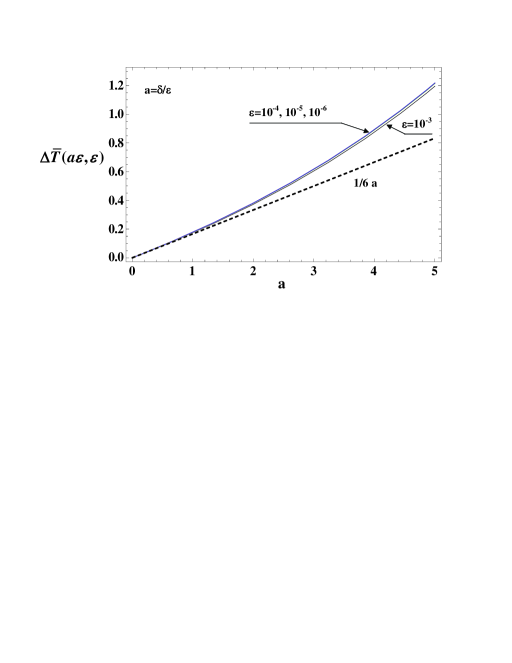
Figure 3: The mean time increase, $\Delta\bar{T}(a\varepsilon,\varepsilon)$, for small $a<5$, and $\varepsilon\ll 1$; Scaling is established for $\varepsilon\lesssim 10^{-4}$.

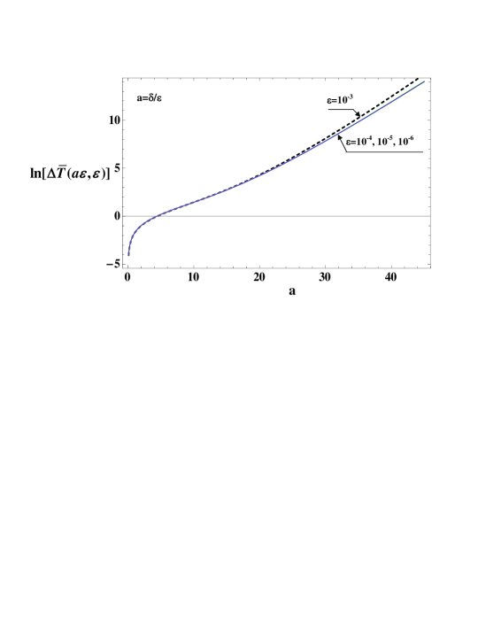
Figure 4: The approximate linear growth of the logarithm of mean time increase, $\ln[\Delta\bar{T}(a\varepsilon,\varepsilon)]\approx C_{1}a$, for large $a\gg 1$, and $\varepsilon\ll 1$; Scaling is for $\varepsilon\lesssim 10^{-4}$.

On Figs. 3 and 4 we present evidence of scaling. Fig. 3 shows $\Delta\bar{T}(a)={\bar{T}}(a\varepsilon,\varepsilon)-{\bar{T}}(0,\varepsilon)$ at fixed $\varepsilon$ and for $a<5$. The curve for $\varepsilon=10^{-3}$ is close to the curves for $\varepsilon=10^{-4},10^{-5},10^{-6}$ that practically coincide on the figure; the slope at $a=0$ is $1/6$. Fig. 4 shows the scaling for large $a$. The $\ln[\Delta\bar{T}(a)]$, eventually approaches a single curve for $\varepsilon\ll 1$. For $a\gtrsim 20$ it looks like a linear growth, i.e. $\ln[\Delta\bar{T}(a)]\approx C_{1}a$. More precisely, by numerical calculation of the derivative $d\ln[\Delta\bar{T}(a)]/da$ (not shown) one can see that it is not a constant but varies somewhat as discussed above. For small enough $\varepsilon$ ($a>2000$), $C_{1}$ approaches $1/2$. Thus, the numerical calculations support Eq. (37).

IV Conclusion

In this paper we investigate in detail a recently proposed quantum state purification protocol based on simultaneous continuous measurement of the three complementary observables for a qubit: $\hat{\sigma}_{x}$, $\hat{\sigma}_{y}$, $\hat{\sigma}_{z}$. Contrary to analogous single-detector purification protocols, that are based on complementarity Jacobs ; WisemanRalph ; ComJac06 ; ComWis11 , and which require feedback control, here there is no need of introducing quantum feedback. However, interestingly enough, the purification dynamics of our protocol can be understood via the above mentioned protocols, using the established isotropy of the qubit evolution under three complementary measurements by identical detectors RuskovKorotkovMolmer .

For ideal (i.e. quantum-limited, or efficient) measurements, our main results are the observation of different factors for the speed-up (relative to a single measurement in the eigenbasis of the qubit state), of 4 and 2, depending on how the purification speed is quantified. In the first case it is in terms of the time when the average system purity, $\langle p\rangle$, reaches certain purity level $1-\varepsilon$; in the second case it is in terms of the mean time $\langle T\rangle$ at which the purity $p(T)$ first attains the set level of $1-\varepsilon$. Both of these speed-ups can be understood via the possibility to “split” the three detector measurement at each measurement time step into three equivalent measurements — one parallel to the state (in the Bloch sphere sense) and the remaining two perpendicular to the state — which is one of the consequences of isotropy of the qubit evolution in the Bloch space. For the first measure of purification time these correspond to one “bad” and two “good” measurements (giving speed-up contributions of $0$ and $2+2$ respectively, totalling 4). For the second measure, they correspond to one “good” and two ”bad” measurements (giving speed-up contributions of $1$ and $1/2+1/2$ respectively, totalling 2).

For a measurement with non-ideal detectors, the dynamics remains isotropic in the Bloch space. Moreover, the classification to “good” and “bad” measurements remains the same, as long as the detector inefficiency $\delta$ is not greater than $1/2$. The inefficiency causes an increase in the purification times, that scales as a function of the ratio of inefficiency over impurity, $\delta/\varepsilon$, in the high-purity and high-efficiency limit, $\delta\ll 1$, $\varepsilon\ll 1$. Here, the first speed-up quantification, stated in terms of attaining a certain average purity, is simply impossible if $\varepsilon<\frac{\delta}{2}$, and the time required diverges as $\varepsilon$ approaches this limit from above. On the other hand, the second quantification, stated in terms of the mean time for individual (stochastically evolving) systems to attain this purity, always gives an answer. However we show that the mean time increases exponentially: $\propto\exp{[0.5\,\delta/\varepsilon]}$ for very large $\delta/\varepsilon$ ratio. Still, for moderate $\delta/\varepsilon\gtrsim 1$ the mean time is not too much greater than the ideal case estimation.

- (1) M. A. Nielsen and I. L. Chuang, Quantum Computation and Quantum Information (Cambridge University Press, Cambridge, UK, 2000).
- (2) H. M. Wiseman and G. J. Milburn, Quantum Measurement and Control (Cambridge University Press, Cambridge, UK, 2010).
- (3) H. M. Wiseman and G. J. Milburn, Phys. Rev. Lett. 70, 548 (1993); Phys. Rev. A 49, 1350 (1994).
- (4) H. F. Hofmann, G. Mahler, and O. Hess, Phys. Rev. A 57, 4877 (1998); H. M. Wiseman and S. Mancini and J. Wang, Phys. Rev. A 66, 013807 (2002).
- (5) R. Ruskov and A. N. Korotkov, Phys. Rev. B 66, 041401(R) (2002); Q. Zhang, R. Ruskov, and A. N. Korotkov, Phys. Rev. B 72, 245322 (2005); A. N. Korotkov, Phys. Rev. B 71, 201305(R) (2005).
- (6) R. Ruskov and A. N. Korotkov, Phys. Rev. B 67, 241305(R) (2003); W. Mao, D. V. Averin, R. Ruskov, and A. N. Korotkov, Phys. Rev. Lett. 93, 056803 (2004).
- (7) C. Ahn, A. C. Doherty, and A. J. Landahl, Phys. Rev. A, 65, 042301 (2002); C. Ahn , H. M. Wiseman, and G. J. Milburn, ibid. 67, 052310 (2003); M. Sarovar, C. Ahn, K. Jacobs, and G. J. Milburn, ibid. 69, 052324 (2004).
- (8) K. Jacobs, Phys. Rev. A 67, 030301(R) (2003)
- (9) J. Combes and K. Jacobs, Phys. Rev. Lett. 96, 010504 (2006).
- (10) H. M. Wiseman and J. F. Ralph, New J. of Phys. 8, 90 (2006).
- (11) A. N. Jordan and A. N. Korotkov, Phys. Rev. B 74, 085307 (2006).
- (12) J. Combes, H. M. Wiseman and K. Jacobs, Phys. Rev. Lett. 100, 160503 (2008).
- (13) H. M. Wiseman and L. Bouten, Quantum Information Processing 7, 71 (2008).
- (14) V. P. Belavkin and A. Negretti and K. Mølmer, Phys. Rev. A, 79, 022123 (2009).
- (15) R. Ruskov, A.N. Korotkov, and K. Mølmer, Phys. Rev. Lett. 105, 100506 (2010).
- (16) H.-D. Wei and Yu. V. Nazarov, Phys. Rev. B 78, 045308 (2008).
- (17) J. Combes, H. M. Wiseman, and A.J. Scott, Phys. Rev. A 81, 020301(R) (2010).
- (18) A. N. Korotkov, Phys. Rev. B 63, 115403 (2001); Phys. Rev. B 60, 5737 (1999).
- (19) R. van Handel, J. K. Stockton and H. Mabuchi, IEEE Trans. on Automatic Control 50, 768 (2005).
- (20) P. Goetsch and R. Graham, Phys. Rev. A. 50, 5242 (1994).
- (21) H. M. Wiseman, J. Opt. B: Quantum and Semiclassical Opt. 8 , 205 (1996).
- (22) K. Jacobs and P. L. Knight, Phys. Rev. A. 57, 2301 (1998).
- (23) K. Jacobs and D. Steck, Contemp. Phys. 47, 279 (2006).
- (24) C. M. Caves, Phys. Rev. D 33, 1643 (1986).
- (25) R. Ruskov, A. N. Korotkov, and A. Mizel, Phys. Rev. Lett. 96, 200404 (2006).
- (26) C. A. Fuchs and K. Jacobs, Phys. Rev. A 63, 062305 (2001).
- (27) R. Ruskov and K. Mølmer, unpublished.
- (28) M. Tribus, Thermostatics and Thermodynamics: An Introduction to Energy, Information and States of Matter, with Engineering Applications, (Van Nostrand, 1961), p. 64.
- (29) An important difference is that a classical Bayesian inference reveals a pre-existing system state (e.g. a “true” probability distribution), while quantum evolution, Eqs. (1), (2), is about the (final) quantum state available to an experimentalist.
- (30) In the rotated frame of Fig. 2, the joint distribution of Wiener noises is still the same Gaussian distribution, since the measurements commute for small times.
- (31) F. Perrin, C.R. Acad. Sci., Paris, 181, 514 (1925).
- (32) C. W. Gardiner, Handbook of Stochastic methods (Springer, Berlin, 1983).
- (33) Using the actual FPE coefficient , Eq. (20), numerical integration of Eq. (34) gives for the MTFP, , which differs negligibly from Eq.(27) for large .
- (34) J. Combes and H. M. Wiseman, Phys. Rev. X 1, 011012, (2011).
- (35) In the absence of the two “good” measurements the noise term must be taken into account to calculate the average purity .