Cavity approach to sphere packing in Hamming space

A. Ramezanpour Physics Department and Center for Computational Sciences, Politecnico di Torino, Corso Duca degli Abruzzi 24, 10129 Torino, Italy    R. Zecchina Physics Department and Center for Computational Sciences, Politecnico di Torino, Corso Duca degli Abruzzi 24, 10129 Torino, Italy Human Genetics Foundation, Torino, via Nizza 52, 10126 Torino, Italy Collegio Carlo Alberto, Via Real Collegio 30, 10024 Moncalieri, Italy
Abstract

In this paper we study the hard sphere packing problem in the Hamming space by the cavity method. We show that both the replica symmetric and the replica symmetry breaking approximations give maximum rates of packing that are asymptotically the same as the lower bound of Gilbert and Varshamov. Consistently with known numerical results, the replica symmetric equations also suggest a crystalline solution, where for even diameters the spheres are more likely to be found in one of the subspaces (even or odd) of the Hamming space. These crystalline packings can be generated by a recursive algorithm which finds maximum packings in an ultra-metric space. Finally, we design a message passing algorithm based on the cavity equations to find dense packings of hard spheres. Known maximum packings are reproduced efficiently in non trivial ranges of dimensions and number of spheres.

I Introduction

The problem of packing rigid objects, and spheres in particular, is a fundamental problem which appears across disciplines TS-rmp-2010 ; PZ-rmp-2010 . In general, the objects could have arbitrary shapes and the ambient space can be an abstract space ΛΛ\Lambda. Given the space and the objects, the main question is that of finding the densest packings.

In coding theory one is interested in finding an optimal representation of N𝑁N symbols in binary strings of length n𝑛n, that is Λ={0,1}nΛsuperscript01𝑛\Lambda=\{0,1\}^{n} is the Hamming space of dimension n𝑛n. This optimal coding contains as many as possible symbols and ensures that after transmitting through a noisy channel, which at most flips d12𝑑12\frac{d-1}{2} variables, one can recover the original messages. The ratio between the characteristic length of the symbols lclog2Nsubscript𝑙𝑐subscript2𝑁l_{c}\equiv\log_{2}N and length of the transmitted strings n𝑛n defines the rate of coding (or packing). The maximum rate of coding is denoted by R𝑅R. Indeed people are interested to know the asymptotic form of R𝑅R when n,d𝑛𝑑n,d\rightarrow\infty and δd/n𝛿𝑑𝑛\delta\equiv d/n remains constant. So far there is a considerable difference between the best lower and upper bounds for R𝑅R H-bell-1950 ; G-bell-1952 ; V-akad-1957 ; MRRW-inform-1977 ; PL-inform-1998 ; BJ-codes-2001 ; S-jcomb-2001 ; JV-inform-2004 . This means that for large n𝑛n the best lower and upper bounds for the number of symbols differ by a factor of order 2nsuperscript2𝑛2^{n}.

Physically, one can consider the set of symbols as a system of identical particles in the Hamming space of dimension n𝑛n, interacting by a hard core potential of range d𝑑d PS-jstatphys-1999 ; PZ-jstatphys-2006 . The aim is then to study the physical states of different densities. Clearly for small densities the system is in the liquid phase respecting the translational symmetry. In this case it is easy to calculate, for example, the entropy. At higher densities the liquid entropy becomes incorrect (negative) signaling the onset of other stable phases, either crystalline or glassy PZ-jchemphys-2005 ; PZ-jstatmech-2006 .

In this study we formulate the packing problem as a constraint satisfaction problem. We consider N𝑁N variables (the physical particles or the strings of symbols) which take values in ΛΛ\Lambda and for each pair of the variables we consider a constraint that forbids overlapping assignments of the two variables. A packing is thus an assignment of the variables that satisfies all the constraints. This representation differs substantially with the so called lattice gas models where binary variables (representing occupied or empty positions) are defined one each point of the space ΛΛ\Lambda.

The cavity method provides analytical and numerical tools which can be extremely useful in solving optimization problems (or constraint satisfaction problems) over random structures MP-epjb-2001 ; MPZ-science-2002 ; MZ-pre-2002 ; MP-jstatphys-2003 ; MPV-1987 . In certain cases it is known to provide sampling results which cannot be obtained by Monte Carlo Markov chains in subexponential times [e.g. optimization problems in the one-step replica symmetry breaking (1RSB) phase]. As an optimization tool it often outperforms linear programming methods PNAS-nosotros-2011 . The development of such algorithm is, however, by no means obvious due to the choice of the representation of the problem and to the need of writing the cavity equations in an algorithmically efficient form.

As we shall discuss in this paper, insights from the application of the cavity method will turn out to be also useful in the study of the type of packing problems we are interested in.

In this paper we study the cavity equations for the packing problem in the replica symmetric (RS) and in the one-step replica symmetry breaking (1RSB) approximations MPV-1987 . These equations are called belief propagation (BP) and survey propagation (SP) equations, respectively MZ-pre-2002 ; BMZ-rsa-2005 . In the RS approximation, besides a liquid solution we find a crystalline phase where with higher probability spheres are found in one of the sublattices (even or odd) of the Hamming space. This phase has already been observed in Monte Carlo simulations of Ref. PZ-jstatmech-2006 . Both the liquid and crystalline solutions predict a maximum rate of packing that behaves asymptotically like the best known lower bound JV-inform-2004 . The same result has been obtained in Ref. PZ-jstatphys-2006 where the liquid entropy is computed in the hypernetted chain approximation. To discuss the exactness of the cavity free entropy we also consider some interpolation techniques which connect the cavity free entropy to the true entropy of the system G-commath-2003 ; FL-jstatphys-2003 ; FLT-jstatphys-2003 .

In the 1RSB case, we provide an approximate solution of the SP equations to calculate the configurational entropy, defined as the (log of) the number of pure states or clusters in the solution space. This quantity acquires a nonzero value at a clustering transition where the liquid entropy is still positive. The maximum rate of packing that is achievable still coincides with the one obtained in the RS approximation.

Finally we design a message passing algorithm based on the BP equations which allows us to find dense packings in not too large dimensions. These packings are typically hard to find by other simple methods like Monte Carlo based algorithms. Unfortunately the computation time and memory increase exponentially with the space dimension n𝑛n, making larger dimensions very difficult to explore. To partially overcome this problem we introduce an approximate update rule for the message passing algorithm which is restricted to a subspace and makes the computation more efficient. This improvement, together with the distributive nature of the algorithm, could help to run the algorithm in larger dimensions. We also discuss another iterative algorithm that, given a packing configuration of spheres with diameter d𝑑d, finds another packing for larger diameter d+1𝑑1d+1 by increasing the space dimension n𝑛n. This is a polynomial time algorithm generating maximum packings in an ultrametric space. When applied to our problem, we find crystalline packings predicted by the RS cavity equations for even sphere diameters.

The structure of the paper is as follows. In Sec. II we define the problem more precisely and give a summary of known results. In Secs. III and IV we present the BP and SP equations and study their consequences for the hard sphere packing problem. In Sec. V we study the packing algorithms and Sec. VI is devoted to extension to the q𝑞q-ary Hamming spaces. Finally the concluding remarks are given in Sec. VII. In the first two appendixes we give the details of calculations for checking the stability of the BP solutions and deriving the SP equations. The interpolation methods and some of their properties are presented in Appendix C.

II Definitions and known results

Consider N𝑁N hard spheres of diameter d𝑑d indexed by i=1,,N𝑖1𝑁i=1,\ldots,N and a Hamming space of dimension n𝑛n. The set of points in this space are denoted by Λ={0,1}nΛsuperscript01𝑛\Lambda=\{0,1\}^{n} with size |Λ|=2nΛsuperscript2𝑛|\Lambda|=2^{n}. We index the points in this space by σ𝜎\sigma. A point can be represented by a binary vector of n𝑛n elements {0,1}absent01\in\{0,1\}. The Hamming space can be partitioned into two subspaces: even and odd. Points in the even subspace have an even number of 111’s (even parity) and those in the odd subspace have an odd number of 111’s (odd parity). The Hamming distance D(σ,σ)𝐷𝜎superscript𝜎D(\sigma,\sigma^{\prime}) between two points σ𝜎\sigma and σsuperscript𝜎\sigma^{\prime} is equal to the number of different elements in the binary representation of the two points. For each point σ𝜎\sigma we define the set Vd(σ)subscript𝑉𝑑𝜎V_{d}(\sigma) as

Vd(σ){σ|D(σ,σ)<d},Vd|Vd(σ)|=l=0d1(nl).formulae-sequencesubscript𝑉𝑑𝜎conditional-setsuperscript𝜎𝐷𝜎superscript𝜎𝑑subscript𝑉𝑑subscript𝑉𝑑𝜎superscriptsubscript𝑙0𝑑1𝑛𝑙V_{d}(\sigma)\equiv\{\sigma^{\prime}|D(\sigma,\sigma^{\prime})<d\},\hskip 28.45274ptV_{d}\equiv|V_{d}(\sigma)|=\sum_{l=0}^{d-1}\left(\begin{array}[]{c}n\\ l\end{array}\right). (1)

The aim is to find a non-overlapping configuration of spheres such that D(σi,σj)d𝐷subscript𝜎𝑖subscript𝜎𝑗𝑑D(\sigma_{i},\sigma_{j})\geq d, for any two spheres i𝑖i and j𝑗j. The above problem is a constraint satisfaction problem with N(N1)/2𝑁𝑁12N(N-1)/2 constraints to satisfy. We index these constraints by (ij)𝑖𝑗(ij). A configuration σ¯{σi|i=1,,N}¯𝜎conditional-setsubscript𝜎𝑖𝑖1𝑁\underline{\sigma}\equiv\{\sigma_{i}|i=1,\ldots,N\} that satisfies all the constraints is called a solution of the problem. The partition function Z𝑍Z counts the number of such solutions,

Z=σ¯i<jIij(σi,σj),𝑍subscript¯𝜎subscriptproduct𝑖𝑗subscript𝐼𝑖𝑗subscript𝜎𝑖subscript𝜎𝑗Z=\sum_{\underline{\sigma}}\prod_{i<j}I_{ij}(\sigma_{i},\sigma_{j}), (2)

where Iij(σi,σj)subscript𝐼𝑖𝑗subscript𝜎𝑖subscript𝜎𝑗I_{ij}(\sigma_{i},\sigma_{j}) is an indicator function for constraint (ij)𝑖𝑗(ij); it is 111 if D(σi,σj)d𝐷subscript𝜎𝑖subscript𝜎𝑗𝑑D(\sigma_{i},\sigma_{j})\geq d and 00 otherwise. The maximum rate of packing is defined as

Rlimn,d1nlog2(Nmax),𝑅subscript𝑛𝑑1𝑛subscript2subscript𝑁𝑚𝑎𝑥R\equiv\lim_{n,d\rightarrow\infty}\frac{1}{n}\log_{2}(N_{max}), (3)

with δ=d/n=const𝛿𝑑𝑛const\delta=d/n=\mathrm{const} and Nmaxsubscript𝑁𝑚𝑎𝑥N_{max} is the maximum number of spheres such that Z>0𝑍0Z>0.

Let us here mention some known lower and upper bounds for R𝑅R. The Gilbert and Varshamov (GV) lower bound G-bell-1952 ; V-akad-1957 states that

Nmax2nVd,subscript𝑁𝑚𝑎𝑥superscript2𝑛subscript𝑉𝑑N_{max}\geq\frac{2^{n}}{V_{d}}, (4)

resulting in the following lower bound for the maximum rate of packing

RRGV1H(δ),𝑅superscript𝑅𝐺𝑉1𝐻𝛿R\geq R^{GV}\equiv 1-H(\delta), (5)

where

H(δ)δlog2δ(1δ)log2(1δ).𝐻𝛿𝛿subscript2𝛿1𝛿subscript21𝛿H(\delta)\equiv-\delta\log_{2}\delta-(1-\delta)\log_{2}(1-\delta). (6)

Notice that 1H(δ)1𝐻𝛿1-H(\delta) is also the Shannon rate for a binary symmetric channel with error probability δ𝛿\delta. A better lower bound is obtained with graph theoretical methods JV-inform-2004 and gives

RRJV1H(δ)+log2[cnH(δ)]n,𝑅superscript𝑅𝐽𝑉1𝐻𝛿subscript2𝑐𝑛𝐻𝛿𝑛R\geq R^{JV}\equiv 1-H(\delta)+\frac{\log_{2}[cnH(\delta)]}{n}, (7)

where c𝑐c is a constant. As far as we know, this is the best lower bound reported for the maximum rate of packing. However, it still behaves asymptotically like RGVsuperscript𝑅𝐺𝑉R^{GV}. The authors in Ref. PZ-jstatphys-2006 use the liquid entropy of the system of hard spheres to find a maximum rate of packing that is very close to the above lower bound

RPZ1H(δ)+log2[(2ln2)nH(δ)]n.superscript𝑅𝑃𝑍1𝐻𝛿subscript222𝑛𝐻𝛿𝑛R^{PZ}\equiv 1-H(\delta)+\frac{\log_{2}[(2\ln 2)nH(\delta)]}{n}. (8)
Refer to caption
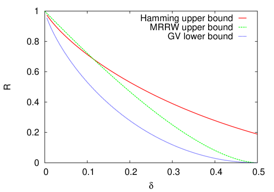
Figure 1: Comparing the known lower and upper bounds for the maximum rate of packing R𝑅R.

On the other side, we have the Hamming upper bound H-bell-1950

Nmax2nVd2,subscript𝑁𝑚𝑎𝑥superscript2𝑛subscript𝑉𝑑2N_{max}\leq\frac{2^{n}}{V_{\frac{d}{2}}}, (9)

resulting in

RRH1H(δ2),𝑅superscript𝑅𝐻1𝐻𝛿2R\leq R^{H}\equiv 1-H\left(\frac{\delta}{2}\right), (10)

The best upper bound for R𝑅R is obtained by the linear programming methods MRRW-inform-1977 . An overestimate of this linear programming bound is

RRMRRWH(12δ(1δ)).𝑅superscript𝑅𝑀𝑅𝑅𝑊𝐻12𝛿1𝛿R\leq R^{MRRW}\equiv H\left(\frac{1}{2}-\sqrt{\delta(1-\delta)}\right). (11)

In Fig. 1 we have compared the above bounds to show the large gap between the best lower and upper bounds.

III Replica symmetric solutions: BP equations

The basic objects in the cavity method are the cavity marginals or messages passed along the edges of the interaction graph MP-epjb-2001 ; MZ-pre-2002 ; MP-jstatphys-2003 . In our problem the messages are 2nsuperscript2𝑛2^{n}-component vectors with elements {0,1}absent01\in\{0,1\}. There are two kinds of messages: (i) The cavity bias 𝐮ijsubscript𝐮𝑖𝑗\mathbf{u}_{i\rightarrow j} represents the warning that variable i𝑖i sends to j𝑗j; uijσ=1(0)superscriptsubscript𝑢𝑖𝑗𝜎10u_{i\rightarrow j}^{\sigma}=1(0) says that point σΛ𝜎Λ\sigma\in\Lambda is (not) forbidden by i𝑖i for variable j𝑗j. (ii) The cavity field 𝐡ijsubscript𝐡𝑖𝑗\mathbf{h}_{i\rightarrow j} is sum of warnings that i𝑖i receives in absence of j𝑗j; hijσsuperscriptsubscript𝑖𝑗𝜎h_{i\rightarrow j}^{\sigma} gives the number unsatisfied constraints, in the absence of j𝑗j, if variable i𝑖i takes state σ𝜎\sigma. The cavity biases are

𝐮ij{𝐞σ|σΛ},eσσ={1,if σVd(σ);0,otherwise.formulae-sequencesubscript𝐮𝑖𝑗conditional-setsubscript𝐞𝜎𝜎Λsuperscriptsubscript𝑒𝜎superscript𝜎cases1if σVd(σ);0otherwise.\mathbf{u}_{i\rightarrow j}\in\{\mathbf{e}_{\sigma}|\sigma\in\Lambda\},\hskip 28.45274pte_{\sigma}^{\sigma^{\prime}}=\left\{\begin{array}[]{ll}1,&\hbox{if $\sigma^{\prime}\in V_{d}(\sigma)$;}\\ 0,&\hbox{otherwise.}\end{array}\right. (12)

In the RS framework we assume that all the packings or solutions belong to the same cluster of solutions in the configuration space. Suppose the interaction graph is a tree and σ¯superscript¯𝜎\underline{\sigma}^{*} is a solution of the problem in the absence of variable j𝑗j. Then we represent the cavity bias 𝐮ijsubscript𝐮𝑖𝑗\mathbf{u}_{i\rightarrow j} by 𝐞σisubscript𝐞superscriptsubscript𝜎𝑖\mathbf{e}_{\sigma_{i}^{*}}. Notice that according to our definitions a cavity solution uniquely determines the cavity message 𝐮ijsubscript𝐮𝑖𝑗\mathbf{u}_{i\rightarrow j}. The histogram of cavity biases among the solutions is given by

Qij(𝐮)=σηijσδ𝐮,𝐞σ.subscript𝑄𝑖𝑗𝐮subscript𝜎superscriptsubscript𝜂𝑖𝑗𝜎subscript𝛿𝐮subscript𝐞𝜎\displaystyle Q_{i\rightarrow j}(\mathbf{u})=\sum_{\sigma}\eta_{i\rightarrow j}^{\sigma}\delta_{\mathbf{u},\mathbf{e}_{\sigma}}. (13)

Assuming a tree interaction graph one can write equations governing the cavity probabilities ηijσisuperscriptsubscript𝜂𝑖𝑗subscript𝜎𝑖\eta_{i\rightarrow j}^{\sigma_{i}}:

ηijσikV(i)j(σkIik(σi,σk)ηkiσk),proportional-tosuperscriptsubscript𝜂𝑖𝑗subscript𝜎𝑖subscriptproduct𝑘𝑉𝑖𝑗subscriptsubscript𝜎𝑘subscript𝐼𝑖𝑘subscript𝜎𝑖subscript𝜎𝑘superscriptsubscript𝜂𝑘𝑖subscript𝜎𝑘\displaystyle\eta_{i\rightarrow j}^{\sigma_{i}}\propto\prod_{k\in V(i)\setminus j}\left(\sum_{\sigma_{k}}I_{ik}(\sigma_{i},\sigma_{k})\eta_{k\rightarrow i}^{\sigma_{k}}\right), (14)

where V(i)𝑉𝑖V(i) denotes the set of variables interacting with variable i𝑖i. The above equations are called BP equations KFL-inform-2001 ; BMZ-rsa-2005 .

In the Bethe approximation the entropy density of the system is written as

s=1N[iΔsii<jΔsij],𝑠1𝑁delimited-[]subscript𝑖Δsubscript𝑠𝑖subscript𝑖𝑗Δsubscript𝑠𝑖𝑗s=\frac{1}{N}\left[\sum_{i}\Delta s_{i}-\sum_{i<j}\Delta s_{ij}\right], (15)

where ΔsiΔsubscript𝑠𝑖\Delta s_{i} and ΔsijΔsubscript𝑠𝑖𝑗\Delta s_{ij} are the entropy shifts by adding variable i𝑖i and interaction (ij)𝑖𝑗(ij), respectively. For these quantities we have

eΔsisuperscript𝑒Δsubscript𝑠𝑖\displaystyle e^{\Delta s_{i}} =σjV(i)(σIij(σ,σ)ηjiσ)Zi,absentsubscript𝜎subscriptproduct𝑗𝑉𝑖subscriptsuperscript𝜎subscript𝐼𝑖𝑗𝜎superscript𝜎superscriptsubscript𝜂𝑗𝑖superscript𝜎subscript𝑍𝑖\displaystyle=\sum_{\sigma}\prod_{j\in V(i)}\left(\sum_{\sigma^{\prime}}I_{ij}(\sigma,\sigma^{\prime})\eta_{j\rightarrow i}^{\sigma^{\prime}}\right)\equiv Z_{i}, (16)
eΔsijsuperscript𝑒Δsubscript𝑠𝑖𝑗\displaystyle e^{\Delta s_{ij}} =σ,σIij(σ,σ)ηijσηjiσZij.absentsubscript𝜎superscript𝜎subscript𝐼𝑖𝑗𝜎superscript𝜎superscriptsubscript𝜂𝑖𝑗𝜎superscriptsubscript𝜂𝑗𝑖superscript𝜎subscript𝑍𝑖𝑗\displaystyle=\sum_{\sigma,\sigma^{\prime}}I_{ij}(\sigma,\sigma^{\prime})\eta_{i\rightarrow j}^{\sigma}\eta_{j\rightarrow i}^{\sigma^{\prime}}\equiv Z_{ij}. (17)

In words, Zisubscript𝑍𝑖Z_{i} is the probability that variable i𝑖i can occupy at least one point in the Hamming space and Zijsubscript𝑍𝑖𝑗Z_{ij} is the probability that interaction (ij)𝑖𝑗(ij) is satisfied.

Using the above equations for hard spheres we obtain

ηijσ=kV(i)j(1σVd(σ)ηkiσ)σkV(i)j(1σ′′Vd(σ)ηkiσ′′),superscriptsubscript𝜂𝑖𝑗𝜎subscriptproduct𝑘𝑉𝑖𝑗1subscriptsuperscript𝜎subscript𝑉𝑑𝜎superscriptsubscript𝜂𝑘𝑖superscript𝜎subscriptsuperscript𝜎subscriptproduct𝑘𝑉𝑖𝑗1subscriptsuperscript𝜎′′subscript𝑉𝑑superscript𝜎superscriptsubscript𝜂𝑘𝑖superscript𝜎′′\eta_{i\rightarrow j}^{\sigma}=\frac{\prod_{k\in V(i)\setminus j}\left(1-\sum_{\sigma^{\prime}\in V_{d}(\sigma)}\eta_{k\rightarrow i}^{\sigma^{\prime}}\right)}{\sum_{\sigma^{\prime}}\prod_{k\in V(i)\setminus j}\left(1-\sum_{\sigma^{\prime\prime}\in V_{d}(\sigma^{\prime})}\eta_{k\rightarrow i}^{\sigma^{\prime\prime}}\right)}, (18)

and

Zi=σjV(i)(1σVd(σ)ηjiσ),Zij=1σ,σ:D(σ,σ)<dηijσηjiσ.formulae-sequencesubscript𝑍𝑖subscript𝜎subscriptproduct𝑗𝑉𝑖1subscriptsuperscript𝜎subscript𝑉𝑑𝜎superscriptsubscript𝜂𝑗𝑖superscript𝜎subscript𝑍𝑖𝑗1subscript:𝜎superscript𝜎𝐷𝜎superscript𝜎𝑑superscriptsubscript𝜂𝑖𝑗𝜎superscriptsubscript𝜂𝑗𝑖superscript𝜎\displaystyle Z_{i}=\sum_{\sigma}\prod_{j\in V(i)}\left(1-\sum_{\sigma^{\prime}\in V_{d}(\sigma)}\eta_{j\rightarrow i}^{\sigma^{\prime}}\right),\hskip 28.45274ptZ_{ij}=1-\sum_{\sigma,\sigma^{\prime}:D(\sigma,\sigma^{\prime})<d}\eta_{i\rightarrow j}^{\sigma}\eta_{j\rightarrow i}^{\sigma^{\prime}}. (19)

Now we can try different solutions to the BP equations.

III.0.1 Liquid solution

The liquid solution is obtained by taking ηijσ=η=12nsuperscriptsubscript𝜂𝑖𝑗𝜎𝜂1superscript2𝑛\eta_{i\rightarrow j}^{\sigma}=\eta=\frac{1}{2^{n}} for any i𝑖i and j𝑗j. Evaluating Zisubscript𝑍𝑖Z_{i} and Zijsubscript𝑍𝑖𝑗Z_{ij} at the liquid solution we can write the BP entropy

s=ln(2n)+N12ln(1vd),𝑠superscript2𝑛𝑁121subscript𝑣𝑑s=\ln(2^{n})+\frac{N-1}{2}\ln(1-v_{d}), (20)

where vdVd2nsubscript𝑣𝑑subscript𝑉𝑑superscript2𝑛v_{d}\equiv\frac{V_{d}}{2^{n}}. This entropy vanishes at

NmaxBPL=12ln(2n)ln(1vd).superscriptsubscript𝑁𝑚𝑎𝑥𝐵𝑃𝐿12superscript2𝑛1subscript𝑣𝑑N_{max}^{BPL}=1-\frac{2\ln(2^{n})}{\ln(1-v_{d})}. (21)

For large n𝑛n it gives

NmaxBPLvd(2ln2)n.similar-to-or-equalssuperscriptsubscript𝑁𝑚𝑎𝑥𝐵𝑃𝐿subscript𝑣𝑑22𝑛N_{max}^{BPL}v_{d}\simeq(2\ln 2)n. (22)

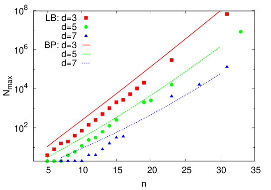
In Fig. 2 we compare this quantity with some known exact results and lower bounds in small dimensions. The maximum rate of packing predicted by the liquid solution of the BP equation is

RBPL1H(δ)+log2[(2ln2)n]n.similar-to-or-equalssuperscript𝑅𝐵𝑃𝐿1𝐻𝛿subscript222𝑛𝑛R^{BPL}\simeq 1-H(\delta)+\frac{\log_{2}[(2\ln 2)n]}{n}. (23)

where we have used

vd2n[1H(δ)].similar-to-or-equalssubscript𝑣𝑑superscript2𝑛delimited-[]1𝐻𝛿v_{d}\simeq 2^{-n[1-H(\delta)]}. (24)

We check the stability of the liquid solution in Appendix A; we find no continuous glass transition as long as

2ln2<14vd,2214subscript𝑣𝑑2\ln 2<\frac{1}{4v_{d}}, (25)

which is the case for δ<12𝛿12\delta<\frac{1}{2} as vdsubscript𝑣𝑑v_{d} is exponentially small in this region.
Refer to caption
Figure 2: Comparing NmaxBPLsuperscriptsubscript𝑁𝑚𝑎𝑥𝐵𝑃𝐿N_{max}^{BPL} (BP) with some lower bounds (LB) from S-amer-1977 . Up to n=15𝑛15n=15 all the lower bounds are exact.

III.0.2 Crystalline solution

In some situations the spheres may prefer one of the sublattices of the Hamming space to the other PZ-jstatphys-2006 . Indeed for even values of d𝑑d, a sphere at the origin forbids more points from the odd sublattice than the even one. For high densities the neighboring spheres will be at distance d𝑑d from the origin, i.e., they occupy points that again belong to the even sublattice. The above observation suggests that we could have ordered states in which nearly all the spheres are in the even or odd sector of the Hamming space. Here we will consider this situation by assigning different messages ηesuperscript𝜂𝑒\eta^{e} and ηosuperscript𝜂𝑜\eta^{o} to points in the even and odd sublattices, respectively. Again we use the fact that all the points in one sublattice are equivalent. Now the BP equations are

ηe=(1VdeηeVdoηo)N22n1[(1VdeηeVdoηo)N2+(1VdeηoVdoηe)N2],superscript𝜂𝑒superscript1subscriptsuperscript𝑉𝑒𝑑superscript𝜂𝑒subscriptsuperscript𝑉𝑜𝑑superscript𝜂𝑜𝑁2superscript2𝑛1delimited-[]superscript1subscriptsuperscript𝑉𝑒𝑑superscript𝜂𝑒subscriptsuperscript𝑉𝑜𝑑superscript𝜂𝑜𝑁2superscript1subscriptsuperscript𝑉𝑒𝑑superscript𝜂𝑜subscriptsuperscript𝑉𝑜𝑑superscript𝜂𝑒𝑁2\displaystyle\eta^{e}=\frac{(1-V^{e}_{d}\eta^{e}-V^{o}_{d}\eta^{o})^{N-2}}{2^{n-1}[(1-V^{e}_{d}\eta^{e}-V^{o}_{d}\eta^{o})^{N-2}+(1-V^{e}_{d}\eta^{o}-V^{o}_{d}\eta^{e})^{N-2}]}, (26)
ηo=(1VdoηeVdeηo)N22n1[(1VdeηeVdoηo)N2+(1VdeηoVdoηe)N2],superscript𝜂𝑜superscript1subscriptsuperscript𝑉𝑜𝑑superscript𝜂𝑒subscriptsuperscript𝑉𝑒𝑑superscript𝜂𝑜𝑁2superscript2𝑛1delimited-[]superscript1subscriptsuperscript𝑉𝑒𝑑superscript𝜂𝑒subscriptsuperscript𝑉𝑜𝑑superscript𝜂𝑜𝑁2superscript1subscriptsuperscript𝑉𝑒𝑑superscript𝜂𝑜subscriptsuperscript𝑉𝑜𝑑superscript𝜂𝑒𝑁2\displaystyle\eta^{o}=\frac{(1-V^{o}_{d}\eta^{e}-V^{e}_{d}\eta^{o})^{N-2}}{2^{n-1}[(1-V^{e}_{d}\eta^{e}-V^{o}_{d}\eta^{o})^{N-2}+(1-V^{e}_{d}\eta^{o}-V^{o}_{d}\eta^{e})^{N-2}]},

where Vdesubscriptsuperscript𝑉𝑒𝑑V^{e}_{d} and Vdosubscriptsuperscript𝑉𝑜𝑑V^{o}_{d} are given by

Vdel=0d11+(1)l2(nl),Vdol=0d11(1)l2(nl).formulae-sequencesubscriptsuperscript𝑉𝑒𝑑superscriptsubscript𝑙0𝑑11superscript1𝑙2𝑛𝑙subscriptsuperscript𝑉𝑜𝑑superscriptsubscript𝑙0𝑑11superscript1𝑙2𝑛𝑙\displaystyle V^{e}_{d}\equiv\sum_{l=0}^{d-1}\frac{1+(-1)^{l}}{2}\left(\begin{array}[]{c}n\\ l\end{array}\right),\hskip 28.45274ptV^{o}_{d}\equiv\sum_{l=0}^{d-1}\frac{1-(-1)^{l}}{2}\left(\begin{array}[]{c}n\\ l\end{array}\right). (31)

Notice that ηe>0superscript𝜂𝑒0\eta^{e}>0 and ηo=0superscript𝜂𝑜0\eta^{o}=0 cannot be a solution of the above equations unless for d=n𝑑𝑛d=n. Indeed to have such a solution we need ηe=12n1=1Vdosuperscript𝜂𝑒1superscript2𝑛11subscriptsuperscript𝑉𝑜𝑑\eta^{e}=\frac{1}{2^{n-1}}=\frac{1}{V^{o}_{d}}, which holds only when d=n𝑑𝑛d=n. We will look for other solutions where ηe>0,ηo>0formulae-sequencesuperscript𝜂𝑒0superscript𝜂𝑜0\eta^{e}>0,\eta^{o}>0. In this case we have

ηe(1VdoηeVdeηo)N2=ηo(1VdeηeVdoηo)N2.superscript𝜂𝑒superscript1subscriptsuperscript𝑉𝑜𝑑superscript𝜂𝑒subscriptsuperscript𝑉𝑒𝑑superscript𝜂𝑜𝑁2superscript𝜂𝑜superscript1subscriptsuperscript𝑉𝑒𝑑superscript𝜂𝑒subscriptsuperscript𝑉𝑜𝑑superscript𝜂𝑜𝑁2\eta^{e}(1-V^{o}_{d}\eta^{e}-V^{e}_{d}\eta^{o})^{N-2}=\eta^{o}(1-V^{e}_{d}\eta^{e}-V^{o}_{d}\eta^{o})^{N-2}. (32)
Refer to caption
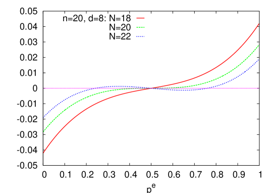
Figure 3: The difference between the two sides of Eq. 33 shows that a crystal solution appears by increasing the number of spheres.

Let us introduce the rescaled variables vdeVde/2n1subscriptsuperscript𝑣𝑒𝑑subscriptsuperscript𝑉𝑒𝑑superscript2𝑛1v^{e}_{d}\equiv V^{e}_{d}/2^{n-1}, vdoVdo/2n1subscriptsuperscript𝑣𝑜𝑑subscriptsuperscript𝑉𝑜𝑑superscript2𝑛1v^{o}_{d}\equiv V^{o}_{d}/2^{n-1}, pe2n1ηesuperscript𝑝𝑒superscript2𝑛1superscript𝜂𝑒p^{e}\equiv 2^{n-1}\eta^{e} and po2n1ηosuperscript𝑝𝑜superscript2𝑛1superscript𝜂𝑜p^{o}\equiv 2^{n-1}\eta^{o}. Using the normalization condition pe+po=1superscript𝑝𝑒superscript𝑝𝑜1p^{e}+p^{o}=1, we obtain an equation for pesuperscript𝑝𝑒p^{e},

pe[1vdopevde(1pe)]N2=(1pe)[1vdepevdo(1pe)]N2.superscript𝑝𝑒superscriptdelimited-[]1subscriptsuperscript𝑣𝑜𝑑superscript𝑝𝑒subscriptsuperscript𝑣𝑒𝑑1superscript𝑝𝑒𝑁21superscript𝑝𝑒superscriptdelimited-[]1subscriptsuperscript𝑣𝑒𝑑superscript𝑝𝑒subscriptsuperscript𝑣𝑜𝑑1superscript𝑝𝑒𝑁2p^{e}[1-v^{o}_{d}p^{e}-v^{e}_{d}(1-p^{e})]^{N-2}=(1-p^{e})[1-v^{e}_{d}p^{e}-v^{o}_{d}(1-p^{e})]^{N-2}. (33)

For large n𝑛n and d𝑑d a nontrivial solution appears at N0BPCsuperscriptsubscript𝑁0𝐵𝑃𝐶N_{0}^{BPC}; see Fig. 3. At this point, the two sides of Eq. 33 have the same slope at pe=1/2superscript𝑝𝑒12p^{e}=1/2. Thus we find

N0BPC=2+2νdνdoνde.superscriptsubscript𝑁0𝐵𝑃𝐶22subscript𝜈𝑑subscriptsuperscript𝜈𝑜𝑑subscriptsuperscript𝜈𝑒𝑑N_{0}^{BPC}=2+\frac{2-\nu_{d}}{\nu^{o}_{d}-\nu^{e}_{d}}. (34)

The entropy of the crystalline phase is obtained given Zisubscript𝑍𝑖Z_{i} and Zijsubscript𝑍𝑖𝑗Z_{ij},

Zisubscript𝑍𝑖\displaystyle Z_{i} =2n1[(1vdepevdopo)N1+(1vdepovdope)N1],absentsuperscript2𝑛1delimited-[]superscript1subscriptsuperscript𝑣𝑒𝑑superscript𝑝𝑒subscriptsuperscript𝑣𝑜𝑑superscript𝑝𝑜𝑁1superscript1subscriptsuperscript𝑣𝑒𝑑superscript𝑝𝑜subscriptsuperscript𝑣𝑜𝑑superscript𝑝𝑒𝑁1\displaystyle=2^{n-1}[(1-v^{e}_{d}p^{e}-v^{o}_{d}p^{o})^{N-1}+(1-v^{e}_{d}p^{o}-v^{o}_{d}p^{e})^{N-1}], (35)
Zijsubscript𝑍𝑖𝑗\displaystyle Z_{ij} =1pe(vdepe+vdopo)po(vdepo+vdope).absent1superscript𝑝𝑒subscriptsuperscript𝑣𝑒𝑑superscript𝑝𝑒subscriptsuperscript𝑣𝑜𝑑superscript𝑝𝑜superscript𝑝𝑜subscriptsuperscript𝑣𝑒𝑑superscript𝑝𝑜subscriptsuperscript𝑣𝑜𝑑superscript𝑝𝑒\displaystyle=1-p^{e}(v^{e}_{d}p^{e}+v^{o}_{d}p^{o})-p^{o}(v^{e}_{d}p^{o}+v^{o}_{d}p^{e}). (36)

To get a simple expression for the entropy we do the following approximation: pe=1superscript𝑝𝑒1p^{e}=1 and po=0superscript𝑝𝑜0p^{o}=0. Notice that when d𝑑d is even, vdo>vdesubscriptsuperscript𝑣𝑜𝑑subscriptsuperscript𝑣𝑒𝑑v^{o}_{d}>v^{e}_{d} and from Eq. 33 we see that for large N𝑁N, posuperscript𝑝𝑜p^{o} should be much smaller than pesuperscript𝑝𝑒p^{e}. In this approximation the entropy reads

sln(2n1)+N12ln(1vde).𝑠superscript2𝑛1𝑁121subscriptsuperscript𝑣𝑒𝑑\displaystyle s\approx\ln(2^{n-1})+\frac{N-1}{2}\ln(1-v^{e}_{d}). (37)

This entropy vanishes at

NmaxBPC=12ln(2n1)ln(1vde).subscriptsuperscript𝑁𝐵𝑃𝐶𝑚𝑎𝑥12superscript2𝑛11subscriptsuperscript𝑣𝑒𝑑\displaystyle N^{BPC}_{max}=1-\frac{2\ln(2^{n-1})}{\ln(1-v^{e}_{d})}. (38)

For large n𝑛n the leading term is

NmaxBPCvde(2ln2)n.similar-to-or-equalssubscriptsuperscript𝑁𝐵𝑃𝐶𝑚𝑎𝑥subscriptsuperscript𝑣𝑒𝑑22𝑛\displaystyle N^{BPC}_{max}v^{e}_{d}\simeq(2\ln 2)n. (39)

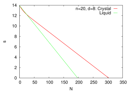
For n,d𝑛𝑑n,d\rightarrow\infty the ratio vd/vdesubscript𝑣𝑑superscriptsubscript𝑣𝑑𝑒v_{d}/v_{d}^{e} approaches to a constant and we recover asymptotically the bound provided with the liquid solution. In Fig. 4 we have compared the liquid and crystal entropies for a given n𝑛n and even d𝑑d. Later in Sec. V.2 we will introduce an iterative algorithm constructing the above crystalline packings.
Refer to caption
Figure 4: Comparing the liquid and crystal entropies predicted by the BP equations.

IV One-step RSB solution: SP equations

In the 1RSB framework we assume that there are an exponentially large number 𝒩ceNΣsimilar-tosubscript𝒩𝑐superscript𝑒𝑁Σ\mathcal{N}_{c}\sim e^{N\Sigma} of clusters of solutions. A cluster of solutions consists of packing solutions in the configuration space that are connected to each other by paths of finite Hamming distances in the thermodynamic limit. In each cluster we could have frozen and unfrozen variables. Suppose the interaction graph is a tree and consider all cavity solutions (in absence of variable j𝑗j) that belong to a given cluster; in a tree graph, fixing the boundary variables is equivalent to fixing the cluster of solutions. It may happen that in all the solutions of a cluster, variable i𝑖i takes only one state, say σ𝜎\sigma. Then the survey bias 𝒰ijsubscript𝒰𝑖𝑗\mathcal{U}_{i\rightarrow j} will be 𝐞σsubscript𝐞𝜎\mathbf{e}_{\sigma} and we say variable i𝑖i is a completely frozen variable in that cluster. We could have partially frozen variables that are frozen on a subset Vfsuperscript𝑉𝑓V^{f} of the Hamming space. In this case we represent the survey bias by 𝒰ij=σVijf𝐞σsubscript𝒰𝑖𝑗subscript𝜎superscriptsubscript𝑉𝑖𝑗𝑓subscript𝐞𝜎\mathcal{U}_{i\rightarrow j}=\sum_{\sigma\in V_{i\rightarrow j}^{f}}\mathbf{e}_{\sigma} ignoring the degeneracy of each state. In general we could write 𝒰ij=σVijfwijσ𝐞σsubscript𝒰𝑖𝑗subscript𝜎superscriptsubscript𝑉𝑖𝑗𝑓superscriptsubscript𝑤𝑖𝑗𝜎subscript𝐞𝜎\mathcal{U}_{i\rightarrow j}=\sum_{\sigma\in V_{i\rightarrow j}^{f}}w_{i\rightarrow j}^{\sigma}\mathbf{e}_{\sigma} where wijσ>0superscriptsubscript𝑤𝑖𝑗𝜎0w_{i\rightarrow j}^{\sigma}>0 is the number of times that variable i𝑖i appears in state σ𝜎\sigma. A variable that takes all possible values is called an unfrozen variable and its survey bias is represented by 𝟎0\mathbf{0}.

The survey biases defined above depend on the cluster of solutions and change from one cluster to another. For an edge (ij)𝑖𝑗(ij) of the interaction graph, we define the histogram of the survey biases among the clusters

𝒬ij(𝒰)=ηij0δ𝒰,𝟎+m=12n1σ1<<σmηijσ1,,σmδ𝒰,σ{σ1,,σm}𝐞σ.subscript𝒬𝑖𝑗𝒰superscriptsubscript𝜂𝑖𝑗0subscript𝛿𝒰0superscriptsubscript𝑚1superscript2𝑛1subscriptsubscript𝜎1subscript𝜎𝑚superscriptsubscript𝜂𝑖𝑗subscript𝜎1subscript𝜎𝑚subscript𝛿𝒰subscript𝜎subscript𝜎1subscript𝜎𝑚subscript𝐞𝜎\displaystyle\mathcal{Q}_{i\rightarrow j}(\mathcal{U})=\eta_{i\rightarrow j}^{0}\delta_{\mathcal{U},\mathbf{0}}+\sum_{m=1}^{2^{n}-1}\sum_{\sigma_{1}<\dots<\sigma_{m}}\eta_{i\rightarrow j}^{\sigma_{1},\dots,\sigma_{m}}\delta_{\mathcal{U},\sum_{\sigma\in\{\sigma_{1},\dots,\sigma_{m}\}}\mathbf{e}_{\sigma}}. (40)

Notice that compared with the RS case here we have the extra option 𝟎0\mathbf{0}. The survey fields are determined by the survey biases:

ijσ=kV(i)jminσVkif{1Iik(σ,σ)}.superscriptsubscript𝑖𝑗𝜎subscript𝑘𝑉𝑖𝑗subscriptsuperscript𝜎superscriptsubscript𝑉𝑘𝑖𝑓1subscript𝐼𝑖𝑘𝜎superscript𝜎\mathcal{H}_{i\rightarrow j}^{\sigma}=\sum_{k\in V(i)\setminus j}\min_{\sigma^{\prime}\in V_{k\rightarrow i}^{f}}\{1-I_{ik}(\sigma,\sigma^{\prime})\}. (41)

In words, ijσsuperscriptsubscript𝑖𝑗𝜎\mathcal{H}_{i\rightarrow j}^{\sigma} is the minimum number of unsatisfied constraints, in the absence of j𝑗j, if sphere i𝑖i takes position σ𝜎\sigma. Here we need only to know if ijσsuperscriptsubscript𝑖𝑗𝜎\mathcal{H}_{i\to j}^{\sigma} is zero or greater than zero. So we change the field’s definition to

ijσ=min{1,kV(i)jminσVkif{1Iik(σ,σ)}}.superscriptsubscript𝑖𝑗𝜎1subscript𝑘𝑉𝑖𝑗subscriptsuperscript𝜎superscriptsubscript𝑉𝑘𝑖𝑓1subscript𝐼𝑖𝑘𝜎superscript𝜎\mathcal{H}_{i\rightarrow j}^{\sigma}=\min\left\{1,\sum_{k\in V(i)\setminus j}\min_{\sigma^{\prime}\in V_{k\rightarrow i}^{f}}\{1-I_{ik}(\sigma,\sigma^{\prime})\}\right\}. (42)

The aim is to write an equation for ηijσ1,,σmsuperscriptsubscript𝜂𝑖𝑗subscript𝜎1subscript𝜎𝑚\eta_{i\rightarrow j}^{\sigma_{1},\ldots,\sigma_{m}}. The value of ηij0superscriptsubscript𝜂𝑖𝑗0\eta_{i\rightarrow j}^{0} is determined by the normalization condition. Variable i𝑖i sends the survey bias 𝒰ij=𝐞σ1++𝐞σmsubscript𝒰𝑖𝑗subscript𝐞subscript𝜎1subscript𝐞subscript𝜎𝑚\mathcal{U}_{i\rightarrow j}=\mathbf{e}_{\sigma_{1}}+\cdots+\mathbf{e}_{\sigma_{m}} to variable j𝑗j if its survey field is

ijσ={0,if σ{σ1,,σm};1,otherwise,superscriptsubscript𝑖𝑗𝜎cases0if σ{σ1,,σm};1otherwise,\mathcal{H}_{i\rightarrow j}^{\sigma}=\left\{\begin{array}[]{ll}0,&\hbox{if $\sigma\in\{\sigma_{1},\ldots,\sigma_{m}\}$;}\\ 1,&\hbox{otherwise,}\end{array}\right. (43)

that is if the only choices for variable i𝑖i are the states in Vf={σ1,,σm}superscript𝑉𝑓subscript𝜎1subscript𝜎𝑚V^{f}=\{\sigma_{1},\ldots,\sigma_{m}\}. We write this probability as

1Prob(σVfijσ=1.OR.σΛVfijσ=0),1-\mathrm{Prob}\left(\bigcup_{\sigma\in V^{f}}\mathcal{H}_{i\rightarrow j}^{\sigma}=1\hskip 5.69054pt\mathrm{.OR.}\hskip 5.69054pt\bigcup_{\sigma\in\Lambda\setminus V^{f}}\mathcal{H}_{i\rightarrow j}^{\sigma}=0\right), (44)

where σijσ=0subscript𝜎superscriptsubscript𝑖𝑗𝜎0\bigcup_{\sigma}\mathcal{H}_{i\rightarrow j}^{\sigma}=0 is the event that at least one of the ijσsuperscriptsubscript𝑖𝑗𝜎\mathcal{H}_{i\rightarrow j}^{\sigma} is zero. We have also the condition that variable i𝑖i dose not receive contradictory biases. It means that the cavity field ijsubscript𝑖𝑗\mathcal{H}_{i\rightarrow j} should not be equal to 𝟏(1,,1)111\mathbf{1}\equiv(1,\ldots,1). This probability is given by Prob(σijσ=0)Probsubscript𝜎superscriptsubscript𝑖𝑗𝜎0\mathrm{Prob}\left(\bigcup_{\sigma}\mathcal{H}_{i\rightarrow j}^{\sigma}=0\right); so we obtain

ηijσ1,,σm=1Prob(σVfijσ=1.OR.σΛVfijσ=0)Prob(σijσ=0).\eta_{i\rightarrow j}^{\sigma_{1},\ldots,\sigma_{m}}=\frac{1-\mathrm{Prob}\left(\bigcup_{\sigma\in V^{f}}\mathcal{H}_{i\rightarrow j}^{\sigma}=1\hskip 5.69054pt\mathrm{.OR.}\hskip 5.69054pt\bigcup_{\sigma\in\Lambda\setminus V^{f}}\mathcal{H}_{i\rightarrow j}^{\sigma}=0\right)}{\mathrm{Prob}\left(\bigcup_{\sigma}\mathcal{H}_{i\rightarrow j}^{\sigma}=0\right)}. (45)

One can use the standard tools in the probability theory to find the above probabilities in terms of η𝜂\eta’s. The result is the so called SP equation and is derived with more details in Appendix B. Here we simplify the analysis by assuming that all partially frozen surveys are zero, that is, only completely frozen and unfrozen surveys are taken into account. This would be a reasonable approximation when N𝑁N approaches Nmaxsubscript𝑁𝑚𝑎𝑥N_{max}. We also expect to obtain a larger complexity within this approximation. In this ansatz the SP equation reads

ηijσ=m=02n1(1)mσ1<<σmΛσkV(i)j(1σV(σ,σ1,,σm)ηkiσ)m=12n(1)m+1σ1<<σmkV(i)j(1σV(σ1,,σm)ηkiσ),superscriptsubscript𝜂𝑖𝑗𝜎superscriptsubscript𝑚0superscript2𝑛1superscript1𝑚subscriptsubscript𝜎1subscript𝜎𝑚Λ𝜎subscriptproduct𝑘𝑉𝑖𝑗1subscriptsuperscript𝜎subscript𝑉𝜎subscript𝜎1subscript𝜎𝑚superscriptsubscript𝜂𝑘𝑖superscript𝜎superscriptsubscript𝑚1superscript2𝑛superscript1𝑚1subscriptsubscript𝜎1subscript𝜎𝑚subscriptproduct𝑘𝑉𝑖𝑗1subscriptsuperscript𝜎subscript𝑉subscript𝜎1subscript𝜎𝑚superscriptsubscript𝜂𝑘𝑖superscript𝜎\eta_{i\rightarrow j}^{\sigma}=\frac{\sum_{m=0}^{2^{n}-1}(-1)^{m}\sum_{\sigma_{1}<\dots<\sigma_{m}\in\Lambda\setminus\sigma}\prod_{k\in V(i)\setminus j}\left(1-\sum_{\sigma^{\prime}\in V_{\cup}(\sigma,\sigma_{1},\dots,\sigma_{m})}\eta_{k\rightarrow i}^{\sigma^{\prime}}\right)}{\sum_{m=1}^{2^{n}}(-1)^{m+1}\sum_{\sigma_{1}<\dots<\sigma_{m}}\prod_{k\in V(i)\setminus j}\left(1-\sum_{\sigma^{\prime}\in V_{\cup}(\sigma_{1},\dots,\sigma_{m})}\eta_{k\rightarrow i}^{\sigma^{\prime}}\right)}, (46)

where V(σ1,,σm)subscript𝑉subscript𝜎1subscript𝜎𝑚V_{\cup}(\sigma_{1},\ldots,\sigma_{m}) is the union volume of Vd(σ1)subscript𝑉𝑑subscript𝜎1V_{d}(\sigma_{1}), Vd(σ2)subscript𝑉𝑑subscript𝜎2V_{d}(\sigma_{2}), \ldots and Vd(σm)subscript𝑉𝑑subscript𝜎𝑚V_{d}(\sigma_{m}).

In our problem all the edges of the interaction graph are equivalent. Moreover, due to the translational symmetry, the surveys ηijσsuperscriptsubscript𝜂𝑖𝑗𝜎\eta_{i\rightarrow j}^{\sigma} do not depend on σ𝜎\sigma. Considering these simplifications, the SP equation can be rewritten in a more compact form as

η=12nV=Vd2nG(V)(1Vη)N2V=Vd2nG(V)(1Vη)N2,𝜂1superscript2𝑛superscriptsubscript𝑉subscript𝑉𝑑superscript2𝑛superscript𝐺𝑉superscript1𝑉𝜂𝑁2superscriptsubscript𝑉subscript𝑉𝑑superscript2𝑛𝐺𝑉superscript1𝑉𝜂𝑁2\eta=\frac{1}{2^{n}}\frac{\sum_{V=V_{d}}^{2^{n}}G^{\prime}(V)(1-V\eta)^{N-2}}{\sum_{V=V_{d}}^{2^{n}}G(V)(1-V\eta)^{N-2}}, (47)

where

G(V)=m=12n(1)m+1gm(V),G(V)=m=12n(1)m+1mgm(V).formulae-sequence𝐺𝑉superscriptsubscript𝑚1superscript2𝑛superscript1𝑚1subscript𝑔𝑚𝑉superscript𝐺𝑉superscriptsubscript𝑚1superscript2𝑛superscript1𝑚1𝑚subscript𝑔𝑚𝑉\displaystyle G(V)=\sum_{m=1}^{2^{n}}(-1)^{m+1}g_{m}(V),\hskip 28.45274ptG^{\prime}(V)=\sum_{m=1}^{2^{n}}(-1)^{m+1}mg_{m}(V). (48)

Here gm(V)subscript𝑔𝑚𝑉g_{m}(V) is the total number of configurations that m𝑚m distinct points can take in the Hamming space such that the union volume Vsubscript𝑉V_{\cup} is equal to V𝑉V. More precisely we have

gm(V)=σ1<<σmδV,V(σ1,,σm).subscript𝑔𝑚𝑉subscriptsubscript𝜎1subscript𝜎𝑚subscript𝛿𝑉subscript𝑉subscript𝜎1subscript𝜎𝑚g_{m}(V)=\sum_{\sigma_{1}<\dots<\sigma_{m}}\delta_{V,V_{\cup}(\sigma_{1},\ldots,\sigma_{m})}. (49)

To obtain more explicit results we consider a naive approximation where V(σ1,,σm)mVdsubscript𝑉subscript𝜎1subscript𝜎𝑚𝑚subscript𝑉𝑑V_{\cup}(\sigma_{1},\ldots,\sigma_{m})\approx mV_{d}. This is a good approximation for small d/n𝑑𝑛d/n. We also approximate (1mVdη)N2superscript1𝑚subscript𝑉𝑑𝜂𝑁2(1-mV_{d}\eta)^{N-2} by e(N2)mVdηsuperscript𝑒𝑁2𝑚subscript𝑉𝑑𝜂e^{-(N-2)mV_{d}\eta} to compensate the error made by overestimating the union volume V(σ1,,σm)subscript𝑉subscript𝜎1subscript𝜎𝑚V_{\cup}(\sigma_{1},\ldots,\sigma_{m}) for large m𝑚m. Then the SP equation reads

η=12nm=12nm(1)m1(2nm)em(N2)Vdηm=12n(1)m1(2nm)em(N2)Vdη.𝜂1superscript2𝑛superscriptsubscript𝑚1superscript2𝑛𝑚superscript1𝑚1superscript2𝑛𝑚superscript𝑒𝑚𝑁2subscript𝑉𝑑𝜂superscriptsubscript𝑚1superscript2𝑛superscript1𝑚1superscript2𝑛𝑚superscript𝑒𝑚𝑁2subscript𝑉𝑑𝜂\eta=\frac{1}{2^{n}}\frac{\sum_{m=1}^{2^{n}}m(-1)^{m-1}\left(\begin{array}[]{c}2^{n}\\ m\end{array}\right)e^{-m(N-2)V_{d}\eta}}{\sum_{m=1}^{2^{n}}(-1)^{m-1}\left(\begin{array}[]{c}2^{n}\\ m\end{array}\right)e^{-m(N-2)V_{d}\eta}}. (50)

Summing over m𝑚m we get

η=e(N2)Vdη(1e(N2)Vdη)2n11(1e(N2)Vdη)2n.𝜂superscript𝑒𝑁2subscript𝑉𝑑𝜂superscript1superscript𝑒𝑁2subscript𝑉𝑑𝜂superscript2𝑛11superscript1superscript𝑒𝑁2subscript𝑉𝑑𝜂superscript2𝑛\eta=\frac{e^{-(N-2)V_{d}\eta}(1-e^{-(N-2)V_{d}\eta})^{2^{n}-1}}{1-(1-e^{-(N-2)V_{d}\eta})^{2^{n}}}. (51)

Let us see where the above equation admits a nontrivial solution η>0𝜂0\eta>0. To this end we will consider the following scalings: (N2)Vd/2n=cn𝑁2subscript𝑉𝑑superscript2𝑛𝑐𝑛(N-2)V_{d}/2^{n}=cn and 2nη=1g(n,c)superscript2𝑛𝜂1𝑔𝑛𝑐2^{n}\eta=1-g(n,c). For n𝑛n\rightarrow\infty we expect to have cconst𝑐constc\rightarrow\mathrm{const} and g0𝑔0g\rightarrow 0. Replacing these in the above equation and expanding for small 2necn(1g)superscript2𝑛superscript𝑒𝑐𝑛1𝑔2^{n}e^{-cn(1-g)} we obtain

g2necn(1g).similar-to-or-equals𝑔superscript2𝑛superscript𝑒𝑐𝑛1𝑔g\simeq 2^{n}e^{-cn(1-g)}. (52)

To have a solution for g𝑔g we need c>ln2+c(lnn)/n𝑐2superscript𝑐𝑛𝑛c>\ln 2+c^{\prime}(\ln n)/n with

(nln2+clnn)eclnn=1.𝑛2superscript𝑐𝑛superscript𝑒superscript𝑐𝑛1(n\ln 2+c^{\prime}\ln n)e^{-c^{\prime}\ln n}=1. (53)

Increasing N𝑁N, the frozen variables appear for the first time at NcSPsuperscriptsubscript𝑁𝑐𝑆𝑃N_{c}^{SP}, where

c1+O(1lnn),cln2+lnnn+O(1n),formulae-sequencesimilar-to-or-equalssuperscript𝑐1𝑂1𝑛similar-to-or-equals𝑐2𝑛𝑛𝑂1𝑛\displaystyle c^{\prime}\simeq 1+O\left(\frac{1}{\ln n}\right),\hskip 28.45274ptc\simeq\ln 2+\frac{\ln n}{n}+O\left(\frac{1}{n}\right), (54)

and therefore

NcSPvdnln2+lnn+const.similar-to-or-equalssuperscriptsubscript𝑁𝑐𝑆𝑃subscript𝑣𝑑𝑛2𝑛constN_{c}^{SP}v_{d}\simeq n\ln 2+\ln n+\mathrm{const}. (55)

This gives the clustering transition, when the solution space splits into an exponentially large number of clusters.

IV.0.1 Complexity

We can compute the complexity in the Bethe approximation as

Σ=1N[iΔΣii<jΔΣij].Σ1𝑁delimited-[]subscript𝑖ΔsubscriptΣ𝑖subscript𝑖𝑗ΔsubscriptΣ𝑖𝑗\Sigma=\frac{1}{N}\left[\sum_{i}\Delta\Sigma_{i}-\sum_{i<j}\Delta\Sigma_{ij}\right]. (56)

As before, ΔΣiΔsubscriptΣ𝑖\Delta\Sigma_{i} and ΔΣijΔsubscriptΣ𝑖𝑗\Delta\Sigma_{ij} are the complexity shifts by adding variable i𝑖i and interaction (ij)𝑖𝑗(ij). The complexity is zero for small densities of the particles where we expect to have a single cluster of solutions. As we increase N𝑁N, we encounter the clustering transition at Ncsubscript𝑁𝑐N_{c}, where ΣΣ\Sigma becomes nonzero. The complexity is a decreasing function of N𝑁N and finally vanishes at Nmaxsubscript𝑁𝑚𝑎𝑥N_{max}. Here we shall focus on the most numerous clusters, which are not necessarily the relevant ones. More accurate results can be obtained by a large deviation study of the problem, which involves computing the complexity of different clusters KMRSZ-pnas-2007 .

To compute the complexity we need the two quantities ΔΣiΔsubscriptΣ𝑖\Delta\Sigma_{i} and ΔΣijΔsubscriptΣ𝑖𝑗\Delta\Sigma_{ij}. Again for the sake of simplicity we only work with the completely frozen surveys. In this approximation we get

eΔΣi=m=12n(1)m+1σ1<<σmjV(i)(1σV(σ1,,σm)ηjiσ)𝒵i,superscript𝑒ΔsubscriptΣ𝑖superscriptsubscript𝑚1superscript2𝑛superscript1𝑚1subscriptsubscript𝜎1subscript𝜎𝑚subscriptproduct𝑗𝑉𝑖1subscriptsuperscript𝜎subscript𝑉subscript𝜎1subscript𝜎𝑚superscriptsubscript𝜂𝑗𝑖superscript𝜎subscript𝒵𝑖e^{\Delta\Sigma_{i}}=\sum_{m=1}^{2^{n}}(-1)^{m+1}\sum_{\sigma_{1}<\dots<\sigma_{m}}\prod_{j\in V(i)}\left(1-\sum_{\sigma^{\prime}\in V_{\cup}(\sigma_{1},\ldots,\sigma_{m})}\eta_{j\rightarrow i}^{\sigma^{\prime}}\right)\equiv\mathcal{Z}_{i}, (57)

and the link contribution is

eΔΣij=1σ,σ:D(σ,σ)<dηijσηjiσ𝒵ij.superscript𝑒ΔsubscriptΣ𝑖𝑗1subscript:𝜎superscript𝜎𝐷𝜎superscript𝜎𝑑superscriptsubscript𝜂𝑖𝑗𝜎superscriptsubscript𝜂𝑗𝑖superscript𝜎subscript𝒵𝑖𝑗e^{\Delta\Sigma_{ij}}=1-\sum_{\sigma,\sigma^{\prime}:D(\sigma,\sigma^{\prime})<d}\eta_{i\rightarrow j}^{\sigma}\eta_{j\rightarrow i}^{\sigma^{\prime}}\equiv\mathcal{Z}_{ij}. (58)

Using our notation in the previous subsection we can write a more compact form of the complexity for uniform surveys

Σ=ln[VG(V)(1Vη)N1]N12ln[12nVdη2].Σsubscript𝑉𝐺𝑉superscript1𝑉𝜂𝑁1𝑁121superscript2𝑛subscript𝑉𝑑superscript𝜂2\displaystyle\Sigma=\ln\left[\sum_{V}G(V)(1-V\eta)^{N-1}\right]-\frac{N-1}{2}\ln[1-2^{n}V_{d}\eta^{2}]. (59)

In the naive approximation, where we approximate Vsubscript𝑉V_{\cup} by mVd𝑚subscript𝑉𝑑mV_{d}, we find

Σ=ln[1(1e(N1)Vdη)2n]N12ln[12nVdη2].Σ1superscript1superscript𝑒𝑁1subscript𝑉𝑑𝜂superscript2𝑛𝑁121superscript2𝑛subscript𝑉𝑑superscript𝜂2\Sigma=\ln[1-(1-e^{-(N-1)V_{d}\eta})^{2^{n}}]-\frac{N-1}{2}\ln[1-2^{n}V_{d}\eta^{2}]. (60)

The complexity vanishes when

1(1e(N1)Vdη)2n=(12nVdη2)N12.1superscript1superscript𝑒𝑁1subscript𝑉𝑑𝜂superscript2𝑛superscript1superscript2𝑛subscript𝑉𝑑superscript𝜂2𝑁121-(1-e^{-(N-1)V_{d}\eta})^{2^{n}}=(1-2^{n}V_{d}\eta^{2})^{\frac{N-1}{2}}. (61)

Using again the scalings (N1)Vd/2n=cn𝑁1subscript𝑉𝑑superscript2𝑛𝑐𝑛(N-1)V_{d}/2^{n}=cn and 2nη=1g(c,n)superscript2𝑛𝜂1𝑔𝑐𝑛2^{n}\eta=1-g(c,n), the above equation can be rewritten as

1ex=e12cn(1g)2,xen[ln2c(1g)].formulae-sequence1superscript𝑒𝑥superscript𝑒12𝑐𝑛superscript1𝑔2𝑥superscript𝑒𝑛delimited-[]2𝑐1𝑔1-e^{-x}=e^{-\frac{1}{2}cn(1-g)^{2}},\hskip 28.45274ptx\equiv e^{n[\ln 2-c(1-g)]}. (62)

Expanding the left side for the exponentially small x𝑥x we obtain

2ln2=c(1g2).22𝑐1superscript𝑔22\ln 2=c(1-g^{2}). (63)

Notice that g𝑔g approaches to zero for large n𝑛n as 1/n1𝑛1/n, so the above equation suggests

NmaxSPvd=(2ln2)n+O(1/n).superscriptsubscript𝑁𝑚𝑎𝑥𝑆𝑃subscript𝑣𝑑22𝑛𝑂1𝑛N_{max}^{SP}v_{d}=(2\ln 2)n+O(1/n). (64)

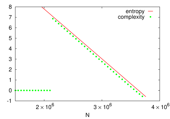
Using Eqs. 51 and 60 we can find the complexity in the naive approximation. In Fig. 5 we have compared this complexity with the BP entropy for n=25𝑛25n=25 and d=2𝑑2d=2, where the naive approximation is expected to work. We see the jump in the complexity that happens at the clustering transition NcSPsuperscriptsubscript𝑁𝑐𝑆𝑃N_{c}^{SP}. Moreover, the complexity is always smaller than the RS entropy, as it should be; it is the sum Σ+sclusterΣsubscript𝑠𝑐𝑙𝑢𝑠𝑡𝑒𝑟\Sigma+s_{cluster} that gives the total entropy of the system. Here sclustersubscript𝑠𝑐𝑙𝑢𝑠𝑡𝑒𝑟s_{cluster} is the internal entropy of the clusters.
Refer to caption
Figure 5: Comparing the RS entropy with the 1RSB complexity in the naive approximation. Here n=25𝑛25n=25 and d=2𝑑2d=2.

Let us summarize the main approximations we used in the above calculations: First, the SP equation ignores the soft part of the messages and works only with the hard fields. We know that this could give an underestimate of the clustering transition but works well in predicting the satisfiability-unsatisfiability (SAT-UNSAT) transition in some constraint satisfaction problems. Next, we neglected the partially frozen states and considered only the completely frozen and unfrozen parts to write a simpler expression for the SP equation. This approximation seems reasonable as for maximum packings the spheres should be strongly localized by their neighborhood. And finally, we resorted to another approximation by replacing the union volume of m𝑚m distinct spheres with mVd𝑚subscript𝑉𝑑mV_{d}. One can improve on this by using an annealed approximation of Vsubscript𝑉V_{\cup},

V(σ1,,σm)2n[1(1vd)m],similar-to-or-equalssubscript𝑉subscript𝜎1subscript𝜎𝑚superscript2𝑛delimited-[]1superscript1subscript𝑣𝑑𝑚V_{\cup}(\sigma_{1},\ldots,\sigma_{m})\simeq 2^{n}[1-(1-v_{d})^{m}], (65)

where (1vd)msuperscript1subscript𝑣𝑑𝑚(1-v_{d})^{m} is the probability that a point in the Hamming space is outside the m𝑚m spheres centered at σ1subscript𝜎1\sigma_{1}, \ldots, σmsubscript𝜎𝑚\sigma_{m}. Further, we can approximate gm(V)subscript𝑔𝑚𝑉g_{m}(V) by

gm(V)(2nm)(2nV)[1(1vd)m]V[(1vd)m]2nV.similar-to-or-equalssubscript𝑔𝑚𝑉superscript2𝑛𝑚superscript2𝑛𝑉superscriptdelimited-[]1superscript1subscript𝑣𝑑𝑚𝑉superscriptdelimited-[]superscript1subscript𝑣𝑑𝑚superscript2𝑛𝑉\displaystyle g_{m}(V)\simeq\left(\begin{array}[]{c}2^{n}\\ m\end{array}\right)\left(\begin{array}[]{c}2^{n}\\ V\end{array}\right)[1-(1-v_{d})^{m}]^{V}[(1-v_{d})^{m}]^{2^{n}-V}. (70)

The annealed volume is approximately given by mVd𝑚subscript𝑉𝑑mV_{d} when m2nVdmuch-less-than𝑚superscript2𝑛subscript𝑉𝑑m\ll\frac{2^{n}}{V_{d}}. Moreover, the completely frozen approximation we used, suggests that the main contribution in the SP equation comes from small values of m𝑚m, see Appendix B. Therefore, we do not expect to observe exponentially large deviations in NcSPsuperscriptsubscript𝑁𝑐𝑆𝑃N_{c}^{SP} and NmaxSPsuperscriptsubscript𝑁𝑚𝑎𝑥𝑆𝑃N_{max}^{SP} beyond the naive approximation.

V Some algorithms for the packing problem

V.1 Hard spheres in an ultrametric space

Exact solutions are always useful in that we obtain some insights about more complex problems TS-pre-2006 ; TS-em-2006 . As a simple example which can be treated exactly, we consider the packing problem in an ultrametric space.

An ultrametric space is a metric space where for any three points i1,i2,subscript𝑖1subscript𝑖2i_{1},i_{2}, and i3subscript𝑖3i_{3} we have D(i1,i2)max{D(i1,i3),D(i2,i3)}𝐷subscript𝑖1subscript𝑖2𝐷subscript𝑖1subscript𝑖3𝐷subscript𝑖2subscript𝑖3D(i_{1},i_{2})\leq\max\{D(i_{1},i_{3}),D(i_{2},i_{3})\}. Consider a rooted binary tree 𝖳nsubscript𝖳𝑛\mathsf{T}_{n} with n𝑛n generations. The number of points at generation l𝑙l is 2lsuperscript2𝑙2^{l}. The space of points is given by the 2nsuperscript2𝑛2^{n} leaves of this tree. The distance D(i1,i2)𝐷subscript𝑖1subscript𝑖2D(i_{1},i_{2}) between two points i1subscript𝑖1i_{1} and i2subscript𝑖2i_{2} is defined as the number of generations that one should go up in the tree to find the first common ancestor.

Refer to caption
Figure 6: Packing hard spheres in an ultra-metric space. Here n1=2subscript𝑛12n_{1}=2 and N=22𝑁superscript22N=2^{2}. Filled and empty spheres show valid packings for d=1𝑑1d=1 and d=2𝑑2d=2, respectively.

The problem is to find a packing of N𝑁N hard spheres such that for any two spheres D(i1,i2)d𝐷subscript𝑖1subscript𝑖2𝑑D(i_{1},i_{2})\geq d. The packing problem is trivial for d=1𝑑1d=1, so we can start from this simple case and try to find packings for larger d𝑑d. Let us start with a binary tree of n1subscript𝑛1n_{1} generations and 2n1superscript2subscript𝑛12^{n_{1}} leaves, 𝖳n1subscript𝖳subscript𝑛1\mathsf{T}_{n_{1}}. We put one sphere at each point of this ultrametric space to obtain a packing of N=2n1𝑁superscript2subscript𝑛1N=2^{n_{1}} spheres with diameter d=1𝑑1d=1; see Fig. 6. This is the densest configuration of hard spheres for the above parameters. The idea is to increase d𝑑d by 111 and add the minimum number of necessary generations to find a new packing with the new diameter for the spheres. Indeed in an ultrametric space we need only one additional generation to remove all the overlaps in the previous configuration. After adding the new generation we are free to put each sphere in one of its two descendants. One can continue the above process to find a valid packing for an arbitrary value of d𝑑d. It turns out that these are the densest configurations of the spheres with the parameters n𝑛n and d𝑑d; the packing indeed partitions the whole space into regions occupied by the spheres. Therefore, given n𝑛n and d𝑑d, the number of packings and maximum number of spheres read

Z=N!(2ndN)(2d)N,Nmax=2nd.formulae-sequence𝑍𝑁superscript2𝑛𝑑𝑁superscriptsuperscript2𝑑𝑁subscript𝑁𝑚𝑎𝑥superscript2𝑛𝑑\displaystyle Z=N!\left(\begin{array}[]{c}2^{n-d}\\ N\end{array}\right)(2^{d})^{N},\hskip 28.45274ptN_{max}=2^{n-d}. (73)

The maximum rate of packing will be

RUM=log2Nmaxn=1δ.superscript𝑅𝑈𝑀subscript2subscript𝑁𝑚𝑎𝑥𝑛1𝛿\displaystyle R^{UM}=\frac{\log_{2}N_{max}}{n}=1-\delta. (74)

It is interesting that this is exactly the Shannon rate for a binary erasure channel with error probability δ𝛿\delta.

The above example is one of the exactly solvable packing problems that one can compare the exact Nmaxsubscript𝑁𝑚𝑎𝑥N_{max} with the BP one computed at the liquid solution:

NmaxBPL=1(2ln2)nln(12dn)(2ln2)n2nd.superscriptsubscript𝑁𝑚𝑎𝑥𝐵𝑃𝐿122𝑛1superscript2𝑑𝑛22𝑛superscript2𝑛𝑑\displaystyle N_{max}^{BPL}=1-\frac{(2\ln 2)n}{\ln(1-2^{d-n})}\to(2\ln 2)n2^{n-d}. (75)

Here NmaxBPL>Nmaxsuperscriptsubscript𝑁𝑚𝑎𝑥𝐵𝑃𝐿subscript𝑁𝑚𝑎𝑥N_{max}^{BPL}>N_{max} but we find asymptotically RBPL=1δsuperscript𝑅𝐵𝑃𝐿1𝛿R^{BPL}=1-\delta.

V.2 Hard spheres in the Hamming space

Here we can use the same strategy as above to find packings of hard spheres in the Hamming space. The points of an n𝑛n-dimensional Hamming space can be represented by the leaves of a binary tree 𝖳nsubscript𝖳𝑛\mathsf{T}_{n}. A configuration of N𝑁N spheres, σ¯{σiΛ|i=1,,N}¯𝜎conditional-setsubscript𝜎𝑖Λ𝑖1𝑁\underline{\sigma}\equiv\{\sigma_{i}\in\Lambda|i=1,\ldots,N\}, is a packing of hard spheres with diameter d𝑑d if it satisfies the following set of constraints

𝒞(d){D(σi,σj)d|ij},𝒞𝑑conditional-set𝐷subscript𝜎𝑖subscript𝜎𝑗𝑑𝑖𝑗\mathcal{C}(d)\equiv\left\{D(\sigma_{i},\sigma_{j})\geq d|i\neq j\right\}, (76)

where D(σi,σj)𝐷subscript𝜎𝑖subscript𝜎𝑗D(\sigma_{i},\sigma_{j}) is the Hamming distance of points σisubscript𝜎𝑖\sigma_{i} and σjsubscript𝜎𝑗\sigma_{j}. We define the energy E[σ¯]=i<j[1Iij(σi,σj)]𝐸delimited-[]¯𝜎subscript𝑖𝑗delimited-[]1subscript𝐼𝑖𝑗subscript𝜎𝑖subscript𝜎𝑗E[\underline{\sigma}]=\sum_{i<j}[1-I_{ij}(\sigma_{i},\sigma_{j})] as the number of unsatisfied constraints. The conflict graph 𝒢(σ¯)𝒢¯𝜎\mathcal{G}(\underline{\sigma}) represents a graph of N𝑁N nodes where edge (ij)𝑖𝑗(ij) is present if the corresponding constraint is not satisfied. To find a packing we do the following steps:

  • We start with N=2n1𝑁superscript2subscript𝑛1N=2^{n_{1}} spheres occupying all the leaves of 𝖳n1subscript𝖳subscript𝑛1\mathsf{T}_{n_{1}}. This is the densest configuration of spheres that satisfies 𝒞(1)𝒞1\mathcal{C}(1). We use σ¯1superscript¯𝜎1\underline{\sigma}^{1} to represent this configuration of spheres.

  • For t=2,,d𝑡2𝑑t=2,\ldots,d, we start with (σ¯t1,𝖳nt1)superscript¯𝜎𝑡1subscript𝖳subscript𝑛𝑡1(\underline{\sigma}^{t-1},\mathsf{T}_{n_{t-1}}) and find (σ¯t,𝖳nt)superscript¯𝜎𝑡subscript𝖳subscript𝑛𝑡(\underline{\sigma}^{t},\mathsf{T}_{n_{t}}) such that all the constraints in 𝒞(t)𝒞𝑡\mathcal{C}(t) are satisfied. Set n=nt1𝑛subscript𝑛𝑡1n=n_{t-1} and Δnt=0Δsubscript𝑛𝑡0\Delta n_{t}=0, then

    • If E>0𝐸0E>0, add a new generation to 𝖳nsubscript𝖳𝑛\mathsf{T}_{n}, that is n=n+1𝑛𝑛1n=n+1 and Δnt=Δnt+1Δsubscript𝑛𝑡Δsubscript𝑛𝑡1\Delta n_{t}=\Delta n_{t}+1.

    • For each sphere find the best value of σi(n){0,1}subscript𝜎𝑖𝑛01\sigma_{i}(n)\in\{0,1\} and call the new configuration σ¯t1,Δntsuperscript¯𝜎𝑡1Δsubscript𝑛𝑡\underline{\sigma}^{t-1,\Delta n_{t}}. If E=0𝐸0E=0 return σ¯t=σ¯t1,Δntsuperscript¯𝜎𝑡superscript¯𝜎𝑡1Δsubscript𝑛𝑡\underline{\sigma}^{t}=\underline{\sigma}^{t-1,\Delta n_{t}} and nt=nsubscript𝑛𝑡𝑛n_{t}=n.

Refer to caption
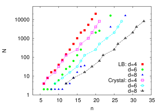
Figure 7: Comparing number of spheres in the crystalline packings generated by the iterative algorithm with some lower bounds (LB) from S-amer-1977 . Up to n=15𝑛15n=15 all the lower bounds are exact.

Notice that every time we add a new generation we have to solve an optimization problem to find the best configuration, s¯{σi(n)|i=1,,N}¯𝑠conditional-setsubscript𝜎𝑖𝑛𝑖1𝑁\underline{s}\equiv\{\sigma_{i}(n)|i=1,\ldots,N\}. Given t𝑡t and ΔntΔsubscript𝑛𝑡\Delta n_{t}, we need to find the ground state of the following energy function

E[s¯]=(ij)𝒢(σ¯t1,Δnt)δsi,sj.𝐸delimited-[]¯𝑠subscript𝑖𝑗𝒢superscript¯𝜎𝑡1Δsubscript𝑛𝑡subscript𝛿subscript𝑠𝑖subscript𝑠𝑗E[\underline{s}]=\sum_{(ij)\in\mathcal{G}(\underline{\sigma}^{t-1,\Delta n_{t}})}\delta_{s_{i},s_{j}}. (77)

The aim is to assign different values to the new components sisubscript𝑠𝑖s_{i} and sjsubscript𝑠𝑗s_{j} when edge (ij)𝑖𝑗(ij) belongs to the conflict graph. In our numerical simulations we use simulated annealing to solve the above optimization problem.

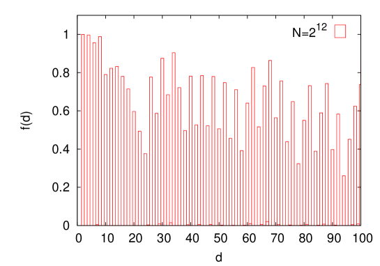
We observe that for even t𝑡t the change in the number of generations ΔntΔsubscript𝑛𝑡\Delta n_{t} is 111; i.e., the conflict graph is a bipartite graph connecting only spheres in different sublattices, odd and even. Consequently, for even d𝑑d all spheres are in the same sublattice of the Hamming space, as expected from the crystalline phase of Sec. III.0.2. In Fig. 7 we have compared the packings constructed by the above algorithm with the known lower bounds. We also checked the fraction of locally frozen spheres in these packings. A locally frozen sphere is one that, fixing the other spheres, cannot be locally displaced without violating some of the constraints. Figure 8 displays this quantity as a function of d𝑑d. We see that for even d𝑑d a considerable fraction of the spheres are frozen. This indicates that finding such packings is very difficult by a random sequential adding algorithm T-springer-2002 where spheres are added randomly one by one.
Refer to caption
Figure 8: Fraction of locally frozen spheres in the packings generated by the iterative algorithm.

V.3 An algorithm based on the BP equations

Let us again write the general BP equations for the packing problem:

ηij(σi)kV(i)j(σkIik(σi,σk)ηki(σk)).proportional-tosubscript𝜂𝑖𝑗subscript𝜎𝑖subscriptproduct𝑘𝑉𝑖𝑗subscriptsubscript𝜎𝑘subscript𝐼𝑖𝑘subscript𝜎𝑖subscript𝜎𝑘subscript𝜂𝑘𝑖subscript𝜎𝑘\displaystyle\eta_{i\rightarrow j}(\sigma_{i})\propto\prod_{k\in V(i)\setminus j}\left(\sum_{\sigma_{k}}I_{ik}(\sigma_{i},\sigma_{k})\eta_{k\rightarrow i}(\sigma_{k})\right). (78)

To solve these equations one starts with random initial values for the cavity messages and updates the messages iteratively to reach a fixed point. At the fixed point we have the local marginals given by

ηi(σi)jV(i)(σjIij(σi,σj)ηji(σj)).proportional-tosubscript𝜂𝑖subscript𝜎𝑖subscriptproduct𝑗𝑉𝑖subscriptsubscript𝜎𝑗subscript𝐼𝑖𝑗subscript𝜎𝑖subscript𝜎𝑗subscript𝜂𝑗𝑖subscript𝜎𝑗\displaystyle\eta_{i}(\sigma_{i})\propto\prod_{j\in V(i)}\left(\sum_{\sigma_{j}}I_{ij}(\sigma_{i},\sigma_{j})\eta_{j\rightarrow i}(\sigma_{j})\right). (79)

One can find a packing configuration by decimation, fixing the spheres one by one according to the above local marginals; after each decimation one has to run again the BP equations to obtained the new marginals. Here we take another approach, by using the local marginals to converge the equations to a polarized fixed point defining a packing configuration. We found it useful here to add also some additional random potential wi(σi)subscript𝑤𝑖subscript𝜎𝑖w_{i}(\sigma_{i}) to break the high level of symmetry present in the problem. The modified BP equations read

ηij(σi)subscript𝜂𝑖𝑗subscript𝜎𝑖\displaystyle\eta_{i\rightarrow j}(\sigma_{i}) [ηi(σi)]reβwi(σi)kV(i)j(σkIik(σi,σk)ηki(σk)),proportional-toabsentsuperscriptdelimited-[]subscript𝜂𝑖subscript𝜎𝑖𝑟superscript𝑒𝛽subscript𝑤𝑖subscript𝜎𝑖subscriptproduct𝑘𝑉𝑖𝑗subscriptsubscript𝜎𝑘subscript𝐼𝑖𝑘subscript𝜎𝑖subscript𝜎𝑘subscript𝜂𝑘𝑖subscript𝜎𝑘\displaystyle\propto[\eta_{i}(\sigma_{i})]^{r}e^{\beta w_{i}(\sigma_{i})}\prod_{k\in V(i)\setminus j}\left(\sum_{\sigma_{k}}I_{ik}(\sigma_{i},\sigma_{k})\eta_{k\to i}(\sigma_{k})\right), (80)
ηi(σi)subscript𝜂𝑖subscript𝜎𝑖\displaystyle\eta_{i}(\sigma_{i}) [ηi(σi)]reβwi(σi)jV(i)(σjIij(σi,σj)ηji(σj)),proportional-toabsentsuperscriptdelimited-[]subscript𝜂𝑖subscript𝜎𝑖𝑟superscript𝑒𝛽subscript𝑤𝑖subscript𝜎𝑖subscriptproduct𝑗𝑉𝑖subscriptsubscript𝜎𝑗subscript𝐼𝑖𝑗subscript𝜎𝑖subscript𝜎𝑗subscript𝜂𝑗𝑖subscript𝜎𝑗\displaystyle\propto[\eta_{i}(\sigma_{i})]^{r}e^{\beta w_{i}(\sigma_{i})}\prod_{j\in V(i)}\left(\sum_{\sigma_{j}}I_{ij}(\sigma_{i},\sigma_{j})\eta_{j\rightarrow i}(\sigma_{j})\right), (81)

where cavity messages are biased toward their local marginals. These are the reinforced BP (rBP) equations BZ-prl-2006 and the positive parameter r𝑟r is called the reinforcement parameter. The next step is to write the above rBP equations in the limit β𝛽\beta\rightarrow\infty, assuming the messages scale like ηij(σi)eβmij(σi)proportional-tosubscript𝜂𝑖𝑗subscript𝜎𝑖superscript𝑒𝛽subscript𝑚𝑖𝑗subscript𝜎𝑖\eta_{i\rightarrow j}(\sigma_{i})\propto e^{\beta m_{i\rightarrow j}(\sigma_{i})}. The resulting reinforced max-sum equations are

mij(σi)subscript𝑚𝑖𝑗subscript𝜎𝑖\displaystyle m_{i\rightarrow j}(\sigma_{i}) =wi(σi)+rmi(σi)+kV(i)jmaxσk:Iik(σi,σk)=1mki(σk),absentsubscript𝑤𝑖subscript𝜎𝑖𝑟subscript𝑚𝑖subscript𝜎𝑖subscript𝑘𝑉𝑖𝑗subscript:subscript𝜎𝑘subscript𝐼𝑖𝑘subscript𝜎𝑖subscript𝜎𝑘1subscript𝑚𝑘𝑖subscript𝜎𝑘\displaystyle=w_{i}(\sigma_{i})+rm_{i}(\sigma_{i})+\sum_{k\in V(i)\setminus j}\max_{\sigma_{k}:I_{ik}(\sigma_{i},\sigma_{k})=1}m_{k\rightarrow i}(\sigma_{k}), (82)
mi(σi)subscript𝑚𝑖subscript𝜎𝑖\displaystyle m_{i}(\sigma_{i}) =wi(σi)+rmi(σi)+jV(i)maxσj:Iij(σi,σj)=1mji(σj).absentsubscript𝑤𝑖subscript𝜎𝑖𝑟subscript𝑚𝑖subscript𝜎𝑖subscript𝑗𝑉𝑖subscript:subscript𝜎𝑗subscript𝐼𝑖𝑗subscript𝜎𝑖subscript𝜎𝑗1subscript𝑚𝑗𝑖subscript𝜎𝑗\displaystyle=w_{i}(\sigma_{i})+rm_{i}(\sigma_{i})+\sum_{j\in V(i)}\max_{\sigma_{j}:I_{ij}(\sigma_{i},\sigma_{j})=1}m_{j\rightarrow i}(\sigma_{j}). (83)

We solve these equations by iteration starting from random initial messages and zero reinforcement. The reinforcement parameter r𝑟r is increased gradually as r(t+1)=r(t)+δr𝑟𝑡1𝑟𝑡𝛿𝑟r(t+1)=r(t)+\delta r. At the end, the states that maximize the mi(σi)subscript𝑚𝑖subscript𝜎𝑖m_{i}(\sigma_{i}) define a packing configuration.

The time complexity of this algorithm grows as [N(2nVd)]2superscriptdelimited-[]𝑁superscript2𝑛subscript𝑉𝑑2[N(2^{n}-V_{d})]^{2}. We checked the algorithm by finding some packings given in S-amer-1977 : for instance, maximum packings with parameters (n=10,d=4,N=40)formulae-sequence𝑛10formulae-sequence𝑑4𝑁40(n=10,d=4,N=40), (n=11,d=3,N=144)formulae-sequence𝑛11formulae-sequence𝑑3𝑁144(n=11,d=3,N=144), (n=11,d=5,N=24)formulae-sequence𝑛11formulae-sequence𝑑5𝑁24(n=11,d=5,N=24), (n=15,d=7,N=32)formulae-sequence𝑛15formulae-sequence𝑑7𝑁32(n=15,d=7,N=32). The main difficulty with large dimensions and number of spheres is the computation time and memory. One way to reduce both time and memory is to work with restricted search spaces. For example, we may take an initially random search space ΛisubscriptΛ𝑖\Lambda_{i} of size S2n0𝑆superscript2subscript𝑛0S\equiv 2^{n_{0}} for each sphere. Given these search spaces we run the reinforced max-sum equations to obtain the cavity and local messages. Then for each sphere we replace a part of its search space with new states. The above steps are repeated to find better search spaces and maybe a packing.

More precisely, the algorithm starts by initially randomly selected search spaces Λi={σi(1),,σi(S)}subscriptΛ𝑖superscriptsubscript𝜎𝑖1superscriptsubscript𝜎𝑖𝑆\Lambda_{i}=\{\sigma_{i}^{(1)},\dots,\sigma_{i}^{(S)}\}. Then we do the following steps:

  • Run the reinforced max-sum equations: The messages are updated for sufficiently large number of iterations T𝑇T using the restricted search spaces ΛisubscriptΛ𝑖\Lambda_{i}. For example, we use T=100𝑇100T=100 if we increase the reinforcement parameter by δr=102𝛿𝑟superscript102\delta r=10^{-2}.

  • Update the search spaces: Compute the local messages {mi(σ)|σΛi}conditional-setsubscript𝑚𝑖𝜎𝜎subscriptΛ𝑖\{m_{i}(\sigma)|\sigma\in\Lambda_{i}\} and sort them in a decreasing order to put the good states at the beginning of the list. Replace a number of states at the end of this list with other states close to the best one. In our simulations we replace half of the search spaces.

In this way we could, for example, find the maximum packings for (n=10,d=4,N=40)formulae-sequence𝑛10formulae-sequence𝑑4𝑁40(n=10,d=4,N=40) and (n=11,d=3,N=144)formulae-sequence𝑛11formulae-sequence𝑑3𝑁144(n=11,d=3,N=144) with a search space of dimension n0=3subscript𝑛03n_{0}=3 and n0=5subscript𝑛05n_{0}=5, respectively. This also allowed us to find some packings in larger dimensions, for instance (n=53,d=29,N=10)formulae-sequence𝑛53formulae-sequence𝑑29𝑁10(n=53,d=29,N=10), (n=54,d=29,N=12)formulae-sequence𝑛54formulae-sequence𝑑29𝑁12(n=54,d=29,N=12). These are the best known packings (maybe maximum) with those parameters. And in some cases we find denser packings with larger sphere diameters: (n=48,d=32,N=4)formulae-sequence𝑛48formulae-sequence𝑑32𝑁4(n=48,d=32,N=4), (n=51,d=30,N=6)formulae-sequence𝑛51formulae-sequence𝑑30𝑁6(n=51,d=30,N=6).

VI Hard sphere packing in the q𝑞q-ary Hamming space

The above results can easily be extended to the q𝑞q-ary Hamming spaces Λ={0,,q1}nΛsuperscript0𝑞1𝑛\Lambda=\{0,\dots,q-1\}^{n}. There are qnsuperscript𝑞𝑛q^{n} points in this space represented by vectors of n𝑛n elements in {0,,q1}0𝑞1\{0,\dots,q-1\}. As before, the Hamming distance D(σ,σ)𝐷𝜎superscript𝜎D(\sigma,\sigma^{\prime}) gives the number of different elements in two vectors σ𝜎\sigma and σsuperscript𝜎\sigma^{\prime}. Therefore the number of points at distance less than d𝑑d from a point is given by

Vd=|Vd(σ)|=l=0d1(nl)(q1)l.subscript𝑉𝑑subscript𝑉𝑑𝜎superscriptsubscript𝑙0𝑑1𝑛𝑙superscript𝑞1𝑙V_{d}=|V_{d}(\sigma)|=\sum_{l=0}^{d-1}\left(\begin{array}[]{c}n\\ l\end{array}\right)(q-1)^{l}. (84)

In the asymptotic limit n,d𝑛𝑑n,d\to\infty and q,δ=d/n𝑞𝛿𝑑𝑛q,\delta=d/n finite, we get vd=Vdqnen[1Hq(δ)]subscript𝑣𝑑subscript𝑉𝑑superscript𝑞𝑛similar-to-or-equalssuperscript𝑒𝑛delimited-[]1subscript𝐻𝑞𝛿v_{d}=\frac{V_{d}}{q^{n}}\simeq e^{-n[1-H_{q}(\delta)]} where

Hq(δ)=δlogq(q1)δlogq(δ)(1δ)logq(1δ),0δ11q.formulae-sequencesubscript𝐻𝑞𝛿𝛿subscript𝑞𝑞1𝛿subscript𝑞𝛿1𝛿subscript𝑞1𝛿0𝛿11𝑞\displaystyle H_{q}(\delta)=\delta\log_{q}(q-1)-\delta\log_{q}(\delta)-(1-\delta)\log_{q}(1-\delta),\hskip 28.45274pt0\leq\delta\leq 1-\frac{1}{q}. (85)

In this section we shall only discuss the results obtained within the replica symmetric approximation. The BP equations remain the same as in Eq. 18, so we write directly the BP entropy computed at the liquid solution, i.e., ηijσ=1qnsuperscriptsubscript𝜂𝑖𝑗𝜎1superscript𝑞𝑛\eta_{i\to j}^{\sigma}=\frac{1}{q^{n}}:

s=N12ln(1vd)+ln(qn).𝑠𝑁121subscript𝑣𝑑superscript𝑞𝑛s=\frac{N-1}{2}\ln(1-v_{d})+\ln(q^{n}). (86)

This entropy vanishes at

NmaxBPL=12ln(qn)ln(1vd),superscriptsubscript𝑁𝑚𝑎𝑥𝐵𝑃𝐿12superscript𝑞𝑛1subscript𝑣𝑑N_{max}^{BPL}=1-\frac{2\ln(q^{n})}{\ln(1-v_{d})}, (87)

which gives a rate of packing that is not asymptotically different from the Gilbert-Varshamov (GV) one,

RBPL1Hq(δ)+logq[(2lnq)n]n.similar-to-or-equalssuperscript𝑅𝐵𝑃𝐿1subscript𝐻𝑞𝛿subscript𝑞2𝑞𝑛𝑛R^{BPL}\simeq 1-H_{q}(\delta)+\frac{\log_{q}[(2\ln q)n]}{n}. (88)

But, we know that for q𝑞q-ary alphabets and q𝑞q large enough, the rate of packing could asymptotically exceed the GV bound TV-1991 . These packings, known as algebraic-geometry codes in coding theory, result in the following lower bound when q𝑞q is a square:

RRTV=1δ1q1,0δ11q1.formulae-sequence𝑅superscript𝑅𝑇𝑉1𝛿1𝑞10𝛿11𝑞1R\geq R^{TV}=1-\delta-\frac{1}{\sqrt{q}-1},\hskip 28.45274pt\hskip 28.45274pt0\leq\delta\leq 1-\frac{1}{\sqrt{q}-1}. (89)

And if q49𝑞49q\geq 49 there exists always an interval in which RTV>RGVsuperscript𝑅𝑇𝑉superscript𝑅𝐺𝑉R^{TV}>R^{GV}. We believe that these are some crystalline or ordered solutions that only happen for large values of q𝑞q. The fact that at δ=0𝛿0\delta=0 the rate is smaller than 111 indicates that the above packings are restricted to a subspace of ΛΛ\Lambda which is exponentially smaller than qnsuperscript𝑞𝑛q^{n}. Moreover, comparing RTVsuperscript𝑅𝑇𝑉R^{TV} with the rate of packing in an ultra-metric space suggest that this subspace is effectively ultrametric; see Sec. V.1. More precisely, an ultra-metric subspace of size qn(11q1)similar-to-or-equalsabsentsuperscript𝑞𝑛11𝑞1\simeq q^{n(1-\frac{1}{\sqrt{q}-1})} where each sphere occupies qdsimilar-to-or-equalsabsentsuperscript𝑞𝑑\simeq q^{d} points would result to the same rate of packing as RTVsuperscript𝑅𝑇𝑉R^{TV}. We remind that in ultrametric spaces both the BP and GV bounds are asymptotically exact. Notice that also for q𝑞q\to\infty one obtains RBPL=RGV=1δsuperscript𝑅𝐵𝑃𝐿superscript𝑅𝐺𝑉1𝛿R^{BPL}=R^{GV}=1-\delta.

Indeed the number of points that their Hamming distance from a given point is equal to their ultrametric distance is Unq1q2[(q1)n1]subscript𝑈𝑛𝑞1𝑞2delimited-[]superscript𝑞1𝑛1U_{n}\equiv\frac{q-1}{q-2}[(q-1)^{n}-1], which is exponentially large as long as q3𝑞3q\geq 3. This is an upper bound for the size of an ultrametric subspace. Moreover, given diameter d𝑑d, we need only a subspace that is ultra-metric up to distances less than d𝑑d. Let us define μ𝜇\mu as the probability that a point belongs to an ultrametric subspace. A naive estimation of μ𝜇\mu can be obtained by

μ(1μ)VdUd.similar-to-or-equals𝜇superscript1𝜇subscript𝑉𝑑subscript𝑈𝑑\mu\simeq(1-\mu)^{V_{d}-U_{d}}. (90)

Note that Udsubscript𝑈𝑑U_{d} is exponentially smaller than Vdsubscript𝑉𝑑V_{d}, thus asymptotically μqnHq(δ)similar-to-or-equals𝜇superscript𝑞𝑛subscript𝐻𝑞𝛿\mu\simeq q^{-nH_{q}(\delta)}. In this case, each sphere will occupy only O(1)𝑂1O(1) points of the subspace, so we recover the GV rate of packing. The above argument says the gap between the typical and maximal ultra-metric subspaces is very large, assuming the TV bound comes from packings in an optimal ultrametric subspace.

VII Conclusion

In summary, we have written the BP and SP equations to study the hard sphere packing problem in the Hamming space. Within these approximations we obtained a maximum rate of packing that is asymptotically the same as the lower bound of Gilbert and Varshamov. In the RS approximation we also found a crystalline phase where for even values of d𝑑d the spheres prefer to be in one sector of the Hamming space. The BP solutions were stable with respect to continuous glass transitions as long as δ<1/2𝛿12\delta<1/2. This suggests that phase transitions, if any, would be of discontinues type.

We have also introduced two new algorithms. First a message passing algorithm based on the BP equations which finds dense packings of hard spheres in finite dimensions. An approximate scheme is used to reduce the time and memory complexity of the algorithm, which can still be improved and hopefully lead to new packing results. An almost identical algorithm can be used in continuous spaces. As a proof of concept we used it to find some known local dense packings in two-dimensional Euclidean space.

Second, we introduced an iterative algorithm to find packings of hard spheres starting from small diameters and dimensions. For even diameters the algorithm generates packings with all spheres in one subspace of the Hamming space, as expected from the crystalline solution of the BP equations.

There are still some points that need more effort to be clarified. It is of extreme relevance to establish the relation between the exact maximum rate of packing and the one provided by the BP equations. This means, for instance, that we need to study some interpolating functions between the exact and the BP entropy. Preliminary results are discussed in Appendix C. We expect the BP bound to be asymptotically exact in the binary Hamming space.

Finally, it would be nice if one could obtain the algebraic-geometry lower bound for the maximum rate of packing in the q𝑞q-ary Hamming spaces with some physical arguments. These are probably crystalline solutions that cannot be captured within the RSB formalism as the RS entropy is expected to be larger than that of the glassy solutions in the RSB phase.

As a concluding remark, we should mention that the 1RSB study presented here is not complete; the SP equations only consider the hard or frozen part of the cavity messages. A more complete study of the 1RSB approximation also takes the soft part of the messages into account and asks for the stability of these solutions AR-epjb-2003 ; RBMM-epjb-2004 ; APR-jphysa-2004 .

Acknowledgements.
We would like to thank C. Baldassi, A. Braunstein, H. Cohn, S. Franz, S. Torquato, and F. Zamponi for their help and useful discussions. AR and RZ acknowledge the ERC grant OPTINF 267915.

Appendix A Stability of the liquid solution

The liquid solution of the BP equations would be stable as long as the ferromagnetic (linear) and spin glass (nonlinear) susceptibilities are finite AR-epjb-2003 ; RBMM-epjb-2004 ; APR-jphysa-2004 . These conditions can be expressed in terms of the maximum eigenvalue of the response matrix 𝐌𝐌\mathbf{M}:

Mσ,σηijσηkiσ={12n,if σVd(σ);Vd2n(2nVd),otherwise.subscript𝑀𝜎superscript𝜎superscriptsubscript𝜂𝑖𝑗𝜎superscriptsubscript𝜂𝑘𝑖superscript𝜎cases1superscript2𝑛if σVd(σ);subscript𝑉𝑑superscript2𝑛superscript2𝑛subscript𝑉𝑑otherwise.M_{\sigma,\sigma^{\prime}}\equiv\frac{\partial\eta_{i\rightarrow j}^{\sigma}}{\partial\eta_{k\rightarrow i}^{\sigma^{\prime}}}=\left\{\begin{array}[]{ll}-\frac{1}{2^{n}},&\hbox{if $\sigma^{\prime}\in V_{d}(\sigma)$;}\\ \frac{V_{d}}{2^{n}(2^{n}-V_{d})},&\hbox{otherwise.}\end{array}\right. (91)

that has been evaluated at the liquid solution. Then the stability conditions read

N1BPL|λmax|=1,N2BPL|λmax|2=1,formulae-sequencesuperscriptsubscript𝑁1𝐵𝑃𝐿subscript𝜆𝑚𝑎𝑥1superscriptsubscript𝑁2𝐵𝑃𝐿superscriptsubscript𝜆𝑚𝑎𝑥21\displaystyle N_{1}^{BPL}|\lambda_{max}|=1,\hskip 28.45274ptN_{2}^{BPL}|\lambda_{max}|^{2}=1, (92)

where λmaxsubscript𝜆𝑚𝑎𝑥\lambda_{max} is the maximum eigenvalue (in absolute value) of 𝐌𝐌\mathbf{M}.

More precisely, for N<N1BPL𝑁superscriptsubscript𝑁1𝐵𝑃𝐿N<N_{1}^{BPL} and N<N2BPL𝑁superscriptsubscript𝑁2𝐵𝑃𝐿N<N_{2}^{BPL} we would have no continuous phase transition to an ordered and spin glass phase, respectively. Notice that these conditions do not exclude discontinuous phase transitions.

The response matrix 𝐌𝐌\mathbf{M} is symmetric with real eigenvalues and orthogonal eigenvectors. Using the translational symmetry by even vectors we write the eigenvectors as

uλσ=ei^π𝐤.σ,superscriptsubscript𝑢𝜆𝜎superscript𝑒formulae-sequence^𝑖𝜋𝐤𝜎u_{\lambda}^{\sigma}=e^{\hat{i}\pi\mathbf{k}.\mathbf{\sigma}}, (93)

where σ𝜎\mathbf{\sigma} is the binary vector representing a point in the Hamming space and 𝐤𝐤\mathbf{k} is a binary wave vector. The eigenvalues are obtained by plugging the above expression in the eigenvalue equation

λuλσ=12nσVd(σ)uλσ+Vd2n(2nVd)σΛVd(σ)uλσ.𝜆superscriptsubscript𝑢𝜆𝜎1superscript2𝑛subscriptsuperscript𝜎subscript𝑉𝑑𝜎superscriptsubscript𝑢𝜆superscript𝜎subscript𝑉𝑑superscript2𝑛superscript2𝑛subscript𝑉𝑑subscriptsuperscript𝜎Λsubscript𝑉𝑑𝜎superscriptsubscript𝑢𝜆superscript𝜎\lambda u_{\lambda}^{\sigma}=-\frac{1}{2^{n}}\sum_{\sigma^{\prime}\in V_{d}(\sigma)}u_{\lambda}^{\sigma^{\prime}}+\frac{V_{d}}{2^{n}(2^{n}-V_{d})}\sum_{\sigma^{\prime}\in\Lambda\setminus V_{d}(\sigma)}u_{\lambda}^{\sigma^{\prime}}. (94)

Then for the eigenvalues we obtain

λ=12nσVd(σ)ei^π𝐤.(σσ)+Vd2n(2nVd)σΛVd(σ)ei^π𝐤.(σσ).𝜆1superscript2𝑛subscriptsuperscript𝜎subscript𝑉𝑑𝜎superscript𝑒formulae-sequence^𝑖𝜋𝐤superscript𝜎𝜎subscript𝑉𝑑superscript2𝑛superscript2𝑛subscript𝑉𝑑subscriptsuperscript𝜎Λsubscript𝑉𝑑𝜎superscript𝑒formulae-sequence^𝑖𝜋𝐤superscript𝜎𝜎\lambda=-\frac{1}{2^{n}}\sum_{\sigma^{\prime}\in V_{d}(\sigma)}e^{\hat{i}\pi\mathbf{k}.(\mathbf{\sigma^{\prime}}-\mathbf{\sigma})}+\frac{V_{d}}{2^{n}(2^{n}-V_{d})}\sum_{\sigma^{\prime}\in\Lambda\setminus V_{d}(\sigma)}e^{\hat{i}\pi\mathbf{k}.(\mathbf{\sigma^{\prime}}-\mathbf{\sigma})}. (95)

The above expression is independent of σ𝜎\sigma and for simplicity we choose σ=(0,0,,0)𝜎000\mathbf{\sigma}=(0,0,\ldots,0). Consider the maximum wave vector 𝐤=(1,1,,1)𝐤111\mathbf{k}=(1,1,\ldots,1). The corresponding eigenvalue is

λ(𝟏)=12nl=0d1(1)l(nl)+Vd2n(2nVd)l=dn(1)l(nl).𝜆11superscript2𝑛superscriptsubscript𝑙0𝑑1superscript1𝑙𝑛𝑙subscript𝑉𝑑superscript2𝑛superscript2𝑛subscript𝑉𝑑superscriptsubscript𝑙𝑑𝑛superscript1𝑙𝑛𝑙\displaystyle\lambda(\mathbf{1})=-\frac{1}{2^{n}}\sum_{l=0}^{d-1}(-1)^{l}\left(\begin{array}[]{c}n\\ l\end{array}\right)+\frac{V_{d}}{2^{n}(2^{n}-V_{d})}\sum_{l=d}^{n}(-1)^{l}\left(\begin{array}[]{c}n\\ l\end{array}\right). (100)

Obviously, the maximum eigenvalue is bounded by 2vd2subscript𝑣𝑑2v_{d}. Let us approximate the maximum eigenvalue by the largest contribution at l=n/2𝑙𝑛2l=n/2,

|λmax|Vd2n(2nVd)(nn2).similar-to-or-equalssubscript𝜆𝑚𝑎𝑥subscript𝑉𝑑superscript2𝑛superscript2𝑛subscript𝑉𝑑𝑛𝑛2|\lambda_{max}|\simeq\frac{V_{d}}{2^{n}(2^{n}-V_{d})}\left(\begin{array}[]{c}n\\ \frac{n}{2}\end{array}\right). (101)

Notice that for large n𝑛n this is still asymptotically equivalent to the trivial bound 2vd2subscript𝑣𝑑2v_{d}. Using the Sterling approximation for large n𝑛n we get

|λmax|2nVd(2nVd),similar-to-or-equalssubscript𝜆𝑚𝑎𝑥2𝑛subscript𝑉𝑑superscript2𝑛subscript𝑉𝑑|\lambda_{max}|\simeq\frac{2}{\sqrt{n}}\frac{V_{d}}{(2^{n}-V_{d})}, (102)

which according to Eq. 92 gives

N1BPLvdn2(1vd),N2BPLvdn4vd(1vd)2.formulae-sequencesimilar-to-or-equalssuperscriptsubscript𝑁1𝐵𝑃𝐿subscript𝑣𝑑𝑛21subscript𝑣𝑑similar-to-or-equalssuperscriptsubscript𝑁2𝐵𝑃𝐿subscript𝑣𝑑𝑛4subscript𝑣𝑑superscript1subscript𝑣𝑑2\displaystyle N_{1}^{BPL}v_{d}\simeq\frac{\sqrt{n}}{2}(1-v_{d}),\hskip 28.45274ptN_{2}^{BPL}v_{d}\simeq\frac{n}{4v_{d}}(1-v_{d})^{2}. (103)

Appendix B Survey propagation equation

Let us start from Eq. 45 and find a more suitable form of the SP equation,

ηijσ1,,σm=1Prob(σVfijσ=1.OR.σΛVfijσ=0)Prob(σijσ=0),\eta_{i\rightarrow j}^{\sigma_{1},\ldots,\sigma_{m}}=\frac{1-\mathrm{Prob}\left(\bigcup_{\sigma\in V^{f}}\mathcal{H}_{i\rightarrow j}^{\sigma}=1\hskip 5.69054pt\mathrm{.OR.}\hskip 5.69054pt\bigcup_{\sigma\in\Lambda\setminus V^{f}}\mathcal{H}_{i\rightarrow j}^{\sigma}=0\right)}{\mathrm{Prob}\left(\bigcup_{\sigma}\mathcal{H}_{i\rightarrow j}^{\sigma}=0\right)}, (104)

where Vf={σ1,,σm}subscript𝑉𝑓subscript𝜎1subscript𝜎𝑚V_{f}=\{\sigma_{1},\ldots,\sigma_{m}\}. Using the inclusion-exclusion theorem we write

Prob(σijσ=0)=σ1Prob(ijσ1=0)σ1<σ2Prob(σ=σ1,σ2ijσ=0)+σ1<σ2<σ3Prob(σ=σ1,σ2,σ3ijσ=0)+(1)2n1Prob(σijσ=0).Probsubscript𝜎superscriptsubscript𝑖𝑗𝜎0subscriptsubscript𝜎1Probsuperscriptsubscript𝑖𝑗subscript𝜎10subscriptsubscript𝜎1subscript𝜎2Probsubscript𝜎subscript𝜎1subscript𝜎2superscriptsubscript𝑖𝑗𝜎0subscriptsubscript𝜎1subscript𝜎2subscript𝜎3Probsubscript𝜎subscript𝜎1subscript𝜎2subscript𝜎3superscriptsubscript𝑖𝑗𝜎0superscript1superscript2𝑛1Probsubscript𝜎superscriptsubscript𝑖𝑗𝜎0\mathrm{Prob}\left(\bigcup_{\sigma}\mathcal{H}_{i\rightarrow j}^{\sigma}=0\right)=\sum_{\sigma_{1}}\mathrm{Prob}\left(\mathcal{H}_{i\rightarrow j}^{\sigma_{1}}=0\right)-\sum_{\sigma_{1}<\sigma_{2}}\mathrm{Prob}\left(\bigcap_{\sigma=\sigma_{1},\sigma_{2}}\mathcal{H}_{i\rightarrow j}^{\sigma}=0\right)\\ +\sum_{\sigma_{1}<\sigma_{2}<\sigma_{3}}\mathrm{Prob}\left(\bigcap_{\sigma=\sigma_{1},\sigma_{2},\sigma_{3}}\mathcal{H}_{i\rightarrow j}^{\sigma}=0\right)-\cdots+(-1)^{2^{n}-1}\mathrm{Prob}\left(\bigcap_{\sigma}\mathcal{H}_{i\rightarrow j}^{\sigma}=0\right). (105)

Here Prob(σ=σ1,,σmijσ=0)Probsubscript𝜎subscript𝜎1subscript𝜎𝑚superscriptsubscript𝑖𝑗𝜎0\mathrm{Prob}\left(\bigcap_{\sigma=\sigma_{1},\ldots,\sigma_{m}}\mathcal{H}_{i\rightarrow j}^{\sigma}=0\right) is the probability of having ijσ1=0superscriptsubscript𝑖𝑗subscript𝜎10\mathcal{H}_{i\rightarrow j}^{\sigma_{1}}=0, ijσ2=0superscriptsubscript𝑖𝑗subscript𝜎20\mathcal{H}_{i\rightarrow j}^{\sigma_{2}}=0, \dots, ijσm=0superscriptsubscript𝑖𝑗subscript𝜎𝑚0\mathcal{H}_{i\rightarrow j}^{\sigma_{m}}=0.

The probability in the numerator can be rewritten in the same way as

Prob(σVfijσ=1.OR.σΛVfijσ=0)={Prob(σVfijσ=1)+σ1ΛVfProb(ijσ1=0)}{σ1ΛVfProb(σVfijσ=1.AND.ijσ1=0)+σ1<σ2ΛVfProb(σ=σ1,σ2ijσ=0)}+.\mathrm{Prob}\left(\bigcup_{\sigma\in V^{f}}\mathcal{H}_{i\rightarrow j}^{\sigma}=1\hskip 5.69054pt\mathrm{.OR.}\hskip 5.69054pt\bigcup_{\sigma\in\Lambda\setminus V^{f}}\mathcal{H}_{i\rightarrow j}^{\sigma}=0\right)=\Bigg{\{}\mathrm{Prob}\left(\bigcup_{\sigma\in V^{f}}\mathcal{H}_{i\rightarrow j}^{\sigma}=1\right)+\sum_{\sigma_{1}\in\Lambda\setminus V^{f}}\mathrm{Prob}\left(\mathcal{H}_{i\rightarrow j}^{\sigma_{1}}=0\right)\Bigg{\}}\\ -\Bigg{\{}\sum_{\sigma_{1}\in\Lambda\setminus V^{f}}\mathrm{Prob}\left(\bigcup_{\sigma\in V^{f}}\mathcal{H}_{i\rightarrow j}^{\sigma}=1\hskip 5.69054pt\mathrm{.AND.}\hskip 5.69054pt\mathcal{H}_{i\rightarrow j}^{\sigma_{1}}=0\right)+\sum_{\sigma_{1}<\sigma_{2}\in\Lambda\setminus V^{f}}\mathrm{Prob}\left(\bigcap_{\sigma=\sigma_{1},\sigma_{2}}\mathcal{H}_{i\rightarrow j}^{\sigma}=0\right)\Bigg{\}}+\cdots. (106)

In the above equation we have probabilities like

Prob(σVfijσ=1.AND.σΛVfijσ=0),\mathrm{Prob}\left(\bigcup_{\sigma\in V^{f}}\mathcal{H}_{i\rightarrow j}^{\sigma}=1\hskip 5.69054pt\mathrm{.AND.}\hskip 5.69054pt\bigcap_{\sigma\in\Lambda\setminus V^{f}}\mathcal{H}_{i\rightarrow j}^{\sigma}=0\right), (107)

which, using the normalization condition, can be rewritten as

Prob(σΛVfijσ=0)Prob(αVfijσ=0.AND.σΛVfijσ=0).\displaystyle\mathrm{Prob}\left(\bigcap_{\sigma\in\Lambda\setminus V^{f}}\mathcal{H}_{i\rightarrow j}^{\sigma}=0\right)-\mathrm{Prob}\left(\bigcap_{\alpha\in V^{f}}\mathcal{H}_{i\rightarrow j}^{\sigma}=0\hskip 5.69054pt\mathrm{.AND.}\hskip 5.69054pt\bigcap_{\sigma\in\Lambda\setminus V^{f}}\mathcal{H}_{i\rightarrow j}^{\sigma}=0\right). (108)

Plugging these into our expression for the numerator, Eq. 106, we find

Prob(σVfijσ=1.OR.σΛVfijσ=0)={Prob(σVfijσ=1)+σ1ΛVfProb(ijσ1=0)}{σ1ΛVfProb(ijσ1=0)σ1ΛVfProb(σVfijσ=0.AND.ijσ1=0)+σ1<σ2ΛVfProb(σ=σ1,σ2ijσ=0)}+.\mathrm{Prob}\left(\bigcup_{\sigma\in V^{f}}\mathcal{H}_{i\rightarrow j}^{\sigma}=1\hskip 5.69054pt\mathrm{.OR.}\hskip 5.69054pt\bigcup_{\sigma\in\Lambda\setminus V^{f}}\mathcal{H}_{i\rightarrow j}^{\sigma}=0\right)=\Bigg{\{}\mathrm{Prob}\left(\bigcup_{\sigma\in V^{f}}\mathcal{H}_{i\rightarrow j}^{\sigma}=1\right)+\sum_{\sigma_{1}\in\Lambda\setminus V^{f}}\mathrm{Prob}\left(\mathcal{H}_{i\rightarrow j}^{\sigma_{1}}=0\right)\Bigg{\}}\\ -\Bigg{\{}\sum_{\sigma_{1}\in\Lambda\setminus V^{f}}\mathrm{Prob}\left(\mathcal{H}_{i\rightarrow j}^{\sigma_{1}}=0\right)-\sum_{\sigma_{1}\in\Lambda\setminus V^{f}}\mathrm{Prob}\left(\bigcap_{\sigma\in V^{f}}\mathcal{H}_{i\rightarrow j}^{\sigma}=0\hskip 5.69054pt\mathrm{.AND.}\hskip 5.69054pt\mathcal{H}_{i\rightarrow j}^{\sigma_{1}}=0\right)\\ +\sum_{\sigma_{1}<\sigma_{2}\in\Lambda\setminus V^{f}}\mathrm{Prob}\left(\bigcap_{\sigma=\sigma_{1},\sigma_{2}}\mathcal{H}_{i\rightarrow j}^{\sigma}=0\right)\Bigg{\}}+\cdots. (109)

Notice that the last term in the first bracket is canceled with the first term in the second bracket. This cancellation indeed happens for any two subsequent brackets. Simplifying the above expression we find

1Prob(σVfijσ=1.OR.σΛVfijσ=0)=Prob(σVfijσ=0)σ1ΛVfProb(σVfijσ=0.AND.ijσ1=0)+σ1<σ2ΛVfProb(σVfijσ=0.AND.σ=σ1,σ2ijσ=0)+(1)2n|Vf|Prob(σijσ=0).1-\mathrm{Prob}\left(\bigcup_{\sigma\in V^{f}}\mathcal{H}_{i\rightarrow j}^{\sigma}=1\hskip 5.69054pt\mathrm{.OR.}\hskip 5.69054pt\bigcup_{\sigma\in\Lambda\setminus V^{f}}\mathcal{H}_{i\rightarrow j}^{\sigma}=0\right)\\ =\mathrm{Prob}\left(\bigcap_{\sigma\in V^{f}}\mathcal{H}_{i\rightarrow j}^{\sigma}=0\right)-\sum_{\sigma_{1}\in\Lambda\setminus V^{f}}\mathrm{Prob}\left(\bigcap_{\sigma\in V^{f}}\mathcal{H}_{i\rightarrow j}^{\sigma}=0\hskip 5.69054pt\mathrm{.AND.}\hskip 5.69054pt\mathcal{H}_{i\rightarrow j}^{\sigma_{1}}=0\right)\\ +\sum_{\sigma_{1}<\sigma_{2}\in\Lambda\setminus V^{f}}\mathrm{Prob}\left(\bigcap_{\sigma\in V^{f}}\mathcal{H}_{i\rightarrow j}^{\sigma}=0\hskip 5.69054pt\mathrm{.AND.}\hskip 5.69054pt\bigcap_{\sigma=\sigma_{1},\sigma_{2}}\mathcal{H}_{i\rightarrow j}^{\sigma}=0\right)-\dots+(-1)^{2^{n}-|V^{f}|}\mathrm{Prob}\left(\bigcap_{\sigma}\mathcal{H}_{i\rightarrow j}^{\sigma}=0\right). (110)

Now we should write a more explicit relation for Prob(σ=σ1,,σmijσ=0)Probsubscript𝜎subscript𝜎1subscript𝜎𝑚superscriptsubscript𝑖𝑗𝜎0\mathrm{Prob}\left(\bigcap_{\sigma=\sigma_{1},\ldots,\sigma_{m}}\mathcal{H}_{i\rightarrow j}^{\sigma}=0\right). First note that

Prob(ijσ1=0)=kV(i)j(1m=12nσ1<<σmI[σ1V(σ1,,σm)]ηkiσ1,,σm),Probsuperscriptsubscript𝑖𝑗subscript𝜎10subscriptproduct𝑘𝑉𝑖𝑗1superscriptsubscriptsuperscript𝑚1superscript2𝑛subscriptsuperscriptsubscript𝜎1superscriptsubscript𝜎superscript𝑚𝐼delimited-[]subscript𝜎1subscript𝑉superscriptsubscript𝜎1superscriptsubscript𝜎superscript𝑚superscriptsubscript𝜂𝑘𝑖superscriptsubscript𝜎1superscriptsubscript𝜎superscript𝑚\mathrm{Prob}\left(\mathcal{H}_{i\rightarrow j}^{\sigma_{1}}=0\right)=\prod_{k\in V(i)\setminus j}\left(1-\sum_{m^{\prime}=1}^{2^{n}}\sum_{\sigma_{1}^{\prime}<\dots<\sigma_{m^{\prime}}^{\prime}}I[\sigma_{1}\in V_{\cap}(\sigma_{1}^{\prime},\dots,\sigma_{m^{\prime}}^{\prime})]\eta_{k\rightarrow i}^{\sigma_{1}^{\prime},\dots,\sigma_{m^{\prime}}^{\prime}}\right), (111)

where V(σ1,,σm)subscript𝑉superscriptsubscript𝜎1superscriptsubscript𝜎superscript𝑚V_{\cap}(\sigma_{1}^{\prime},\dots,\sigma_{m^{\prime}}^{\prime}) is the intersection of sets Vd(σ1),,Vd(σm)subscript𝑉𝑑superscriptsubscript𝜎1subscript𝑉𝑑superscriptsubscript𝜎superscript𝑚V_{d}(\sigma_{1}^{\prime}),\dots,V_{d}(\sigma_{m^{\prime}}^{\prime}). This is the probability that no variable in V(i)j𝑉𝑖𝑗V(i)\setminus j sends a survey that forbids state σ1subscript𝜎1\sigma_{1} for variable i𝑖i. Here I(𝒞)𝐼𝒞I(\mathcal{C}) is an indicator function for condition 𝒞𝒞\mathcal{C}. And in general

Prob(σ=σ1,,σmijσ=0)=kV(i)j(1m=12nσ1<<σm{σ1,,σm}ηkiσ1,,σm),Probsubscript𝜎subscript𝜎1subscript𝜎𝑚superscriptsubscript𝑖𝑗𝜎0subscriptproduct𝑘𝑉𝑖𝑗1superscriptsubscriptsuperscript𝑚1superscript2𝑛superscriptsubscriptsubscriptsuperscript𝜎1subscriptsuperscript𝜎superscript𝑚subscript𝜎1subscript𝜎𝑚superscriptsubscript𝜂𝑘𝑖subscriptsuperscript𝜎1subscriptsuperscript𝜎superscript𝑚\mathrm{Prob}\left(\bigcap_{\sigma=\sigma_{1},\dots,\sigma_{m}}\mathcal{H}_{i\rightarrow j}^{\sigma}=0\right)=\prod_{k\in V(i)\setminus j}\left(1-\sum_{m^{\prime}=1}^{2^{n}}\sum_{\sigma^{\prime}_{1}<\dots<\sigma^{\prime}_{m^{\prime}}}^{\cap\{\sigma_{1},\dots,\sigma_{m}\}}\eta_{k\rightarrow i}^{\sigma^{\prime}_{1},\dots,\sigma^{\prime}_{m^{\prime}}}\right), (112)

where

σ1<<σm{σ1,,σm}σ1<<σmI({σ1,,σm}V(σ1,,σm)).superscriptsubscriptsuperscriptsubscript𝜎1superscriptsubscript𝜎superscript𝑚subscript𝜎1subscript𝜎𝑚subscriptsuperscriptsubscript𝜎1superscriptsubscript𝜎superscript𝑚𝐼subscript𝜎1subscript𝜎𝑚subscript𝑉superscriptsubscript𝜎1superscriptsubscript𝜎superscript𝑚\sum_{\sigma_{1}^{\prime}<\dots<\sigma_{m^{\prime}}^{\prime}}^{\cap\{\sigma_{1},\dots,\sigma_{m}\}}\equiv\sum_{\sigma_{1}^{\prime}<\dots<\sigma_{m^{\prime}}^{\prime}}I(\{\sigma_{1},\dots,\sigma_{m}\}\cap V_{\cap}(\sigma_{1}^{\prime},\dots,\sigma_{m^{\prime}}^{\prime})\neq\emptyset). (113)

Using the above probabilities in Eqs. 105 and 110, we obtain the SP equation,

ηijσ1,,σm=m=02n|Vf|(1)mσ1<<σmΛVfkV(i)j(1γki(σ1,,σm,σ1,,σm))m=12n(1)m+1σ1<<σmkV(i)j(1γki(σ1,,σm)),superscriptsubscript𝜂𝑖𝑗subscript𝜎1subscript𝜎𝑚superscriptsubscriptsuperscript𝑚0superscript2𝑛superscript𝑉𝑓superscript1superscript𝑚subscriptsubscriptsuperscript𝜎1subscriptsuperscript𝜎superscript𝑚Λsuperscript𝑉𝑓subscriptproduct𝑘𝑉𝑖𝑗1subscript𝛾𝑘𝑖subscriptsuperscript𝜎1subscriptsuperscript𝜎superscript𝑚subscript𝜎1subscript𝜎𝑚superscriptsubscriptsuperscript𝑚1superscript2𝑛superscript1superscript𝑚1subscriptsubscriptsuperscript𝜎1subscriptsuperscript𝜎superscript𝑚subscriptproduct𝑘𝑉𝑖𝑗1subscript𝛾𝑘𝑖subscriptsuperscript𝜎1subscriptsuperscript𝜎superscript𝑚\displaystyle\eta_{i\rightarrow j}^{\sigma_{1},\dots,\sigma_{m}}=\frac{\sum_{m^{\prime}=0}^{2^{n}-|V^{f}|}(-1)^{m^{\prime}}\sum_{\sigma^{\prime}_{1}<\dots<\sigma^{\prime}_{m^{\prime}}\in\Lambda\setminus V^{f}}\prod_{k\in V(i)\setminus j}\left(1-\gamma_{k\to i}(\sigma^{\prime}_{1},\dots,\sigma^{\prime}_{m^{\prime}},\sigma_{1},\dots,\sigma_{m})\right)}{\sum_{m^{\prime}=1}^{2^{n}}(-1)^{m^{\prime}+1}\sum_{\sigma^{\prime}_{1}<\dots<\sigma^{\prime}_{m^{\prime}}}\prod_{k\in V(i)\setminus j}\left(1-\gamma_{k\to i}(\sigma^{\prime}_{1},\dots,\sigma^{\prime}_{m^{\prime}})\right)}, (114)

with

γki(σ1,,σm)m′′=12nσ1′′<<σm′′′′{σ1,,σm}ηkiσ1′′,,σm′′′′.subscript𝛾𝑘𝑖subscriptsuperscript𝜎1subscriptsuperscript𝜎superscript𝑚superscriptsubscriptsuperscript𝑚′′1superscript2𝑛superscriptsubscriptsubscriptsuperscript𝜎′′1subscriptsuperscript𝜎′′superscript𝑚′′subscriptsuperscript𝜎1subscriptsuperscript𝜎superscript𝑚superscriptsubscript𝜂𝑘𝑖subscriptsuperscript𝜎′′1subscriptsuperscript𝜎′′superscript𝑚′′\displaystyle\gamma_{k\to i}(\sigma^{\prime}_{1},\dots,\sigma^{\prime}_{m^{\prime}})\equiv\sum_{m^{\prime\prime}=1}^{2^{n}}\sum_{\sigma^{\prime\prime}_{1}<\dots<\sigma^{\prime\prime}_{m^{\prime\prime}}}^{\cap\{\sigma^{\prime}_{1},\dots,\sigma^{\prime}_{m^{\prime}}\}}\eta_{k\rightarrow i}^{\sigma^{\prime\prime}_{1},\dots,\sigma^{\prime\prime}_{m^{\prime\prime}}}. (115)

Appendix C Interpolating between the BP and exact entropies

In any approximation it is important to know how well the method approximates the correct behavior. Considering the BP approximation, we know that it is exact at least on tree interaction graphs. On loopy graphs, the BP approximation may overestimate or underestimate the correct entropy. This in general depends on the nature of the interactions and configuration space.

C.1 A static interpolation

The liquid solution of the BP equations is indeed equivalent to treating all the constraints independently and replacing a check Iij(σi,σj)subscript𝐼𝑖𝑗subscript𝜎𝑖subscript𝜎𝑗I_{ij}(\sigma_{i},\sigma_{j}) with its average value when both σisubscript𝜎𝑖\sigma_{i} and σjsubscript𝜎𝑗\sigma_{j} are free. To model this solution, on each interaction edge (ij)𝑖𝑗(ij) we introduce auxiliary variables (sij,sji)subscript𝑠𝑖𝑗subscript𝑠𝑗𝑖(s_{ij},s_{ji}) besides the original variables. The new variables will serve as independent copies of variables (σi,σj)subscript𝜎𝑖subscript𝜎𝑗(\sigma_{i},\sigma_{j}) on edge (ij)𝑖𝑗(ij). Clearly if we want to recover the exact partition function we should force all the copies to be the same as their originals. Summing all together we write the following interpolating partition function:

𝒵(β)σ¯i<j(1(1+eβ)2nsij,sjiIij(sij,sji)eβ[D(σi,sij)+D(σj,sji)]),𝒵𝛽subscript¯𝜎subscriptproduct𝑖𝑗1superscript1superscript𝑒𝛽2𝑛subscriptsubscript𝑠𝑖𝑗subscript𝑠𝑗𝑖subscript𝐼𝑖𝑗subscript𝑠𝑖𝑗subscript𝑠𝑗𝑖superscript𝑒𝛽delimited-[]𝐷subscript𝜎𝑖subscript𝑠𝑖𝑗𝐷subscript𝜎𝑗subscript𝑠𝑗𝑖\displaystyle\mathcal{Z}(\beta)\equiv\sum_{\underline{\sigma}}\prod_{i<j}\left(\frac{1}{(1+e^{-\beta})^{2n}}\sum_{s_{ij},s_{ji}}I_{ij}(s_{ij},s_{ji})e^{-\beta[D(\sigma_{i},s_{ij})+D(\sigma_{j},s_{ji})]}\right), (116)

with an inverse temperature β𝛽\beta scaling as 1/N1𝑁1/N. Then we have ZBPL=𝒵(0)superscript𝑍𝐵𝑃𝐿𝒵0Z^{BPL}=\mathcal{Z}(0) and Z=𝒵()𝑍𝒵Z=\mathcal{Z}(\infty). The above interpolating function can be defined for any constraint satisfaction problem that admits a uniform liquid solution.

Notice that without the normalization factor 1/(1+eβ)2n1superscript1superscript𝑒𝛽2𝑛1/(1+e^{-\beta})^{2n} we would obtain a replicated partition function 𝒵r(β)subscript𝒵𝑟𝛽\mathcal{Z}_{r}(\beta) that is a convex and decreasing function of β𝛽\beta. In fact 𝒵r(β)𝒵r()=Zsubscript𝒵𝑟𝛽subscript𝒵𝑟𝑍\mathcal{Z}_{r}(\beta)\geq\mathcal{Z}_{r}(\infty)=Z, providing a simple upper pound for the true partition function for any β𝛽\beta. To get a good upper bound one needs to solve the replicated problem for the largest possible β𝛽\beta. Adding the normalization factor destroys the upper bound property but it is necessary if we want to recover ZBPLsuperscript𝑍𝐵𝑃𝐿Z^{BPL} at β=0𝛽0\beta=0.

Let us define variables Xisubscript𝑋𝑖X_{i} as

XijiD(σi,sij).subscript𝑋𝑖subscript𝑗𝑖𝐷subscript𝜎𝑖subscript𝑠𝑖𝑗X_{i}\equiv\sum_{j\neq i}D(\sigma_{i},s_{ij}). (117)

Taking the m𝑚mth derivative of ln(𝒵)𝒵\ln(\mathcal{Z}) with respect to β𝛽\beta we obtain

mln𝒵(β)m=mlnZ~(β)mmlnZ~0(β)m,superscript𝑚𝒵superscript𝛽𝑚superscript𝑚~𝑍superscript𝛽𝑚superscript𝑚subscript~𝑍0superscript𝛽𝑚\frac{\partial^{m}\ln\mathcal{Z}}{\partial(-\beta)^{m}}=\frac{\partial^{m}\ln\tilde{Z}}{\partial(-\beta)^{m}}-\frac{\partial^{m}\ln\tilde{Z}_{0}}{\partial(-\beta)^{m}}, (118)

with

Z~=σ¯,s¯eβiXii<jIij(sij,sji),Z~0=σ¯,s¯eβiXi.formulae-sequence~𝑍subscript¯𝜎¯𝑠superscript𝑒𝛽subscript𝑖subscript𝑋𝑖subscriptproduct𝑖𝑗subscript𝐼𝑖𝑗subscript𝑠𝑖𝑗subscript𝑠𝑗𝑖subscript~𝑍0subscript¯𝜎¯𝑠superscript𝑒𝛽subscript𝑖subscript𝑋𝑖\displaystyle\tilde{Z}=\sum_{\underline{\sigma},\underline{s}}e^{-\beta\sum_{i}X_{i}}\prod_{i<j}I_{ij}(s_{ij},s_{ji}),\hskip 28.45274pt\tilde{Z}_{0}=\sum_{\underline{\sigma},\underline{s}}e^{-\beta\sum_{i}X_{i}}. (119)

One can easily check that at β=0𝛽0\beta=0 and for m<6𝑚6m<6

mlnZ~(β)m=mlnZ~0(β)m.superscript𝑚~𝑍superscript𝛽𝑚superscript𝑚subscript~𝑍0superscript𝛽𝑚\frac{\partial^{m}\ln\tilde{Z}}{\partial(-\beta)^{m}}=\frac{\partial^{m}\ln\tilde{Z}_{0}}{\partial(-\beta)^{m}}. (120)

Indeed, it is at m=6𝑚6m=6 that for the first time we encounter closed loops connecting three spheres in a diagrammatic expansion of the partition function. So for m<6𝑚6m<6 we have

mln𝒵(β)m|β=0=0,evaluated-atsuperscript𝑚𝒵superscript𝛽𝑚𝛽00\frac{\partial^{m}\ln\mathcal{Z}}{\partial(-\beta)^{m}}|_{\beta=0}=0, (121)

which means the interpolating partition function is nearly flat at β=0𝛽0\beta=0. This is also true for β=𝛽\beta=\infty where all distances D(σi,sij)𝐷subscript𝜎𝑖subscript𝑠𝑖𝑗D(\sigma_{i},s_{ij}) should be zero.

For m=6𝑚6m=6 we have

6ln𝒵(β)6|β=0=i1<i2<i36ln𝒵3(β)6|β=0,evaluated-atsuperscript6𝒵superscript𝛽6𝛽0evaluated-atsubscriptsubscript𝑖1subscript𝑖2subscript𝑖3superscript6subscript𝒵3superscript𝛽6𝛽0\displaystyle\frac{\partial^{6}\ln\mathcal{Z}}{\partial(-\beta)^{6}}|_{\beta=0}=\sum_{i_{1}<i_{2}<i_{3}}\frac{\partial^{6}\ln\mathcal{Z}_{3}}{\partial(-\beta)^{6}}|_{\beta=0}, (122)

where 𝒵3subscript𝒵3\mathcal{Z}_{3} is the interpolating partition function of three spheres:

𝒵3=2n(1+eβ)6nl1,l2,l3Sl1Ql2,l3(l1)i=13[r3dr1,r2Rr1,r2(r3;li)eβr1βr2],subscript𝒵3superscript2𝑛superscript1superscript𝑒𝛽6𝑛subscriptsubscript𝑙1subscript𝑙2subscript𝑙3subscript𝑆subscript𝑙1subscript𝑄subscript𝑙2subscript𝑙3subscript𝑙1superscriptsubscriptproduct𝑖13delimited-[]subscriptsubscript𝑟3𝑑subscriptsubscript𝑟1subscript𝑟2subscript𝑅subscript𝑟1subscript𝑟2subscript𝑟3subscript𝑙𝑖superscript𝑒𝛽subscript𝑟1𝛽subscript𝑟2\mathcal{Z}_{3}=\frac{2^{n}}{(1+e^{-\beta})^{6n}}\sum_{l_{1},l_{2},l_{3}}S_{l_{1}}Q_{l_{2},l_{3}}(l_{1})\prod_{i=1}^{3}\left[\sum_{r_{3}\geq d}\sum_{r_{1},r_{2}}R_{r_{1},r_{2}}(r_{3};l_{i})e^{-\beta r_{1}-\beta r_{2}}\right], (123)

Here Slsubscript𝑆𝑙S_{l} is the number of points at distance l𝑙l from a given point and Ql1,l2(l)subscript𝑄subscript𝑙1subscript𝑙2𝑙Q_{l_{1},l_{2}}(l) is the number of points at distance l1subscript𝑙1l_{1} from σ1subscript𝜎1\sigma_{1} and distance l2subscript𝑙2l_{2} from σ2subscript𝜎2\sigma_{2} when D(σ1,σ2)=l𝐷subscript𝜎1subscript𝜎2𝑙D(\sigma_{1},\sigma_{2})=l. More precisely, we have

Ql1,l2(l)=(nll1+l2l2)(ll+l1l22).subscript𝑄subscript𝑙1subscript𝑙2𝑙𝑛𝑙subscript𝑙1subscript𝑙2𝑙2𝑙𝑙subscript𝑙1subscript𝑙22Q_{l_{1},l_{2}}(l)=\left(\begin{array}[]{c}n-l\\ \frac{l_{1}+l_{2}-l}{2}\end{array}\right)\left(\begin{array}[]{c}l\\ \frac{l+l_{1}-l_{2}}{2}\end{array}\right). (124)

And finally Rr1,r2(r3;l)subscript𝑅subscript𝑟1subscript𝑟2subscript𝑟3𝑙R_{r_{1},r_{2}}(r_{3};l) is the number of pairs (s1,s2)subscript𝑠1subscript𝑠2(s_{1},s_{2}) that satisfy the following conditions: D(s1,σ1)=r1𝐷subscript𝑠1subscript𝜎1subscript𝑟1D(s_{1},\sigma_{1})=r_{1}, D(s2,σ2)=r2𝐷subscript𝑠2subscript𝜎2subscript𝑟2D(s_{2},\sigma_{2})=r_{2}, and D(s1,s2)=r3𝐷subscript𝑠1subscript𝑠2subscript𝑟3D(s_{1},s_{2})=r_{3} given D(σ1,σ2)=l𝐷subscript𝜎1subscript𝜎2𝑙D(\sigma_{1},\sigma_{2})=l. This number can be written as

Rr1,r2(r3;l)=rQr1,r(l)Qr2,r3(r).subscript𝑅subscript𝑟1subscript𝑟2subscript𝑟3𝑙subscript𝑟subscript𝑄subscript𝑟1𝑟𝑙subscript𝑄subscript𝑟2subscript𝑟3𝑟R_{r_{1},r_{2}}(r_{3};l)=\sum_{r}Q_{r_{1},r}(l)Q_{r_{2},r_{3}}(r). (125)

In Fig. 9 we have plotted the typical behavior of 𝒵3(β)subscript𝒵3𝛽\mathcal{Z}_{3}(\beta) for some value of n𝑛n and d𝑑d. Despite the fact that 𝒵3(β)subscript𝒵3𝛽\mathcal{Z}_{3}(\beta) is decreasing with β𝛽\beta we find that the first nonzero term in the Taylor expansion is positive, signaling the nonperturbative nature of 𝒵3(β)subscript𝒵3𝛽\mathcal{Z}_{3}(\beta) with respect to β𝛽\beta.

Refer to caption
Figure 9: The interpolating partition function for three spheres.

C.2 A dynamic interpolation

Here we use an idea previously introduced in Refs. FL-jstatphys-2003 ; FLT-jstatphys-2003 to replace the interactions in the original problem with the effective ones coming from the BP approximation.

Let us label the edges of an interaction graph by t=1,,M𝑡1𝑀t=1,\dots,M. Define 0subscript0\mathcal{E}_{0} as the empty set and t={e1,,et}subscript𝑡subscript𝑒1subscript𝑒𝑡\mathcal{E}_{t}=\{e_{1},\dots,e_{t}\} as the set of the first t𝑡t edges. Now we introduce the following sequence of partition functions

Zt=σ¯etIe(σie,σje).subscript𝑍𝑡subscript¯𝜎subscriptproduct𝑒subscript𝑡subscript𝐼𝑒subscript𝜎subscript𝑖𝑒subscript𝜎subscript𝑗𝑒Z_{t}=\sum_{\underline{\sigma}}\prod_{e\in\mathcal{E}_{t}}I_{e}(\sigma_{i_{e}},\sigma_{j_{e}}). (126)

Clearly, the original partition function is given by Z=ZM𝑍subscript𝑍𝑀Z=Z_{M} and
ZBPL=Z0t=1,MIt(σit,σjt)0superscript𝑍𝐵𝑃𝐿subscript𝑍0subscriptproduct𝑡1𝑀subscriptdelimited-⟨⟩subscript𝐼𝑡subscript𝜎subscript𝑖𝑡subscript𝜎subscript𝑗𝑡0Z^{BPL}=Z_{0}\prod_{t=1,M}\langle I_{t}(\sigma_{i_{t}},\sigma_{j_{t}})\rangle_{0} where the average is taken with respect to the uniform and independent distribution of σitsubscript𝜎subscript𝑖𝑡\sigma_{i_{t}} and σjtsubscript𝜎subscript𝑗𝑡\sigma_{j_{t}}. Suppose we add edge et+1subscript𝑒𝑡1e_{t+1} connecting nodes (it+1,jt+1)subscript𝑖𝑡1subscript𝑗𝑡1(i_{t+1},j_{t+1}). Then

Zt+1=ZtIt+10(1+Δt+1),Δt+1=It+1tIt+10It+10,formulae-sequencesubscript𝑍𝑡1subscript𝑍𝑡subscriptdelimited-⟨⟩subscript𝐼𝑡101subscriptΔ𝑡1subscriptΔ𝑡1subscriptdelimited-⟨⟩subscript𝐼𝑡1𝑡subscriptdelimited-⟨⟩subscript𝐼𝑡10subscriptdelimited-⟨⟩subscript𝐼𝑡10\displaystyle Z_{t+1}=Z_{t}\langle I_{t+1}\rangle_{0}(1+\Delta_{t+1}),\hskip 28.45274pt\Delta_{t+1}=\frac{\langle I_{t+1}\rangle_{t}-\langle I_{t+1}\rangle_{0}}{\langle I_{t+1}\rangle_{0}}, (127)

where It+1t=Pt(It+1)subscriptdelimited-⟨⟩subscript𝐼𝑡1𝑡subscript𝑃𝑡subscript𝐼𝑡1\langle I_{t+1}\rangle_{t}=P_{t}(I_{t+1}) is the probability of satisfying constraint It+1subscript𝐼𝑡1I_{t+1} when the interaction set is given by tsubscript𝑡\mathcal{E}_{t}. And It+10=P0(It+1)subscriptdelimited-⟨⟩subscript𝐼𝑡10subscript𝑃0subscript𝐼𝑡1\langle I_{t+1}\rangle_{0}=P_{0}(I_{t+1}) is the same probability when the interaction set is 0subscript0\mathcal{E}_{0}. Moreover, Δt+1=0subscriptΔ𝑡10\Delta_{t+1}=0 when the interaction graph t+1subscript𝑡1\mathcal{E}_{t+1} is a tree. We rewrite the final entropy as

logZ=logZBPL+t=1Mlog(1+Δt).𝑍superscript𝑍𝐵𝑃𝐿superscriptsubscript𝑡1𝑀1subscriptΔ𝑡\displaystyle\log Z=\log Z^{BPL}+\sum_{t=1}^{M}\log(1+\Delta_{t}). (128)

For hard spheres ΔtsubscriptΔ𝑡\Delta_{t} may have different signs depending on the interaction graph. For example, suppose the interaction graph is a chain of size L𝐿L and we add the interaction between the end points. The probability of finding the end points at distance r𝑟r can be obtained in a recursive way as

PL(r)=rPL1(r)(12nVdr′′dQr,r′′(r)),subscript𝑃𝐿𝑟subscriptsuperscript𝑟subscript𝑃𝐿1superscript𝑟1superscript2𝑛subscript𝑉𝑑subscriptsuperscript𝑟′′𝑑subscript𝑄𝑟superscript𝑟′′superscript𝑟\displaystyle P_{L}(r)=\sum_{r^{\prime}}P_{L-1}(r^{\prime})\left(\frac{1}{2^{n}-V_{d}}\sum_{r^{\prime\prime}\geq d}Q_{r,r^{\prime\prime}}(r^{\prime})\right), (129)

using our expression for Ql1,l2(l)subscript𝑄subscript𝑙1subscript𝑙2𝑙Q_{l_{1},l_{2}}(l) in Eq. 124. In this case, having ΔLsubscriptΔ𝐿\Delta_{L} is enough to know if the BP entropy is an over- or underestimation. Figure 10 displays this quantity for different values of L𝐿L. We observe that ΔLsubscriptΔ𝐿\Delta_{L} is always negative for small d𝑑d, but for large d𝑑d and small L𝐿L its sign alternates as expected for antiferromagnetic interactions.

Looking again at the BP entropy shows that in general the correction in Eq. 128 is relevant only if divided by N𝑁N it is still exponential in dimension n𝑛n. The corrections are irrelevant for instance if ΔtsubscriptΔ𝑡\Delta_{t}’s behave as independent random numbers with a symmetric distribution and Δt=O(1)subscriptΔ𝑡𝑂1\Delta_{t}=O(1). This is what we expect to happen in high dimensions.
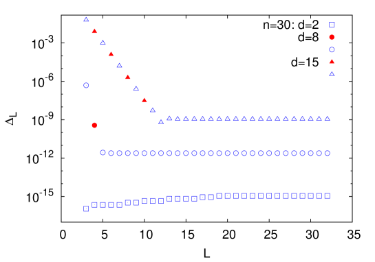
Refer to caption
Figure 10: Absolute value of ΔLsubscriptΔ𝐿\Delta_{L} in a chain of repulsive interactions. Filled and empty symbols show positive and negative values, respectively.

It is instructive here to compare the above hard sphere problem with a system of attractive interactions where the constraints Iij(σi,σj)subscript𝐼𝑖𝑗subscript𝜎𝑖subscript𝜎𝑗I_{ij}(\sigma_{i},\sigma_{j}) are satisfied if D(σi,σj)d𝐷subscript𝜎𝑖subscript𝜎𝑗𝑑D(\sigma_{i},\sigma_{j})\leq d. Figure 11 displays ΔLsubscriptΔ𝐿\Delta_{L} in a chain of attractive interactions; ΔLsubscriptΔ𝐿\Delta_{L} is positive for small L𝐿L but approaches an exponentially small negative value for large L𝐿L and d𝑑d. In this case, we expect to have asymptotically Δt0subscriptΔ𝑡0\Delta_{t}\geq 0. This is similar to the Griffiths inequalities G-jmath-1967 for ferromagnetic systems. Actually, using the Fortuin-Kasteleyn-Ginibre (FKG) inequalities FKG-cmath-1971 one can prove the above statement for soft attractive interactions, where Iij(σi,σj)=eβND(σi,σj)subscript𝐼𝑖𝑗subscript𝜎𝑖subscript𝜎𝑗superscript𝑒𝛽𝑁𝐷subscript𝜎𝑖subscript𝜎𝑗I_{ij}(\sigma_{i},\sigma_{j})=e^{-\frac{\beta}{N}D(\sigma_{i},\sigma_{j})} and β0𝛽0\beta\geq 0:

Refer to caption
Figure 11: Absolute value of ΔLsubscriptΔ𝐿\Delta_{L} in a chain of attractive interactions. Filled and empty symbols show positive and negative values, respectively.

Consider the following measure on configurations σ¯ΛN¯𝜎superscriptΛ𝑁\underline{\sigma}\in\Lambda^{N} where Λ={0,1}nΛsuperscript01𝑛\Lambda=\{0,1\}^{n},

μ(σ¯)etIe(σie,σje).proportional-to𝜇¯𝜎subscriptproduct𝑒subscript𝑡subscript𝐼𝑒subscript𝜎subscript𝑖𝑒subscript𝜎subscript𝑗𝑒\mu(\underline{\sigma})\propto\prod_{e\in\mathcal{E}_{t}}I_{e}(\sigma_{i_{e}},\sigma_{j_{e}}). (130)

This measure satisfies the conditions of the FKG inequality; ΛNsuperscriptΛ𝑁\Lambda^{N} is a partially ordered set and μ(σ¯)𝜇¯𝜎\mu(\underline{\sigma}) is convex, that is given two configurations σ¯¯𝜎\underline{\sigma} and σ¯superscript¯𝜎\underline{\sigma}^{\prime}

μ(σ¯max)μ(σ¯min)μ(σ¯)μ(σ¯),𝜇superscript¯𝜎𝑚𝑎𝑥𝜇superscript¯𝜎𝑚𝑖𝑛𝜇¯𝜎𝜇superscript¯𝜎\mu(\underline{\sigma}^{max})\mu(\underline{\sigma}^{min})\geq\mu(\underline{\sigma})\mu(\underline{\sigma}^{\prime}), (131)

where σ¯max=max(σ¯,σ¯)superscript¯𝜎𝑚𝑎𝑥¯𝜎superscript¯𝜎\underline{\sigma}^{max}=\max(\underline{\sigma},\underline{\sigma}^{\prime}) and σ¯min=min(σ¯,σ¯)superscript¯𝜎𝑚𝑖𝑛¯𝜎superscript¯𝜎\underline{\sigma}^{min}=\min(\underline{\sigma},\underline{\sigma}^{\prime}). These are bitwise max and min functions. One can use induction to show that D(σimax,σjmax)+D(σimin,σjmin)D(σi,σj)+D(σi,σj)𝐷superscriptsubscript𝜎𝑖𝑚𝑎𝑥superscriptsubscript𝜎𝑗𝑚𝑎𝑥𝐷superscriptsubscript𝜎𝑖𝑚𝑖𝑛superscriptsubscript𝜎𝑗𝑚𝑖𝑛𝐷subscript𝜎𝑖subscript𝜎𝑗𝐷superscriptsubscript𝜎𝑖superscriptsubscript𝜎𝑗D(\sigma_{i}^{max},\sigma_{j}^{max})+D(\sigma_{i}^{min},\sigma_{j}^{min})\leq D(\sigma_{i},\sigma_{j})+D(\sigma_{i}^{\prime},\sigma_{j}^{\prime}) which proves the convexity of μ(σ¯)𝜇¯𝜎\mu(\underline{\sigma}) for the soft attractive interactions.

Having these conditions the FKG inequality says that for decreasing (increasing) functions f(σ¯)𝑓¯𝜎f(\underline{\sigma}) and g(σ¯)𝑔¯𝜎g(\underline{\sigma})

fgfg0,delimited-⟨⟩𝑓𝑔delimited-⟨⟩𝑓delimited-⟨⟩𝑔0\langle fg\rangle-\langle f\rangle\langle g\rangle\geq 0, (132)

where the averages are taken with respect to the measure μ(σ¯)𝜇¯𝜎\mu(\underline{\sigma}). A function f(σ¯)𝑓¯𝜎f(\underline{\sigma}) is decreasing if f(σ¯)f(σ¯)𝑓¯𝜎𝑓superscript¯𝜎f(\underline{\sigma})\geq f(\underline{\sigma}^{\prime}) for any σ¯σ¯superscript¯𝜎¯𝜎\underline{\sigma}^{\prime}\geq\underline{\sigma}. The latter is a bit-wise inequality.

Now consider decreasing functions f=I[D(σi,0)li]𝑓𝐼delimited-[]𝐷subscript𝜎𝑖0subscript𝑙𝑖f=I[D(\sigma_{i},0)\leq l_{i}] and g=I[D(σj,0)lj]𝑔𝐼delimited-[]𝐷subscript𝜎𝑗0subscript𝑙𝑗g=I[D(\sigma_{j},0)\leq l_{j}] where 00 is the zero member of ΛΛ\Lambda. According to the FKG inequality we have

I[D(σi,0)0]I[D(σj,0)l]I[D(σi,0)0]I[D(σj,0)l],delimited-⟨⟩𝐼delimited-[]𝐷subscript𝜎𝑖00𝐼delimited-[]𝐷subscript𝜎𝑗0𝑙delimited-⟨⟩𝐼delimited-[]𝐷subscript𝜎𝑖00delimited-⟨⟩𝐼delimited-[]𝐷subscript𝜎𝑗0𝑙\langle I[D(\sigma_{i},0)\leq 0]I[D(\sigma_{j},0)\leq l]\rangle\geq\langle I[D(\sigma_{i},0)\leq 0]\rangle\langle I[D(\sigma_{j},0)\leq l]\rangle, (133)

which means Pt[D(σi,σj)l]P0[D(σi,σj)l]subscript𝑃𝑡delimited-[]𝐷subscript𝜎𝑖subscript𝜎𝑗𝑙subscript𝑃0delimited-[]𝐷subscript𝜎𝑖subscript𝜎𝑗𝑙P_{t}[D(\sigma_{i},\sigma_{j})\leq l]\geq P_{0}[D(\sigma_{i},\sigma_{j})\leq l] for any i,j,𝑖𝑗i,j, and l𝑙l. In other words, it is more likely to find two spheres closer to each other compared to the uniform measure. As a result, for the soft attractive interactions BP provides a lower bound for the log-partition function.

Actually for the soft interactions Iij(σi,σj)=e±βND(σi,σj)subscript𝐼𝑖𝑗subscript𝜎𝑖subscript𝜎𝑗superscript𝑒plus-or-minus𝛽𝑁𝐷subscript𝜎𝑖subscript𝜎𝑗I_{ij}(\sigma_{i},\sigma_{j})=e^{\pm\frac{\beta}{N}D(\sigma_{i},\sigma_{j})} the partition function reads

Z=σ¯e±βNi<jD(σi,σj)=[M=0N(NM)e±βM(1M/N)]n.𝑍subscript¯𝜎superscript𝑒plus-or-minus𝛽𝑁subscript𝑖𝑗𝐷subscript𝜎𝑖subscript𝜎𝑗superscriptdelimited-[]superscriptsubscript𝑀0𝑁𝑁𝑀superscript𝑒plus-or-minus𝛽𝑀1𝑀𝑁𝑛Z=\sum_{\underline{\sigma}}e^{\pm\frac{\beta}{N}\sum_{i<j}D(\sigma_{i},\sigma_{j})}=[\sum_{M=0}^{N}\left(\begin{array}[]{c}N\\ M\end{array}\right)e^{\pm\beta M(1-M/N)}]^{n}. (134)

One can exactly solve the problem in the thermodynamic limit and compare the results with the BP predictions to confirm the above statement for the attractive interactions. In the case of repulsive interactions the BP and exact results asymptotically coincide.

References

  • (1) S. Torquato, and F. H. Stillinger, Reviews of Modern Physics 82, 2633 (2010).
  • (2) G. Parisi, and F. Zamponi, Reviews of Modern Physics 82, 789 (2010).
  • (3) R. W. Hamming, Bell Syst. Tech. Jnl. 29, 147 (1950).
  • (4) E. N. Gilbert, Bell Syst. Tech. Jnl. 31, 504 (1952).
  • (5) R. R. Varshamov, Dokl. Akad. Nauk SSSR 117, 739 (1957).
  • (6) R. J. McEliece, E. R. Rodenmich, H. Rumsey, and L. R. Welch, IEEE Trans. Inform. Theory 23, 157 (1977).
  • (7) P. Delsarte and V. I. Levenshtein, IEEE Trans. Inform. Theory, 44(6), 2477 (1998).
  • (8) A. Barg and D. B. Jaffe, in ”Codes and Association Schemes” (A. Barg and S. Litsyn, Eds.), Amer. Math. Soc., Providence, (2001).
  • (9) A. Samorodnitsky, Journal of Combinatorial Theory, Series A 96, 261 (2001).
  • (10) T. Jiang and A. Vardy, IEEE Trans. Inform. Theory 50, 1655 (2004).
  • (11) A. Procacci and B. Scoppola, J. Stat. Phys. 96, 907 (1999).
  • (12) G. Parisi and F. Zamponi, J. Stat. Phys. 123, 1145 (2006).
  • (13) G. Parisi and F. Zamponi, J. Chem. Phys. 123, 144501 (2005).
  • (14) G. Parisi and F. Zamponi, J. Stat. Mech. (2006), P03017.
  • (15) M. Mézard and G. Parisi, Eur. Phys. J. B 20, 217 (2001).
  • (16) M. Mézard, G. Parisi, and R. Zecchina, Science 297, 812 (2002).
  • (17) M. Mézard and R. Zecchina, Phys. Rev. E 66, 056126 (2002).
  • (18) M. Mézard and G. Parisi, J. Stat. Phys. 111 (1-2), 1 (2003).
  • (19) M. Mezard, G. Parisi, and M. A. Virasoro, Spin-Glass Theory and Beyond, vol 9 of Lecture Notes in Physics (World Scientific, Singapore, 1987).
  • (20) M. Bailly-Bechet, C. Borgs, A. Braunstein, J. Chayes, A. Dagkessamanskaia, J-M Franois, and R. Zecchina, Proc. Natl. Acad. Sci. USA 108, 882 (2011).
  • (21) A. Braunstein, M. Mezard, and R. Zecchina, Random Structures and Algorithms 27, 201 (2005).
  • (22) F. Guerra, Commun. Math. Phys. 233, 1 (2003).
  • (23) S. Franz and M. Leone, J. Stat. Phys. 111(3-4), 535 (2003).
  • (24) S. Franz, M. Leone, and F. L. Toninelli, J. Phys. A: Math. Gen. 36, 10967 (2003).
  • (25) F. R. Kschischang, B. J. Frey, and H. -A. Loeliger, IEEE Trans. Infor. Theory 47, 498 (2001)
  • (26) F. Krzakala, A. Montanari, F. Ricci-Tersenghi, G. Semerjian, and L. Zdeborova, Proc. Natl. Acad. Sci. USA 104(25), 10318 (2007).
  • (27) M. J. A. Sloan, Amer. Math. Monthly 84, 82 (1977). See also the Table of Nonlinear Binary Codes at ”http://www2.research.att.com/ njas/codes/And/”.
  • (28) S. Torquato and F. H. Stillinger, Phys. Rev. E 73, 031106 (2006).
  • (29) S. Torquato and F. H. Stillinger, Experimental Mathematics 15, 307 (2006).
  • (30) S. Torquato, Random Heterogeneous Material: Microstructure and Macroscopic Properties, Springer-Verlag, New York (2002).
  • (31) A. Braunstein and R. Zecchina, Phys. Rev. Lett. 96, 030201 (2006).
  • (32) M. A. Tsfasman and S. G. Vladut, Algebraic-Geometric Codes, Kluwer, Dordrecht (1991).
  • (33) A. Montanari and F. Ricci-Tersenghi, Eur. Phys. J. B 33, 339 (2003).
  • (34) O. Rivoire, G. Biroli, O. C. Martin, and M. Mézard, Eur. Phys. J. B 37, 55 (2004).
  • (35) A. Montanari, G. Parisi, and F. Ricci-Tersenghi, J. Phys. A: Math. Gen. 37, 2073 (2004).
  • (36) R. B. Griffiths, J. Math. Phys. 8, 478-481 (1967).
  • (37) C. M. Fortuin, P. W. Kasteleyn, and J. Ginibre, Commun. Math. Phys. 22, 89 (1971).