Atom-atom correlations in time-of-flight imaging of ultra-cold bosons in optical lattices

Abstract

We study the spatial correlations of strongly interacting bosons in a ground state, confined in two-dimensional square and three-dimensional cubic lattice. Using combined Bogoliubov method and the quantum rotor approach, we map the Hamiltonian of strongly interacting bosons onto U(1) phase action in order to calculate the atom-atom correlations decay along the principal axis and a diagonal of the lattice plane direction as a function of distance. Lower tunneling rates lead to quicker decays of the correlations, which character becomes exponential. Finally, correlation functions allow us to calculate quantities that are directly bound to experimental outcomes, namely time-of-flight absorption images and resulting visibility. Our results contain all the characteristic features present in experimental data (transition from Mott insulating blob to superfluid peaks, etc.), which emphasizes the usability of the proposed approach.

I Introduction

During the last years enormous progress was made in the experimental study of cold atoms in optical lattices optical_lattices . The great advantage of optical lattices as analog simulators of strongly correlated Hamiltonians lies in the ability of optical lattices to accurately implement lattice models without impurities or defects. Furthermore, ultra-cold atoms confined in optical lattice structure provide a very clean experimental realization of a strongly correlated many-body problem quantum_many_body . Strong correlation effects, which imply enhanced quantum fluctuations, are playing an increasingly important role in recent experiments on dilute quantum gases strong_correlations . To underline the importance of correlations and fluctuations involved the studies of correlation functions are called for. One strategy for boosting the importance of correlations and fluctuations involves the study of the atomic correlators as a function of control of coupling parameters. The atom-atom correlation function is defined by:

$$C\left(\mathbf{r},\mathbf{r}^{\prime}\right)=\left\langle a\left(\mathbf{r}\right)a^{\dagger}\left(\mathbf{r}^{\prime}\right)\right\rangle,$$ (1)

where $a\left(\mathbf{r}\right)$ is a bosonic operator and $\left\langle\dots\right\rangle$ is statistical averaging translation_satement . This quantity is required for computing time-of-flight absorption images, as obtained with ultra-cold atoms released from optical lattices Gerbier ; Hoffman . We will calculate this quantity using the quantum rotor approach developed in our previous works polak1 ; zaleski1 , however now substantially supplemented by the implementation of the Bogoliubov method bogoliubov .

In experiment, one can envisage to measure the momentum distribution of the out-going atoms by taking a selective time of flight image (TOF). For homogeneous case, time of flight measurements probe the single-particle Green’s function at equal times i.e. the one-body density matrix. In an experiment of time-of-flight imaging, the cloud of ultra-cold atoms is first suddenly released from the harmonic trap. After a time of flight $t$, the position of the atoms is proportional to the momentum of the atoms in the initial cloud. Finally, an absorption image of the expanding cloud of atoms is taken by a probing laser. The resulting image provides directly the distribution of the momentum space $n(\mathbf{k})$. It is our goal of the presented paper to calculate the time-of-flight patterns using the combined Bogoliubov method and the quantum rotor approach and show that our approach recreates all the characteristic features that are observed in experimental settings. The plan of the paper is as follows: in Section II, we introduce the microscopic Bose-Hubbard model relevant for the description of strongly interacting bosons in an optical lattice. In the next Section, we perform the evaluation of the atom-atom correlation function by splitting the bosonic field into its amplitude and phase. Furthermore, in Section III, by implementing the Bogoliubov method to the amplitude part of the bosonic field and combining its outcome with the quantum rotor approach, we derive analytically the explicit expressions for the atom-atom correlation function, time-of-flight absorption images and visibility. In Section IV, results of our calculations are plotted: the spatial dependence of the correlation function as a function of lattice distance $\mathbf{R}$, time-of-flight images and visibility for various model parameters. Finally, we conclude in the Section V.

II Model Hamiltonian

From a theoretical point of view, description of the bosons in optical lattice can be achieved through the definition of a microscopic Hamiltonian, which can capture the main physics of these systems: the Bose Hubbard Hamiltonian. Within this model, the bosons move on a lattice within a tight-binding scheme and correlation is introduced through an on-site repulsive term, since in real Bose gases the interaction between atoms cannot be neglected in the physical description of the gas. We consider a second quantized, bosonic Hubbard Hamiltonian in the form bemodel1 ; bemodel2 :

$$\mathcal{H} = -t\sum_{\left\langle\mathbf{r},\mathbf{r}^{\prime}\right\rangle}\left[a^{\dagger}\left(\mathbf{r}\right)a\left(\mathbf{r}^{\prime}\right)+a^{\dagger}\left(\mathbf{r}^{\prime}\right)a\left(\mathbf{r}\right)\right]$$ (2)

$$+\frac{U}{2}\sum_{\mathbf{r}}n^{2}\left(\mathbf{r}\right)-\overline{\mu}\sum_{\mathbf{r}}n\left(\mathbf{r}\right).$$

The constant $t$ represents nearest neighbors tunneling matrix element and is responsible for the dynamical hopping of bosons from one optical lattice site to another. During a jump between two neighboring sites a boson gains energy $t$. The constant $U$ is the strength of the on-site repulsive interaction of bosons. Adding a boson to already occupied site costs energy $U$. Furthermore, $\overline{\mu}=\mu+\frac{U}{2}$, where $\mu$ is a chemical potential controlling the average number of bosons. The operators $a^{\dagger}\left(\mathbf{r}\right)$ and $a\left(\mathbf{r}^{\prime}\right)$ create and annihilate bosons on sites $\mathbf{r}$ and $\mathbf{r}^{\prime}$ of a regular two-dimensional (2D) lattice with the nearest neighbors hopping denoted by summation over $\left\langle\mathbf{r},\mathbf{r}^{\prime}\right\rangle$. A total number of sites is equal to $N$ and the boson number operator $n\left(\mathbf{r}\right)=a^{\dagger}\left(\mathbf{r}\right)a\left(\mathbf{r}\right)$. We use the Hamiltonian in Eq. (2) to describe a homogeneous (translationally invariant) system, omitting the effect of the external magnetic potential that is usually superimposed on top of the optical lattice potential in order to additionally trap the atoms. The external potential can be included in the Hamiltonian as $\sum_{\mathbf{r}}\epsilon\left(\mathbf{r}\right)n\left(\mathbf{r}\right)$ and would couple to the chemical potential term. We discuss such a scenario and its consequences in the Section IV. The realization of the Bose-Hubbard Hamiltonian using optical lattices has the advantage that the interaction matrix element $U$ and the tunneling matrix element $t$ can be controlled by adjusting the intensity of the laser beams. The Hamiltonian and its descendants have been widely studied within the last years. The phase diagram and ground-state properties include the mean-field ansatz key-1 , strong coupling expansions key-2 ; key-3 ; key-4 , the quantum rotor approach key-5 , methods using the density matrix renormalization group DMRG key-6 ; key-7 ; key-8 ; key-9 , and quantum Monte Carlo QMC simulations key-10 ; key-11 ; key-12 ; key-13 .

III Atomic correlation functions

III.1 Transformation to the amplitude-phase variables

The statistical sum of the system defined by Eq. (2) can be written in a path integral form with use of complex fields, $a\left(\mathbf{r}\tau\right)$ depending on the “imaginary time” $0\leq\tau\leq\beta\equiv 1/k_{B}T$, (with $T$ being the temperature) that satisfy the periodic condition $a\left(\mathbf{r}\tau\right)=a(\mathbf{r}\tau+\beta)$:

$$Z=\int\left[\mathcal{D}\overline{a}\mathcal{D}a\right]e^{-\mathcal{S}\left[\overline{a},a\right]},$$ (3)

where the action $\mathcal{S}$ is equal to:

$$\mathcal{S}\left[\overline{a},a\right]=\int_{0}^{\beta}d\tau\left[\mathcal{H}\left(\tau\right)+\sum_{\mathbf{r}}\overline{a}\left(\mathbf{r}\tau\right)\frac{\partial}{\partial\tau}a\left(\mathbf{r}\tau\right)\right].$$ (4)

Now, we are briefly introducing the quantum rotor approach, which has already been employed for the calculation of the phase diagram of the cold bosons in optical lattice polak1 . The fourth-order term in the Hamiltonian in Eq. (2) can be decoupled using the Hubbard-Stratonovich transformation with an auxiliary field $V\left(\mathbf{r}\tau\right)$:

$$e^{-\frac{U}{2}\sum_{\mathbf{r}}\int_{0}^{\beta}d\tau n^{2}\left(\mathbf{r}\tau\right)}$$

$$\,\,\,\,\,\propto\int\frac{\mathcal{D}V}{\sqrt{2\pi}}e^{\sum_{\mathbf{r}}\int_{0}^{\beta}d\tau\left[-\frac{V^{2}\left(\mathbf{r}\tau\right)}{2U}+iV\left(\mathbf{r}\tau\right)n\left(\mathbf{r}\tau\right)\right]}.$$ (5)

The fluctuating “imaginary chemical potential” $iV\left(\mathbf{r}\tau\right)$ can be written as a sum of static $V^{\circ}\left(\mathbf{r}\right)$ and periodic function:

$$V\left(\mathbf{r}\tau\right) = V^{\circ}\left(\mathbf{r}\right)+\tilde{V}\left(\mathbf{r}\tau\right),$$ (6)

where, using Fourier series:

$$\tilde{V}\left(\mathbf{r}\tau\right) = \frac{1}{\beta}\sum_{\ell=1}^{\infty}\tilde{V}\left(\mathbf{r}\omega_{\ell}\right)\left(e^{i\omega_{\ell}\tau}+e^{-i\omega_{\ell}\tau}\right),$$ (7)

with the Bose-Matsubara frequencies are $\omega_{\ell}=2\pi\ell/\beta$ and $\ell=0,\pm 1,\pm 2,\dots$. Introducing the U(1) phase field $\phi\left(\mathbf{r}\tau\right)$ via the Josephson-type relation kopec1 :

$$\dot{\phi}\left(\mathbf{r}\tau\right)=\tilde{V}\left(\mathbf{r}\tau\right)$$ (8)

with $\dot{\phi}\left(\mathbf{r}\tau\right)=\partial\phi\left(\mathbf{r}\tau\right)/\partial\tau$ we can now perform a local gauge transformation to new bosonic variables:

$$a\left(\mathbf{r}\tau\right)=b\left(\mathbf{r}\tau\right)e^{i\phi\left(\mathbf{r}\tau\right)}.$$ (9)

As a result, the strongly correlated bosonic system is transformed into a weakly interacting bosons, submerged into the bath of strongly fluctuating gauge potentials (which interactions are governed by the high energy scale of $U$). The order parameter is defined by:

$${\bf\Psi}_{B}=\left\langle a\left(\mathbf{r}\tau\right)\right\rangle=\left\langle b\left(\mathbf{r}\tau\right)\right\rangle\psi_{B}.$$ (10)

However, one should note that a nonzero value of the amplitude $\left\langle b\left(\mathbf{r}\tau\right)\right\rangle$ is not sufficient for superfluidity. To achieve this, also the phase (rotor) variables, must become stiff and coherent. The phase order parameter is defined by:

$$\psi_{B}=\left\langle e^{i\phi\left(\mathbf{r}\tau\right)}\right\rangle_{\phi},$$ (11)

where $\left\langle\dots\right\rangle_{\phi}$ is averaging over phase action to be calculated in the next subsection. This reflects the fact that all the atoms in the condensate have the same phase and form a coherent matter wave. Thus the condensate possess a well defined phase associated with the concept of so-called spontaneously broken U(1) gauge symmetry.

After the variable transformations the statistical sum becomes:

$$Z=\int\left[\mathcal{D}\bar{b}\mathcal{D}b\right]\left[\mathcal{D}\phi\right]e^{-\mathcal{S}\left[\bar{b},b,\phi\right]}$$ (12)

with the action:

$$\mathcal{S}\left[\overline{b},b,\phi\right]=\sum_{\mathbf{r}}\int_{0}^{\beta}d\tau\overline{b}\left(\mathbf{r}\tau\right)\frac{\partial}{\partial\tau}b\left(\mathbf{r}\tau\right)$$

$$-t\sum_{\left\langle\mathbf{r},\mathbf{r}^{\prime}\right\rangle}\int_{0}^{\beta}d\tau\left\{e^{-i\left[\phi\left(\mathbf{r}\tau\right)-\phi\left(\mathbf{r}^{\prime}\tau\right)\right]}\overline{b}\left(\mathbf{r}\tau\right)b\left(\mathbf{r}^{\prime}\tau\right)+h.c.\right\}$$

$$+\sum_{\mathbf{r}}\int_{0}^{\beta}d\tau\left[U\left\langle\overline{b}\left(\mathbf{r}\tau\right)b\left(\mathbf{r}\tau\right)\right\rangle_{b}-\overline{\mu}\right]\overline{b}\left(\mathbf{r}\tau\right)b\left(\mathbf{r}\tau\right)$$

$$+\sum_{\mathbf{r}}\int_{0}^{\beta}d\tau\left[\frac{1}{2U}\dot{\phi}^{2}\left(\mathbf{r}\tau\right)+i\frac{\overline{\mu}}{U}\dot{\phi}\left(\mathbf{r}\tau\right)\right],$$ (13)

which will be used as a departure point for obtaining bosonic and phase-only actions.

III.2 Transformation to the rotor representation for phase variables

The statistical sum can be integrated over the phase or bosonic variables with the phase or bosonic action:

$$\mathcal{S}_{\phi}\left[\phi\right] = -\ln\int\left[\mathcal{D}\bar{b}\mathcal{D}b\right]e^{-\mathcal{S}\left[\bar{b},b,\phi\right]},$$

$$\mathcal{S}_{b}\left[\overline{b},b\right] = -\ln\int\left[\mathcal{D}\phi\right]e^{-\mathcal{S}\left[\bar{b},b,\phi\right]}$$ (14)

to obtain:

$$Z=\int\left[\mathcal{D}\phi\right]e^{-\mathcal{S}_{\phi}\left[\phi\right]}=\int\left[\mathcal{D}\overline{b}\mathcal{D}b\right]e^{-\mathcal{S}_{b}\left[\overline{b},b\right]}.$$ (15)

In order to calculate the phase-only action, we use the following approximation:

$$a\left(\mathbf{r}\tau\right)=b\left(\mathbf{r}\tau\right)e^{i\phi\left(\mathbf{r}\tau\right)}\approx b_{0}e^{i\phi\left(\mathbf{r}\tau\right)},$$ (16)

where $b_{0}$ is static bosonic amplitude, which will be calculated in the next Section. The phase-only action from Eq. (14) can be written explicitly:

$$\mathcal{S}_{\phi}\left[\phi\right] = \int_{0}^{\beta}d\tau\left\{\sum_{\mathbf{r}}\left[\frac{\dot{\phi}^{2}\left(\mathbf{r}\tau\right)}{2U}+i\frac{\overline{\mu}}{U}\dot{\phi}\left(\mathbf{r}\tau\right)\right]\right.$$ (17)

$$- \left.J\sum_{\left\langle\mathbf{r},\mathbf{r}^{\prime}\right\rangle}\cos\left[\phi\left(\mathbf{r}\tau\right)-\phi\left(\mathbf{r}^{\prime}\tau\right)\right]\right\},$$

where $J=t\left|b_{0}\right|^{2}$ represents the stiffness for the phase field. It is clear that the phase action is non-linear in the phase variables $\phi\left(\mathbf{r}\tau\right)$ and the statistical sum in Eq. (15) cannot be calculated exactly. Because of the trigonometric nature of the phase variables it is useful to introduce a new uni-modular collective field $z\left(\mathbf{r}\tau\right)=e^{i\phi\left(\mathbf{r}\tau\right)}$, which will be treated within the quantum rotor approach by making use of the following resolution of unity:

$$1\equiv\int d\overline{z}dz\delta\left[z\left(\mathbf{r}\tau\right)-e^{i\phi\left(\mathbf{r}\tau\right)}\right]\delta\left[\overline{z}\left(\mathbf{r}\tau\right)-e^{-i\phi\left(\mathbf{r}\tau\right)}\right].$$ (18)

The unit length constraint for $z\left(\mathbf{r}\tau\right)$ variables is implemented on average by the formula (see, Ref. kopec2, ):

$$\delta\left[N-\sum_{\mathbf{r}}\overline{z}\left(\mathbf{r}\tau\right)z\left(\mathbf{r}\tau\right)\right]=\int d\lambda e^{N\lambda-\lambda\sum_{\mathbf{r}}\overline{z}\left(\mathbf{r}\tau\right)z\left(\mathbf{r}\tau\right)},$$ (19)

which introduces a Lagrange multiplier $\lambda$. Substituting Eq. (18) into Eq. (15) and integrating by the cumulant expansion over the phase variables, the partition function reads:

$$Z = \int\left[\mathcal{D}\overline{z}\mathcal{D}z\right]d\lambda e^{N\lambda-\mathcal{S}_{z}\left[\overline{z},z\right]},$$ (20)

In the thermodynamic limit ($N\rightarrow\infty$), the integral (20) can be performed exactly by the saddle-point method. The quantum rotor action:

$$\mathcal{S}_{z}\left[\overline{z},z\right] = \sum_{\left\langle\mathbf{r},\mathbf{r}^{\prime}\right\rangle}\int_{0}^{\beta}d\tau d\tau^{\prime}\left[\left(\lambda\delta_{\mathbf{r}\mathbf{r}^{\prime}}-tb_{0}^{2}\right)\delta\left(\tau-\tau^{\prime}\right)\right.$$ (21)

$$\left.+\delta_{\mathbf{r}\mathbf{r}^{\prime}}K^{-1}\left(\tau-\tau^{\prime}\right)\right]\overline{z}\left(\mathbf{r}\tau\right)z\left(\mathbf{r}^{\prime}\tau^{\prime}\right),$$

where $K^{-1}\left(\tau-\tau^{\prime}\right)$ is a phase correlator, which includes dynamic effect of the U(1) phase field:

$$K^{-1}\left(\tau-\tau^{\prime}\right)=\left\langle e^{i\phi\left(\mathbf{r}\tau\right)-i\phi\left(\mathbf{r}\tau^{\prime}\right)}\right\rangle_{0}.$$ (22)

Furthermore, the average

$$\left\langle\dots\right\rangle_{0}=\frac{\int\left[\mathcal{D}\phi\right]\dots e^{-\mathcal{S}_{0}\left[\phi\right]}}{\int\left[\mathcal{D}\phi\right]e^{-\mathcal{S}_{0}\left[\phi\right]}}$$ (23)

is taken only over non-interacting quantum rotors:

$$\mathcal{S}_{0}=\sum_{\mathbf{r}}\int_{0}^{\beta}d\tau\left[\frac{\dot{\phi}^{2}\left(\mathbf{r}\tau\right)}{2U}+i\frac{\overline{\mu}}{U}\dot{\phi}\left(\mathbf{r}\tau\right)\right].$$ (24)

The Fourier transform of the correlator in Eq. (22) in zero temperature limit reads:

$$K^{-1}\left(\omega_{\ell}\right)=\frac{U}{4}-U\left[v\left(\frac{\overline{\mu}}{U}\right)+\frac{i\omega_{\ell}}{U}\right]^{2},$$ (25)

where $v\left(x\right)=x-\left[x\right]-\frac{1}{2}$, and $\left[x\right]$ is the floor function, which gives the greatest integer less then or equal to $x$. Non-zero value of the order parameter $\Psi_{B}$ signals a bosonic condensation that we identify as superfluid state. The phase order parameter in the quantum rotor model can be written as:

$$1-\psi_{B}^{2}=\frac{1}{N}\sum_{\mathbf{r}}\int_{0}^{\beta}d\tau\left\langle\overline{z}\left(\mathbf{r}\tau\right)z\left(\mathbf{r}\tau\right)\right\rangle$$ (26)

which fixes value of the phase order parameter $\psi_{B}$. The Lagrange multiplier saddle-point value “sticks” at criticality to the value $\lambda_{0}$ given by

$$\lambda_{0}-J\left(\mathbf{k}=0\right)+K^{-1}\left(\omega_{\ell=0}\right)=0,$$ (27)

and obeys the Eq. (27) in the whole low temperature ordered phase.

III.3 Bogoliubov transformation of the amplitude bosonic variables

In the Bogoliubov approximation the complicated many-body quartic Hamiltonian is reduced to a quadratic one, which can be diagonalized exactly. In order to calculate the bosonic action in Eq. (14), we follow the Bogoliubov approach by splitting the bosonic operator into a Bose condensate macroscopic occupation $N_{0}=b_{0}^{2}$ and non-condensed fluctuation part $b_{d}\left(\mathbf{r}\right)$ bogoliubov . As a consequence, the original operator splits into a sum and according to Eq. (9) at an alternative representation:

$$b\left(\mathbf{r}\tau\right)=b_{0}+b_{d}\left(\mathbf{r}\tau\right).$$ (28)

Substituting the Eq. (28) into the action in Eq. (14), and neglecting the terms of the order higher than two in $b_{d}\left(\mathbf{r}\right)$ operators, the action reads:

$$\mathcal{S}=\mathcal{S}_{0}+\mathcal{S}_{1}+\mathcal{S}_{2},$$ (29)

where the zero, first and the second order terms containing interactions within and between both sub-systems are:

$$\mathcal{S}_{0} = N\beta\left[-tz-\overline{\mu}+\frac{U}{2}\left|b_{0}\right|^{2}\right]\overline{b}_{0}b_{0}.$$ (30)

The linear part in the fluctuation operators reads:

$$\mathcal{S}_{1}=\sum_{\mathbf{r}}\int_{0}^{\beta}d\tau\left\{\left[-zt-\overline{\mu}+U\left|b_{0}\right|^{2}\right]\overline{b}_{0}b_{d}\left(\mathbf{r}\tau\right)\right\}$$

$$+\sum_{\mathbf{r}}\int_{0}^{\beta}d\tau\left\{\left[-zt-\overline{\mu}+U\left|b_{0}\right|^{2}\right]b_{0}\overline{b}_{d}\left(\mathbf{r}\tau\right)\right\},$$ (31)

and finally, the quadratic part:

$$\mathcal{S}_{2}=\frac{1}{2}\sum_{\mathbf{r}}\int_{0}^{\beta}d\tau d\tau^{\prime}\,\left[\begin{array}[]{cc}\overline{b}_{d}\left(\mathbf{r}\tau\right),&b_{d}\left(\mathbf{r}\tau^{\prime}\right)\end{array}\right]$$ (33)

$$\times\left[\begin{array}[]{cc}2U\left|b_{0}\right|^{2}-A_{+}&U\left|b_{0}\right|^{2}\\ U\left|b_{0}\right|^{2}&2U\left|b_{0}\right|^{2}-A_{-}\end{array}\right]\left[\begin{array}[]{c}b_{d}\left(\mathbf{r}\tau\right)\\ \overline{b}_{d}\left(\mathbf{r}\tau^{\prime}\right)\end{array}\right]$$ (38)

$$-t\sum_{\left\langle\mathbf{r}>\mathbf{r}^{\prime}\right\rangle}\int_{0}^{\beta}d\tau\,\left[\overline{b}_{d}\left(\mathbf{r}\tau\right)b_{d}\left(\mathbf{r}^{\prime}\tau\right)+h.c.\right],$$ (39)

where:

$$A_{\pm}\left(\tau-\tau^{\prime}\right)=\overline{\mu}\mp\delta\left(\tau-\tau^{\prime}\right)\frac{\partial}{\partial\tau}.$$ (40)

Furthermore, the value of $b_{0}$ amplitude can be calculated in the saddle point:

$$\frac{\partial\mathcal{S}\left[b_{0}\right]}{\partial b_{0}}=-tz-\overline{\mu}+U\left|b_{0}\right|^{2}=0,$$ (41)

which results in:

$$\left|b_{0}\right|^{2}=z\frac{t}{U}+\frac{\overline{\mu}}{U}.$$ (42)

This implies that the linear term in Eq. (29) is $\mathcal{S}_{1}=0$ and the bosonic action is given by:

$$\mathcal{S}\left[\overline{b},b\right]=\mathcal{S}_{0}+\mathcal{S}_{2}.$$ (43)

III.4 Correlation function

Summarizing up the results of the preceding sections, the correlation function in Eq. (1) can be written as a product of two correlation functions of amplitude and rotor fields:

$$C\left(\mathbf{R}\right) \equiv C_{z}\left(\mathbf{R}\right)C_{b}\left(\mathbf{R}\right),$$ (44)

where

$$C_{z}\left(\mathbf{R}\right) \equiv C_{z}\left(\mathbf{r}\tau;\mathbf{r}^{\prime}\tau\right)=\left\langle z\left(\mathbf{r}\tau\right)\overline{z}\left(\mathbf{r}^{\prime}\tau\right)\right\rangle_{z}$$

$$C_{b}\left(\mathbf{R}\right) \equiv C_{b}\left(\mathbf{r}\tau;\mathbf{r}^{\prime}\tau\right)=\left\langle b\left(\mathbf{r}\right)\overline{b}\left(\mathbf{r}^{\prime}\right)\right\rangle_{b}.$$ (45)

The averagings appearing in Eq. (45) are defined by:

$$\left\langle\dots\right\rangle_{z} = \frac{\int\left[\mathcal{D}\overline{z}\mathcal{D}z\right]\dots e^{-\mathcal{S}_{z}\left[\overline{z},z\right]}}{\int\left[\mathcal{D}\overline{z}\mathcal{D}z\right]e^{-\mathcal{S}_{z}\left[\overline{z},z\right]}}$$

$$\left\langle\dots\right\rangle_{b} = \frac{\int\left[\mathcal{D}\bar{b}\mathcal{D}b\right]\dots e^{-\mathcal{S}_{b}\left[\overline{b},b\right]}}{\int\left[\mathcal{D}\bar{b}\mathcal{D}b\right]e^{-\mathcal{S}_{b}\left[\overline{b},b\right]}},$$ (46)

where $\mathcal{S}_{z}\left[\overline{z},z\right]$ and $\mathcal{S}_{b}\left[\overline{b},b\right]$ are given in Eqs. (21) and (43), respectively. As a result, the correlation function in the real space splits into a product of averages from bosonic and phase sectors. The Green’s function in the bosonic sector reads:

$$G_{b}\left(\mathbf{k}\omega_{m}\right)=b_{0}^{2}+G_{bd}^{22}\left(\mathbf{k}\omega_{m}\right),$$ (47)

where:

$$G_{bd}\left(\mathbf{k}\omega_{m}\right)$$

$$=\left[\begin{array}[]{cc}\frac{2t\left(\varepsilon_{\mathbf{0}}-\varepsilon_{\mathbf{k}}\right)+U\left|b_{0}\right|^{2}-i\omega_{\ell}}{E_{\mathbf{k}}^{2}-\left(i\omega_{\ell}\right)^{2}}&-\frac{U\left|b_{0}\right|^{2}}{E_{\mathbf{k}}^{2}-\left(i\omega_{\ell}\right)^{2}}\\ -\frac{U\left|b_{0}\right|^{2}}{E_{\mathbf{k}}^{2}-\left(i\omega_{\ell}\right)^{2}}&\frac{2t\left(\varepsilon_{\mathbf{0}}-\varepsilon_{\mathbf{k}}\right)+U\left|b_{0}\right|^{2}+i\omega_{\ell}}{E_{\mathbf{k}}^{2}-\left(i\omega_{\ell}\right)^{2}}\end{array}\right],\,\,\,\,\,\,\,\,\,\,$$ (50)

and

$$E_{\mathbf{k}}=\sqrt{2t\left(\frac{z}{2}-\varepsilon_{\mathbf{k}}\right)\left[2t\left(\frac{z}{2}-\varepsilon_{\mathbf{k}}\right)+2U\left|b_{0}\right|^{2}\right]}$$ (51)

with a dispersion for a simple cubic lattice:

$$\varepsilon_{\mathbf{k}}=\cos\left(ak_{x}\right)+\cos\left(ak_{y}\right)+\cos\left(ak_{z}\right).$$ (52)

On the other hand, the phase sector leads to the phase Green’s function:

$$G_{\phi}\left(\mathbf{k}\omega_{m}\right) = \left\langle z\left(\mathbf{k}\omega_{m}\right)\overline{z}\left(\mathbf{k}\omega_{m}\right)\right\rangle$$ (53)

$$= \frac{1}{\lambda_{0}-2tb_{0}^{2}\varepsilon_{\mathbf{k}}+K^{-1}\left(\omega_{m}\right)}.$$

As a result, the correlation function finally reads:

$$C\left(\mathbf{R}\right)=G_{\phi}\left(\mathbf{R}\right)\left[\left|b_{0}\right|^{2}+G_{bd}\left(\mathbf{R}\right)\right].$$ (54)

III.5 Spatial dependence of the correlation functions

The correlation function in Eq. (1) can be calculated along the lattice axis ($x$ or $y$), or along the diagonal of the square lattice:

$$\mathbf{R}_{\mathrm{parallel}} = \left(na_{x},0\right),$$

$$\mathbf{R}_{\mathrm{diagonal}} = \left(na_{x},na_{y}\right),$$ (55)

where $a_{x}$, and $a_{y}$ are lattice constants in $x$, and $y$ direction, respectively and $n$ is an integer. The results for two-dimensional square lattice are presented in Figs. 1a and b for the Mott state within the first and the fifth Mott lobe, respectively. The correlation function is plotted in logarithmic scale. As expected, lower tunneling rates lead to quicker decays of the correlations. Also, the character of the decay becomes exponential as on-site repulsion $U$ gets stronger (dependence becomes linear in logarithmic scale). Correlations calculated along the lattice diagonal are weaker than those parallel to the lattice axis (see, Fig. 1c), which is also in agreement with results from Ref. correlations, ).

From this result, we can deduce that the asymptotic spatial behavior of the correlation function $C\left(\mathbf{R}\right)$ is given by the formula:

$$C\left(\mathbf{R}\right)=\exp\left(-\frac{\left|\mathbf{R}\right|}{\xi}\right),$$ (56)

where $\xi$ stands for the correlation length. On the other hand, from Eq. (54) we see that the critical behavior (associated with ordering of the phase variables) is governed by $G_{\phi}\left(\mathbf{R}\right)$ [see, Eq. (53)] – a correlation function of the quantum spherical model criticalexponents , for which a universal quantum-critical ($T=0$) properties imply that the correlation length as a function of on-site scattering $U$, close to the critical point, should behave as:

$$\xi=\left(\frac{U-U_{c}}{U_{c}}\right)^{-1},$$ (57)

where $U_{c}$ is the critical value of $U$.

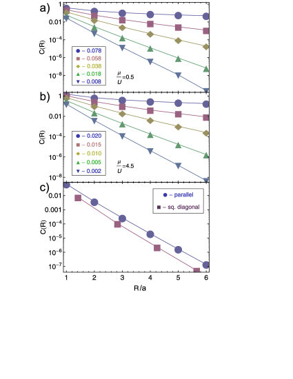
Figure 1: (Color online) Correlation function $C\left(\mathbf{R}\right)$ along axis direction for various values of $\frac{t}{U}$ for two-dimensional lattice inside a) the first and b) the fifth Mott lobe; c) comparison of correlations decay for $\frac{t}{U}=0.02$ and $\frac{\mu}{U}=0.5$ along axis (circles) and lattice in-plane diagonal (squares) for two-dimensional lattice.

IV Time-of-flight patterns

The phase coherence properties can be estimated from time of flight images. When atoms in the superfluid state are released from the trap and optical lattice, phase coherence leads to an interference pattern with interference peaks arranged in the order reflecting the optical lattice symmetry. However, the Mott insulating phase does not have long range phase coherence and does not show the interference pattern in the time-of-flight images. To identify the ordered state, we concentrate on the momentum distribution of particle number $n\left(\mathbf{k}\right)$, a quantity of basic interest that encodes the strong correlations of the system:

$$n\left(\mathbf{k}\right)=\sum_{\mathbf{R}}C\left(\mathbf{R}\right)e^{i\mathbf{k}\mathbf{R}}.$$ (58)

This quantity is measured in time-of-flight experiments, which are performed by releasing the atomic cloud from the optical trap potential. Due to the fact that the expansion is mainly ballistic, the momentum dependence of particle numbers represents the interference pattern, which typically has two distinct types of behavior: a wide maximum signifying the Mott insulating incoherent state, and a sharp peaks located in the reciprocal lattice vectors, which are considered as a signature of superfluidity in the system. According to the formulas in Eqs. (44)-(53), we have:

$$n\left(\mathbf{k}\right) = \left\langle a_{\mathbf{k}}^{\dagger}\left(\tau\right)a_{\mathbf{k}}\left(\tau\right)\right\rangle$$ (59)

$$= m_{0}\frac{1}{\beta}\sum_{m}G_{bd}\left(\mathbf{k}\omega_{m}\right)+b_{0}\frac{1}{\beta}\sum_{m}G_{\phi d}\left(\mathbf{k}\omega_{m}\right)$$

$$\,\,\,\,+\frac{1}{N\beta^{2}}\sum_{\mathbf{k}^{\prime},m,m^{\prime}}G_{bd}\left(\mathbf{k}^{\prime}\omega_{m}\right)G_{\phi d}\left(\mathbf{k}-\mathbf{k}^{\prime};\omega_{m^{\prime}}\right)$$

$$= m_{0}G_{bd}\left(\mathbf{k}\right)+b_{0}G_{\phi d}\left(\mathbf{k}\right)$$

$$\,\,\,\,+\frac{1}{N}\sum_{\mathbf{k}^{\prime}}G_{bd}\left(\mathbf{k}^{\prime}\right)G_{\phi d}\left(\mathbf{k}-\mathbf{k}^{\prime}\right),$$

where:

$$G_{bd}\left(\mathbf{k}\right) = \frac{1}{2}\left[-1+\frac{2t\left(\varepsilon_{0}-\varepsilon_{\mathbf{k}}\right)+n_{0}U}{E_{\mathbf{k}}}\coth\frac{\beta E_{\mathbf{k}}}{2}\right]$$

$$G_{\phi d}\left(\mathbf{k}\right) = \frac{\coth\left\{\frac{\beta U}{2}\left[\Omega_{\mathbf{k}}+v\left(\frac{\overline{\mu}}{U}\right)\right]\right\}}{4\Omega_{\mathbf{k}}}$$ (60)

$$+ \frac{\coth\left\{\frac{\beta U}{2}\left[\Omega_{\mathbf{k}}-v\left(\frac{\overline{\mu}}{U}\right)\right]\right\}}{4\Omega_{\mathbf{k}}},$$

with:

$$\Omega_{\mathbf{k}}=\sqrt{2\frac{tb_{0}^{2}}{U}\left(\varepsilon_{0}-\varepsilon_{\mathbf{k}}\right)+v^{2}\left(\frac{\overline{\mu}}{U}\right)+\frac{\delta\lambda}{U}}.$$ (61)

We now turn to the description of the interference pattern observed after release of the atom cloud from the optical lattice and a period of free expansion, where the phase coherence of the atoms on the optical lattice can be directly probed. The density distribution of the expanding cloud after time $t$ can be represented as follows tof1 ; tof2 ; tof3 :

$$n\left(\mathbf{r}\right)=\left.\left(\frac{m}{\hbar t}\right)^{3}\left|W\left(\mathbf{k}\right)\right|^{2}n\left(\mathbf{k}\right)\right|_{\mathbf{k}=\frac{m\mathbf{r}}{\hbar t}},$$ (62)

where $m$ is the atomic mass and $t$ is cloud expansion time. The quantity $W\left(\mathbf{k}\right)$ in the Eq. 62 is the Fourier transform of the Wannier function in the lowest Bloch band. Typically, the trapping potential is well approximated by a harmonic function so that the envelope has the Gaussian form:

$$\left|W\left(\frac{m\mathbf{r}}{\hbar t}\right)\right|^{2}\approx\frac{1}{\pi^{3/2}w_{t}}\exp\left(-\frac{\mathbf{r}^{2}}{w_{t}^{2}}\right),$$ (63)

where $w_{t}=\hbar t/mw_{0}$ with $w_{0}$ being the size of the on-site Wannier function. Therefore, in order to compare the interference pattern with experiments, we have to calculate $n\left(\mathbf{r}\right)$. However, the experimental absorption pictures are two-dimensional projections of the three-dimensional optical lattice, i.e. they are column-integrated momentum distribution over one axis:

$$n_{\perp}\left(k_{x},k_{y}\right)=\int dk_{z}\left|W\left(\mathbf{k}\right)\right|^{2}n\left(\mathbf{k}\right).$$ (64)

Observing that $n\left(\mathbf{k}\right)=n\left[G_{xd}\left(\mathbf{k}\right)\right]$, where $x$=$\phi,b$ (see, Eq. 59) and making an expansion:

$$G_{xd}\left(\mathbf{k}\right)=g_{0x}+g_{x}\varepsilon\left(\mathbf{k}\right)+O\left[\varepsilon\left(\mathbf{k}\right)\right],$$ (65)

where $\varepsilon\left(\mathbf{k}\right)$ is given by Eq. (52), we see that the contribution:

$$\int dk_{z}\left|W\left(\mathbf{k}\right)\right|^{2}\cos ak_{z}=\sqrt{\pi}w_{0}e^{-\left(\frac{aw_{0}}{2}\right)^{2}}\approx 0$$ (66)

is negligible for sufficiently large optical lattice depths, especially deep in the Mott regime. Thus, we can consider an effective two-dimensional system a good approximation of the three-dimensional one. The result is presented in Fig. 2. In the superfluid phase, the sharp peaks emerge denoting long-range phase coherence. In the Mott phase, the momentum distribution becomes a broad, featureless maximum.

To asses the interference pattern, a useful quantity is often introduced, which is called visibility and measured in many experiments vis1 ; vis2 ; vis3 :

$$v=\frac{n_{max}-n_{min}}{n_{max}+n_{min}}.$$ (67)

The minimum and maximum intensities $n_{min}$ and $n_{max}$ are measured at the same distance from the cloud center, which for two-dimensional square lattice are at $\mathbf{k}=\left(2\pi/\sqrt{2}a,2\pi/\sqrt{2}a\right)$ and $\mathbf{k}=\left(2\pi/a,0\right)$, respectively, at which the Wannier envelope in Eq. (63) cancels out. The resulting dependence of visibility on interaction ratio is presented in Fig. 3. In the superfluid phase, its value is almost 1 signaling strong coherence peaks in time-of-flight patters. Deeper within Mott lobes, the visibility is decreasing, while the time-of-flight pattern becomes a circularly symmetric blob. However, in Fig. 2 the phase transition occurs abruptly and signature of superfluidity, namely sharp peaks, disappear fast within the Mott phase. This is not usually observed in experiments, where the remainders of the peaks are visible even for systems deep in the Mott phase. It results from the fact that in the experimental setups the atoms are trapped not only within the optical potential, but additionally within magnetic parabolic trap that is symmetric around the trap center. As a result, the system is no longer homogeneous and correlation functions become dependent not only on the distance, but also on specific location, which makes it impossible to calculate them in analytic way anymore. The best we can do is to assume that the homogeneous solution works locally, depending on a “local” chemical potential $\overline{\mu}\left(\mathbf{r}\right)=\overline{\mu}+\epsilon\left(\mathbf{r}\right)$ (see, Ref. bloch_review ). Since, the time-of-flight patterns are global absorption images of atoms released from the traps, we sum them over each lattice site [which has a local value of $\overline{\mu}\left(\mathbf{r}\right)$] multiplying by a local number of atoms. Because, the value of $\overline{\mu}\left(\mathbf{r}\right)$ is dependent on the distance from the trap center (decreasing from its maximal value to zero, on the trap boundary), for chosen interaction ratio $t/U$, parts of the system are superfluid, while the other parts can be in the Mott regime. As a results, even if the majority of the system is in the Mott state, some remnant signatures of superfluidity may still be visible. In order to make a reliable comparison of our theoretical prediction with experiments, we need a translation of the parameters of the Bose-Hubbard model $t/U$ into the quantities determining the experimental setup, namely $V_{0}/E_{R}$ ($V_{0}$ is the potential depth and $E_{R}$ is the recoil energy). The bandwidth parameter $t$ is essentially the gain in kinetic energy due to nearest neighbor tunneling. In the limit $V_{0}\gg E_{R}$ it can be obtained from the exact result for the width of the lowest band in the 1D Mathieu-equation theortoexp :

$$t\approx\frac{4}{\sqrt{\pi}}\left(\frac{V_{0}}{E_{R}}\right)^{3/4}e^{-2\sqrt{V_{0}/E_{R}}}.$$ (68)

The relevant interaction parameter $U$ is thus given by an integral over the on-site wave function $W\left(\mathbf{x}\right)$ via:

$$U=\frac{4\pi\hbar^{2}a}{m}\int\left|W\left(\mathbf{x}\right)\right|^{4}\approx 4\sqrt{2\pi}\frac{a}{\lambda}\left(\frac{V_{0}}{E_{R}}\right)^{3/4},$$ (69)

where, $\lambda$ and $a$ are laser wave length and scattering length, respectively (for ${}^{87}\mbox{Rb}$, $a_{s}=5.45\mbox{nm}$ and $\lambda=850\mbox{nm}$). It follows, that:

$$\frac{t}{U}=\frac{1}{\sqrt{2}\pi}\left(\frac{\lambda}{a}\right)e^{-2\sqrt{V_{0}/E_{R}}}.$$ (70)

After averaging of the time-of-flight images over a range of chemical potential $\mu$, we can present our results in a form that is directly comparable with experimental results in Fig. 4 (see, the figure caption). It is clear that all the characteristic features have been reproduced. Also, because of the better resolution and lack of noise in the theoretical results, hints of superfluid state that is present in narrow spheres around the trap center, are visible even for deep lattice $V_{0}/E_{R}=20$.

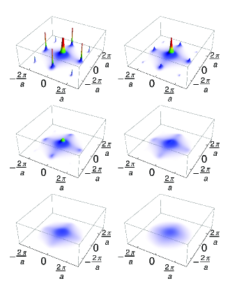
Figure 2: (Color online) Simulation of time-of-flight absorption images [from. Eq. (62)] for various interactions strength $t/U$: transition from superfluid (top-left, $t/U=0.085$) to Mott phase (top-right to the bottom-right $t/U=0.085,\,0.07,\,0.055,\,0.04,\,0.025,\,0.01$, respectively), for $\mu/U=0.5$.

Figure 3: (Color online) Visibility calculated from simulated time-of-flight images as a function of coupling ratio $U/t$ for $\mu/U=0.5$.

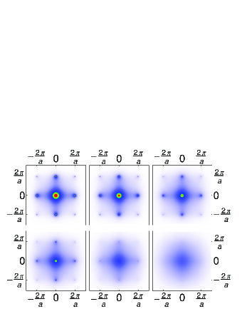
Figure 4: (Color online) Simulated time-of-flight patterns for comparison with experimental time-of-flight absorption images (for values of $V_{0}/E_{R}=7,10,13,14,17,20$, around 150,000 lattice sites and average number of up to 2.5 atoms per lattice site in the center of the trap, chosen as in Ref. [optical_lattices, ], Fig. 2c-h, ).

V Conclusions

In summary, we have studied the correlations of cold atoms loaded in a two dimensional optical lattice. In the superfluid regime the validity of the Bogoliubov approximation is restricted to the very weakly interacting regime ($U/t\ll 1$) and its breakdown as quantum correlations become important. In general Bogoliubov quasi-particle states correspond to solutions of the approximate Hamiltonian with a plane-wave character. As quantum correlations become important, the exact eigenstates of the interacting system do not necessarily have the simple plane wave character, especially in the commensurate filling situation where for a critical value of $U/t$ the system exhibits the superfuid-Mott insulator transition. To address these issues a new theory beyond the simple Bogoliubov approximation was developed that incorporates the phase degrees of freedom via the quantum rotor approach to describe regimes beyond the very weakly interacting one. This scenario provided a picture of quasiparticles and energy excitations in the strong interaction limit, where the transition between the superfluid and the Mott state is be driven by phase fluctuations. Taking advantage of the macroscopically populated condensate state, we have separated the problem into the amplitude of the Bose field and the fluctuating phase that was absent in the original Bogoliubov problem. Subsequently, the functional formulation this formalism was shown to be a powerful tool that incorporates properly the interaction aspects characteristic of the quantum phase dynamics. This formalism provides a useful framework, where the one particle the correlation functions are treated self-consistently and permits us to test and simulate Bose-Hubbard Hamiltonian with a whole range of phenomena. To explore these a diagnostics tools that include spectroscopy of occupation numbers and correlation measurement is called for. Especially, the time of flight imaging is a very powerful technique to probe the quantum gases in optical lattices. From the beginning of the ultra-cold atom field, it permitted to observe the Bose Einstein condensation. In this work we have calculated time-of-flight patterns and the relevant correlation functions on two dimensional optical lattice and compared them with experimental data. Our theoretical pictures match the experimental ones, where one can observe the formation of a central and various neighboring peaks, out of featureless Mott state, which subsequently become sharper in the superfluid phase as a result of a phase coherence. It would be interesting to map out the nature of the Bose transition in optical lattice systems by using further diagnostic tools such as Bragg spectroscopy, which reveals the whole momentum structure of the single particle correlation function. A detailed understanding of this quantity is a challenging task in the further experimental studies of trapped ultra-cold gases.

- (1) M. Greiner, O. Mandel, T. Esslinger , T. W. Hänsch, and I. Bloch, Nature 415, 39 (2002).
- (2) I. Bloch, Nat. Phys. 1, 23 (2005).
- (3) I. Hen and M. Rigol, Phys. Rev. A 82, 043634 (2010).
- (4) In our calculations, we assume that the system is homogeneous, i.e. , with a lattice vector . Since, the system is invariant under translations by integer multiples of lattice vectors (homogeneous), depends only on , but not on the individual sites and .
- (5) F. Gerbier, A. Widera, S. Fölling, O. Mandel, T. Gericke, and I. Bloch, Phys. Rev. A 72, 053606 (2005).
- (6) A. Hoffmann and A. Pelster, Phys. Rev. A 79, 053623 (2009).
- (7) T. P. Polak and T. K. Kopeć, Phys. Rev. B 76, 094503 (2007).
- (8) T. A. Zaleski and T. P. Polak, Phys. Rev. A 83, 023607 (2011).
- (9) N. N. Bogoliubov, J. Phys. Moscow 11, 23 (1947).
- (10) M. P. A. Fisher, P. B. Weichman, G. Grinstein, and D. S. Fisher, Phys. Rev. B 40, 546 (1989).
- (11) S. Sachdev, Quantum Phase Transitions (Cambridge University Press, Cambridge, 1999).
- (12) M. P. A. Fisher, P. B. Weichman, G. Grinstein, and D. S. Fisher, Phys. Rev. B 40, 546 (1989).
- (13) J. K. Freericks and H. Monien, Phys. Rev. B 53, 2691 (1996).
- (14) N. Elstner and H. Monien, Phys. Rev. B 59, 12184 (1999).
- (15) J. K. Freericks, H. R. Krishnamurthy, Y. Kato, N. Kawashima, and N. Trivedi, Phys. Rev. A 79, 053631 (2009).
- (16) T. P. Polak and T. K. Kopeć, J. Phys. B 42, 095302 (2009).
- (17) T. D. Kühner and H. Monien, Phys. Rev. B 58, R14741 (1998).
- (18) S. Rapsch, U. Schollwöck, and W. Zwerger, Europhys. Lett. 46, 559 (1999).
- (19) C. Kollath, U. Schollwöck, J. von Delft, and W. Zwerger, Phys. Rev. A 69, 031601(R) (2004).
- (20) C. Kollath, A. M. Läuchli, and E. Altman, Phys. Rev. Lett. 98, 180601 (2007).
- (21) G. G. Batrouni and R. T. Scalettar, Phys. Rev. B 46, 9051 (1992).
- (22) S. Wessel, F. Alet, M. Troyer, and G. G. Batrouni, Phys. Rev. A 70, 053615 (2004).
- (23) B. Capogrosso-Sansone, N. V. Prokof’ev, and B. V. Svistunov, Phys. Rev. B 75, 134302 (2007).
- (24) B. Capogrosso-Sansone, Ş. G. Söyler, N. Prokof’ev, and B. Svistunov, Phys. Rev. A 77, 015602 (2008).
- (25) T. K. Kopeć, Phys. Rev. B 70, 054518 (2004).
- (26) T. K. Kopeć and J. V. José, Phys. Rev. B 60, 7473 (1999).
- (27) N. Teichmann, D. Hinrichs, M. Holthaus, and A. Eckardt, Phys. Rev. B 79, 224515 (2009).
- (28) T. Vojta, Phys. Rev. B 53, 710 (1996).
- (29) W. Zwerger, J. Opt. B: Quantum Semiclassical Opt. 5, S9 (2003).
- (30) V. A. Kashurnikov, N. V. Prokof’ev, and B. V. Svistunov, Phys. Rev. A 66, 031601R (2002).
- (31) P. Pedri, L. Pitaevskii, S. Stringari, C. Fort, S. Burger, F. S. Cataliotti, P. Maddaloni, F. Minardi, and M. Inguscio, Phys. Rev. Lett. 87, 220401 (2001).
- (32) K. Günter, T. Stöferle, H. Moritz, M. Köhl, and T. Esslinger, Phys. Rev. Lett. 96, 180402 (2006).
- (33) S. Ospelkaus, C. Ospelkaus, O. Wille, M. Succo, P. Ernst, K. Sengstock, and K. Bongs, Phys. Rev. Lett. 96, 180403 (2006).
- (34) F. Gerbier, A. Widera, S. Fölling, O. Mandel, T. Gericke, and I. Bloch, Phys. Rev. Lett. 95, 050404 (2005).
- (35) I. Bloch, J. Dalibard, and W. Zwerger, Rev. Mod. Phys. 80, 885 (2008).
- (36) W. Zwerger, J. Opt. B: Quantum Semiclass. Opt. 5, S9 (2003).