Hysteresis and nonequilibrium work theorem for DNA unzipping

Abstract

We study by using Monte Carlo simulations the hysteresis in unzipping and rezipping of a double stranded DNA (dsDNA) by pulling its strands in opposite directions in the fixed force ensemble. The force is increased, at a constant rate from an initial value $g_{0}$ to some maximum value $g_{m}$ that lies above the phase boundary and then decreased back again to $g_{0}$. We observed hysteresis during a complete cycle of unzipping and rezipping. We obtained probability distributions of work performed over a cycle of unzipping and rezipping for various pulling rates. The mean of the distribution is found to be close (the difference being within $10\%$, except for very fast pulling) to the area of the hysteresis loop. We extract the equilibrium force versus separation isotherm by using the work theorem on repeated non-equilibrium force measurements. Our method is capable of reproducing the equilibrium and the non-equilibrium force-separation isotherms for the spontaneous rezipping of dsDNA.

I Introduction

Unzipping of a double stranded DNA (dsDNA), an essential step in biological processes like DNA replication and RNA transcription, is carried out by enzymes that exert an external force on the strands of the DNA Watson2003 . The phenomenon has been studied both theoretically BhattacharjeeJPA2000 ; LubenskyPRL2000 and experimentally BockelmannBiophysJ2002 ; DanilowiczPRL2004 by applying a pulling force on the strands of the DNA. In theoretical models, the strands of the DNA are modelled either on the lattice, by random or self-avoiding walks, or in the continuum by worm like chains. It was found that when a pulling force is applied on a dsDNA, the two strands unzip if the force exceeds a critical value. Below the critical force the DNA is in the zipped phase while above it the DNA is in the unzipped phase. The force can be applied on the DNA by either keeping the separation between the strands fixed (fixed distance ensemble) or by applying a fixed pulling force (fixed force ensemble) on the strands. For the later case, the separation between the strands fluctuates while it is the force needed to keep the separation fluctuates in the fixed distance ensemble. The unzipping of dsDNA by a pulling force is a first-order phase transition BhattacharjeeJPA2000 ; LubenskyPRL2000 .

In a continuous phase transition large fluctuations in the order parameter are present near the transition region that act as a precursor that something unusual is about to occur. In the case of DNA, if the melting is continuous, there will be large fluctuations in the size and shape of the denatured bubbles along the chain. These fluctuations are absent in a first-order phase transition and the order parameter changes abruptly as the phase boundary is crossed. However, there is usually a hysteresis associated with the first order transition which causes the change to occur at a point that is slightly displaced from the phase boundary. This is because at a first order phase boundary the two phases can coexist and be separated by interfaces. The energy of the interface acts as a barrier between two phases. Hysteresis is often linked to the dynamics of interfaces. Some aspects of interfaces in DNA have been discussed in Ref. SadhukhanEPL2011 . Near the phase boundary, there is a region of metastability where the system can stay in its previous phase even after crossing the phase boundary. From the dynamics point of view, the relaxation time or the time scale to cross the barrier becomes large near the transition and therefore, there is a conflict between relaxation and the time scale of change of parameters. This produces hysteresis. A classic example of first-order transition in which hysteresis has been studied in detail is the Ising model below the critical temperature in an external magnetic field ChakrabartiRMP1999 . In recent years, hysteresis has been studied in unbinding and rebinding of biomolecules under a pulling force by using single molecule manipulation techniques HatchPRE2007 ; FriddleJPCC2008 ; TshiprutJCP2009 because it can provide useful information on kinetics of conformational transformations, potential energy landscape, and controlling the folding pathway of a single molecule LiPNAS2007 .

The equilibrium statistical mechanics is a celebrated framework that gives the microscopic description of the thermodynamics of the system. However, one major challenge, often faced in designing experiments, is the requirement of thermodynamic equilibrium; the system should remain in equilibrium, or at least at quasi-equilibrium, throughout the course of the experiment, and needs to be equilibrated whenever system parameters are changed. However, in the last decade many remarkable identities, known as nonequilibrium work or fluctuation theorems (see Ref. EvansAP2002 for a review), are developed that bridges the gap between the nonequilibrium and equilibrium statistical mechanics. One of them is the Jarzynski equality (JE) JarzynskiPRL1997 , which connects the thermodynamic free-energy differences between the two equilibrium states (say $A$ and $B$), $\Delta F=F_{B}-F_{A}$, and the irreversible work done, $W$, in taking the system from one equilibrium state $A$ to a non-equilibrium state having the same external conditions as that of the other equilibrium state $B$. The relation between $\Delta F$ and $W$ is

$$e^{-\Delta F/k_{B}T}=\langle e^{-{W}/{k_{B}T}}\rangle,$$ (1)

where $k_{B}$ is the Boltzmann constant and $T$ is the absolute temperature. The bracket $\langle\cdots\rangle$ denotes average over all possible paths between $A$ and $B$. Recently, Sadhukhan and Bhattacharjee SadhukhanJPA2010 have given a dynamics-independent nonequilibrium path integral formulation of the JE that can easily be generalized to cases involving parameters like temperature and interactions. The applicability of JE has been questioned for boundary-switching processes. It was shown that for spontaneous irreversible processes (e.g., the adiabatic expansion of the gas into vacuum) the JE is not satisfied SungPRE2008 . However, our simulations show that one can get the equilibrium information by using JE and the multiple histogram technique FerrenbergPRL1989 even for the spontaneous rezipping of dsDNA.

In this paper we study the hysteresis in unzipping and rezipping of a homopolymer dsDNA when its strands are pulled in opposite directions by a force. The force $g$ is increased, at a constant rate $\dot{g}\equiv\Delta g/\Delta t$, from some initial value $g_{0}$ to some maximum value $g_{m}$ that lies above the phase boundary. The force $g$ is then decreased back to $g_{0}$ at the same rate. We observed hysteresis during a complete cycle of unzipping and rezipping. By using the work theorem on repeated non-equilibrium force measurements on the forward and the backward paths, we extract the equilibrium force-distance isotherm. We also show that our procedure can be used to obtain the complete equilibrium and nonequilibrium force-separation isotherms for the spontaneous rezipping of dsDNA. In this process, the dsDNA is initially at equilibrium with a maximum pulling force $g=g_{m}$ and the force is suddenly decreased to a minimum force $g=g_{0}$.

The paper is organized as follows: In Sec. II, we define our model and the details of the Monte Carlo simulations. We compare the equilibrium results obtained by the simulation with the exact results known for the model. The results are discussed in Sec. III and summarized in Sec. IV.

II Model

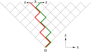
The two strands of a homo-polymer DNA are represented by two directed self-avoiding walks on a $d=1+1$ dimensional square lattice. The walks starting from the origin are restricted to go towards the positive direction of the diagonal axis ($z$-direction) without crossing each other. The directional nature of the walks takes care of self-avoidance and the correct base pairing of DNA, that is, the monomers which are complementary to each other are allowed to occupy the same lattice site. For each such overlap there is a gain of energy $-\epsilon$ ($\epsilon>0$). One end of the DNA is anchored at the origin and a force $g$ acts along the transverse direction ($x$-direction) at the free end. The schematic diagram of our model is shown in Fig. 1.

Figure 1: (Color online) Schematic diagram of DNA unzipping. The strands of the DNA are shown by thick solid lines with a pulling force $g$ act along $x$ direction at end monomers.

Let $D_{n}(x)$ be the partition function in the fixed distance ensemble of a dsDNA of length $n$ with separation $x$ between the $n$th monomers of two strands. $D_{n}(x)$ satisfies the following recursion relation:

$$D_{n+1}(x) = \left[D_{n}(x+1)+2D_{n}(x)+D_{n}(x-1)\right]$$ (3)

$$\qquad\qquad\qquad\times\left[1+\left(e^{\beta\epsilon}-1\right)\delta_{x,0}\right],$$

with an initial condition $D_{0}(x)=e^{\beta\epsilon}\delta_{x,0}$.

The above recursion relation can be solved exactly via the generating function technique MarenduzzoPRE2001 ; MarenduzzoPRL2002 ; KapriPRL2004 . The aim is to calculate the singularities of the generating function. The singularity closest to the origin gives the phase of the DNA and the phase transition takes place when two singularities cross each other. The generating function for $D_{n}(x)$ can be taken of the form (ansatz)

$$\hat{D}(z,x)=\sum_{n}z^{n}D_{n}(x)=\lambda^{x}(z)A(z).$$ (4)

When used in the above recursion relation, we obtain $\lambda(z)=(1-2z-\sqrt{1-4z})/(2z)$ and $A(z)=1/\left[1-z\left(2+\lambda(z)\right)e^{\beta\epsilon}\right]$. The singularities of $\lambda(z)$ and $A(z)$ are $1/2$ and $z_{2}=\sqrt{1-e^{-\beta\epsilon}}-1+e^{-\beta\epsilon}$ respectively. The zero force melting, which comes from $z_{1}=z_{2}$, takes place at a temperature $T_{m}=\epsilon/\ln(4/3)$. In the large length limit, $D_{n}(x)$ can be approximated as $D_{N}(x)\approx\lambda^{x}(z_{2})/z_{2}^{N+1}$, with the free energy $\beta F=N\ln z_{2}-x\ln\lambda(z_{2})$. The force required to maintain the separation $x$ is then given by

$$g(T)=\frac{\partial F}{2\partial x}=-\frac{k_{B}T}{2}\ln\lambda(z_{2}),$$ (5)

where $2$ in the denominator is the unit length of the diagonal of the square lattice. In the fixed force ensemble, the generating function can be written as

$$\mathcal{G}(z,\beta,g) = \sum_{x}e^{2\beta gx}\sum_{n}z^{n}D_{n}(x)=\sum_{x}e^{2\beta gx}\lambda^{x}(z)A(z)$$ (6)

$$= \frac{A(z)}{1-\lambda(z)e^{2\beta g}},$$ (7)

which has an additional force dependent singularity $z_{3}=1/[2+2\cosh(2\beta g)]$. The phase boundary comes from $z_{2}=z_{3}$, and is given by

$$g(T)=\frac{k_{B}T}{2}\cosh^{-1}\left[\frac{1}{2}\frac{1}{\sqrt{1-e^{-\beta\epsilon}}-1+e^{-\beta\epsilon}}-1\right],$$ (8)

which is same as the phase boundary obtained in the fixed distance ensemble. The phase diagram for $k_{B}=1$ is shown in Fig. 2(a). The phase diagrams of DNA unzipping has been obtained previously in Refs. MarenduzzoPRE2001 ; MarenduzzoPRL2002 ; KapriPRL2004 .

Figure 2: (Color online) (a) Critical unzipping force as a function of temperature [Eq. (5)]. (b) Force $g$ vs equilibrium average separation $\langle x\rangle_{eq}$ between the end monomers of the dsDNA at $T=1.0$. The line is from the exact transfer matrix approach and points are from the Monte Carlo simulations. (c) Typical equilibrium configurations of the dsDNA of length $N=128$ for force values $g=0.65$ (lies just below the phase boundary) and $g=0.9$ (far above the phase boundary) at $T=1.0$ obtained by using Monte Carlo simulations. The lines are the bonds between monomers of the strands.

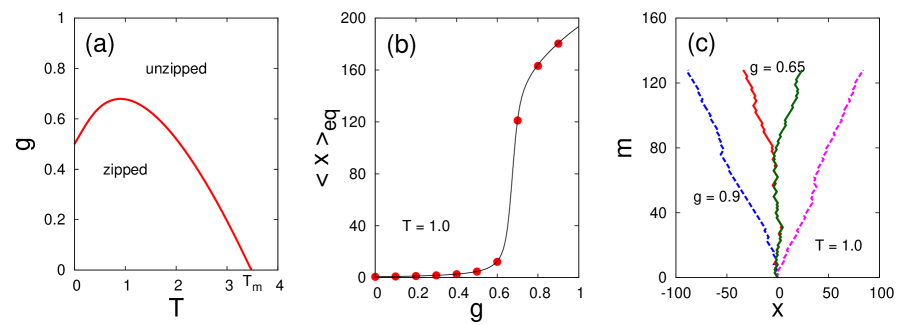
For many other equilibrium properties, based on thermal averaging, the exact transfer matrix technique can be used to obtain numerically the partition function $D_{N}(x)$ for the DNA of length $N$. This technique gives exact numerical results for finite $N$, which is rather difficult in the generating function method. To obtain $D_{N}(x)$ at any given temperature we start with an initial condition $D_{0}(0)=1$ and iterate the above recursion relation [i.e. Eq.(3)] $N$ times. The equilibrium average separation between the end monomers, $\langle x\rangle_{\rm eq}$, can then be obtained by

$$\langle x\rangle_{\rm eq}=\frac{\sum_{x}x\ D_{N}(x)e^{\beta gx}}{\sum_{x}D_{N}(x)e^{\beta gx}},$$ (9)

which is shown in Fig. 2(b) for a DNA of length $N=128$ at $T=1.0$.

In this paper, to go beyond equilibrium, we perform Monte Carlo simulations of the model by using the Metropolis algorithm, which allows us to study both equilibrium and off-equilibrium behaviors. The strands of the DNA undergo Rouse dynamics that consists of local corner-flip or end-flip moves Doi1986 that do not violate mutual avoidance (the self-avoidance is taken care by the directional nature of the walks). The elementary move consists of selecting a random monomer from a strand, which itself is chosen at random, and flipping it. If the move results in overlapping of two complementary monomers, thus forming a base-pair between the strands, it is always accepted as a move. The opposite move, that is, the unbinding of monomers, is chosen with the Boltzmann probability $\eta=\exp(-\epsilon/k_{B}T)$. If the chosen monomer is unbind, which remains unbind after the move is performed is always accepted. The time is measured in units of Monte Carlo steps (MCSs). One MCS consists of $2N$ flip attempts, that is, on an average, every monomer is given a chance to flip. Throughout the simulation, the detailed balance is always satisfied. From any starting configuration, it is possible to reach any other configuration by using the above moves. Throughout the paper, without loss of generality, we have chosen $\epsilon=1$ and $k_{B}=1$.

To check if the results obtained by using the above mentioned moves are consistent with the analytical results obtained previously, we calculate the force $g$ vs equilibrium average separation $\langle x\rangle_{\rm eq}$ between the end monomers of the DNA of length $N=128$ at $T=1$. This is shown in Fig. 2(b) by filled circles. Every data point is obtained by first equilibrating the system for $2\times 10^{5}$ MCSs and then averaged over $10^{4}$ different realizations. In the same plot we have also shown, by solid line, the force-distance isotherm obtained by using the exact transfer matrix calculations for the model. The results of Monte Carlo simulations match excellently with the exact result. The equilibrium configurations of the dsDNA of length $N=128$ at temperature $T=1$ for two different forces $g=0.65$, which lies just below the phase boundary, and $g=0.9$, which is far away from the phase boundary (and also the maximum force used in this paper at $T=1$) are also shown in Fig. 2(c). These configurations show that the DNA is in the zipped phase (with a small Y-fork at the end) for the force below the critical force and in the unzipped phase for the force above the critical force.

To study the hysteresis in DNA, we start the simulation with a valid configuration of a dsDNA of length $N=128$ at $T=1$ and $N=256$ at $T=3.6$. The later temperature is above the melting temperature $T_{m}\approx 3.476$ of the dsDNA for the model used in this paper. The system is first equilibrated with zero pulling force $g_{0}=0$. The force $g$ is incrementally increased from $g_{0}$ to $g_{m}=0.9$ at $T=1$ ($g_{m}=1.0$ is used at $T=3.6$) at a step of $\Delta g^{F}=0.01$ by using the following protocol

$$g_{i}^{F}=g_{0}+i\Delta g^{F},$$ (10)

where $i=0,1,2,\ldots,n$ with $n=(g_{m}-g_{0})/\Delta g^{F}$ is the number of steps between the initial and the final force values. The superscript $F$ denotes the forward path. For the backward path (denoted by superscript $B$) the force is incrementally decreased from $g_{m}$ to $g_{0}$ by $\Delta g^{B}=-\Delta g^{F}$. The number of steps $n$ and the time interval $\Delta t$ are kept same as that of the forward path.

Each step of the process can be thought of two substeps. In the first substep, the force is increased by $\Delta g^{F}$. Therefore, an amount of work $\Delta W^{F}=-\Delta g^{F}x_{i}^{F}$ has to be performed on the system, where $x_{i}^{F}$ is the separation between the end monomers of the DNA at the beginning of the $i$th step. In the second step, the system is relaxed for the time interval $\Delta t$ in the presence of the pulling force $g_{i+1}$. The total work performed on the system during the complete forward process is

$$W^{F}=-\Delta g^{F}\sum_{i=0}^{n-1}x_{i}^{F}.$$ (11)

Similarly, for the backward path the work performed by the system is

$$W^{B}=-\Delta g^{B}\sum_{i=0}^{n-1}x_{i}^{B}.$$ (12)

The above procedure is repeated many times to obtain various trajectories. For each realization, the system is initially equilibrated at $g_{0}$ but no attempt has been made to equilibrate the system at the maximum force $g_{m}$ used in this paper. The total work done over a complete unzipping and rezipping cycle is given by the sum of the work performed along the forward and the backward paths

$$W=W^{F}+W^{B}.$$ (13)

The work performed $W$ is different for different realizations. The following sign convention is adopted in this paper: The positive (negative) sign of work denotes the work done on the system (by the system).

III Results and Discussions

Before discussing our results let us fix some notations to avoid confusion. We are working in the fixed force ensemble and define the pulling rate by $\dot{g}\equiv\Delta g/\Delta t$. We fix the force interval to $\Delta g=0.01$ (in magnitude) for both the forward and the backward paths and change the time interval $\Delta t$ to change the pulling rate. Therefore, instead of giving the actual numerical value we just give the time interval $\Delta t$ for the pulling rate. For example, the pulling rate for $\Delta t=100$ means $\dot{g}\equiv 0.01/100=10^{-4}$.

III.1 Hysteresis curves

Figure 3: (Color online) (a) The separation $x$ between the end monomers of the DNA as a function of force $g$ for the forward (unzipping) and the backward (rezipping) paths for two different realizations of a dsDNA of length $N=128$ at $T=1$ for the pulling rate $\Delta t=1000$. The filled and the open symbols represent the forward and the backward paths, respectively. The work done over a complete cycle is negative (positive) for the realization shown by circles (diamond). (b) Hysteresis curves for different pulling rates. The equilibrium curve, shown by the filled circles, does not show any hysteresis. The paths are averaged over $10^{5}$ different realizations.

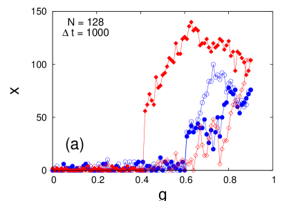
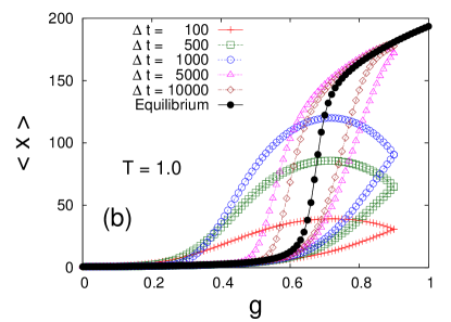
In Fig. 3(a), we have shown, for two different realizations, the force $g$ versus separation $x$ between the end monomers of dsDNA for the pulling rate for $\Delta t=1000$. The forward and backward paths are shown respectively by open and filled symbols. These realizations reveal that the system does not get enough time to relax to the equilibrium and shows hysteresis. The average separation $\langle x\rangle$ at force $g$ is obtained by

$$\langle x\rangle=\frac{1}{M}\sum_{i=1}^{M}x_{i},$$ (14)

for both the forward and backward paths. The resulting hysteresis for various pulling rates averaged over $M=10^{5}$ realizations are shown in Fig. 3(b). When $\Delta t$ is smaller (i.e., the pulling rate is higher), the system does not get enough time to respond to the change in the pulling force and the average separation between the strands is small even if the pulling force is greater than the critical force needed to unzip the DNA. On decreasing the force from the maximum, the separation between the strands initially increases because the force is still greater than the critical unzipping force and the system gets some more time to relax. Therefore, on the backward path there exist a force at which the average separation is equal to the equilibrium separation. This is the point at which the equilibrium curve cuts the backward path of the hysteresis loop in Fig. 3(b). On decreasing the force further, the average separation decreases slowly and the system is again driven away from the equilibrium. If we join the forward and the backward paths we get a small hysteresis loop. The area of the loop gives the amount of heat that is deposited to the system. Since for the fast pulling rate (i.e., small $\Delta t$) only a small segment of the dsDNA can be opened by the force, the area of the loop is small. As $\Delta t$ is increased, the system gets more and more time to respond to the change in the pulling force and the average separation between the strands at $g_{m}$ increases. This increase in separation continues initially on the backward path also and therefore the area of the hysteresis loop increases as is visually seen from Fig. 3(b). But the area of the loop cannot increase forever with the increase of $\Delta t$. For sufficient large $\Delta t$, the average separation between the strands at $g_{m}$ becomes closer to the equilibrium separation as can be seen for $\Delta t=10000$ curve. We will see later that for such cases, the nonequilibrium measurements along the backward paths can also be used to calculate the equilibrium curve. If $\Delta t$ is very large, that is, the pulling is very slow, the system gets sufficient time to get equilibrated before the force is increased to a new value. Therefore, the system remains in equilibrium for all force values and does not show any hysteresis (zero loop area). This situation is shown in Fig. 3(b) by filled circles. The area of the hysteresis loop calculated by integrating numerically using trapezoidal rule for various $\Delta t$ values are tabulated in Table I, which confirms the above statement.

$\Delta t$	$\langle W\rangle$	$\sigma$	Area of
			hysteresis loop
100	$10.3\pm 0.3$	$8.0\pm 0.3$	12.636
500	$25.6\pm 0.2$	$12.8\pm 0.2$	28.057
1000	$37.5\pm 0.2$	$14.3\pm 0.2$	38.066
5000	$26.17\pm 0.03$	$6.75\pm 0.03$	27.687
10000	$16.33\pm 0.02$	$5.47\pm 0.02$	18.029
12000	$14.42\pm 0.05$	$5.12\pm 0.05$	16.138

Table 1: The average $\langle W\rangle$ and the standard deviation $\sigma$ of the probability distribution of work performed over an unzipping and rezipping cycle, and the area of the hysteresis loop for various $\Delta t$ values.

III.2 Probability distribution of work performed over a cycle

As stated in Sec. II, the work performed during a complete unzipping and rezipping cycle are different for different realizations. There are a few realizations for which the work obtained during the rezipping process is more than the work performed during the unzipping process. One such realization is shown in Fig. 3(a) by circles. The second law of thermodynamics cannot be violated. But if one looks at an individual or a group of such trajectories, there is an illusion of a violation. However, for the majority of trajectories, which look more or less like the realization shown in Fig. 3(b) by diamonds, the work performed during the unzipping process is more than the work obtained during the rezipping process. The probability distribution of work guarantees that the second law of thermodynamics is satisfied on an average.

Figure 4: (Color online) Probability distribution P(W), of the work performed during a complete unzipping and rezipping cycle for various $\Delta t$ values. The solid lines are the Gaussian fit to the distributions while the dashed line for $\Delta t=100$ is guide to eyes.

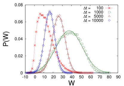
In Fig. 4, we have plotted the probability distribution of work, $P(W)$, performed over a complete unzipping and rezipping cycle for various $\Delta t$ values. The solid lines are the Gaussian fit to the data

$$P(W)=A\exp\left[-\frac{(W-\langle W\rangle)^{2}}{2\sigma^{2}}\right],$$ (15)

where, $\langle W\rangle$ and $\sigma$, respectively, represent the average work performed during a cycle and the standard deviation of the distribution and $A$ is the normalization constant. The values obtained for various $\Delta t$ are tabulated in Table I.

One can observe from the figure that for $\Delta t=100$ (i.e., for faster pulling rates), the probability distribution deviates from the Gaussian distribution. The asymmetry of the distribution is quite visible, so we have not shown the Gaussian fit for this data but joined data points by a dashed line to guide the eyes. The distribution is peaked towards lower $W$ values and therefore the probability of obtaining negative work over a cycle is also higher. The average work is however positive. As the pulling rate decreases, the distribution becomes more and more symmetric and tend towards the Gaussian distribution. The peak of the distribution first shifts towards higher $W$ values and it becomes broader as can be seen in the figure for $\Delta t=1000$. On decreasing the pulling rate further, the mean and the width of the distribution again starts decreasing. If the pulling rate is extremely slow, the system remains in equilibrium at all times during the forward and the backward path, and therefore the work done on the system during the forward path is exactly equal to the work done by the system during the backward path. The total work performed over a cycle is zero and the distribution $P(W)$ is sharply peaked at $W=0$. Therefore, at equilibrium, the average work done on the system is exactly equal to the area of the hysteresis loop. In the nonequilibrium regime, except for very fast pulling rate (i.e., $\Delta t=100$), the difference of the average work done on the system and the area of the hysteresis loop is within $10\%$ (see Table I) of the area of the loop. The difference comes because only $10^{5}$ trajectories are simulated. This many trajectories are good enough to calculate the average extensions and hence the area of the hysteresis curves. However, these are not good enough to calculate the probability distributions of the work, which are obtained by binning the data. If more realizations are used in obtaining the probability distributions the difference between the two quantities will become smaller.

For a cyclic process, the initial and the final equilibrium states are the same. Substituting $\Delta F=0$ in Eq. (1) one gets

$$Z\equiv\langle e^{-\beta W}\rangle\equiv\frac{1}{M}\sum_{i=1}^{M}e^{-\beta W_{i}}=1.$$ (16)

This equality strictly holds for infinite trajectories $M\to\infty$. The convergence is often slow because it picks up exponential weights and the trajectories that contribute to the sum (i.e. having extreme weights) are rare. We calculate $Z$ for $\Delta t=10000$ case. On averaging over $M=10^{2},10^{3},10^{4}$, and $10^{5}$ trajectories, we obtain $Z=0.0027,0.0102,0.0827$, and $0.2784$, respectively. This shows that $Z$ increases with number of trajectories used in averaging. This direct sum over paths may not be a useful numerical way to estimate the free-energy or establish Eq. (16). However, a weighted average as discussed below is more efficient for averages. The probability distributions $P(W)$ obtained above can be used to calculate $Z$:

$$Z=\int_{-\infty}^{\infty}dWe^{-\beta W}P(W)=\exp\left(-\beta\langle W\rangle+\frac{\beta^{2}\sigma^{2}}{2}\right).$$ (17)

Substituting the value of $\langle W\rangle$ and $\sigma$ for $\Delta t=10000$ from Table I, we get $Z=0.2542$, which is somewhat smaller than the value obtained from Eq. (16) for $10^{5}$ trajectories. Equation (17) is not applicable for fast pulling (i.e., smaller $\Delta t$ values) because of deviations from Gaussian. For those cases, higher cumulants are important. In the limit of infinite trajectories, $P(W)$ will become the true probability distribution of work and the value of $Z$ obtained by either methods will approach $1$.

III.3 Equilibrium curves from non-equilibrium measurements

In this section, we discuss the procedure that can be used to obtain the equilibrium force-distance isotherms by using non-equilibrium measurements on the forward and the backward paths. Our technique is similar to that of Hummer and Szabo HummerPNAS2001 , but in the conjugate ensemble). The above method (Ref. HummerPNAS2001 ) has been used successfully to obtain the zero force free energy on single molecule pulling experiments in constant velocity ensemble GuptaNPhys2011 .

Figure 5: (Color online) Hysteresis obtained in unzipping and rezipping of a dsDNA for various pulling rates at two different temperatures, (a) to (c) at $T=1.0<T_{m}$ and (d) to (f) at $T=3.6>T_{m}$. The forward (shown by dashed line) and the backward (shown by dotted line) paths are averaged over $10^{5}$ realizations for (a) and (b) while for cases (c) to (f) paths are averaged over $10^{4}$ realizations. The unfilled and filled circles represent the equilibrium curves obtained by using work theorem on nonequilibrium forward and backward paths, respectively. The solid lines represent the equilibrium curves obtained by using the exact transfer matrix technique.

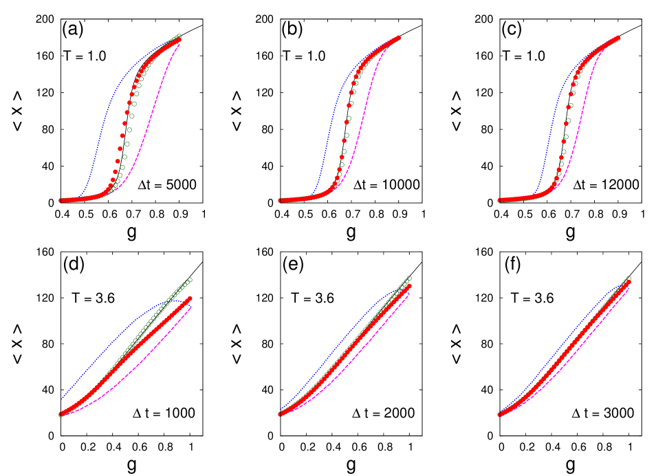
In Figs. 5(a), 5(b) and 5(c), we have plotted the hysteresis loops for $\Delta t=5000$, $10000$, and $12000$, and the equilibrium curve obtained by using the exact transfer matrix for $N=128$ and $T=1$, which is below the melting temperature $T_{m}=3.476$. In the same plot we have also shown the equilibrium data calculated from the nonequilibrium force measurements by using the procedure described below.

We divide the forward path into intervals of sizes $\Delta g$. Let $i$ and $k$ represent respectively the indices for the sample and the force. The irreversible work done over the $i$th non-equilibrium path, taking $W_{i0}=0$ at $g_{0}$, is given by

$$W_{ik}=-\Delta g\sum_{j=0}^{k}x_{ij}.$$ (18)

By using $\exp(-\beta W_{ik})$ as the weight for path $i$, the equilibrium separation between the end monomers of the dsDNA, $x_{k}^{\rm eq}$, at force $g_{k}$ can be obtained by

$$x_{k}^{\rm eq}=\frac{\sum_{i=1}^{M}x_{ik}\exp\left(-\beta W_{ik}\right)}{\sum_{i=1}^{M}\exp\left(-\beta W_{ik}\right)}.$$ (19)

The above procedure has been used by Sadhukhan and Bhattacharjee SadhukhanJPA2010 to obtain the equilibrium curve.

Figure 6: (Color online) The equilibrium curves, shown by unfilled (filled) circles for the forward (backward) paths, obtained by using work theorem on nonequilibrium paths when the backward paths are also initially equilibrated at $g_{m}$. The dashed and dotted lines are, respectively, the forward and backward nonequilibrium paths averaged over $10^{4}$ realizations at $T=3.6$ for various pulling rates. The solid line represent the equilibrium curve obtained by using the exact transfer matrix technique.

In our simulation, we have $10^{5}$ $x_{k}$ values, at each force $g_{k}$. These values can be used in Eq. (19) to obtain $x_{k}^{\rm eq}$ at $g_{k}$. However, one can do better than this. For a given temperature $T$ and force $g$, the system at equilibrium samples a narrow phase space given by the Boltzmann distribution. The distributions at nearby force values overlap with each other. The overlapping distributions can be properly weighted to obtain the approximate density of states (DOS) of the system. This goes by the name of multiple histogram technique FerrenbergPRL1989 and has been exploited in simulations. Once the DOS is known, the observables can be calculated at any other force. To achieve this we build up the histogram $H_{k}(x)$ at force $g_{k}$. For the $i$th realization, if the separation is $x$, we increment the corresponding histogram value by $\exp(-\beta W_{ik})$,

$$H_{k}(x)=\sum_{i=1}^{M}e^{-\beta W_{ik}}\ \delta_{x,x_{i}},$$ (20)

where, $\delta_{x,x_{i}}=1$ if $x=x_{i}$, and zero otherwise. The partition function $Z_{k}$ at force $g_{k}$, obtained by using the multiple histogram technique FerrenbergPRL1989 , reads as

$$Z_{k}=\sum_{x}\rho(x)\exp(\beta g_{k}x),$$ (21)

where

$$\rho(x)=\frac{\sum_{j}\frac{H_{j}(x)}{Z_{j}}}{\sum_{j}\frac{\exp(\beta g_{j}x)}{Z_{j}}},$$ (22)

is the DOS. Equation (21) needs to be evaluated self-consistently. We take initial $Z_{k}$’s as

$$Z_{k}=\frac{1}{M}\sum_{i=1}^{M}\exp\left(-\beta W_{ik}\right),$$ (23)

and iterate Eq. (21) till it converges to a true DOS. The initial values are motivated by the JE [see Eq. (1)]. By using $\rho(x)$, we can then evaluate the equilibrium separation $x_{k}^{\rm eq}$ at force $g_{k}$ by

$$x_{k}^{\rm eq}=\frac{1}{Z_{k}}\sum_{x}x\rho(x)\exp(\beta g_{k}x).$$ (24)

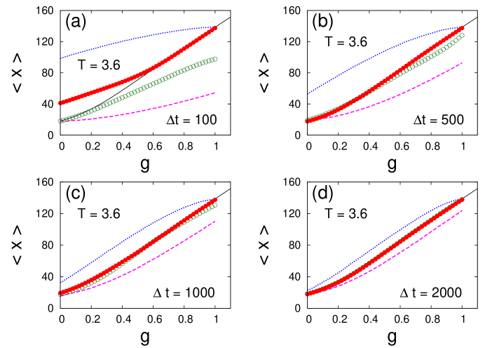
The equilibrium force-separation curve obtained by using the data of $10^{5}$ nonequilibrium forward paths for $\Delta t=5000$ and $10000$, and $10^{4}$ paths for $\Delta t=12000$, in above procedure is shown by open symbols in Figs. 5(a)- 5(c). The data for $\Delta t=10000$ and $12000$ match reasonably well with the equilibrium curve obtained by the exact transfer matrix method. The same procedure can also be adopted for the backward path. The equilibrium force-extension curve obtained by using the nonequilibrium data for the backward path is shown by filled circles which match excellently with the exact curve for $\Delta t=10000$ and $12000$. For the fast pulling case, that is, $\Delta t=5000$, the results from the forward paths match all other points except at the transition region due to poor statistics in that region. The multihistogram approach, by analyzing the errors in the estimates of the partition function, tries to correct for the unexplored part of the phase space. Even for this to work, one needs good sampling or better statistics. The other approach is to generate rare conformations that have dominant contributions in the weighted sum by using special algorithms SunJCP2003 ; YtrebergJCP2004 ; OberhoferPRE2007 . It would be interesting to do a comparative study of the two approaches. Special algorithms are important in generating trajectories for very fast pulling rates (e.g., $\Delta t=100$, $500$, etc.), where not enough rare configurations can be generated by simply including more trajectories due to low probabilities of such configurations. We have also shown, in Figs. 5(d)- 5(f), the hysteresis and equilibrium curves obtained by using the above procedure for $N=256$ at temperature $T=3.6$ which is above the melting temperature of the DNA. These are obtained for the pulling rates with $\Delta t=1000$, $2000$ and $3000$ respectively by averaging over $10^{4}$ nonequilibrium paths. The equilibrium curve obtained by using the data of the forward paths match excellently with the exact curve while the curve that uses the data of the backward paths deviates from the exact curve at higher forces. As stated previously, we have not made any attempt to equilibrate the system at the maximum force $g_{m}$. Still, we could get an excellent match with the equilibrium curve by using the data for the backward paths for $T=1$ but not with the data for $T=3.6$. This can be understood by observing the hysteresis curves near $g_{m}$ for both cases. For $T=1$, with $\Delta t=10000$ and $12000$, the average separation between the end monomers of the DNA at $g_{m}$ is quite closer to the equilibrium curve. Therefore, the system is practically in equilibrium at the beginning of the backward paths and one can use the work theorem [Eq. (1)] to obtain equilibrium properties. However, for $T=3.6$, the system has not reached the equilibrium at $g_{m}$ and so the requirement of work theorem, that is, the system should initially be in equilibrium, is not satisfied for the backward paths and it cannot be applied for this case. If we allow initial equilibration at the maximum force $g_{m}$ then the work theorem can be applied for the backward paths also and the weighted data on the backward paths should give us the equilibrium curve. This we have explored at $T=3.6$ for various $\Delta t$ values in Fig. 6. One can see from the figure that for $\Delta t=500$, $1000$, and $2000$, the curves obtained by using our procedure on $10^{4}$ nonequilibrium trajectories match reasonably well with the exact curve. For $\Delta t=100$, which is the fastest pulling rate reported in this paper, the curves deviate from the exact curve at other ends but this is due to the poor statistics in that region. In Fig. 7, we have shown how these curves behave when the weighted average is taken over a different number ($10^{3}$, $10^{4}$ and $10^{5}$) of trajectories. On including more trajectories, we can see that the curves move towards the exact equilibrium curve. To get better statistics in the fast pulling regime, one can use algorithms SunJCP2003 ; YtrebergJCP2004 ; OberhoferPRE2007 mentioned previously to generate rare trajectories. These can be included in the above procedure to get a better match but we have not attempted it in this paper. It is clear from the above discussion that the above procedure can be used successfully to obtained the equilibrium force-separation isotherms from the nonequilibrium measurements when a pulling force is applied on the strands of the dsDNA that varies with a constant rate.

Figure 7: (Color online) Equilibrium $g$ versus $\langle x\rangle$ isotherms obtained by using work theorem on $10^{3}$, $10^{4}$, and $10^{5}$ nonequilibrium trajactories for the pulling rate $\Delta t=100$ at $T=3.6$. The unfilled (filled) circles represent the forward (backward) path. The solid lines represent the exact equilibrium curve.

Figure 8: (Color online) Equilibrium and nonequilibrium $g$ versus $\langle x\rangle$ isotherms obtained by using a work theorem on $10^{4}$ trajactories when the pulling force on the DNA decreases spontaneously from $g_{m}=0.725$ to various $g_{0}$ values as indicated. The unfilled (filled) symbols represent the equilibrium (nonequilibrium) curves. The solid line represent the exact equilibrium curve and dotted lines are a guide to eyes.

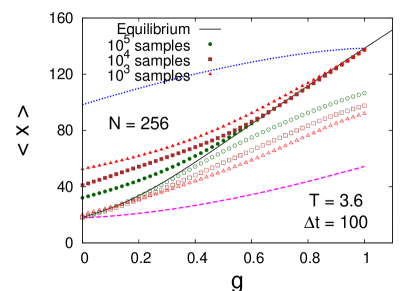
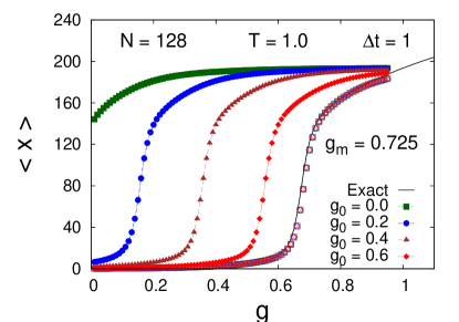
To check the robustness of the above method, we study the spontaneous rezipping of dsDNA. The DNA is initially equilibrated with a pulling force $g_{m}=0.725$ at a temperature $T=1$. The force $g_{m}$ lies above the phase boundary (but close to it) and the dsDNA is in the unzipping phase. The force is suddenly decreased to a lower value $g_{0}$ that lies below the phase boundary in which the DNA is in the zipped phase (i.e., a different boundary condition than $g_{m}$). From the initial to the final force, the system is equilibrated for $1$ MCS (i.e., $\Delta t=1$). It is interesting to know if the method discussed above is capable of predicting the equilibrium and the nonequilibrium force-separation curves at various other force values. In Fig. 8 we have shown the curves obtained by using the above method with $10^{4}$ trajectories when the force is spontaneously decreased from $g_{m}=0.725$ to $g_{0}=0.6$, $0.4$, $0.2$, and $0.0$. The equilibrium (nonequilibrium) curves are shown by the unfilled (filled) symbols. An excellent match with the exact force-separation isotherm shows that the above method can be used to predict the equilibrium force-separation isotherms from the spontaneous rezipping of dsDNA. The application range of the above method is limited by how good statistics of the end separation one can get. The maximum force $g_{m}=0.725$ is chosen near the phase boundary because, even though the DNA is in the unzipped phase, many configurations exist, which is needed to sample the whole phase space. If we take $g_{m}$ far away from the phase boundary, the unzipped phase will only have fully stretched configurations and isotherms extracted by the above method will deviate from the exact result at smaller force values due to poor statistics in that region. The fact that the spontaneous unzipping is capable of reproducing the exact equilibrium force-separation isotherms makes the above method an excellent candidate for analyzing the pulling experiments. It, however, needs to be explored further. The detailed analysis will be published elsewhere.

IV Concluding Remarks

To summarize, we have studied the hysteresis in unzipping and rezipping of a dsDNA in the fixed force ensemble. We found that the area of the hysteresis loop depends on the pulling rate. For fast pulling the area of the loop is smaller. On decreasing the pulling rate, the area of the loop first increases, and then starts decreasing due to the system’s proximity to the equilibrium for the sufficiently slow pulling rates. On decreasing the pulling rate further, the system remains in equilibrium at all intermediate force values and the area of the loop becomes zero. We obtained the probability distributions of work performed over a complete unzipping and rezipping cycle for various pulling rate. The average of this distribution is found to be very close (the difference being within $10\%$, except for very fast pulling i.e. $\Delta t=100$) to the area of the hysteresis loop. We also discussed a procedure to obtain equilibrium force-distance isotherms by using repeated non-equilibrium measurements on the forward paths. We found that if the pulling rate is such that the average separation between the end monomers at the maximum force used is close to the equilibrium curve, the backward path gives better results than the forward paths. Furthermore, using our technique, one can obtain the complete equilibrium and the non-equilibrium force-separation isotherms for the spontaneous rezipping of dsDNA. We believe that our multiple histogram based algorithm using work theorem can be implemented in molecular manipulation machines to provide both the equilibrium and the nonequilibrium information for pulling experiments.

References

- (1) J. D. Watson et al., Molecular Biology of the Gene, th ed. (Pearson/Benjamin Cummings, Singapore, 2003).
- (2) S. M. Bhattacharjee, J. Phys. A 33, L423 (2000).
- (3) D. K. Lubensky and D. R. Nelson, Phys. Rev. Lett. 85, 1572 (2000).
- (4) U. Bockelmann et al., Biophys. J. 82, 1537 (2002).
- (5) C. Danilowicz et al., Phys. Rev. Lett. 93, 078101 (2004).
- (6) P. Sadhukhan, J. Maji, and S. M. Bhattacharjee, Europhys. Lett. 95, 48009 (2011).
- (7) B. K. Chakrabarti and M. Acharyya, Rev. Mod. Phys. 71, 847 (1999).
- (8) K. Hatch, C. Danilowicz, V. Coljee, and M. Prentiss, Phys. Rev. E 75, 051908 (2007).
- (9) R. W. Friddle, P. Podsiadlo, A. B. Artyukhin, and A. Noy, J. Phys. Chem. C 112, 4986 (2008).
- (10) Z. Tshiprut and M. Urbakh, J. Chem. Phys. 130, 084703 (2009).
- (11) P. T. X. Li, C. Bustamante, and I. Tinoco, Proc. Natl. Acad. Sci. U.S.A. 104, 7039 (2007).
- (12) D. J. Evans and D. J. Searles, Adv. Phys. 51, 1529 (2002).
- (13) C. Jarzynski, Phys. Rev. Lett. 78, 2690 (1997).
- (14) P. Sadhukhan and S. M. Bhattacharjee, J. Phys. A 43, 245001 (2010).
- (15) J. Sung, Phys. Rev. E 77, 042101 (2008).
- (16) A. M. Ferrenberg and R. H. Swendsen, Phys. Rev. Lett. 63, 1195 (1989).
- (17) D. Marenduzzo, A. Trovato, and A. Maritan, Phys. Rev. E 64, 031901 (2001).
- (18) D. Marenduzzo et al., Phys. Rev. Lett. 88, 028102 (2001).
- (19) R. Kapri, S. M. Bhattacharjee, and F. Seno, Phys. Rev. Lett. 93, 248102 (2004).
- (20) M. Doi and S. F. Edwards, The Theory of Polymer Dynamics (Oxford University Press, New York, 1986).
- (21) G. Hummer and A. Szabo, Proc. Natl. Acad. Sci. U.S.A. 98, 3658 (2001).
- (22) A. N. Gupta et al., Nat. Phys. 7, 631 (2011).
- (23) S. X. Sun, J. Chem. Phys. 118, 5769 (2003).
- (24) F. M. Ytreberg and D. M. Zuckerman, J. Chem. Phys. 120, 10876 (2004).
- (25) H. Oberhofer, C. Dellago, and S. Boresch, Phys. Rev. E 75, 061106 (2007).