Compact Binary Relation Representations
with Rich Functionality

Abstract

Binary relations are an important abstraction arising in many data representation problems. The data structures proposed so far to represent them support just a few basic operations required to fit one particular application. We identify many of those operations arising in applications and generalize them into a wide set of desirable queries for a binary relation representation. We also identify reductions among those operations. We then introduce several novel binary relation representations, some simple and some quite sophisticated, that not only are space-efficient but also efficiently support a large subset of the desired queries.

1 Introduction

Binary relations appear everywhere in Computer Science. Graphs, trees, inverted indexes, strings and permutations are just some examples. They also arise as a tool to complement existing data structures (such as trees [5] or graphs [2]) with additional information, such as weights or labels on the nodes or edges, that can be indexed and searched. Interestingly, the data structure support for binary relations has not undergone a systematic study, but rather one triggered by particular applications. We aim to start such a study in this article.

Let us say that a binary relation $\mathcal{R}$ relates objects in $[1,n]$ with labels in $[1,\sigma]$, containing $t$ pairs out of the $n\sigma$ possible ones. We focus on space-efficient representations considering a simple entropy measure,

$$H(\mathcal{R})~{}~{}=~{}~{}\lg{n\sigma\choose t}~{}~{}=~{}~{}t\lg\frac{n\sigma}{t}+O(t)$$

bits, which ignores any other possible regularity. Figure 1 illustrates a binary relation (we identify labels with rows and objects with columns henceforth).

Figure 1: An example of binary relation.

Previous work focused on relatively basic primitives for binary relations: extract the list of all the labels associated with an object or of all the objects associated with a label (an operation called $\mathtt{access}$), or extracting the $j$-th such element (an operation called $\mathtt{select}$), or counting how many of these are there up to some object/label value (called operation $\mathtt{rank}$).

The first representation specifically designed for binary relations [5] supports $\mathtt{rank}$, $\mathtt{select}$ and $\mathtt{access}$ on the rows (labels) of the relation, for the purpose of supporting faster joins on labels. The idea is to write the labels of the pairs in object-major order and to operate on the resulting string plus some auxiliary data. This approach was extended to support more general operations needed for text indexing [16]. The first technique [5] was later refined [6] into a scheme that allows one to compress the string while still supporting the basic operations on both labels and objects. The idea is to store auxiliary data on top of an arbitrary representation of the binary relation, which can thus be compressed. This was used to support labeled operations on planar and quasi-planar labeled graphs [2].

Ad-hoc compressed representations for inverted lists [34] and Web graphs [15] can also be considered as supporting binary relations. The idea here is to write the objects of the pairs, in label-major order, and to support extracting substrings of the resulting string, that is, little more than $\mathtt{access}$ on labels. One can add support for $\mathtt{access}$ on objects by means of string $\mathtt{select}$ operations [14]. The string can be compressed by different means depending on the application.

In this paper we aim at settling the foundations of efficient compact data structures for binary relations. In particular, we address the following points:

• We define a large set of operations of relevance to binary relations, widely extending the classic set of $\mathtt{rank}$, $\mathtt{select}$ and $\mathtt{access}$. We give a number of reductions among operations in order to define a core set that allows one to efficiently support the extended set of operations.

• We explore the power of the reduction to string operators [5] when the operations supported on the string are limited to $\mathtt{rank}$, $\mathtt{select}$ and $\mathtt{access}$. This structure is called BinRel-Str, and we show it achieves interesting bounds only for a reduced set of operations.

• We show that a particular string representation, the wavelet tree [24], although not being the fastest one, provides native support for a much wider set of operations within logarithmic time. We call BinRel-WT this binary relation representation.

• We extend wavelet trees to generalized wavelet trees [18], and design new algorithms for various operations that take advantage of their larger fan-out. As a result we speed up most of the operations within the same space. This structure is called BinRel-GWT.

• We present a new structure, binary relation wavelet tree (BRWT), that is tailored to represent binary relations. Although the BRWT gives weaker support to the operations, it is the only one that approaches the entropy space $H(\mathcal{R})$ within a multiplicative factor (of 1.272).

For the sake of brevity, we aim at the simplest description of the operations, ignoring any practical improvement that does not make a difference in terms of asymptotic time complexity, or trivial extensions such as interchanging labels and objects to obtain other space/time tradeoffs.

2 Compact Data Structures for Sequences

Given a sequence $S$ of length $n$, drawn from an alphabet $\Sigma$ of size $\sigma$, we define the following queries (omitting $S$ if clear from context):

• $\mathtt{rank}_{a}(S,i)$ counts the occurrences of symbol $a\in\Sigma$ in $S[1,i]$.

• $\mathtt{select}_{a}(S,j)$ finds the position of the $j$-th occurrence of symbol $a\in\Sigma$ in $S$.

• $\mathtt{access}(S,i)=S[i]$.

The solutions in the literature are quite different depending on the alphabet size, $\sigma$.

2.1 Binary Sequences

For the special case $\Sigma=\{0,1\}$, there exist representations using $o(n)$ bits on top of a plain representation of $S$, and answering the three queries in constant time [13]. The extra space can be made as low as $O(n\lg\lg n/\lg n)$, which is optimal [21]. This extra data structure on top of a plain representation of $S$ is called an index.

If we are allowed, instead, to represent $S$ in a specific way, then one can compress the sequence while still supporting the three operations in constant time. The overall space can be reduced to $nH_{0}(S)+o(n)$ bits [33]. Here $H_{0}(S)$ is the zero-order entropy of sequence $S$, defined as

$$H_{0}(S)~{}~{}=~{}~{}\sum_{a\in\Sigma}\frac{n_{a}}{n}\lg\frac{n}{n_{a}},$$

where $n_{a}$ is the number of occurrences of symbol $a$ in $S$. The $o(n)$ extra space on top of the entropy can be made as small as $O(n/\lg^{c}n)$ for any constant $c$ [32].

2.2 Sequences over Small Alphabets

If $\sigma=O(\lg^{\epsilon}n)$, for a constant $0<\epsilon<1$, it is still possible to retain the space and time complexities of binary sequence representations [18]. The main idea is that we only need a compressed sequence representation that provides constant-time $\mathtt{access}$, or more precisely, that can access $O(\lg_{\sigma}n)$ consecutive symbols from $S$ in constant time (this is achieved by extending similar compressed bitmap representations [33]).

Then, in order to support $\mathtt{rank}_{a}$ and $\mathtt{select}_{a}$, we act as if we had an explicit bitmap $B_{a}[1,n]$, where $B_{a}[i]=1$ iff $S[i]=a$. Then $\mathtt{rank}_{a}(S,i)=\mathtt{rank}_{1}(B_{a},i)$ and $\mathtt{select}_{a}(S,j)=\mathtt{select}_{1}(B_{a},j)$. We store only the $\mathtt{rank}$/$\mathtt{select}$ index of each $B_{a}$, and can solve $\mathtt{rank}$/$\mathtt{select}$ on $B_{a}$ by extracting any desired chunk from $S$. The only difference is that we cannot access $O(\lg n)$ contiguous bits from $B_{a}$ in constant time, but only $O(\lg_{\sigma}n)$.

As a result, the index for each $B_{a}$ requires $O(n\lg\lg n/\lg_{\sigma}n)$ bits of space. Added over all the $a\in\Sigma$, the total space for the indexes is $O(n\sigma\lg\lg n/\lg_{\sigma}n)=o(n)$.

2.3 General Sequences and Wavelet Trees

The wavelet tree [24] reduces the three operations on general alphabets to those on binary sequences. It is a perfectly balanced tree that stores a bitmap of length $n$ at the root; every position in the bitmap is either 0 or 1 depending on whether the symbol at this position belongs to the first half of the alphabet or to the second. The left child of the root will handle the subsequence of $S$ marked with a 0 at the root, and the right child will handle the 1s. This decomposition into alphabet subranges continues recursively until reaching level $\lceil\lg\sigma\rceil$, where the leaves correspond to individual symbols. We call $B_{v}$ the bitmap at node $v$.

The $\mathtt{access}$ query $S[i]$ can be answered by following the path described for position $i$. At the root $v$, if $B_{v}[i]=0/1$, we descend to the left/right child, switching to the bitmap position $\mathtt{rank}_{0/1}(B_{v},i)$ in the left/right child, which then becomes the new $v$. This continues recursively until reaching the last level, when we arrive at the leaf corresponding to the desired symbol. Query $\mathtt{rank}_{a}(S,i)$ can be answered similarly to $\mathtt{access}$, except that we descend according to $a$ and not to the bit of $B_{v}$. We update position $i$ for the child node just as before. At the leaves, the final bitmap position $i$ is the answer. Query $\mathtt{select}_{a}(S,j)$ proceeds as $\mathtt{rank}_{a}$, but upwards. We start at the leaf representing $a$ and update $j$ to $\mathtt{select}_{0/1}(B_{v},j)$ where $v$ is the parent node, depending on whether the current node is its left/right child. At the root, position $j$ is the result.

If the bitmaps $B_{v}$ are represented in plain form (with indexes that support binary $\mathtt{rank}$/$\mathtt{select}$), then the wavelet tree requires $n\lg\sigma+o(n)\lg\sigma$ bits of space, while answering all the queries in $O(\lg\sigma)$ time. If the bitmaps $B_{v}$ are instead represented in compressed form [32], the wavelet tree uses $nH_{0}(S)+o(n)$ bits and retains the same time complexities. Figure 2 illustrates the structure. Wavelet trees are not only used to represent strings [18], but also grids [10], permutations [8], and many other structures. We refer in particular to a recent article [20] where in particular some (folklore) capabilities are carefully proved: (1) any range of symbols $[\alpha,\beta]$ is covered by $k=O(\lg(\beta-\alpha+1))$ wavelet tree nodes, and these can be reached from the root by traversing $O(k+\lg\sigma)$ nodes.

Figure 2: Example of a wavelet tree for the sequence EHDHACEEGBCBGCF.

A way to speed up the wavelet tree operations is to use generalized wavelet trees [18]. These are multiary wavelet trees, with arity $\mu=O(\lg^{\epsilon}n)$, for a constant $0<\epsilon<1$. Bitmaps $B_{v}$ are replaced by sequences $S_{v}$ over a (small) alphabet of size $\mu$. All the operations on those sequences are still solved in constant time, but now the wavelet tree height is reduced to $O(\lg_{\mu}\sigma)=O(\lg\sigma/\lg\lg n)$, and thus this is the complexity of the operations. The space can still be bounded by $nH_{0}(S)+o(n)$ [23].

Wavelet trees are not the only sequence representation achieving basically $nH_{0}(S)$ bits of space [22, 4]. The best current alternative [4] uses $nH_{0}(S)+o(nH_{0}(S))+o(n)$ bits and solves the three queries within time $O(\lg\lg\sigma)$. This is preferable when $\sigma$ is large.

2.4 Range Minimum Queries (RMQs)

The Range Minimum Query (RMQ) operation on a sequence $S[1,n]$ was not listed among the basic ones, but we cover it because we will make use of it in Lemma 11. It is defined as $\textsc{rmq}(S,i,j)=\textrm{argmin}_{i\leq k\leq j}S[k]$, that is, it returns the position of the minimum value in a range $S[i,j]$. If there are more than one, it returns the leftmost minimum.

It is possible to solve this query in constant time using just $2n+o(n)$ bits of space, without even accessing $S$ itself [19].

3 Operations

3.1 Definition of operations

We now motivate the set of operations we define for binary relations. Their full list, formal definition, and illustration, are given in A.

One of the most pervasive examples of binary relations are directed graphs, which are precisely binary relations between a vertex set $V$ and itself. Extracting rows or columns in this binary relation supports direct and reverse navigation from a node. To support powerful direct access to rows and columns we define operations $\mathtt{obj\_acc1}(\alpha,x,y)$, which retrieves the objects in $[x,y]$ related to label $\alpha$, in arbitrary order, and the symmetric one, $\mathtt{lab\_acc1}(\alpha,\beta,x)$. In case we want to retrieve the pairs in order, $\mathtt{obj\_min1}(\alpha,x)$, which gives the first object $\geq x$ related to label $\alpha$, can be used as an iterator, and similarly $\mathtt{lab\_min1}(\alpha,x)$. These operations are also useful to find out whether the link $(\alpha,x)$ exists. Note that adjacency list representations only support efficiently the retrieval of direct neighbors, and adjacency matrix only support efficiently the test for the existence of a link.

Web graphs, and their compact representation supporting navigation, have been a subject of intense research in recent years [9, 11, 15] (see many more references therein). In a Web graph, the nodes are Web pages and the edges are hyperlinks. Nodes are usually sorted by URL, which not only gives good compression but also makes ranges of nodes correspond to domains and subdirectories. For example, counting the number of connections between two ranges of nodes allows estimating the connectivity between two domains. This count of points in a range is supported by our operation $\mathtt{rel\_num}(\alpha,\beta,x,y)$, which counts the number of related pairs in $[\alpha,\beta]\times[x,y]$. The individual links between the two domains can be retrieved, in arbitrary order, with operation $\mathtt{rel\_acc}(\alpha,\beta,x,y)$. In general, considering domain ranges enables the analysis and navigation of the Web graph at a coarser granularity (e.g., as a graph of hosts, or institutions). Our operations $\mathtt{obj\_acc}(\alpha,\beta,x,y)$, which gives the objects in $[x,y]$ related to a label in $[\alpha,\beta]$, extends $\mathtt{obj\_acc1}$ to ranges of labels, and similarly $\mathtt{lab\_acc}(\alpha,\beta,x,y)$ extends $\mathtt{lab\_acc1}$. Ordered enumeration and (coarse) link testing are supported by operations $\mathtt{obj\_min}(\alpha,\beta,x)$, which gives the first object $\geq x$ related to a label in $[\alpha,\beta]$, and similarly $\mathtt{lab\_min}(\alpha,x,y)$ for labels.

A second pervasive example of a binary relation is formed by the two-dimensional grids, where objects and labels are simply coordinates, and where pairs of the relation are points at those coordinates. Grids arise in GIS and many other geometric applications. Operation $\mathtt{rel\_num}$ allows us to count the number of points in a rectangular area. A second essential operation in these applications is to retrieve the points from such an area. If the retrieval order is not important, $\mathtt{rel\_acc}$ is sufficient. Otherwise, operation $\mathtt{rel\_acc\_lab\_maj}(x,y,\alpha,z)$ serves as an iterator to retrieve the points in label-major order. It retrieves the first point in $[\alpha,\alpha]\times[z,y]$, if any, and otherwise the first point in $[\alpha{+}1,\sigma]\times[x,y]$. Operation $\mathtt{rel\_acc\_obj\_maj}(\alpha,\beta,\gamma,x)$ is similar, for object-major order. For an even more sophisticated processing of the points, $\mathtt{rel\_sel\_lab\_maj}(\alpha,j,x,y)$ and $\mathtt{rel\_sel\_obj\_maj}(\alpha,\beta,x,j)$ give access to the $j$-th element in such lists.

Grids also arise in more abstract scenarios. For example, several text indexing data structures [12, 16, 25, 27] resort to a grid, which relates for example text suffixes (in lexicographic order) with their text positions, or phrase prefixes and suffixes in Lempel-Ziv compression, or two labels that form a rule in grammar-based compression, etc. The operations most commonly needed are, again, counting and retrieving (in arbitrary order) the points in a rectangle.

Another important example of binary relations are inverted indexes [34], which support word-based searches on natural language text collections. Inverted indexes can be seen as a relation between vocabulary words (the labels) and the documents where they appear (the objects). Apart from the basic operation of extracting the documents where a word appears ($\mathtt{obj\_acc1}$), a popular operation is the conjunctive query (e.g., in Google-like search engines), which retrieves the documents where $k$ given words appear. These are solved using a combination of the complementary queries $\mathtt{obj\_rnk1}(\alpha,x)$ and $\mathtt{obj\_sel1}(\alpha,x,j)$ [5, 7]. The first operation counts the number of points in $[\alpha,\alpha]\times[1,x]$, whereas the second gives the $j$-th point in $[\alpha,\alpha]\times[x,n]$.

Extending these operations to a range of words allows for stemmed and/or prefix searches (by properly ordering the words), and are implemented using $\mathtt{obj\_rnk}(\alpha,\beta,x)$ and $\mathtt{obj\_sel}(\alpha,\beta,x,j)$, which extend $\mathtt{obj\_rnk1}$ and $\mathtt{obj\_sel1}$ to ranges of labels. Extracting a column, on the other hand ($\mathtt{lab\_acc1}$), gives important summarization information on a document: the list of its different words. Intersecting columns (using the symmetric operations $\mathtt{lab\_rnk1}(\alpha,x)$ and $\mathtt{lab\_sel1}(\alpha,x,j)$) allows for analysis of content between documents (e.g., plagiarism or common authorship detection). Handling ranges of documents (supported with the symmetric operations $\mathtt{lab\_acc}$, $\mathtt{lab\_rnk}(\alpha,x,y)$, and $\mathtt{lab\_sel}(\alpha,j,x,y)$) allows for considering hierarchical document structures such as XML or file systems (where one operates over a whole subtree or subdirectory).

Similar representations are useful to support join operations on relational databases and, in combination with data structures for ordinal trees, to support multi-labeled trees, such as those featured by semi-structured documents (e.g., XML) [5]. A similar technique [2] combining various data structures for graphs with binary relations yields a family of data structures for edge-labeled and vertex-labeled graphs that support labeled operations on the neighborhood of each vertex. For example, operations $\mathtt{rel\_min\_lab\_maj}$ and $\mathtt{rel\_min\_obj\_maj}$ support the search for the highest neighbor of a point, when the binary relation encodes the levels of points in a planar graph representing a topography map [2].

The extension of those operations to the union of labels in a given range allows them to handle more complex queries, such as conjunctions of disjunctions. For example, in a relational database, consecutive labels may represent a range of parameter values (e.g., people of age between $20$ and $40$).

We define other operations for completeness: $\mathtt{rel\_rnk\_lab\_maj}$ acts like the inverse of $\mathtt{rel\_sel\_lab\_maj}$, and similarly $\mathtt{rel\_rnk\_obj\_maj}$; $\mathtt{lab\_num}$ and $\mathtt{obj\_num}$ are more complete versions of $\mathtt{lab\_rnk}$ and $\mathtt{obj\_rnk}$; and $\mathtt{rel\_rnk}$ is a more basic version of $\mathtt{rel\_num}$.

3.2 Reductions among operations

We give a set of reductions among the operations introduced. The results are sumarized in the following theorem.

Figure 3: Reductions among operations.

Theorem 1.

For any solid arrow $op\rightarrow op^{\prime}$ in Figure 3, it holds that if $op$ is solved in time $t$, then $op^{\prime}$ can be solved in time $O(t)$. For the dotted arrows with associated penalty factors $O(t^{\prime})$, it holds that if $op$ is solved in time $t$, then $op^{\prime}$ can be solved in time $O(tt^{\prime})$.

Proof.

Several reductions are immediate from the definition of the operations in A (those arrows are in bold in Figure 3). We prove now the other ones. We consider only the reductions for the left side of the figure (operations related to labels); the same idea applies for the right side (objects).

• $\mathtt{rel\_rnk}\rightarrow\mathtt{rel\_num}$

  $$\mathtt{rel\_num}(\alpha,\beta,x,y) = \mathtt{rel\_rnk}(\alpha-1,x-1)-\mathtt{rel\_rnk}(\alpha-1,y)$$

  $$-\mathtt{rel\_rnk}(\beta,x-1)+\mathtt{rel\_rnk}(\alpha-1,x-1).$$

• $\mathtt{rel\_rnk\_lab\_maj}\rightarrow\mathtt{rel\_num}$

  $$\mathtt{rel\_num}(\alpha,\beta,x,y) = \mathtt{rel\_rnk\_lab\_maj}(\beta,x,y,y)$$

  $$-\mathtt{rel\_rnk\_lab\_maj}(\alpha-1,x,y,y).$$

• $\mathtt{rel\_acc}\rightarrow(\mathtt{lab\_acc1},\mathtt{obj\_acc1})$

  $$\mathtt{lab\_acc1}(\alpha,\beta,x) = \{\gamma,\ (\gamma,x)\in\mathtt{rel\_acc}(\alpha,\beta,x,x)\},$$

  $$\mathtt{obj\_acc1}(\alpha,x,y) = \{z,\ (\alpha,z)\in\mathtt{rel\_acc}(\alpha,\alpha,x,y)\}.$$

• $\mathtt{rel\_sel\_lab\_maj}\rightarrow\mathtt{rel\_min\_lab\_maj}$: in order to solve query $\mathtt{rel\_min\_lab\_maj}(\alpha,x,y,z)$ we first test if $\mathtt{rel\_sel\_lab\_maj}(\alpha,1,z,y)$ gives a pair of the form $(\alpha,w)$, in which case we return it. Otherwise, we return $\mathtt{rel\_sel\_lab\_maj}(\alpha+1,1,x,y)$.

• $\mathtt{rel\_min\_lab\_maj}\rightarrow\mathtt{rel\_acc}$: to solve $\mathtt{rel\_acc}(\alpha,\beta,x,y)$, we find a first point $(\gamma,z)=\mathtt{rel\_min\_lab\_maj}(\alpha,x,y,x)$. The next element is obtained as $(\gamma^{\prime},z^{\prime})=\mathtt{rel\_min\_lab\_maj}(\gamma,x,y,z+1)$ and so on, until we reach the first answer with label greater than $\beta$.

• $\mathtt{rel\_min\_lab\_maj}\rightarrow\mathtt{lab\_min}$: let $(\gamma,z)=\mathtt{rel\_min\_lab\_maj}(\alpha,x,y,x)$, then $\mathtt{lab\_min}(\alpha,x,y)=\gamma$.

• $\mathtt{lab\_min}\rightarrow\mathtt{lab\_acc}$: we report $\gamma=\mathtt{lab\_min}(\alpha,x,y)$, $\gamma^{\prime}=\mathtt{lab\_min}(\gamma+1,x,y)$, and so on until reaching a result larger than $\beta$. The points reported form $\mathtt{lab\_acc}(\alpha,\beta,x,y)$.

• $\mathtt{lab\_min1}\rightarrow\mathtt{lab\_acc1}$: similar to the previous reduction.

Finally, the non-constant time reductions are explained the following way:

• $(\mathtt{rel\_rnk\_lab\_maj},\mathtt{rel\_sel\_lab\_maj})$ works in both ways by doing a binary search over the results of the other operation, in the worst case considering $n\sigma$ elements.

• $(\mathtt{lab\_num},\mathtt{lab\_sel})$ operates the same way as the previous one, but searching among $\sigma$ elements in the worst case, thus the $O(\lg\sigma)$ penalty. (For the objects this becomes $O(\lg n)$.)

∎

The reductions presented here allow us to focus on a small subset of the most difficult operations. In some cases, however, we will present more efficient solutions for the simpler operations and will not use the reduction.

4 Reduction to Strings: BinRel-Str

A simple representation [5, 16] for a binary relation $\mathcal{R}$ formed by $t$ pairs in $[1,n]\times[1,\sigma]$ uses a bitmap $B[1,n+t]$ and a string $S[1,t]$ over the alphabet $[1,\sigma]$. The bitmap $B$ concatenates the consecutive cardinalities of the $n$ columns of the relation, in unary. The string $S$ contains the rows (labels) of the pairs of the relation in column (object)-major order. Figure 4 shows the representation for the binary relation shown in Figure 1. Barbay et al. [5] showed that an easy way to support operations $\mathtt{obj\_rnk1}$ and $\mathtt{obj\_sel1}$ on the binary relation is to support the operations $\mathtt{rank}$ and $\mathtt{select}$ on $B$ and $S$, using any data structure known for bitmaps and strings (recall Section 2). Note also that the particular case $\mathtt{rel\_num}(1,\sigma,x,y)$ can be answered in $O(1)$ time using $B$. In the sequel we extend Barbay et al.’s work as much as possible considering our considerably larger set of operations. This approach, building only on $\mathtt{rank}$, $\mathtt{select}$ and $\mathtt{access}$ on $B$ and $S$, will be called BinRel-Str.

Figure 4: Sequence $S$ and bitmap $B$ for representing the binary relation shown in Figure 1.

We define some notation used in the rest of the paper. First, we call $\mathtt{map}(x)$ the mapping from a column number $x$ to its last element in $S$: $\mathtt{map}(x)=\mathtt{rank}_{1}(B,\mathtt{select}_{0}(B,x))$. The inverse, from a position in $S$ to its column number, is called $\mathtt{unmap}(m)=\mathtt{rank}_{0}(B,\mathtt{select}_{1}(B,m))+1$. Both mappings take constant time. Finally, let us also define for shortness $\mathtt{rank}_{c}(B,x,y)=\mathtt{rank}_{c}(B,y)-\mathtt{rank}_{c}(B,x-1)$.

Assume our representation of $S$ supports $\mathtt{access}$ in time $a$, $\mathtt{rank}$ in time $r$ and $\mathtt{select}$ in time $s$. Table 1 shows the complexity achieved for each binary relation operation using this approach. As it can be seen, the scheme extends nicely only to operations involving one row or one column. In all the other cases, the complexities are linear in the lengths of the ranges to consider. As the algorithms are straightforward and their complexities uninteresting, we defer them to B.

Operation	BinRel-Str	BinRel-WT
$\mathtt{rel\_num}(\alpha,\beta,x,y)$	$O((\beta-\alpha+1)r)$ $O((y-x+1)a\lg\beta)$	$O(\lg\sigma)$
$\mathtt{rel\_rnk}(\alpha,x)$	$O(\alpha r)$ $O(xa\lg\alpha)$	$O(\lg\sigma)$
$\mathtt{rel\_rnk\_lab\_maj}(\alpha,x,y,z)$	$O(\alpha r)$ $O((y-x+1)a\lg\alpha)$	$O(\lg\sigma)$
$\mathtt{rel\_sel\_lab\_maj}(\alpha,j,x,y)$	$O((\sigma-\alpha+1)r+s)$	$O(\lg\sigma)$
$\mathtt{rel\_min\_lab\_maj}(\alpha,x,y,z)$	$O((\sigma-\alpha+1)r+s)$ $O((y-x+1)a\lg\alpha)$	$O(\lg\sigma)$
$\mathtt{rel\_rnk\_obj\_maj}(\alpha,\beta,\gamma,x)$	$O((\beta-\alpha+1)r)$ $O(xa\lg\beta)$	$O(\lg\sigma)$
$\mathtt{rel\_sel\_obj\_maj}(\alpha,\beta,x,j)$	$O((n-x+1)a\lg\beta)$	$O(\lg j\lg(\beta-\alpha+1)\lg\sigma)$ $O(\lg n\lg\sigma)$
$\mathtt{rel\_min\_obj\_maj}(\alpha,\beta,\gamma,x)$	$O((\beta-\alpha+1)(s+r))$ $O((n-x+1)a\lg\alpha)$	$O(\lg\sigma)$
$\mathtt{rel\_acc}(\alpha,\beta,x,y)$	$O((\beta-\alpha+1)r+sk)$ $O((y-x+1)a\lg\alpha+ak)$	$O((k+1)\lg\sigma)$
$\mathtt{lab\_num}(\alpha,\beta,x,y)$	$O((\beta-\alpha+1)r)$	$O(\beta-\alpha+\lg\sigma)$
$\mathtt{lab\_rnk}(\alpha,x,y)$	$O(\alpha r)$	$O(\alpha+\lg\sigma)$
$\mathtt{lab\_sel}(\alpha,j,x,y)$	$O((\sigma-\alpha+1)r)$	$O(j\lg\sigma)$
$\mathtt{lab\_acc}(\alpha,\beta,x,y)$	$O((\beta-\alpha+1)r)$ $O((y-x+1)a\lg\alpha)$	$O((k+1)\lg\sigma)$
$\mathtt{lab\_min}(\alpha,x,y)$	$O((\sigma-\alpha+1)r)$ $O((y-x+1)a\lg\alpha)$	$O(\lg\sigma)$
$\mathtt{obj\_num}(\alpha,\beta,x,y)$	$O((y-x+1)a\lg\alpha)$	$O((y-x+1)\lg\sigma)$
$\mathtt{obj\_rnk}(\alpha,\beta,x)$	$O(xa\lg\alpha)$	$O(x\lg\sigma)$
$\mathtt{obj\_sel}(\alpha,\beta,x,j)$	$O((n-x+1)a\lg\alpha)$	$O(j\lg\sigma)$
$\mathtt{obj\_acc}(\alpha,\beta,x,y)$	$O((\beta-\alpha+1)(r+sk))$ $O((y-x+1)a\lg\alpha)$	$O((k+1)\lg\sigma)$
$\mathtt{obj\_min}(\alpha,\beta,x)$	$O((\beta-\alpha+1)(r+s))$ $O((n-x+1)a\lg\alpha)$	$O(\lg\sigma)$
$\mathtt{lab\_rnk1}(\alpha,x)$	$O(a\lg\alpha)$	$O(\lg\sigma)$
$\mathtt{lab\_sel1}(\alpha,j,x)$	$O(a\lg\alpha)$	$O(\lg\sigma)$
$\mathtt{lab\_min1}(\alpha,x)$	$O(a\lg\alpha)$	$O(\lg\sigma)$
$\mathtt{lab\_acc1}(\alpha,\beta,x)$	$O(a(k+\lg\alpha))$	$O((k+1)\lg\sigma)$
$\mathtt{obj\_rnk1}(\alpha,x)$	$O(r)$	$O(\lg\sigma)$
$\mathtt{obj\_sel1}(\alpha,x,j)$	$O(r+s)$	$O(\lg\sigma)$
$\mathtt{obj\_min1}(\alpha,x)$	$O(r+s)$	$O(\lg\sigma)$
$\mathtt{obj\_acc1}(\alpha,x,y)$	$O(r+sk)$	$O((k+1)\lg\sigma)$

Table 1: Time complexity for the operations using BinRel-Str and BinRel-WT. The parameter $k$ represents the size of the output for the $\mathtt{access}$ operators; one can consider $k=1$ for the reductions given in Theorem 1.

Various string representations [22, 4] offer times $a$, $r$, and $s$ that are constant or log-logarithmic on $\sigma$. These yield the best time complexities we know of for the row-wise and column-wise operations, although these form a rather limited subset of the operations we have defined.

The space used by techniques based on representing $B$ and $S$ (including BinRel-WT and BinRel-GWT) is usually unrelated to $H(\mathcal{R})$, the entropy of the binary relation. Various representations for $S[1,t]$ achieve space $tH_{0}(S)$ plus some redundancy [24, 22, 4]. This is $tH_{0}(S)=\sum_{\alpha\in[1,\sigma]}n_{\alpha}\lg\frac{t}{n_{\alpha}}$, where $n_{\alpha}$ is the number of pairs of the form $(\alpha,\cdot)$ in $\mathcal{R}$. While this can be lower than $H(\mathcal{R})$ (which shows that our measure $H(\mathcal{R})$ is rather crude), it can also be arbitrarily higher. For example an almost full binary relation has an entropy $H(\mathcal{R})$ close to zero, but its $tH_{0}(S)$ is close to $n\sigma\lg\sigma$. A clearer picture is obtained if we assume that $S$ is represented in plain form using $t\lg\sigma$ bits. This is to be compared to $H(\mathcal{R})=t\lg\frac{n\sigma}{t}+O(t)$, which shows that the string representation is competitive for sparse relations, $t=O(n)$.

5 Using Wavelet Trees: BinRel-WT

Among the many string representations of $S$ we can choose in BinRel-Str scheme, wavelet trees [24] turn out to be particularly interesting. Although the time wavelet trees offer for $a$, $r$ and $s$ is $O(\lg\sigma)$, not the best ones for large $\sigma$, wavelet trees allow one to support many more operations efficiently, via other algorithms than those used by the three basic operations. We call this representation BinRel-WT. Table 1 summarizes the time complexity for each operation using BinRel-WT, in comparison to a general BinRel-Str. Next, we show how to support some key operations efficiently; the other complexities are inferred from Theorem 1.

The first lemma states a well-known algorithm on wavelet trees [27].

Lemma 1.

BinRel-WT supports $\mathtt{rel\_rnk}(\alpha,x)$ in $O(\lg\sigma)$ time.

Proof.

This is $\mathtt{rank}_{\leq\alpha}(S,\mathtt{map}(x))$, where operation $\mathtt{rank}_{\leq\alpha}(S,p)$ counts the number of symbols $\leq\alpha$ in $S[1,p]$. It can be supported in time $O(\lg\sigma)$ on the wavelet tree of $S$ by following the root-to-leaf branch corresponding to $\alpha$, while counting at each node the number of objects preceding position $p$ that are related with a label preceding $\alpha$, as follows. Start at the root $v$ with counter $c\leftarrow 0$. If $\alpha$ corresponds to the left subtree, then enter the left subtree with $p\leftarrow rank_{0}(B_{v},p)$. Else enter the right subtree with $c\leftarrow c+rank_{0}(B_{v},p)$ and $p\leftarrow\mathtt{rank}_{1}(B_{v},p)$. Continue recursively until a leaf is reached (indeed, that of $\alpha$), where the answer is $c+p$. ∎

The next lemma solves an extended variant of a query called range_quantile in the literature, which was also solved with wavelet trees within the same complexity [20]. Note that the lemma gives also a solution within the same time complexity for $\mathtt{lab\_min}$, which in the literature [20] was called range_next_value and solved with an ad-hoc algorithm, within the same time.

Lemma 2.

BinRel-WT supports $\mathtt{rel\_sel\_lab\_maj}(\alpha,j,x,y)$ in $O(\lg\sigma)$ time.

Proof.

We first get rid of $\alpha$ by setting $j\leftarrow j+\mathtt{rel\_num}(1,\alpha-1,x,y)$ and thus reduce to the case $\alpha=1$. Furthermore we map $x$ and $y$ to the domain of $S$ by $p\leftarrow\mathtt{map}(x-1)+1$ and $q\leftarrow\mathtt{map}(y)$. We first find which is the symbol $\beta$ whose row contains the $j$-th element. For this sake we first find the $\beta$ such that $\mathtt{rank}_{\leq\beta-1}(S,p,q)<j\leq\mathtt{rank}_{\leq\beta}(S,p,q)$. This is achieved in time $O(\lg\sigma)$ as follows. Start at the root $v$ and set $j^{\prime}\leftarrow j$. If $\mathtt{rank}_{0}(B_{v},p,q)\geq j$, then continue to the left subtree with $p\leftarrow\mathtt{rank}_{0}(B_{v},p-1)+1$ and $q\leftarrow\mathtt{rank}_{0}(B_{v},q)$. Else continue to the right subtree with $j^{\prime}\leftarrow j^{\prime}-\mathtt{rank}_{0}(B_{v},p,q)$, $p\leftarrow\mathtt{rank}_{1}(B_{v},p-1)+1$, and $y\leftarrow\mathtt{rank}_{1}(B_{v},q)$. The leaf arrived at is $\beta$. Finally, we answer $(\beta,\mathtt{unmap}(\mathtt{select}_{\beta}(S,j^{\prime}+\mathtt{rank}_{\beta}(S,p-1))))$. ∎

The wavelet tree is asymmetric with respect to objects and labels. The transposed problem, $\mathtt{rel\_sel\_obj\_maj}$, turns out to be harder. We present, however, a polylogarithmic-time solution.

Lemma 3.

BinRel-WT supports $\mathtt{rel\_sel\_obj\_maj}(\alpha,\beta,x,j)$ in $O(\min(\lg n,\lg j\lg(\beta-\alpha+1))\lg\sigma)$ time.

Proof.

Remember that the elements are written in $S$ in object major order. First, we note that the particular case where $[\alpha,\beta]=[1,\sigma]$ is easily solved in $O(\lg\sigma)$ time, by doing $j^{\prime}\leftarrow j+\mathtt{rel\_num}(1,\sigma,1,x-1)$ and returning $(S[j^{\prime}],\mathtt{unmap}(j^{\prime}))$. In the general case, one can obtain time $O(\lg n\lg\sigma)$ by binary searching the column $y$ such that $\mathtt{rel\_num}(\alpha,\beta,x,y-1)<j\leq\mathtt{rel\_num}(\alpha,\beta,x,y)$. Then the answer is $(\mathtt{lab\_sel1}(\alpha,j-\mathtt{rel\_num}(\alpha,\beta,x,y-1),y),y)$ (note that Lemma 2 already gives us $\mathtt{lab\_sel1}$ in time $O(\lg\sigma)$).

To obtain the other complexity, we find the $O(\lg(\beta-\alpha+1))$ wavelet tree nodes that cover the interval $[\alpha,\beta]$; let these be $v_{1},~{}v_{2},\ldots,v_{k}$. We map position $p=\mathtt{map}(x-1)+1$ from the root towards those $v_{i}$s, obtaining all the mapped positions $p_{i}$ in $O(k+\lg\sigma)$ time. [20] Now the answer is within the positions $[p_{i},p_{i}+j-1]$ of some $i$. We cyclically take each $v_{i}$, choose the middle element of its interval, and map it towards the root, obtaining position $q$, corresponding to pair $(S[q],\mathtt{unmap}(q))$. If $\mathtt{rel\_rnk\_obj\_maj}(\alpha,\beta,S[q],\mathtt{unmap}(q))-\mathtt{rel\_num}(\alpha,\beta,1,x-1)=j$, the answer is $(S[q],\mathtt{unmap}(q))$. Otherwise we know whether $q$ is before or after the answer. So we discard the left or right interval in $v_{i}$. After $O(k\lg j)$ such iterations we have reduced all the intervals of length $j$ of all the nodes $v_{i}$, finding the answer. Each iteration costs $O(\lg\sigma)$ time. ∎

The next lemma solves a more general variant of a problem that was called prevLess in the literature, and also solved with wavelet trees [26]. We achieve the same complexity for this more general variant. Note this is a simplification of $\mathtt{rel\_sel\_obj\_maj}$ that we can solve within time $O(\lg\sigma)$, whereas for general $j$ we cannot.

Lemma 4.

BinRel-WT supports $\mathtt{rel\_min\_obj\_maj}(\alpha,\beta,\gamma,x)$ in $O(\lg\sigma)$ time per pair output.

Proof.

We first use $\mathtt{lab\_min1}(\gamma,x)$ (which we already can solve in time $O(\lg\sigma)$ as a consequence of Lemma 2) to search for a point in the band $[\gamma,\beta]\times[x,x]$. If we find one, then this is the answer, otherwise we continue with the area $[\alpha,\beta]\times[x+1,n]$.

Just as for the second solution of Lemma 3, we obtain the positions $p_{i}$ at the nodes $v_{i}$ that cover $[\alpha,\beta]$. The first element to deliver is precisely one of those $p_{i}$. We have to merge the results, choosing always the smaller, as we return from the recursion that identifies the $v_{i}$ nodes. If we are in $v_{i}$, we return $q=p_{i}$. Else, if the left child of $v$ returned $q$, we map it to $q^{\prime}\leftarrow\mathtt{select}_{0}(B_{v},q)$. Similarly, if the right child of $v$ returned $q$, we map it to $q^{\prime\prime}\leftarrow\mathtt{select}_{1}(B_{v},q)$. If we have only $q^{\prime}$ ($q^{\prime\prime}$), we return $q=q^{\prime}$ ($q=q^{\prime\prime}$); if we have both we return $q=\min(q^{\prime},q^{\prime\prime})$. The process takes $O(\lg\sigma)$ time. When we arrive at the root we have the next position $q$ where a label in $[\alpha,\beta]$ occurs in $S$, and thus return $\mathtt{unmap}(q)$. ∎

The next result can also be obtained by considering the complexity of the BinRel-Str scheme implemented over a wavelet tree.

Lemma 5.

BinRel-WT supports $\mathtt{obj\_sel1}(\alpha,x,j)$ in $O(\lg\sigma)$ time.

Proof.

This is a matter of selecting the $j$-th occurence of the label $\alpha$ in $S$, after the position of the pair $(\alpha,x)$. The formula is $\mathtt{unmap}(\mathtt{select}_{\alpha}(S,j+\mathtt{obj\_rnk1}(\alpha,x-1)))$. ∎

The next operation is the first of the set we cannot solve within polylogarithmic time.

Lemma 6.

BinRel-WT supports $\mathtt{lab\_num}(\alpha,\beta,x,y)$ in $O(\beta-\alpha+\lg\sigma)$ time.

Proof.

After mapping $[x,y]$ to positions $S[p,q]$, we descend in the wavelet tree to find all the leaves in $[\alpha,\beta]$ while remapping $[p,q]$ appropriately. We count one more label each time we arrive at a leaf, and we stop descending from an internal node if its range $[p,q]$ is empty. The complexity comes from the number of wavelet tree nodes accessed to reach such leaves [20]. ∎

The remaining operations are solved naively: $\mathtt{lab\_sel}$ and $\mathtt{obj\_sel}$ use, respectively, $\mathtt{lab\_min}$ and $\mathtt{obj\_min}$ successively, and $\mathtt{obj\_num}$ and $\mathtt{obj\_rnk}$ use $\mathtt{obj\_rnk1}$ successively,

The overall result is stated in the next theorem and illustrated in Figure 5.

Theorem 2.

The structure BinRel-WT, for a binary relation $\mathcal{R}$ of $t$ pairs over $[1,\sigma]\times[1,n]$, uses $t\lg\sigma+O(n+t)$ bits of space and supports the operations within the time complexities given in Table 1.

Proof.

The space assumes a plain uncompressed wavelet tree and bitmap representations, and the time complexities have been obtained throughout the section. ∎

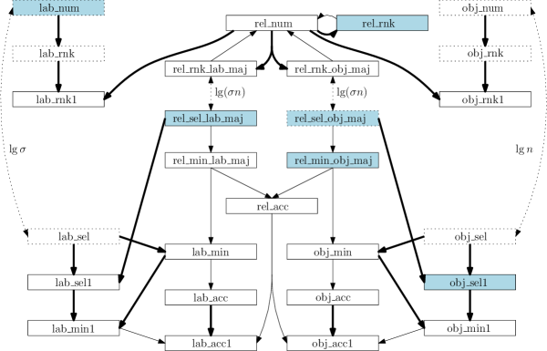
Figure 5: Reductions among operations supported by BinRel-WT. The dotted boxes are operations supported in $\omega(\lg\sigma)$ time, the filled boxes represent operations directly addressed in the paper, and the blank boxes are supported via reductions.

6 Using a Generalized Wavelet Tree: BinRel-GWT

The results we obtained for the wavelet tree can be extended to the generalized wavelet tree, improving complexities in many cases (recall Section 2.3). We refer to the structure that represents $S$ using the generalized wavelet tree as BinRel-GWT, and we use $\mu$ to represent the fan-out of the tree. We require $\mu\in O(\lg^{\epsilon}(n\sigma))$, assuming that the RAM machine can address up to $n\times\sigma$ cells. To simplify we will assume $\sigma\leq n$ and then use simply $\mu\in O(\lg^{\epsilon}n)$.

A first simple result stems from the fact that the string operations are sped up on generalized wavelet trees.

Lemma 7.

BinRel-GWT supports $\mathtt{obj\_rnk1}$ and $\mathtt{obj\_sel1}$ in time $O(\lg_{\mu}\sigma)$ for any $\mu\in\Theta(\lg^{\epsilon}n)$ and any constant $0<\epsilon<1$.

Proof.

This follows directly from the results on general BinRel-Str structures. ∎

The following notation will be useful to describe our algorithms within wavelet tree nodes. Note that all are easily computed in constant time.

• $\mathtt{child}(k)$: Given a symbol $k\in[1,\mu]$, this is the subtree labeled $k$ of the current node.

• $\mathtt{g}(\alpha)$: Given a symbol $\alpha\in[1,\sigma]$, $\mathtt{g}(\alpha)$ is the symbol $k$ such that $\mathtt{child}(k)$ contains the leaf corresponding to $\alpha$.

• $\mathtt{g}^{-1}(k)$: Given a symbol $k\in[1,\mu]$, $\mathtt{g}^{-1}(k)=\min\{\alpha,k=\mathtt{g}(\alpha)\}$.

The next lemma shows how to speed up all the range counting operations. The result is known in the literature for $n\times n$ grids, even within $n\lg n(1+o(1))$ bits of space [10].

Lemma 8.

BinRel-GWT supports $\mathtt{rel\_rnk}(\alpha,x)$ in $O(\lg_{\mu}\sigma)$ time, for any $\mu\in\Theta(\lg^{\epsilon}n)$ and any constant $0<\epsilon<1$.

Proof.

As in the case of BinRel-WT, we reduce this problem to the one of computing $\mathtt{rank}_{\leq\alpha}(S,\mathtt{map}(x))$, which can be done by following a similar procedure: We follow the path for $\alpha$ starting at the root in position $p=\mathtt{map}(x)$ and with a counter $c\leftarrow 0$. Every time we move to a subtree, we increase $c\leftarrow c+\mathtt{rank}_{\leq g(\alpha)-1}(S_{v},p)$. When we arrive at the leaf, the answer is $c+p$.

Operation $\mathtt{rank}_{\leq k}(S_{v},p)$ can be solved in constant time for $\mu\in\Theta(\lg^{\epsilon}n)$ analogously as done for $\mathtt{rank}_{k}$ on small alphabets (recall Section 2.2). We store for each $k\in[1,\mu]$ a bitmap $B_{\leq k}$ such that $B_{\leq k}[i]=1$ iff $S_{v}[i]\leq k$. Thus $\mathtt{rank}_{\leq k}(S_{v},p)=\mathtt{rank}_{1}(B_{\leq k},p)$ is computed in constant time and the whole process takes $O(\lg_{\mu}\sigma)$ time. ∎

The next lemma covers operation $\mathtt{rel\_sel\_lab\_maj}$, on which we cannot improve upon the complexity given by BinRel-WT. Note this means that $O(\lg\sigma)$ is still the best time complexity for supporting range_quantile queries within linear space [20].

Lemma 9.

BinRel-GWT supports $\mathtt{rel\_sel\_lab\_maj}(\alpha,j,x,y)$ in $O(\lg\sigma)$ time.

Proof.

This is solved in a similar way to the one presented for BinRel-WT. We find $v$ such that $\mathtt{rank}_{\leq\beta-1}(S,p,q)<v\leq\mathtt{rank}_{\leq\beta}(S,p,q)$. The only difference is that in this case we have to do, at each node, a binary search for the right child $k\in[1,\mu]$ to descend, and thus the time is $O(\lg\mu\lg_{\mu}\sigma)=O(\lg\sigma)$. ∎

For the next operations we will augment the generalized wavelet tree with a set of bitmaps inside each node $v$. More specifically, we will add $\mu(\mu+1)/2$ bitmaps $B_{k,l}$, where $B_{k,l}[i]=1$ iff $S_{v}[i]\in[k,l]$. Just as bitmaps $B_{\leq k}$, bitmaps $B_{k,l}$ are not represented explicitly, but only their index is stored (recall Section 2.2), and their content is simulated in constant time using $S_{v}$. Their total space for a sequence $S_{v}[1,n]$ is $O(n\mu^{2}\lg\lg n/\lg_{\mu}n)$. To make this space negligible, that is, $o(n\lg\mu)$, it is sufficient that $\mu=O(\lg^{\epsilon}n)$ for any constant $0<\epsilon<1/2$. (A related idea has been used by Farzan et al. [17].)

The next lemma shows that the current solution for operation prevLess [26] can be sped up by an $O(\lg\lg n)$ factor.

Lemma 10.

BinRel-GWT supports $\mathtt{rel\_min\_obj\_maj}(\alpha,\beta,\gamma,x)$ in $O(\lg_{\mu}\sigma)$ time, for any $\mu\in\Theta(\lg^{\epsilon}n)$ and any constant $0<\epsilon<1/2$.

Proof.

We first run query $\mathtt{rel\_min\_obj\_maj}(\gamma,\beta,\gamma,x)$, and if the result is on column $x$, we report it. Otherwise we run query $\mathtt{rel\_min\_obj\_maj}(\alpha,\beta,\alpha,x+1)$. This means that we can focus on a simpler query of the form $\mathtt{rel\_min\_obj\_maj}(\alpha,\beta,x)$, which finds the first pair in $[\alpha,\beta]\times[x,n]$, in object-major order. We map $[x,n]$ to $S[p,t]$ as usual and then proceed recursively on the wavelet tree, remapping $p$. At each node $v$, we decompose the query into three subqueries, and then take the minimum result of the three:

1. $\mathtt{rel\_min\_obj\_maj}(\alpha,\mathtt{g}^{-1}(\mathtt{g}(\alpha)+1)-1,x)$ on node $\mathtt{child}(\alpha)$;

2. $\mathtt{rel\_min\_obj\_maj}(\mathtt{g}^{-1}(\mathtt{g}(\alpha)+1),\mathtt{g}^{-1}(\mathtt{g}(\beta))-1,x)$ on the same node $v$;

3. $\mathtt{rel\_min\_obj\_maj}(\mathtt{g}^{-1}(\mathtt{g}(\beta)),\beta,x)$ on node $\mathtt{child}(\beta)$.

Note that queries of type 1 will generate, recursively, only $O(\lg_{\mu}\sigma)$ further queries of type 1 and 2, and similarly queries of type 3 will generate $O(\lg_{\mu}\sigma)$ further queries of type 3 and 2. The only queries that actually deliver values are those of type 2, and we will have to take the minimum over $O(\lg_{\mu}\sigma)$ such results.

A query of type 2 is solved in constant time using bitmap $B_{\mathtt{g}(\alpha)+1,\mathtt{g}(\beta)-1}$, by computing $q=\mathtt{select}_{1}(B_{\mathtt{g}(\alpha)+1,\mathtt{g}(\beta)-1},\mathtt{rank}_{1}(B_{\mathtt{g}(\alpha)+1,\mathtt{g}(\beta)-1},p-1)+1)$. This returns a position $S_{v}[q]$. As we return from the recursion, we remap $q$ in its parent in the usual way, and then (possibly) compare $q$ with the result of a query of type 1 or 3 carried out on the parent. We keep the minimum $q$ value along the way, and when we arrive at the root we return $(S[q],\mathtt{unmap}(q))$. ∎

For the next lemma we need a further data structure. For each sequence $S_{v}[1,n]$, we store an RMQ structure (Section 2.4), using $O(n)=o(n\lg\mu)$ bits and finding in constant time position of a minimum symbol in any range $S_{v}[i,j]$. This results improves upon the result for query range_next_value [20].

Lemma 11.

BinRel-GWT supports $\mathtt{rel\_min\_lab\_maj}(\alpha,x,y,z)$ in $O(\lg_{\mu}\sigma+\lg\mu)$ time, for any $\mu\in\Theta(\lg^{\epsilon}n)$ and any constant $0<\epsilon<1$.

Proof.

Again, we can focus on a simpler query $\mathtt{rel\_min\_lab\_maj}(\alpha,x,y)$. We map $[x,y]$ to $S[p,q]$ as usual, and the goal is to find the leftmost minimum symbol in $S[p,q]$ that is larger than $\alpha$.

Assume we are in a wavelet tree node $v$ and the current interval of interest is $S_{v}[p,q]$. Then, if $S_{v}[p,q]$ contains symbol $\mathtt{g}(\alpha)$ (which is known in constant time with $\mathtt{rank}_{\mathtt{g}(\alpha)}(S_{v},p,q)>0$), we have to consider it first, by querying recursively the child labeled $\mathtt{g}(\alpha)$. If this recursive call returns an answer $p^{\prime}$, we return it in turn, remapping it to the parent node. If it does not, then any symbol larger than $\alpha$ in the range must correspond to a symbol strictly larger than $\mathtt{g}(\alpha)$ in $S_{v}[p,q]$. We check in constant time whether there is any value larger than $\mathtt{g}(\alpha)$ in $S_{v}[p,q]$, using $\mathtt{rank}_{\leq\mathtt{g}(\alpha)}(S_{v},p,q)<q-p+1$. If there is none, we return in turn with no answer.

If there is an answer, we binary search for the smallest $k\in[\mathtt{g}(\alpha)+1,\mu]$ such that $\mathtt{rank}_{\leq k}(S_{v},p,q)>\mathtt{rank}_{\leq\mathtt{g}(\alpha)}(S_{v},p,q)$. This binary search takes $O(\lg\mu)$ time and is done only once along the whole process. Once we identify the right $k$, we descend to the appropriate child and start the final stage of the process.

The final stage starts at a node where all the local symbols represent original symbols that are larger than $\alpha$, and therefore we simply look for the position $m=\textsc{rmq}(S_{v},p,q)$, which gives us, in constant time, the first occurrence of the minimum symbol in $S_{v}$, and descend to child $S[m]$. This is done until reaching a leaf, from where we return to the root, at position $p^{\prime}$, and return $(S[p^{\prime}],\mathtt{unmap}(p^{\prime}))$. It is easy to see that we work $O(1)$ time on $O(\lg_{\mu}\sigma)$ nodes and $O(\lg\mu)$ once. ∎

Lemma 12.

BinRel-GWT supports $\mathtt{rel\_sel\_obj\_maj}(\alpha,\beta,x,j)$ in $O(\min(\lg n,\lg j\lg(\beta-\alpha+1))\lg_{\mu}\sigma)$ time, for any $\mu\in\Theta(\lg^{\epsilon}n)$ and any constant $0<\epsilon<1/2$.

Proof.

The complexities are obtained the same way as for BinRel-WT. The binary search over $\mathtt{rel\_num}$ is sped up because BinRel-GWT supports this operation faster. The other complexity is in principle higher, because the interval $[\alpha,\beta]$ is split into as much as $O(\mu\lg(\beta-\alpha+1))$ nodes. However, this can be brought down again to $O(\lg(\beta-\alpha+1))$ by using the parent node $v$ of each group of (up to $\mu$) contiguous leaves $[k,l]$, and using $\mathtt{select}_{1}$ on the bitmaps $B_{k,l}$ of those parent nodes in order to simulate a contiguous range with all the values in $[k,l]$. So we still have $O(\lg(\beta-\alpha+1))$ binary searches of $O(\lg j)$ steps, and now each step costs $O(\lg_{\mu}\sigma)$. ∎

Lemma 13.

BinRel-GWT supports $\mathtt{lab\_num}(\alpha,\beta,x,y)$ in $O(\beta-\alpha+\lg_{\mu}\sigma)$ time, for any $\mu\in\Theta(\lg^{\epsilon}n)$ and any constant $0<\epsilon<1/2$.

Proof.

We follow the same procedure as for BinRel-WT. The main difference is how to compute the nodes covering the range $[\alpha,\beta]$. This can be done in a naïve way by just verifying whether each symbol appears in the range of $S_{v}$, but this raises the complexity by a factor of $\mu$. Thus we need a method to list the symbols appearing in a range of $S_{v}$ without probing non-existent ones. We resort to a technique loosely inspired by Muthukrishnan [29]. To list the symbol from a range $[k,l]$ that exist in $S_{v}[p,q]$, we start with the first symbol of the range that appears in $S_{v}[p,q]$. This is obtained with $p^{\prime}=\mathtt{select}_{1}(B_{k,l},\mathtt{rank}_{1}(B_{k,l},p-1)+1)$. If $p^{\prime}>q$ then there are no such symbols. Otherwise, let $k^{\prime}=S_{v}[p^{\prime}]$. Then we know that $k^{\prime}$ appears in $S_{v}[p,q]$. Now we continue recursively with subranges $[k,k^{\prime}-1]$ and $[k^{\prime}+1,l]$. The recursion stops when no $p^{\prime}$ is found, and it yields all the symbols appearing in $S_{v}[p,q]$ in $O(1)$ time per symbol. ∎

The remaining operations are obtained by brute force, just as with BinRel-WT. Figure 6 illustrates the reductions used.

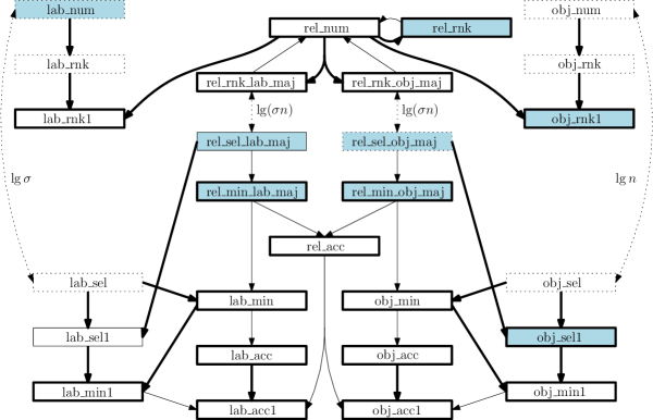
Figure 6: Reductions among operations supported by BinRel-GWT. The dotted boxes are operations supported in $\omega(\lg\sigma)$ time, the solid ones in $O(\lg\sigma)$ time, and the thick ones in time $O(\lg_{\mu}\sigma)$ or $O(\lg_{\mu}\sigma+\lg\mu)$. The filled boxes represent operations addressed directly, and the blank boxes are supported via reductions.

Theorem 3.

The structure BinRel-GWT, for a binary relation $\mathcal{R}$ of $t$ pairs over $[1,\sigma]\times[1,n]$, requires $t\lg\sigma(1+o(1))+O(n+t)$ bits of space and supports the operations within the time complexities given in Table 2.

Operation	BinRel-GWT	BinRel-WT
$\mathtt{rel\_num}(\alpha,\beta,x,y)$	$O(\lg\sigma/\lg\lg n)$	$O(\lg\sigma)$
$\mathtt{rel\_rnk}(\alpha,x)$	$O(\lg\sigma/\lg\lg n)$	$O(\lg\sigma)$
$\mathtt{rel\_rnk\_lab\_maj}(\alpha,x,y,z)$	$O(\lg\sigma/\lg\lg n)$	$O(\lg\sigma)$
$\mathtt{rel\_sel\_lab\_maj}(\alpha,j,x,y)$	$O(\lg\sigma)$	$O(\lg\sigma)$
$\mathtt{rel\_min\_lab\_maj}(\alpha,x,y,z)$	$O(\lg\sigma/\lg\lg n+\lg\lg n)$	$O(\lg\sigma)$
$\mathtt{rel\_rnk\_obj\_maj}(\alpha,\beta,\gamma,x)$	$O(\lg\sigma/\lg\lg n)$	$O(\lg\sigma)$
$\mathtt{rel\_sel\_obj\_maj}(\alpha,\beta,x,j)$	$O(\lg j\lg(\beta-\alpha+1)\lg\sigma/\lg\lg n)$ $O(\lg n\lg\sigma/\lg\lg n)$	$O(\lg j\lg(\beta-\alpha+1)\lg\sigma)$ $O(\lg n\lg\sigma)$
$\mathtt{rel\_min\_obj\_maj}(\alpha,\beta,\gamma,x)$	$O(\lg\sigma/\lg\lg n)$	$O(\lg\sigma)$
$\mathtt{rel\_acc}(\alpha,\beta,x,y)$	$O((k+1)\lg\sigma/\lg\lg n)$	$O((k+1)\lg\sigma)$
$\mathtt{lab\_num}(\alpha,\beta,x,y)$	$O(\beta-\alpha+\lg\sigma/\lg\lg n)$	$O(\beta-\alpha+\lg\sigma)$
$\mathtt{lab\_rnk}(\alpha,x,y)$	$O(\alpha+\lg\sigma/\lg\lg n)$	$O(\alpha+\lg\sigma)$
$\mathtt{lab\_sel}(\alpha,j,x,y)$	$O(j(\lg\sigma/\lg\lg n+\lg\lg n))$	$O(j\lg\sigma)$
$\mathtt{lab\_acc}(\alpha,x,y)$	$O((k+1)(\lg\sigma/\lg\lg n+\lg\lg n))$	$O((k+1)\lg\sigma)$
$\mathtt{lab\_min}(\alpha,x,y)$	$O(\lg\sigma/\lg\lg n+\lg\lg n)$	$O(\lg\sigma)$
$\mathtt{obj\_num}(\alpha,\beta,x,y)$	$O((y-x+1)\lg\sigma/\lg\lg n)$	$O((y-x+1)\lg\sigma)$
$\mathtt{obj\_rnk}(\alpha,\beta,x)$	$O((y-x+1)\lg\sigma/\lg\lg n)$	$O((y-x+1)\lg\sigma)$
$\mathtt{obj\_sel}(\alpha,\beta,x,j)$	$O(j\lg\sigma/\lg\lg n)$	$O(j\lg\sigma)$
$\mathtt{obj\_acc}(\alpha,\beta,x)$	$O((k+1)\lg\sigma/\lg\lg n)$	$O((k+1)\lg\sigma)$
$\mathtt{obj\_min}(\alpha,\beta,x)$	$O(\lg\sigma/\lg\lg n)$	$O(\lg\sigma)$
$\mathtt{lab\_rnk1}(\alpha,x)$	$O(\lg\sigma/\lg\lg n)$	$O(\lg\sigma)$
$\mathtt{lab\_sel1}(\alpha,j,x)$	$O(\lg\sigma)$	$O(\lg\sigma)$
$\mathtt{lab\_min1}(\alpha,j,x)$	$O(\lg\sigma/\lg\lg n+\lg\lg n)$	$O(\lg\sigma)$
$\mathtt{lab\_acc1}(\alpha,j,x)$	$O((k+1)\lg\sigma/\lg\lg n)$	$O((k+1)\lg\sigma)$
$\mathtt{obj\_rnk1}(\alpha,x)$	$O(\lg\sigma/\lg\lg n)$	$O(\lg\sigma)$
$\mathtt{obj\_sel1}(\alpha,x,j)$	$O(\lg\sigma/\lg\lg n)$	$O(\lg\sigma)$
$\mathtt{obj\_min1}(\alpha,x,j)$	$O(\lg\sigma/\lg\lg n)$	$O(\lg\sigma)$
$\mathtt{obj\_acc1}(\alpha,x,j)$	$O((k+1)\lg\sigma/\lg\lg n)$	$O((k+1)\lg\sigma)$

Table 2: Time complexity for the operations for BinRel-GWT and BinRel-WT. The parameter $k$ represents the size of the output for the $\mathtt{access}$ operators; one can consider $k=1$ for the reductions shown in Theorem 1.

7 Binary Relation Wavelet Trees (BRWT)

We propose now a special wavelet tree structure tailored to the representation of binary relations. This wavelet tree contains two bitmaps per level at each node $v$, $B_{v}^{l}$ and $B_{v}^{r}$. At the root, $B_{v}^{l}[1,n]$ has the $x$-th bit set to $1$ iff there exists a pair $(\alpha,x)$ with $\alpha\in[1,\lfloor\sigma/2\rfloor]$, and $B_{v}^{r}$ has the $x$-th bit set to $1$ iff there exists a pair $(\alpha,x)$ with $\alpha\in[\lfloor\sigma/2\rfloor+1,\sigma]$. Left and right subtrees are recursively built on the positions set to $1$ in $B_{v}^{l}$ and $B_{v}^{r}$, respectively. The leaves (where no bitmap is stored) correspond to individual rows of the relation. We store a bitmap $B[1,\sigma+t]$ recording in unary the number of elements in each row. See Figure 7 for an example. For ease of notation, we define the following functions on $B$, trivially supported in constant-time: $\mathtt{lab}(r)=1+\mathtt{rank}_{0}(B,\mathtt{select}_{1}(B,r))$ gives the label of the $r$-th pair in a label-major traversal of $R$; while its inverse $\mathtt{poslab}(\alpha)=\mathtt{rank}_{1}(B,\mathtt{select}_{0}(B,\alpha))$ gives the position in the traversal where the pairs for label $\alpha$ start.

Figure 7: Example of the BRWT for the binary relation in Figure 1.

Note that, because an object $x$ may propagate both left and right, the sizes of the second-level bitmaps may add up to more than $n$ bits. Indeed, the last level contains $t$ bits and represents all the pairs sorted in row-major order. As we will see, the BRWT has weaker functionality than our former structures based on wavelet trees, but it reaches space proportional to $H(\mathcal{R})$.

Lemmas 14 to 18 give a set of operations that can be supported with the BRWT structure.

Lemma 14.

BRWT supports $\mathtt{rel\_num}(\alpha,\beta,x,y)$ in $O(\beta-\alpha+\lg\sigma)$ time.

Proof.

We project the interval $[x,y]$ from the root to each leaf in $[\alpha,\beta]$, adding up the resulting interval sizes at the leaves. Of course we can stop earlier if the interval becomes empty. Note that we can only count pairs at the leaves, not at internal nodes. ∎

Lemma 15.

BRWT supports $\mathtt{rel\_min\_lab\_maj}(\alpha,x,y,z)$ in $O(\lg\sigma)$ time.

Proof.

As before, we only need to consider the simpler query $\mathtt{rel\_min\_lab\_maj}(\alpha,x,y)$. We reach the $O(\lg\sigma)$ wavelet tree nodes $v_{1},v_{2},\ldots$ that cover the interval $[\alpha,\sigma]$, and map $[x,y]$ to all those nodes, in $O(\lg\sigma)$ time [20]. We choose the first such node, $v_{k}$, left to right, with a nonempty interval $[x,y]$. Now we find the leftmost leaf of $v_{k}$ that has a nonempty interval $[x,y]$, which is easily done in $O(\lg\sigma)$ time. Once we arrive at such a leaf $\gamma$ with interval $[x,y]$, we map $x$ back to the root, obtaining $x^{\prime}$, and the answer is $(\gamma,x^{\prime})$. ∎

Lemma 16.

BRWT supports $\mathtt{rel\_min\_obj\_maj}(\alpha,\beta,\gamma,x)$ in $O(\lg\sigma)$ time.

Proof.

As before, we only need to consider the simpler query $\mathtt{rel\_min\_obj\_maj}(\alpha,\beta,x)$. Analogously to the proof of Lemma 4, we cover $[\alpha,\beta]$ with $O(\lg\sigma)$ wavelet tree nodes $v_{1},v_{2},\dots$, and map $x$ to $x_{i}$ at each such $v_{i}$, all in $O(\lg\sigma)$ time. Now, on the way back of this recursion, we obtain the smallest $y\geq x$ in the root associated to some label in $[\alpha,\beta]$. In this process we keep track of the node $v_{i}$ that is the source of $y$, preferring the left child in case of ties. Finally, if we arrive at the root with a value $y$ that came from node $v_{i}$, we start from position $x^{\prime}=x_{i}$ at node $v_{i}$ and find the leftmost leaf of $v_{i}$ related to $y$. This is done by going left whenever possible (i.e., if $B_{v}^{l}[x^{\prime}]=1$) and right otherwise, and remapping $x^{\prime}$ appropriately at each step. Upon reaching a leaf $\gamma$, we report $(\gamma,y)$. ∎

Lemma 17.

BRWT supports $\mathtt{obj\_sel1}(\alpha,x,j)$ in $O(\lg\sigma)$ time.

Proof.

We map $x-1$ from the root to $x^{\prime}$ in leaf $\alpha$, then walk upwards the path from $x^{\prime}+j$ to the root and report the position obtained. ∎

Lemma 18.

BRWT supports $\mathtt{lab\_num}(\alpha,\beta,x,y)$ in $O(\beta-\alpha+\lg\sigma)$ time.

Proof.

We map $[x,y]$ from the root to each leaf in $[\alpha,\beta]$, adding one per leaf where the interval is non-empty. Recursion can also stop when $[x,y]$ becomes empty. ∎

The remaining complexities are obtained by brute force: $\mathtt{rel\_sel\_lab\_maj}$ and $\mathtt{rel\_sel\_obj\_maj}$ are obtained by iterating with $\mathtt{rel\_min\_lab\_maj}$ and $\mathtt{rel\_min\_obj\_maj}$, respectively; and similarly $\mathtt{lab\_sel}$, $\mathtt{obj\_sel}$ and $\mathtt{lab\_sel1}$ using $\mathtt{lab\_min}$, $\mathtt{obj\_min}$, and $\mathtt{lab\_min1}$. Finally, as before $\mathtt{obj\_num}$ and $\mathtt{obj\_rnk}$ are obtained by iterating over $\mathtt{obj\_rnk1}$. We have obtained the following theorem, illustrated in Figure 8.

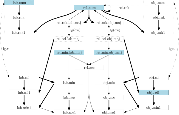
Figure 8: Reductions among operations supported by BRWT. The dotted boxes are operations supported in $\omega(\lg\sigma)$ time, the filled boxes represent operations directly addressed in the paper, and the blank boxes are supported via reductions.

Theorem 4.

The BRWT structure, for a binary relation $\mathcal{R}$ of $t$ pairs over $[1,\sigma]\times[1,n]$, uses $\lg(1+\sqrt{2})H(\mathcal{R})+O(t+n+\sigma)$ bits of space and supports the operations within the complexities given in Table 3.

Proof.

The operations have been obtained throughout the section. For the space, $B$ is of length $\sigma+t$. Thus $O(t+n+\sigma)$ bits account for $B$ and for the $2n$ bits at the root of the wavelet tree. The rest of the bits in the wavelet tree can be counted by considering that each bit not in the root is induced by the presence of a pair.

Each pair has a unique representative bit in a leaf, and also induces the presence of bits up to the root. Yet those leaf-to-root paths get merged, so that not all those bits are different. Consider an element $x$ related to $t_{x}$ labels. It induces $t_{x}$ bits at $t_{x}$ leaves, and each such bit at a leaf induces a bit per level on a path from the leaf towards the single $x$ at the root. At worst, all the $O(t_{x})$ bits up to level $\lg t_{x}$ are created for these elements, and from there on all the $t_{x}$ paths are different, adding up a total of $O(t_{x})+t_{x}\lg\frac{\sigma}{t_{x}}$ bits. Adding over all $x$ we get $O(t)+\sum_{x}t_{x}\lg\frac{\sigma}{t_{x}}$. This is maximized when $t_{x}=t/n$ for all $x$, yielding $O(t)+t\lg\frac{\sigma n}{t}=H(\mathcal{R})+O(t)$ bits.

Instead of representing two bitmaps (which would multiply the above value by 2), we can represent a single sequence $B_{v}$ with the possible values of the two bits at each position, 00, 01, 10, 11. Only at the root is 00 possible. Except for those $2n$ bits, we can represent the sequence over an alphabet of size 3 with a zero-order representation [23], to achieve at worst $(\lg 3)H(\mathcal{R})+o(t)$ bits for this part while retaining constant-time $\mathtt{rank}$ and $\mathtt{select}$ over each $B_{v}^{l}$ and $B_{v}^{r}$. (To achieve this, we maintain the directories for the original bitmaps, of sublinear size.)

To improve the constant $\lg 3$ to $\lg(1+\sqrt{2})$, we consider that the zero-order representation actually achieves $|B_{v}|H_{0}(B_{v})$ bits. We call $B_{x}$ the concatenation of all the symbols induced by $x$, $\ell_{x}=|B_{x}|\leq t_{x}$, and $H_{x}=|B_{x}|H_{0}(B_{x})$. Assume the $t_{x}$ bits are partitioned into $t_{01}$ 01’s, $t_{10}$ 10’s, and $t_{11}$ 11’s, so that $t_{x}=t_{01}+t_{10}+2t_{11}$, $\ell_{x}=t_{01}+t_{10}+t_{11}$, and $H_{x}=t_{01}\lg\frac{\ell_{x}}{t_{01}}+t_{10}\lg\frac{\ell_{x}}{t_{10}}+t_{11}\lg\frac{\ell_{x}}{t_{11}}$. As $t_{11}=(t_{x}-t_{01}-t_{10})/2$, the maximum of $H_{x}$ as a function of $t_{01}$ and $t_{10}$ yields the worst case at $t_{01}=t_{10}=\frac{\sqrt{2}}{4}t_{x}$, so $t_{11}=(\frac{1}{2}-\frac{\sqrt{2}}{4})t_{x}$ and $\ell_{x}=(\frac{1}{2}+\frac{\sqrt{2}}{4})t_{x}$, where $H_{x}=\lg(1+\sqrt{2})t_{x}$ bits. This can be achieved separately for each symbol. Using the same distribution of 01’s, 10’s, and 11’s for all $x$ we add up to $\lg(1+\sqrt{2})t\lg\frac{\sigma n}{t}+O(t)=\lg(1+\sqrt{2})H(\mathcal{R})+O(t)$ bits. (Note that, if we concatenate all the wavelet tree levels, the $H_{x}$ strings are interleaved in this concatenation.) ∎

Note that this is a factor of $\lg(1+\sqrt{2})\approx 1.272$ away of the entropy of $\mathcal{R}$.

Operation	BRWT	BinRel-WT
$\mathtt{rel\_num}(\alpha,\beta,x,y)$	$O(\beta-\alpha+\lg\sigma)$	$O(\lg\sigma)$
$\mathtt{rel\_rnk}(\alpha,x)$	$O(\alpha+\lg\sigma)$	$O(\lg\sigma)$
$\mathtt{rel\_rnk\_lab\_maj}(\alpha,x,y,z)$	$O(\alpha+\lg\sigma)$	$O(\lg\sigma)$
$\mathtt{rel\_sel\_lab\_maj}(\alpha,j,x,y)$	$O(j\lg\sigma)$	$O(\lg\sigma)$
$\mathtt{rel\_min\_lab\_maj}(\alpha,x,y,z)$	$O(\lg\sigma)$	$O(\lg\sigma)$
$\mathtt{rel\_rnk\_obj\_maj}(\alpha,\beta,\gamma,x)$	$O(\beta-\alpha+\lg\sigma)$	$O(\lg\sigma)$
$\mathtt{rel\_sel\_obj\_maj}(\alpha,\beta,x,j)$	$O(j\lg\sigma)$	$O(\lg j\lg(\beta-\alpha+1)\lg\sigma)$ $O(\lg n\lg\sigma)$
$\mathtt{rel\_acc}(\alpha,\beta,x,y)$	$O((k+1)\lg\sigma)$	$O((k+1)\lg\sigma)$
$\mathtt{rel\_min\_obj\_maj}(\alpha,\beta,\gamma,x)$	$O(\lg\sigma)$	$O(\lg\sigma)$
$\mathtt{lab\_num}(\alpha,\beta,x,y)$	$O(\beta-\alpha+\lg\sigma)$	$O(\beta-\alpha+\lg\sigma)$
$\mathtt{lab\_rnk}(\alpha,x,y)$	$O(\alpha+\lg\sigma)$	$O(\alpha+\lg\sigma)$
$\mathtt{lab\_sel}(\alpha,j,x,y)$	$O(j\lg\sigma)$	$O(j\lg\sigma)$
$\mathtt{lab\_acc}(\alpha,x,y)$	$O((k+1)\lg\sigma)$	$O((k+1)\lg\sigma)$
$\mathtt{lab\_min}(\alpha,x,y)$	$O(\lg\sigma)$	$O(\lg\sigma)$
$\mathtt{obj\_num}(\alpha,\beta,x,y)$	$O((y-x+1)\lg\sigma)$	$O((y-x+1)\lg\sigma)$
$\mathtt{obj\_rnk}(\alpha,\beta,x)$	$O((y-x+1)\lg\sigma)$	$O((y-x+1)\lg\sigma)$
$\mathtt{obj\_sel}(\alpha,\beta,x,j)$	$O(j\lg\sigma)$	$O(j\lg\sigma)$
$\mathtt{obj\_acc}(\alpha,\beta,x)$	$O((k+1)\lg\sigma)$	$O((k+1)\lg\sigma)$
$\mathtt{obj\_min}(\alpha,\beta,x)$	$O(\lg\sigma)$	$O(\lg\sigma)$
$\mathtt{lab\_rnk1}(\alpha,x)$	$O(\lg\sigma)$	$O(\lg\sigma)$
$\mathtt{lab\_sel1}(\alpha,j,x)$	$O(j\lg\sigma)$	$O(\lg\sigma)$
$\mathtt{lab\_min1}(\alpha,j,x)$	$O(\lg\sigma)$	$O(\lg\sigma)$
$\mathtt{lab\_acc1}(\alpha,j,x)$	$O((k+1)\lg\sigma)$	$O((k+1)\lg\sigma)$
$\mathtt{obj\_rnk1}(\alpha,x)$	$O(\lg\sigma)$	$O(\lg\sigma)$
$\mathtt{obj\_sel1}(\alpha,x,j)$	$O(\lg\sigma)$	$O(\lg\sigma)$
$\mathtt{obj\_min1}(\alpha,x,j)$	$O(\lg\sigma)$	$O(\lg\sigma)$
$\mathtt{obj\_acc1}(\alpha,x,j)$	$O((k+1)\lg\sigma)$	$O((k+1)\lg\sigma)$

Table 3: Time complexity for the operations for BRWT and BinRel-WT. The parameter $k$ represents the size of the output for the $\mathtt{access}$ operators; one can consider $k=1$ for the reductions shown in Theorem 1.

8 Conclusions and Future Work

Motivated by the many applications where a binary relation $\mathcal{R}$ between $\sigma$ labels and $n$ objects arises, we have proposed a rich set of primitives of interest in such applications. We first extended existing representations and showed that their potential is very limited outside single-row or single-column operations. Then we proposed a representation called BinRel-WT, that uses a wavelet tree to solve a large number of operations in time $O(\lg\sigma)$. This structure has been already of use in particular cases, but here we have made systematic use of it and exposed its full potential. Furthermore, we have extended the results to generalized wavelet trees, to obtain the structure BinRel-GWT. This structure achieves $O(\lg\sigma/\lg\lg n)$ time for many operations. It had already been used for range counting and reporting [10], but here we have extended its functionality to many other operations, so that its use as a replacement of the better known BinRel-WT structure improves the times achieved in various applications by a $\lg\lg n$ factor.

Some of those speedups have already been mentioned in the article, namely operations range_next_value and prevLess [20, 26] (range_quantile, on the other hand, is an interesting operation that has resisted our attempts to improve it; it is equivalent to $\mathtt{rel\_sel\_lab\_maj}$). Another example is finding the dominant points on a grid, that is, those $(x,y)$ so that there is not another $(x^{\prime},y^{\prime})$ with $x^{\prime}\leq x$ and $y^{\prime}\leq y$. Using successive calls to $\mathtt{rel\_min\_obj\_maj}$ and restricting the next call to the area $[x+1,n]\times[1,y-1]$ where $(x,y)$ is the last pair found, structure BinRel-GWT can find the dominant points in time $O(\lg n/\lg\lg n)$ per point, on an $n\times n$ grid. This improves upon the $O(\lg n)$ time achieved in the literature [30].

The speedup on counting and reporting on grids is useful in various text indexing data structures. As an example, Arroyuelo et al. [1] describe a Lempel-Ziv compressed index that is able to find the $occ$ occurrences of a pattern of length $m$ in a text $T[1,n]$ in time $O(m^{2}+(m+occ)\lg n)$. For this sake they use a 2-dimensional grid where $O(m)$ $\mathtt{rel\_rnk}$ and $O(occ)$ $\mathtt{rel\_acc}$ operations are carried out. By using our new BinRel-GWT structure, their time complexity drops to $O(m^{2}+(m+occ)\lg n/\lg\lg n)$. As a second example, Claude and Navarro [16] use grammar-based compression to solve the same problem. Given a grammar of $n$ rules and height $h$, they achieve search time $O(m(m+h)+h\,occ)\lg n)$. They use a 2-dimensional grid where operations $\mathtt{rel\_acc}$, $\mathtt{lab\_sel1}$, and $\mathtt{obj\_sel1}$ are carried out, and therefore using a BinRel-GWT structure their time is reduced to $O(m(m+h)+h\,occ)\lg n/\lg\lg n)$.

Despite the fact that our structures solve many of the queries we have proposed in polylogarithmic (and usually logarithmic) time, supporting others remains a challenge. In particular, we have no good solutions for label-level or object-level $\mathtt{rank}$ and $\mathtt{select}$ queries on ranges.

Another challenge is space. All of the described structures use essentially $t\lg\sigma$ bits of space, where $t$ is the number of pairs in the relation. While this is reasonable in many cases, it can be far from the entropy of the binary relation, $H(\mathcal{R})$, for dense relations. We have proposed a variant, BRWT, that uses space within a multiplicative factor 1.272 of $H(\mathcal{R})$, yet its functionality is more limited: Apart from label-level and object-level queries, this structure does not support to efficiently count and select arbitrary points in ranges, albeit it can efficiently enumerate them.

Since the publication of the conference version of this article [3], a followup work [17] used our representation BinStr-WT as an internal structure to achieve asymptotically optimum space, $H(\mathcal{R})+o(H(\mathcal{R}))$ bits, and was able to solve query $\mathtt{rel\_rnk}$ in time $O(\lg n)$, and queries $\mathtt{rel\_acc}$, $\mathtt{rel\_sel\_lab\_maj}$ and $\mathtt{rel\_sel\_obj\_maj}$ in time $O(\lg^{2}n)$, on $n\times n$ grids. Once again, using structure BinRel-GWT their times for $\mathtt{rel\_rnk}$ and $\mathtt{rel\_acc}$ can be divided by $\lg\lg n$.

It is therefore an open challenge to approach space $H(\mathcal{R})$ as much as possible while retaining the maximum possible functionality and the best possible efficiency. It is unclear which are the limits in this space/time tradeoff, although some lower bounds from computational geometry are useful. For example, we cannot count points in ranges faster than the BinRel-GWT structure within polylogarithmic space [31].

On the other hand, $H(\mathcal{R})$ is a crude measure that does not account for regularities in the row/column distribution, or clustering, that arises in real-life binary relations. For example, structures BinRel-WT and BinRel-GWT can be compressed to the zero-order entropy of a string of length $t$, and this can in some cases be below $H(\mathcal{R})$, which shows that this measure is not sufficiently refined. It would be interesting to consider finer measures of entropy and try to match them.

There might also be other operations of interest apart from the set we have identified. For example, determining whether a pair is related in the transitive closure of $\mathcal{R}$ is relevant for many applications (e.g., ancestorship in trees, or paths in graphs). Another extension is to $d$-ary relations, which would more naturally capture joins in the relational model.

Finally, we have considered only static relations. Our representations do allow dynamism, where new pairs and/or objects can be inserted in/deleted from the waveleet trees [28]. Adding/removing labels, instead, is an open challenge, as it alters the shape of the wavelet tree.

Appendix A Formal Definition of Operations

We formally define our set of operations. Figure 9 graphically illustrates some of them.

• $\mathtt{rel\_acc}(\alpha,\beta,x,y)~{}=~{}\{(\gamma,z)\in\mathcal{R},\ \gamma\in[\alpha,\beta]~{}\land~{}z\in[x,y]\}$

• $\mathtt{rel\_sel\_lab\_maj}(\alpha,j,x,y)~{}=~{}j\textrm{-th smallest pair of}~{}\mathtt{rel\_acc}(\alpha,\sigma,x,y)$ in order $(\alpha,x)\leq(\beta,y)\Leftrightarrow\alpha<\beta\lor(\alpha=\beta\land x\leq y)$

• $\mathtt{rel\_min\_lab\_maj}(\alpha,x,y,z)~{}=~{}\textrm{under the same order, smallest pair of}$ $\mathtt{rel\_acc}(\alpha,\alpha,z,y)\cup\mathtt{rel\_acc}(\alpha{+}1,\sigma,x,y)$

• $\mathtt{rel\_sel\_obj\_maj}(\alpha,\beta,x,j)~{}=~{}j\textrm{-th smallest pair of}~{}\mathtt{rel\_acc}(\alpha,\beta,x,n)$ in order $(\alpha,x)\leq(\beta,y)\Leftrightarrow x<y\lor(x=y\land\alpha\leq\beta)$

• $\mathtt{rel\_min\_obj\_maj}(\alpha,\beta,\gamma,x)~{}=~{}\textrm{under the same order, smallest pair of}$ $\mathtt{rel\_acc}(\gamma,\beta,x,x)\cup\mathtt{rel\_acc}(\alpha,\beta,x{+}1,n)$

• $\mathtt{lab\_acc}(\alpha,\beta,x,y)~{}=~{}\{\gamma,\ \exists z,\ (\gamma,z)\in\mathtt{rel\_acc}(\alpha,\beta,x,y)\}$

• $\mathtt{lab\_acc1}(\alpha,\beta,x)~{}=~{}\mathtt{lab\_acc}(\alpha,\beta,x,x)$

• $\mathtt{lab\_sel}(\alpha,j,x,y)~{}=~{}j\textrm{-th smallest label of}~{}\mathtt{lab\_acc}(\alpha,\sigma,x,y)$

• $\mathtt{lab\_sel1}(\alpha,j,x)~{}=~{}\mathtt{lab\_sel}(\alpha,j,x,x)$, or $\mathtt{rel\_sel\_lab\_maj}(\alpha,j,x,x)$

• $\mathtt{lab\_min}(\alpha,x,y)~{}=~{}\mathtt{lab\_sel}(\alpha,1,x,y)$

• $\mathtt{lab\_min1}(\alpha,x)~{}=~{}\mathtt{lab\_min}(\alpha,x,x)$, or $\mathtt{lab\_sel1}(\alpha,1,x)$

• $\mathtt{obj\_acc}(\alpha,\beta,x,y)~{}=~{}\{z,\ \exists\gamma,\ (\gamma,z)\in\mathtt{rel\_acc}(\alpha,\beta,x,y)\}$

• $\mathtt{obj\_acc1}(\alpha,x,y)~{}=~{}\mathtt{obj\_acc}(\alpha,\alpha,x,y)$

• $\mathtt{obj\_sel}(\alpha,\beta,x,j)~{}=~{}j\textrm{-th smallest object of}~{}\mathtt{obj\_acc}(\alpha,\beta,x,n)$

• $\mathtt{obj\_sel1}(\alpha,x,j)~{}=~{}\mathtt{obj\_sel}(\alpha,\alpha,x,j)$, or $\mathtt{rel\_sel\_obj\_maj}(\alpha,\alpha,x,j)$

• $\mathtt{obj\_min}(\alpha,\beta,x)~{}=~{}\mathtt{obj\_sel}(\alpha,\beta,x,1)$

• $\mathtt{obj\_min1}(\alpha,x)~{}=~{}\mathtt{obj\_min}(\alpha,\alpha,x)$, or $\mathtt{obj\_sel1}(\alpha,x,1)$

• $\mathtt{rel\_num}(\alpha,\beta,x,y)~{}=~{}|\mathtt{rel\_acc}(\alpha,\beta,x,y)|$

• $\mathtt{rel\_rnk}(\alpha,x)~{}=~{}\mathtt{rel\_num}(1,\alpha,1,x)$

• $\mathtt{rel\_rnk\_lab\_maj}(\alpha,x,y,z)~{}=~{}\mathtt{rel\_num}(1,\alpha{-}1,x,y){+}\mathtt{rel\_num}(\alpha,\alpha,x,z)$

• $\mathtt{rel\_rnk\_obj\_maj}(\alpha,\beta,\gamma,x)~{}=~{}\mathtt{rel\_num}(\alpha,\beta,1,x{-}1){+}\mathtt{rel\_num}(\alpha,\gamma,x,x)$

• $\mathtt{lab\_num}(\alpha,\beta,x,y)~{}=~{}|\mathtt{lab\_acc}(\alpha,\beta,x,y)|$

• $\mathtt{lab\_rnk}(\alpha,x,y)~{}=~{}\mathtt{lab\_num}(1,\alpha,x,y)$

• $\mathtt{lab\_rnk1}(\alpha,x)~{}=~{}\mathtt{lab\_rnk}(\alpha,x,x)$, or $\mathtt{rel\_num}(1,\alpha,x,x)$

• $\mathtt{obj\_num}(\alpha,\beta,x,y)~{}=~{}|\mathtt{obj\_acc}(\alpha,\beta,x,y)|$

• $\mathtt{obj\_rnk}(\alpha,\beta,x)~{}=~{}\mathtt{obj\_num}(\alpha,\beta,1,x)$

• $\mathtt{obj\_rnk1}(\alpha,x)~{}=~{}\mathtt{obj\_rnk}(\alpha,\alpha,x)$, or $\mathtt{rel\_num}(\alpha,\alpha,1,x)$

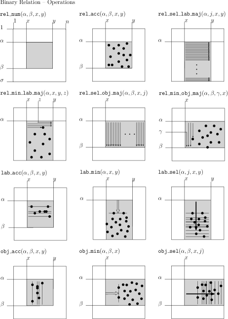
Figure 9: Some operations illustrated.

Appendix B Algorithms on BinRel-Str

We prove some of the complexities in Table 1. The others can be derived using Theorem 1.

Lemma 19.

BinRel-Str supports $\mathtt{rel\_num}(\alpha,\beta,x,y)$ in $O(\min((\beta-\alpha+1)r,(y-x+1)a\lg\beta))$ time.

Proof.

We can compute $\mathtt{rel\_num}(\alpha,\beta,x,y)$ in two ways:

• Using that $\mathtt{rel\_num}(\alpha,\beta,x,y)=\sum_{\alpha\leq\gamma\leq\beta}\mathtt{rel\_num}(\gamma,\gamma,x,y)$ and that $\mathtt{rel\_num}(\gamma,\gamma,x,y)=\mathtt{rank}_{\gamma}(S,\mathtt{map}(x-1)+1,\mathtt{map}(y))$, we achieve time $O((\beta-\alpha+1)r)$.

• Using that $\mathtt{rel\_num}(\alpha,\beta,x,y)=\sum_{x\leq z\leq y}\mathtt{rel\_num}(\alpha,\beta,z,z)$, we can compute the value for each $z$ by searching for the successor of $\alpha$ and the predecessor of $\beta$ in $S[\mathtt{map}(z-1)+1,\mathtt{map}(z)]$. As this range of $S$ is sorted we can find the predecessors and successors using exponential search, which requires in $O(\lg\beta)$ $\mathtt{access}$ operations. Thus the overall process takes time $O((y-x+1)a\lg\beta)$.

∎

Lemma 20.

BinRel-Str supports $\mathtt{lab\_num}(\alpha,\beta,x,y)$ in $O(\min((\beta-\alpha+1)r,(y-x+1)(\lg\alpha+\beta-\alpha)a))$ time.

Proof.

We can compute $\mathtt{lab\_num}(\alpha,\beta,x,y)$ in two ways:

• Using that $\mathtt{lab\_num}(\alpha,\beta,x,y)=\sum_{\alpha\leq\gamma\leq\beta}\mathtt{lab\_num}(\gamma,\gamma,x,y)$, and that $\mathtt{lab\_num}(\gamma,\gamma,x,y)=1$ iff $\mathtt{rel\_num}(\gamma,\gamma,x,y)>0$ and zero otherwise, we can achieve the same time as in the first alternative of Lemma 19.

• Using that $\mathtt{lab\_num}(\alpha,\beta,x,y)=|\cup_{x\leq z\leq y}\mathtt{lab\_acc}(\alpha,\beta,z,z)|$, we can collect the labels in $[\alpha,\beta]\times[z,z]$ for each $z$ and insert them into a dictionary. The labels related to a single $z$ can be found by using a similar method as the one in Lemma 19: use exponential search to find the first element $\geq\alpha$ in $z$’s area of $S$, and then scan the next symbols until surpassing $\beta$. We mark each label found in a bitmap of length $\beta-\alpha+1$, and then we report the number of ones in it.

∎

Lemma 21.

BinRel-Str supports $\mathtt{obj\_num}(\alpha,\beta,x,y)$ in $O(\min((y-x+1)a\lg\alpha,(\beta-\alpha+1)(r+(y-x+1)s)))$ time.

Proof.

We can compute $\mathtt{obj\_num}(\alpha,\beta,x,y)$ in two ways:

• Using that $\mathtt{obj\_num}(\alpha,\beta,x,y)=\sum_{x\leq z\leq y}\mathtt{obj\_num}(\alpha,\beta,z,z)$, and that $\mathtt{obj\_num}(\alpha,\beta,z,z)=1$ iff $\mathtt{rel\_num}(\alpha,\beta,z,z)>0$ and zero otherwise, we can proceed similarly as in the second alternative of Lemma 19, by exponentially searching for the first value $\geq\alpha$ in $z$’s area of $S$ and checking whether it is $\leq\beta$.

• Using that $\mathtt{obj\_num}(\alpha,\beta,x,y)=|\cup_{\alpha\leq\gamma\leq\beta}\mathtt{obj\_acc}(\gamma,\gamma,x,y)|$, we can collect the objects in $[\gamma,\gamma]\times[x,y]$ for each $\gamma$ and insert them into a dictionary, as in Lemma 20. The objects related to a single $\gamma$ can be found by using successive $\mathtt{select}_{\gamma}(S,j)$ operations on $S[\mathtt{map}(x-1)+1,\mathtt{map}(y)]$, starting with $j=\mathtt{rank}_{\gamma}(S,\mathtt{map}(x-1))+1$. The complexity considers the worst case where each such $\gamma$ appears $y-x+1$ times.

∎

Note that, when reducing to implement $\mathtt{obj\_rnk}$, the $\mathtt{rank}_{\gamma}(S,\cdot)$ operation is not necessary. For $\mathtt{obj\_rnk}1$ it is better to reduce from $\mathtt{rel\_num}$.

Lemma 22.

BinRel-Str supports $\mathtt{rel\_sel\_lab\_maj}(\alpha,j,x,y)$ in $O(\min((\sigma-\alpha)r+s,(y-x+1)(\sigma-\alpha+1)a))$ time.

Proof.

Again, we have two possible solutions:

• Set $c\leftarrow 0$. For each label $\gamma$ in $[\alpha,\sigma]$, compute $c^{\prime}\leftarrow c+\mathtt{rank}_{\gamma}(S,\mathtt{map}(x-1)+1,\mathtt{map}(y))$. If at some step it holds $c^{\prime}\geq j$, the answer is $(\gamma,\mathtt{unmap}(\mathtt{select}_{\gamma}(S,j-c+\mathtt{rank}_{\gamma}(S,\mathtt{map}(x-1))))$. Otherwise, update $c\leftarrow c^{\prime}$. The overall process takes $O((\sigma-\alpha+1)r+s)$ time.

• Similarly, but first accumulating all the occurrences of all the labels $\gamma$ and then finding $j$ using the accumulators. We simply traverse the area $S[\mathtt{map}(z-1)+1,\mathtt{map}(z)]$ backwards, for each $z\in[x,y]$, accessing each label $S[k]$ and incrementing the corresponding counter. The process takes $O((y-x+1)(\sigma-\alpha+1)a)$ time.

∎

From this operation we can obtain complexities for $\mathtt{rel\_min\_lab\_maj}$, $\mathtt{lab\_min}$, $\mathtt{lab\_min1}$, $\mathtt{lab\_acc}$, and $\mathtt{lab\_acc1}$. Some of the results we give are better than those obtained by a blind reduction; we leave to the reader to check these improvements. We also note that an obvious variant of this algorithm is our best solution to compute $\mathtt{lab\_sel}$, within the same time.

Lemma 23.

BinRel-Str supports $\mathtt{rel\_sel\_obj\_maj}(\alpha,\beta,x,j)$ in $O(\min((n-x+1)a\lg\beta,(\beta-\alpha+1)((n-x+1)s+r)))$ time.

Proof.

Once again, we have two possible solutions:

• Set $c\leftarrow 0$. For each object $z$ in $[x,n]$, use exponential search on $z$’s area of $S$ to find the range $S[a,b]$ corresponding to $[\alpha,\beta]$, and set $c^{\prime}\leftarrow c+b-a+1$. If at some step it holds $c^{\prime}\geq j$, the answer is $(S[j-c+a-1],z)$. Otherwise, update $c\leftarrow c^{\prime}$. The overall process takes $O((n-x+1)a\lg\beta)$ time.

• Similarly, but first accumulating all the occurrences of all the objects $z$ and then finding $j$ using the accumulators. We traverse the area $S[\mathtt{map}(x-1)+1,\mathtt{map}(y)]$ for each label $\gamma$ in $[\alpha,\beta]$, using successive $\mathtt{select}_{\gamma}(S,j^{\prime})$ queries, starting at $j^{\prime}=\mathtt{rank}_{\gamma}(S,\mathtt{map}(x-1))+1$. The process takes $O((\beta-\alpha+1)((n-x+1)s+r))$ time.

∎

From this operation we can obtain complexities for $\mathtt{rel\_min\_obj\_maj}$, $\mathtt{rel\_acc}$, $\mathtt{obj\_min}$, $\mathtt{obj\_min1}$, $\mathtt{obj\_acc}$, and $\mathtt{obj\_acc1}$. Once again, some of the results we give are better than a blind reduction and we leave the reader to verify those. Finally, an obvious variant of this algorithm is our best solution to compute $\mathtt{obj\_sel}$.

A final easy exercise for the reader is to show that $\mathtt{lab\_sel1}(\alpha,j,x)$ can be solved in time $O(a\lg\alpha)$, and that $\mathtt{obj\_sel1}(\alpha,x,j)$ is solved in time $O(r+s)$.

References

- [1] D. Arroyuelo, G. Navarro, and K. Sadakane. Stronger Lempel-Ziv based compressed text indexing. Algorithmica, 62(1):54–101, 2012.
- [2] J. Barbay, L. Aleardi, M. He, and J. Munro. Succinct representation of labeled graphs. Algorithmica, 62(1-2):224–257, 2012.
- [3] J. Barbay, F. Claude, and G. Navarro. Compact rich-functional binary relation representations. In Proc. 9th Latin American Symposium on Theoretical Informatics (LATIN), LNCS 6034, pages 170–183, 2010.
- [4] J. Barbay, T. Gagie, G. Navarro, and Y. Nekrich. Alphabet partitioning for compressed rank/select and applications. In Proc. 21st Annual International Symposium on Algorithms and Computation (ISAAC), LNCS 6507, pages 315–326. Springer, 2010. Part II.
- [5] J. Barbay, A. Golynski, I. Munro, and S. S. Rao. Adaptive searching in succinctly encoded binary relations and tree-structured documents. Theoretical Computer Science, 387(3):284–297, 2007.
- [6] J. Barbay, M. He, I. Munro, and S. S. Rao. Succinct indexes for strings, binary relations and multi-labeled trees. In Proc. 18th Symposium on Discrete Algorithms (SODA), pages 680–689, 2007.
- [7] J. Barbay, A. López-Ortiz, T. Lu, and A. Salinger. An experimental investigation of set intersection algorithms for text searching. ACM Journal of Experimental Algorithmics, 14, 2009.
- [8] J. Barbay and G. Navarro. Compressed representations of permutations, and applications. In Proc. 26th International Symposium on Theoretical Aspects of Computer Science (STACS), pages 111–122, 2009.
- [9] P. Boldi and S. Vigna. The WebGraph framework I: compression techniques. In Proc. 13th World Wide Web Conference (WWW), pages 595–602, 2004.
- [10] P. Bose, M. He, A. Maheshwari, and P. Morin. Succinct orthogonal range search structures on a grid with applications to text indexing. In Proc. 20th Symposium on Algorithms and Data Structures (WADS), pages 98–109, 2009.
- [11] N. Brisaboa, S. Ladra, and G. Navarro. K2-trees for compact web graph representation. In Proc. 16th International Symposium on String Processing and Information Retrieval (SPIRE), LNCS 5721, pages 18–30, 2009.
- [12] Y.-F. Chien, W.-K. Hon, R. Shah, and J. Vitter. Geometric Burrows-Wheeler transform: Linking range searching and text indexing. In Proc. 18th Data Compression Conference (DCC), pages 252–261, 2008.
- [13] D. Clark. Compact Pat Trees. PhD thesis, Univ. of Waterloo, Canada, 1996.
- [14] F. Claude and G. Navarro. Extended compact Web graph representations. In T. Elomaa, H. Mannila, and P. Orponen, editors, Algorithms and Applications (Ukkonen Festschrift), LNCS 6060, pages 77–91. Springer, 2010.
- [15] F. Claude and G. Navarro. Fast and compact Web graph representations. ACM Transactions on the Web, 4(4):article 16, 2010.
- [16] F. Claude and G. Navarro. Self-indexed grammar-based compression. Fundamenta Informaticae, 111(3):313–337, 2010.
- [17] A. Farzan, T. Gagie, and G. Navarro. Entropy-bounded representation of point grids. In Proc. 21st Annual International Symposium on Algorithms and Computation (ISAAC), LNCS 6507, pages 327–338, 2010. Part II.
- [18] P. Ferragina, G. Manzini, V. Mäkinen, and G. Navarro. Compressed representations of sequences and full-text indexes. ACM Transactions on Algorithms, 3(2):article 20, 2007.
- [19] J. Fischer. Optimal succinctness for range minimum queries. In Proc. 9th Symposium on Latin American Theoretical Informatics (LATIN), LNCS 6034, pages 158–169, 2010.
- [20] T. Gagie, G. Navarro, and S. Puglisi. New algorithms on wavelet trees and applications to information retrieval. Theoretical Computer Science, 2011. . To appear. http://arxiv.org/abs/1011.4532.
- [21] A. Golynski. Optimal lower bounds for rank and select indexes. Theoretical Computer Science, 387(3):348–359, 2007.
- [22] A. Golynski, I. Munro, and S. Rao. Rank/select operations on large alphabets: a tool for text indexing. In Proc. 17th Annual Symposium on Discrete Algorithms (SODA), pages 368–373, 2006.
- [23] A. Golynski, R. Raman, and S. Rao. On the redundancy of succinct data structures. In Proc. 11th Scandinavian Workshop on Algorithm Theory (SWAT), LNCS 5124, pages 148–159, 2008.
- [24] R. Grossi, A. Gupta, and J. Vitter. High-order entropy-compressed text indexes. In Proc. 14th Annual Symposium on Discrete Algorithms (SODA), pages 841–850, 2003.
- [25] J. Kärkkäinen. Repetition-Based Text Indexing. PhD thesis, U. Helsinki, Finland, 1999.
- [26] S. Kreft and G. Navarro. Self-indexing based on LZ77. In Proc. 22nd Annual Symposium on Combinatorial Pattern Matching (CPM), LNCS 6661, pages 41–54, 2011.
- [27] V. Mäkinen and G. Navarro. Rank and select revisited and extended. Theoretical Computer Science, 387(3):332–347, 2007.
- [28] V. Mäkinen and G. Navarro. Dynamic entropy-compressed sequences and full-text indexes. ACM Transactions on Algorithms, 4(3):article 32, 2008.
- [29] S. Muthukrishnan. Efficient algorithms for document retrieval problems. In Proc 13th Annual Symposium on Discrete Algorithms (SODA), pages 657–666, 2002.
- [30] G. Navarro and L. Russo. Space-efficient data analysis queries on grids. CoRR, 1106.4649, 2011. http://arxiv.org/abs/1106.4649.
- [31] M. Pătraşcu. Lower bounds for 2-dimensional range counting. In Proc. 39th Annual ACM Symposium on Theory of Computing (STOC), pages 40–46, 2007.
- [32] M. Pătraşcu. Succincter. In Proc. 49th Annual Symposium on Foundations of Computer Science (FOCS), pages 305–313, 2008.
- [33] R. Raman, V. Raman, and S. S. Rao. Succinct indexable dictionaries with applications to encoding -ary trees and multisets. In Proc. 13th Annual Symposium on Discrete Algorithms (SODA), pages 233–242, 2002.
- [34] I. Witten, A. Moffat, and T. Bell. Managing Gigabytes. Morgan Kaufmann Publishers, 2nd edition, 1999.