Covariance Eigenvector Sparsity for
Compression and Denoising

Ioannis D. Schizas and Georgios B. Giannakis
Abstract

Sparsity in the eigenvectors of signal covariance matrices is exploited in this paper for compression and denoising. Dimensionality reduction (DR) and quantization modules present in many practical compression schemes such as transform codecs, are designed to capitalize on this form of sparsity and achieve improved reconstruction performance compared to existing sparsity-agnostic codecs. Using training data that may be noisy a novel sparsity-aware linear DR scheme is developed to fully exploit sparsity in the covariance eigenvectors and form noise-resilient estimates of the principal covariance eigenbasis. Sparsity is effected via norm-one regularization, and the associated minimization problems are solved using computationally efficient coordinate descent iterations. The resulting eigenspace estimator is shown capable of identifying a subset of the unknown support of the eigenspace basis vectors even when the observation noise covariance matrix is unknown, as long as the noise power is sufficiently low. It is proved that the sparsity-aware estimator is asymptotically normal, and the probability to correctly identify the signal subspace basis support approaches one, as the number of training data grows large. Simulations using synthetic data and images, corroborate that the proposed algorithms achieve improved reconstruction quality relative to alternatives.

Index Terms:
PCA, data compression, subspace estimation, denoising, quantization.
000${\dagger}$ Manuscript received October 7, 2010; accepted January 7, 2012. First published XXXXXX XX, 20XX; current version published XXXXXX XX, 20XX. The associate editor coordinating the review of this manuscript and approving it for publication was Dr. Maja Bystrom. Work in this paper was supported by the NSF Grant CCF-1016605. Part of the paper was presented in the 3rd Intl. Workshop on Comp. Advances in Multi-Sensor Adap. Proc., Aruba, Dutch Antilles, Dec. 2009.000$*$ Ioannis Schizas is with the Dept. of Electrical Engineering, University of Texas at Arlington, 416 Yates Street, Arlington, TX 76011. Tel/fax: (817) 272-3467/272-2253. Georgios Giannakis is with the Dept. of Electrica and Computer Engineering, University of Minnesota, 200 Union Street SE, Minneapolis, MN 55455; Emails: {schizas@uta.edu,georgios@umn.edu}.

I Introduction

Data compression has well-appreciated impact in audio, image and video processing since the increasing data rates cannot be matched by the computational and storage capabilities of existing processors. The cornerstone modules of compression are those performing dimensionality reduction (DR) and quantization, as in e.g., transform codecs [16]. DR projects the data onto a space of lower dimension while minimizing an appropriate figure of merit quantifying information loss. Quantization amounts to digitizing the analog-amplitude DR data. Typically, DR relies on training vectors to find parsimonious data representations with reduced redundancy without inducing, e.g., mean-square error (MSE) distortion in the reconstruction process. One such property that promotes parsimony is sparsity.

Sparsity is an attribute characterizing many natural and man-made signals [2], and has been successfully exploited in statistical inference tasks using the least-absolute shrinkage and selection operator (Lasso) [29, 35]. In parallel, recent results in compressive sampling rely on sparsity to solve under-determined systems of linear equations, as well as sample continuous signals at sub-Nyquist rates [7]. These tasks take advantage of sparsity present in deterministic signal descriptors. But what if sparsity is present in statistical descriptors such as the signal covariance matrix? The latter is instrumental in compression when the distortion metric is MSE. In bio-informatics and imaging applications the data input to the DR module have covariance matrices whose eigenvectors admit a sparse representation over a certain domain, such as the wavelet domain [18].

The ‘workhorse’ for DR is principal component analysis (PCA) [5, 19], which relies on the covariance matrix to project the data on the subspace spanned by its principal eigenvectors. So far, sparsity has been exploited for interpreting each principal component, but not for reconstructing reduced-dimension signal renditions. Specifically, the standard PCA criterion has been regularized with an $\ell_{1}$-norm penalty term to induce sparsity as in the Lasso, and perform variable selection of the data entries that significantly contribute to each principal component [20]. However, the nonconvex formulation of [20] does not lend itself to efficient optimization. The sparse PCA formulation in [36] leads to a cost minimized using the block coordinate descent optimization method [3]; see also [23] which includes a weighted $\ell_{1}$-norm sparsity-imposing penalty. PCA with cardinality constraints on the number of nonzero elements per principal eigenvector has also been considered using relaxation techniques [9, 8]. Alternative approaches augment the standard singular value decomposition (SVD) cost, or the maximum likelihood criterion with $\ell_{1}$ (or $\ell_{0}$) penalties to effect sparsity in the principal eigenvectors [33, 27, 31, 32, 18]. Sparsity has also been exploited to render PCA robust to outliers [6], as well as to reduce complexity at the encoder [12]. In all the aforementioned schemes sparsity is not exploited for reconstructing signals that have been compressed by DR and quantization.

When dealing with noisy data, pertinent reconstruction techniques have been developed to perform joint denoising and signal reconstruction [26, 28, 25]. However, existing approaches rely on the noise second-order statistics being available. Here, the a priori knowledge that the signal covariance eigenvectors are sparse is exploited, and joint denoising-reconstruction schemes are introduced without requiring availability of the noise covariance.

The standard PCA cost is augmented with pertinent $\ell_{1}-$ and $\ell_{2}-$norm regularization terms, that fully exploit the sparsity present in the covariance eigenvectors when performing not only feature extraction (as in [20, 36, 9, 33]) but also reconstruction. The resulting bilinear cost is minimized via coordinate descent which leads to an efficient sparse (S-) PCA algorithm for DR and reconstruction.Its large-sample performance is analyzed in the presence of observation noise. If the ensemble covariance matrix of the noisy training data is known, then the sparsity-aware estimates do better in terms of identifying the support of the principal basis vectors when compared to the standard sparsity-agnostic PCA. As the number of training data used to design the DR module grows large, the novel sparsity-aware signal covariance eigenspace estimators: i) are asymptotically normal; and ii) identify the true principal eigenvectors’ support (indices of nonzero elements) with probability one. The last two properties, known as ‘oracle’ properties [35], combined with the noise-resilience enable the novel S-PCA to attain an improved trade-off between reconstruction performance and reduced-dimensionality-a performance advantage also corroborated via numerical examples. The proposed sparsity-aware DR scheme is finally combined with a vector quantizer (VQ) to obtain a sparsity-aware transform coder (SATC), which improves reconstruction performance when compared to standard TC schemes that rely on the discrete cosine transform (DCT) or PCA transform. The merits of SATC are also demonstrated in the compression and reconstruction/denoising of noisy images that have been extracted from [1].

The rest of the paper is organized as follows. After stating the problem setting in Sec. II, the proposed sparsity-aware PCA formulation is introduced in Sec. III-A. Coordinate descent is employed in Sec. III-B to minimize the associated bilinear cost, while a computationally simpler element-wise algorithm is derived in Sec. III-C. A cross-validation scheme is outlined in Sec. III-D for selecting the sparsity-controlling coefficients that weigh the $\ell_{1}$-norm based regularization terms. Asymptotic properties are derived both in the noiseless and noisy cases, establishing the potential of the novel estimators to recover the underlying signal covariance principal eigenvectors (Secs. IV-A, IV-B). S-PCA is combined with vector quantization in Sec. V. Synthetic numerical examples (Sec. VI-A) illustrate the performance advantage of SATC, while tests using real noisy images corroborate the potential of SATC in practical settings (Sec. VI-B).

II Preliminaries and Problem Formulation

Consider a collection of $n$ training data vectors $\{{\mathbf{x}}_{t}={\mathbf{s}}_{t}+{\mathbf{w}}_{t}\}_{t=1}^{n}$, each containing the signal of interest ${\mathbf{s}}_{t}\in\mathbb{R}^{p\times 1}$, in additive zero-mean possibly colored noise ${\mathbf{w}}_{t}$, assumed independent of ${\mathbf{s}}_{t}$. It is also assumed that ${\mathbf{s}}_{t}$ lies in a linear subspace of reduced dimension, say $r\leq p$, spanned by an unknown orthogonal basis $\{{\mathbf{u}}_{s,\rho}\}_{\rho=1}^{r}$. Many images and audio signals lie on such a low-dimensional subspace. Accordingly, ${\mathbf{s}}_{t}$ for such signals can be expressed as

$${\mathbf{s}}_{t}={\mbox{\boldmath$\mu$}}_{s}+\sum_{\rho=1}^{r}\pi_{t,\rho}{\mathbf{u}}_{s,\rho},\;\;\;t=1,\ldots,n$$ (1)

where ${\mbox{\boldmath$\mu$}}_{s}$ denotes the mean of ${\mathbf{s}}_{t}$, and $\pi_{t,\rho}$ are zero-mean independent projection coefficients.

The covariance matrix of the noisy ${\mathbf{x}}_{t}$ is given by ${\mbox{\boldmath$\Sigma$}}_{x}={\mbox{\boldmath$\Sigma$}}_{s}+{\mbox{\boldmath$\Sigma$}}_{w}$, where ${\mbox{\boldmath$\Sigma$}}_{s}$ (${\mbox{\boldmath$\Sigma$}}_{w}$) denotes the signal (noise) covariance matrix. Consider the eigen-decomposition ${\mbox{\boldmath$\Sigma$}}_{w}={\mathbf{U}}_{w}{\mathbf{D}}_{w}{\mathbf{U}}_{w}^{T}$, where ${\mathbf{U}}_{w}$ denotes the eigen-matrix containing the eigenspace basis, and ${\mathbf{D}}_{w}:=\textrm{diag}(d_{w,1},\ldots d_{w,p})$ the corresponding eigenvalues (T denotes matrix transposition). Likewise, for the signal covariance matrix let ${\mbox{\boldmath$\Sigma$}}_{s}={\mathbf{U}}_{s}{\mathbf{D}}_{s}{\mathbf{U}}_{s}^{T}={\mathbf{U}}_{s,r}{\mathbf{D}}_{s,r}{\mathbf{U}}_{s,r}^{T}$ where ${\mathbf{U}}_{s,r}:=[{\mathbf{u}}_{s,1}\ldots{\mathbf{u}}_{s,r}]$ and ${\mathbf{D}}_{s,r}:=\textrm{diag}(d_{s,1},\ldots,d_{s,r})$ contain the $r$ dominant eigenvectors and eigenvalues of ${\mbox{\boldmath$\Sigma$}}_{s}$, respectively; while $d_{s,\rho}:={E}[\pi_{\rho,t}^{2}]$. Further, let ${\mathbf{U}}_{s,p-r}\in\mathbb{R}^{p\times(p-r)}$ denote the matrix formed by the subspace of dimensionality $p-r$, which is perpendicular to the signal subspace ${\mathbf{U}}_{s,r}$. In the following, ${\mbox{\boldmath$\mu$}}_{s}$ is assumed known and subtracted from ${\mathbf{s}}_{t}$; thus, without loss of generality (wlog) ${\mathbf{x}}_{t}$ and ${\mathbf{s}}_{t}$ are assumed zero-mean. Matrices ${\mbox{\boldmath$\Sigma$}}_{s}$ and ${\mbox{\boldmath$\Sigma$}}_{w}$ are not available, which is the case in several applications. Moreover, the following is assumed about sample covariances.
(a1) The signal of interest ${\mathbf{s}}_{t}$ and observation noise ${\mathbf{w}}_{t}$ are independent across time $t$ and identically distributed. Thus, by the strong law of large numbers the sample covariance matrix estimate $\hat{{\mbox{\boldmath$\Sigma$}}}_{x,n}:=n^{-1}\sum_{t=1}^{n}{\mathbf{x}}_{t}{\mathbf{x}}_{t}^{T}$ converges almost surely, as $n\rightarrow\infty$, to the ensemble covariance matrix ${\mbox{\boldmath$\Sigma$}}_{x}$.

Consider next a unitary transformation matrix ${\mathbf{F}}\in\mathbb{R}^{p\times p}$ to form the transformed data

$$\check{{\mathbf{x}}}_{t}:={\mathbf{F}}{\mathbf{x}}_{t}=\sum_{\rho=1}^{r}\pi_{t,\rho}{\mathbf{F}}{\mathbf{u}}_{s,\rho}+{\mathbf{F}}{\mathbf{w}}_{t}.$$ (2)

Such a mapping could represent the wavelet, Fourier, or, the discrete cosine transform (DCT). The case of interest here is when ${\mathbf{F}}$ is such that the transformed eigenvectors $\check{{\mathbf{u}}}_{s,\rho}:={\mathbf{F}}{\mathbf{u}}_{s,\rho}$ of ${\mbox{\boldmath$\Sigma$}}_{\check{s}}$, where $\check{{\mathbf{s}}}:={\mathbf{F}}{\mathbf{s}}$, have many entries equal to zero, i.e., ${\mbox{\boldmath$\Sigma$}}_{\check{s}}$ has sparse eigenvectors. One natural question is whether eigenvectors of a covariance matrix admit a sparse representation over e.g., the DCT domain. Often in bio-informatics and imaging applications the data input to the DR module have covariance matrix with sparse eigenvectors [18]. The same attribute is also present in other classes of signals. Consider for instance signal vectors comprising uncorrelated groups of entries, with each group containing correlated entries – a case where the covariance matrix is block diagonal. In addition to block diagonal covariance matrices, the class also includes row- and/or column-permuted versions of block diagonal covariance matrices.

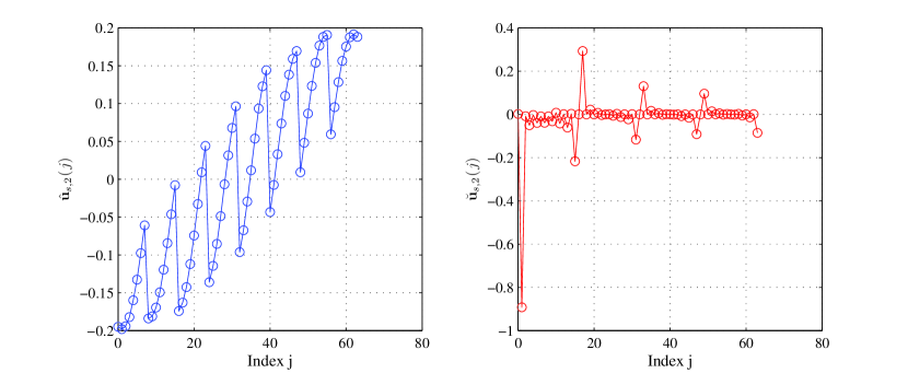
An example is provided next to demonstrate that ${\mbox{\boldmath$\Sigma$}}_{\check{s}}$ can have sparse eigenvectors. A high-resolution image taken from [1] displaying part of the Martian terrain, was split into $112$ smaller non-overlapping images of size $180\times 256$. Each of these images was further split into $8\times 8$ blocks. Vectors $\{{{\mathbf{s}}}_{t}\}_{t=1}^{112}$ correspond to a block (here the $10$th after lexicographically scanning each of the $112$ sub-images) comprising entries with the same row and column indices in all $112$ different sub-images. An estimate of the underlying covariance matrix of the vectorized blocks is formed using sample averaging, to obtain $\hat{{\mbox{\boldmath$\Sigma$}}}_{s}:=(112)^{-1}\sum_{t=1}^{112}{\mathbf{s}}_{t}{\mathbf{s}}_{t}^{T}$. The $\textrm{rank}(\hat{{\mbox{\boldmath$\Sigma$}}}_{s})=15$ indicates that the $64\times 1$ vectorized image blocks lie approximately in a linear subspace of $\mathbb{R}^{64\times 1}$ having dimension $r=15$. This subspace is spanned by the $15$ principal eigenvectors of $\hat{{\mbox{\boldmath$\Sigma$}}}_{s}$ and forms the signal subspace. To explore whether the principal eigenvectors of ${\mbox{\boldmath$\Sigma$}}_{s}$ have a hidden sparsity structure that could be exploited during DR Fig. 1 (left) depicts the value for each of the entries of the second principal eigenvector of $\hat{{\mbox{\boldmath$\Sigma$}}}_{s}$, namely $\hat{{\mathbf{u}}}_{s,2}$, versus the index number of each entry. Note that the entries of $\hat{{\mathbf{u}}}_{s,2}$ exhibit a sinusoidal behavior; thus, if DCT is applied to $\hat{{\mathbf{u}}}_{s,2}$ the resulting vector $\check{{\mathbf{u}}}_{s,2}=\mathbf{F}\hat{{\mathbf{u}}}_{s,2}$ has only a few DCT coefficients with large magnitude. Indeed, Fig. 1 (right) corroborates that $\hat{{\mathbf{u}}}_{x,2}$ is sparse over the DCT domain. In fact, all $15$ principal eigenvectors of $\hat{{\mbox{\boldmath$\Sigma$}}}_{s}$ admit a sparse representation over the DCT domain as the one displayed in Fig. 1 (right). Thus, the sample covariance matrix of the transformed vectorized blocks $\check{{\mathbf{s}}}_{t}={\mathbf{F}}{\mathbf{s}}_{t}$ has $15$ principal eigenvectors that exhibit high degree of sparsity. Such a sparse structure is to be expected since images generated from [1] exhibit localized features (hilly terrain), which further result in sparse signal basis vectors in the DCT domain[18]. For simplicity, the original notation ${\mathbf{x}}_{t}$, ${\mathbf{s}}_{t}$ and ${\mathbf{w}}_{t}$ will henceforth refer to the DCT transformed training data, signal of interest, and observation noise, respectively.

Aiming to compress data vector ${\mathbf{x}}$, linear DR is performed at the encoder by left-multiplying $\mathbf{x}$ with a fat matrix $\mathbf{C}\in\mathbf{R}^{q\times p}$, where $q\leq r\leq p$. The reduced dimension $q$ may be chosen smaller than the signal subspace dimension $r$, when resources are limited. Vector $\mathbf{C}\mathbf{x}$ is received at the decoder where it is left-multiplied by a tall $p\times q$ matrix ${\mathbf{B}}$ to reconstruct ${\mathbf{s}}$ as $\hat{\mathbf{s}}:=\mathbf{B}\mathbf{Cx}$. Matrices ${{\mathbf{B}}}$ and ${{\mathbf{C}}}$ should be selected such that $\hat{\mathbf{s}}=\mathbf{B}\mathbf{Cx}$ forms a ‘good’ estimate of ${\mathbf{s}}$. One pair of matrices $\mathbf{B}_{o},\mathbf{C}_{o}$, minimizing the reconstruction MSE

$$({\mathbf{B}}_{o},{\mathbf{C}}_{o})\in\arg\min_{{\mathbf{B}},{\mathbf{C}}}E[\|\mathbf{s}-\mathbf{BC}\mathbf{x}\|^{2}]$$ (3)

are given as ${\mathbf{C}}_{o}={\mathbf{U}}_{sx,q}^{T}{\mbox{\boldmath$\Sigma$}}_{sx}{\mbox{\boldmath$\Sigma$}}_{x}^{-1},\;\;{\mathbf{B}}_{o}={\mathbf{U}}_{sx,q}$, where ${\mathbf{U}}_{sx,q}$ are the $q$ principal eigenvectors of ${\mbox{\boldmath$\Sigma$}}_{sx}{\mbox{\boldmath$\Sigma$}}_{x}^{-1}{\mbox{\boldmath$\Sigma$}}_{sx}^{T}$, while the $\in$ notation emphasizes that (3) does not have a unique optimal solution (e.g., see [5, Ch. 10]). In the absence of observation noise, (${\mathbf{x}}_{t}={\mathbf{s}}_{t}$), (3) corresponds to the standard PCA, where a possible choice for ${\mathbf{B}}_{o},{\mathbf{C}}_{o}$ is $\mathbf{B}_{o}=\mathbf{U}_{s,q}$ and $\mathbf{C}_{o}=\mathbf{U}_{s,q}^{T}$[5, Ch. 9]. Since the ensemble covariance matrices are not available; ${\mathbf{C}}_{o}$ and ${\mathbf{B}}_{o}$ cannot be found. The practical approach is to replace the cost in (3) with its sample-averaged version $n^{-1}\|\mathbf{S}-\mathbf{BC}\mathbf{X}\|_{F}^{2}$, where ${\mathbf{S}}:=[{\mathbf{s}}_{1}\ldots{\mathbf{s}}_{n}]$ and ${\mathbf{X}}:=[{\mathbf{x}}_{1}\ldots{\mathbf{x}}_{n}]$. This would require training samples for both ${\mathbf{x}}$, and the signal of interest ${\mathbf{s}}$[5, Ch. 10]. This is impossible in the noisy setting considered here. The reduced dimension $q\leq p$ can be selected depending on the desired reduction viz reconstruction error afforded.

In the noiseless case, the optimal DR and reconstruction matrices are formed using the signal eigenvectors, that is ${\mathbf{C}}_{o}={\mathbf{B}}_{o}^{T}={\mathbf{U}}_{s,q}^{T}$. But even in the noisy case, the signal subspace ${\mathbf{U}}_{s,q}$ is useful for joint DR and denoising [26, 25, 28, 34]. Indeed, if ${\mathbf{C}}={\mathbf{B}}^{T}={\mathbf{U}}_{s,q}^{T}$, then it is easy to see that $J_{\textrm{rec}}({\mathbf{B}},{\mathbf{C}}):=E[\|{\mathbf{s}}-{\mathbf{B}}{\mathbf{C}}{\mathbf{x}}\|_{2}^{2}]=\textrm{tr}({\mbox{\boldmath$\Sigma$}}_{w})-\textrm{tr}({{\mathbf{U}}}_{s,p-q}^{T}{\mbox{\boldmath$\Sigma$}}_{w}{{\mathbf{U}}}_{s,p-q})<\textrm{tr}({\mbox{\boldmath$\Sigma$}}_{w})$ when $q=r<p$. Thus, projection of ${\mathbf{x}}_{t}$ onto the signal subspace not only achieves DR but also reduces noise effects. The question of course is how to form an estimate for ${\mathbf{U}}_{s,q}$ when ${\mbox{\boldmath$\Sigma$}}_{x}$ and ${\mbox{\boldmath$\Sigma$}}_{w}$ are unknown. Existing signal subspace estimators assume either that i) the noise is white, namely ${\mbox{\boldmath$\Sigma$}}_{w}=\sigma_{w}^{2}{\mathbf{I}}_{p}$ for which ${\mathbf{U}}_{x}={\mathbf{U}}_{s}$ (${\mathbf{I}}_{p}$ denotes the $p\times p$ identity matrix); or, ii) the ${\mbox{\boldmath$\Sigma$}}_{w}$ is known or can be estimated via sample-averaging [26, 25, 28, 34]. In the setting here these assumptions are not needed.

Based on training data $\{{\mathbf{x}}_{t}\}_{t=1}^{n}$, the major goal is to exploit the sparsity present in the eigenvectors of $\mathbf{{\mbox{\boldmath$\Sigma$}}}_{s}$ in order to derive estimates $\hat{{\mathbf{B}}},\hat{{\mathbf{C}}}$ for the signal subspace ${\mathbf{U}}_{s,q}$, thereby achieving a better trade-off between the reduced-dimension $q$ and the MSE cost $J_{\textrm{rec}}({\mathbf{B}},{\mathbf{C}})$ than existing alternatives [20, 36, 9, 33]. Towards this end, a novel sparsity-aware signal subspace estimator is developed in the next section. Since the majority of data processing and communication systems are digital, this sparsity-exploiting DR step will be followed by a sparsity-cognizant VQ step in order to develop a sparsity-aware transform coding (SATC) scheme for recovering ${\mathbf{s}}_{t}$ based on quantized DR data.

III Sparse Principal Component Analysis

Recall that the standard PCA determines DR and reconstruction matrices $\hat{{\mathbf{C}}}_{o}$ and $\hat{{\mathbf{B}}}_{o}$ by minimizing the sample-based cost $\hat{J}_{\textrm{rec}}({\mathbf{B}},{\mathbf{C}}):=n^{-1}\|{\mathbf{X}}-{\mathbf{B}}{\mathbf{C}}{\mathbf{X}}\|_{F}^{2}$. One possible minimizer for the latter is $\hat{{\mathbf{B}}}_{o}=\hat{{\mathbf{C}}}_{o}^{T}=\hat{{\mathbf{U}}}_{x,q}$, where $\hat{{\mathbf{U}}}_{x,q}$ comprises the $q$ dominant eigenvectors of $\hat{{\mbox{\boldmath$\Sigma$}}}_{x}$. In the noiseless case it holds that $\hat{{\mbox{\boldmath$\Sigma$}}}_{x}=\hat{{\mbox{\boldmath$\Sigma$}}}_{s}$, from which it follows that $\hat{{\mathbf{U}}}_{x,q}=\hat{{\mathbf{U}}}_{s,q}$. However, the $q$-dominant eigenvectors of ${\mbox{\boldmath$\Sigma$}}_{x}$ do not coincide with $\hat{{\mathbf{U}}}_{s,q}$ when the additive noise is colored (${\mbox{\boldmath$\Sigma$}}_{w}\neq\sigma_{w}^{2}{\mathbf{I}}_{p}$). In this case, standard PCA is not expected to estimate reliably the signal subspace.

III-A An $\ell_{1}$-regularized formulation

Here the standard PCA formulation is enhanced by exploiting the sparsity present in ${\mathbf{U}}_{s,r}$. Prompted by Lasso-based sparse regression and PCA approaches [29, 20, 36, 9, 33], the quadratic cost of standard PCA is regularized with the $\ell_{1}$-norm of the unknowns to effect sparsity. Specifically, ${\mathbf{B}}_{o}={\mathbf{C}}_{o}^{T}={\mathbf{U}}_{s,q}$ could be estimated as

$$\arg\min_{{\mathbf{B}},{\mathbf{C}}}n^{-1}\|{\mathbf{X}}-{\mathbf{B}}{\mathbf{C}}{\mathbf{X}}\|_{F}^{2}+\sum_{\rho=1}^{q}\sum_{j=1}^{p}\lambda_{\rho}(|\mathbf{C}(\rho,j)|+|\mathbf{B}(j,\rho)|),\;\textrm{s. to }{\mathbf{B}}={\mathbf{C}}^{T}$$ (4)

which promotes sparsity in ${\mathbf{U}}_{s,r}$. However, the constraint ${\mathbf{B}}={\mathbf{C}}^{T}$ leads to a nonconvex problem that cannot be solved efficiently. This motivates the following ‘relaxed’ version of (4), where the wanted matrices are obtained as

$\displaystyle(\hat{{\mathbf{B}}},\hat{{\mathbf{C}}})$ $\displaystyle\in\arg\min_{{\mathbf{B}},{\mathbf{C}}}n^{-1}\|{\mathbf{X}}-{\mathbf{B}}{\mathbf{C}}{\mathbf{X}}\|_{F}^{2}+\sum_{\rho=1}^{q}\sum_{j=1}^{p}\lambda_{\rho}(|\mathbf{C}(\rho,j)|+|\mathbf{B}(j,\rho)|)+\mu\|{\mathbf{B}}-{\mathbf{C}}^{T}\|_{F}^{2}$ (5)

using efficient coordinate descent solvers. Note that $q\leq r$, since the dimensionality of the signal subspace may not be known. Moreover, $\{\lambda_{\rho}\}_{\rho=1}^{q}$ are nonnegative constants controlling the sparsity of $\mathbf{B}$ and $\mathbf{C}$. Indeed, the larger $\lambda_{\rho}$’s are chosen, the closer the entries of ${\mathbf{B}}$ and ${\mathbf{C}}$ are driven to the origin. Taking into account that the ‘clairvoyant’ compression and reconstruction matrices satisfy ${\mathbf{B}}_{o}={\mathbf{C}}_{o}^{T}={\mathbf{U}}_{s,q}$, the term $\mu\|{\mathbf{B}}-{\mathbf{C}}^{T}\|_{F}^{2}$ ensures that $\hat{{\mathbf{B}}}$ and $\hat{{\mathbf{C}}}^{T}$ stay close. Although ${\mathbf{B}}_{o}$ and ${\mathbf{C}}_{o}$ are orthonormal, ${\mathbf{B}}$ and ${\mathbf{C}}$ are not constrained to be orthonormal in (5) because orthonormality constraints of the form ${\mathbf{B}}^{T}{\mathbf{B}}=\mathbf{I}$ and ${\mathbf{C}}{\mathbf{C}}^{T}=\mathbf{I}$ are nonconvex. With such constraints present, efficient coordinate descent algorithms converging to a stationary point cannot be guaranteed.

Remark 1: The minimization problem in (5) resembles the sparse PCA formulation proposed in [36]. However, the approach followed in [36] imposes sparsity only on $\mathbf{C}$, while it forces matrix $\mathbf{B}$ to be orthonormal. The latter constraint mitigates scaling issues (otherwise $\mathbf{C}$ could be made arbitrarily small by counter-scaling $\mathbf{B}$), but is otherwise not necessarily well-motivated. Without effecting sparsity in ${\mathbf{B}}$, the formulation in [36] does not fully exploit the sparsity present in the eigenvectors of ${\mbox{\boldmath$\Sigma$}}_{s}$, which further results in sparse clairvoyant matrices $\mathbf{C}_{o}$ and $\mathbf{B}_{o}$ in the absence of noise. Notwithstanding, (5) combines the reconstruction error $n^{-1}\|\mathbf{X}-\mathbf{BCX}\|_{F}^{2}$ with regularization terms that impose sparsity to both $\mathbf{B}$ and $\mathbf{C}$. Even though the $\ell_{1}$-norm of ${\mathbf{C}}$ together with $\|{\mathbf{B}}-{\mathbf{C}}^{T}\|_{F}^{2}$ suffice to prevent scaling issues, the $\ell_{1}$-norm of ${\mathbf{B}}$ is still needed to ensure sparsity in the entries of $\hat{{\mathbf{B}}}$.

III-B Block Coordinate Descent Algorithm

The minimization problem in (5) is nonconvex with respect to (wrt) both $\mathbf{B}$ and $\mathbf{C}$. This challenge will be bypassed by constructing an iterative solver. Relying on block coordinate descent (see e.g., [3, pg. 160]) the cost in (5) will be iteratively minimized wrt $\mathbf{B}$ (or $\mathbf{C}$), while keeping matrix ${\mathbf{C}}$ (or ${\mathbf{B}}$) fixed.

Specifically, given the matrix $\hat{{\mathbf{B}}}_{\tau-1}$ at the end of iteration $\tau-1$, an updated estimate of ${\mathbf{C}}_{o}$ at iteration $\tau$ can be formed by solving the minimization problem [cost in (5) has been scaled with $n$]

$$\hat{{\mathbf{C}}}_{\tau}=\arg\min_{{\mathbf{C}}}\|{\mathbf{X}}-\hat{{\mathbf{B}}}_{\tau-1}{\mathbf{C}}{\mathbf{X}}\|_{F}^{2}+\sum_{\rho=1}^{q}\lambda_{\rho}\|{\mathbf{C}}_{\rho:}^{T}\|_{1}+\mu\|{\mathbf{C}}-\hat{{\mathbf{B}}}_{\tau-1}^{T}\|_{F}^{2}$$ (6)

where ${\mathbf{C}}_{\rho:}^{T}$ denotes the $\rho$th row of ${\mathbf{C}}$, while $n$ is absorbed in $\mu$ and $\lambda_{\rho}$. After straightforward manipulations (6) can be equivalently reformulated as

$$\hat{{\mathbf{C}}}_{\tau}=\arg\min_{{\mathbf{C}}}\textrm{tr}({\mathbf{X}}^{T}{\mathbf{C}}^{T}\hat{{\mathbf{B}}}_{\tau-1}^{T}\hat{{\mathbf{B}}}_{\tau-1}{\mathbf{C}}{\mathbf{X}}-2{\mathbf{X}}^{T}{\mathbf{C}}^{T}\hat{{\mathbf{B}}}_{\tau-1}^{T}{\mathbf{X}})+\sum_{\rho=1}^{q}[\lambda_{\rho}\|{\mathbf{C}}_{\rho:}^{T}\|_{1}+\mu\|{\mathbf{C}}_{\rho:}^{T}\|_{2}^{2}-2\mu{\mathbf{C}}_{\rho:}^{T}\hat{{\mathbf{B}}}_{\tau-1,:\rho}]$$ (7)

where $\hat{{\mathbf{B}}}_{\tau-1,:\rho}$ corresponds to the $\rho$th column of $\hat{{\mathbf{B}}}_{\tau-1}$. After introducing some auxiliary variables $\{t_{\rho,j}\}_{j=1,\rho=1}^{p,q}$, the optimization problem in (7) can be equivalently rewritten as a convex optimization problem that has i) a cost given by $\textrm{tr}({\mathbf{X}}^{T}{\mathbf{C}}^{T}\hat{{\mathbf{B}}}_{\tau-1}^{T}\hat{{\mathbf{B}}}_{\tau-1}$ ${\mathbf{C}}{\mathbf{X}})-2\textrm{tr}({\mathbf{X}}^{T}{\mathbf{C}}^{T}\hat{{\mathbf{B}}}_{\tau-1}^{T}{\mathbf{X}})+\sum_{\rho=1}^{q}\lambda_{\rho}\sum_{j=1}^{p}t_{\rho,j}+\mu\sum_{\rho=1}^{q}\|{\mathbf{C}}_{\rho:}^{T}\|_{2}^{2}-2\mu\sum_{\rho=1}^{q}{\mathbf{C}}_{\rho:}^{T}\hat{{\mathbf{B}}}_{\tau-1,:\rho}$; and ii) a constraint set formed by the inequalities $\{|{\mathbf{C}}(\rho,j)|\leq t_{\rho,j}\}_{j=1,\rho=1}^{p,q}$. This constrained minimization problem can be solved using an interior point method [4].

Given the most recent DR update $\hat{{\mathbf{C}}}_{\tau}$, an updated estimate of the reconstruction matrix ${{\mathbf{B}}}_{o}$ is obtained as

$$\hat{{\mathbf{B}}}_{\tau}=\arg\min_{{\mathbf{B}}}\|{\mathbf{X}}-{\mathbf{B}}\hat{{\mathbf{C}}}_{\tau}{\mathbf{X}}\|_{F}^{2}+\sum_{\rho=1}^{q}\lambda_{\rho}\|{\mathbf{B}}_{:\rho}\|_{1}+\mu\|{\mathbf{B}}-\hat{{\mathbf{C}}}_{\tau}^{T}\|_{F}^{2}.$$ (8)

The minimization problem in (8) can be split into the following $p$ subproblems:

$\displaystyle\hat{{\mathbf{B}}}_{\tau,j:}$ $\displaystyle=\arg\min_{{\mathbf{B}}_{j:}}\|{\mathbf{X}}_{j:}-{\mathbf{B}}_{j:}^{T}\hat{{\mathbf{C}}}_{\tau}{\mathbf{X}}\|_{2}^{2}+\mu\|{\mathbf{B}}_{j:}^{T}-(\hat{{\mathbf{C}}}_{\tau,:j})^{T}\|_{2}^{2}+\sum_{\rho=1}^{q}\lambda_{\rho}|{\mathbf{B}}(j,\rho)|$
$\displaystyle=\arg\min_{{\mathbf{B}}_{j:}}\|[{\mathbf{X}}_{j:}\;,\;\mu^{1/2}(\hat{{\mathbf{C}}}_{\tau,:j})^{T}]-{\mathbf{B}}_{j:}^{T}[\hat{{\mathbf{C}}}_{\tau}{\mathbf{X}}\;,\;\mu^{1/2}\mathbf{I}_{q}]\|_{2}^{2}+\sum_{\rho=1}^{q}\lambda_{\rho}|{\mathbf{B}}(j,\rho)|,\;\;j=1,\ldots,p$ (9)

where ${\mathbf{X}}_{j:}$ denotes the $j$th row of ${\mathbf{X}}$.

Notice that (III-B) corresponds to a Lasso problem that can be solved efficiently using e.g., the LARS algorithm [10]. The proposed block coordinate descent (BCD-) S-PCA algorithm yields iterates $\hat{{\mathbf{B}}}_{\tau}$ and $\hat{{\mathbf{C}}}_{\tau}$ that converge, as $\tau\rightarrow\infty$, at least to a stationary point of the cost in (5)- a fact established using the results in e.g., [30, Thm. 4.1] (see also arguments in Apdx. B). The BCD-SPCA scheme is tabulated as Algorithm 1.

Algorithm 1 : BCD-SPCA
  Initialize $\hat{{\mathbf{B}}}_{0}=\hat{{\mathbf{C}}}_{0}^{T}=\hat{{\mathbf{U}}}_{s,q}$, where $\hat{{\mathbf{U}}}_{s,q}$ is the signal subspace estimate found by standard PCA.
  for $\tau=1$,$\ldots$ do
     Find $\hat{{\mathbf{C}}}_{\tau}$ by solving (7).
     Find $\hat{{\mathbf{B}}}_{\tau}$ by solving (III-B) for $j=1,\ldots,p$.
     If $|\textrm{Cost}_{\tau}-\textrm{Cost}_{\tau-1}|<\epsilon$ for a prescribed tolerance $\epsilon$ then break
  end for

III-C Efficient SPCA Solver

Relying on the BCD-SPCA algorithm of the previous section, an element-wise coordinate descent algorithm is developed here to numerically solve (5) with reduced computational complexity. Specifically, the cost in (5) is iteratively minimized wrt an entry of either $\mathbf{B}$ or $\mathbf{C}$, while keeping the remaining entries fixed. One coordinate descent iteration involves updating all the entries of matrices $\mathbf{B}$ and $\mathbf{C}$.

Given iterates $\hat{{\mathbf{B}}}_{\tau-1}$ and $\hat{{\mathbf{C}}}_{\tau-1}$, the next steps describe how the entries of $\hat{{\mathbf{C}}}_{\tau}$ and $\hat{{\mathbf{B}}}_{\tau}$ are formed. Let $\otimes$ denote the Kronecker product, and $\textrm{vec}({\mathbf{C}})$ the $qp\times 1$ vector obtained after stacking the $p$ columns of $\mathbf{{\mathbf{C}}}$. Using the property $\textrm{vec}({\hat{{\mathbf{B}}}_{\tau-1}{\mathbf{C}}{\mathbf{X}}})=(\mathbf{X}^{T}\otimes\hat{\mathbf{B}}_{\tau-1})\textrm{vec}({\mathbf{C}})$, the cost in (5) after setting ${\mathbf{B}}=\hat{{\mathbf{B}}}_{\tau-1}$ can be re-expressed as

$$\|\textrm{vec}({{\mathbf{X}}})-({{\mathbf{X}}}^{T}\otimes{\hat{{\mathbf{B}}}}_{\tau-1})\textrm{vec}({{\mathbf{C}}})\|_{2}^{2}+\sum_{\rho=1}^{q}\lambda_{\rho}(\|\mathbf{C}_{\rho:}^{T}\|_{1}+\|\hat{\mathbf{B}}_{\tau-1,:\rho}\|_{1})+\mu\|\hat{{\mathbf{B}}}_{\tau-1}-{\mathbf{C}}^{T}\|_{F}^{2}.$$ (10)

Next, we show how to form $\hat{{\mathbf{C}}}_{\tau}(\rho,j)$ at iteration $\tau$, based on the most up-to-date values of $\mathbf{B}$ and ${\mathbf{c}}_{v}:=\textrm{vec}({\mathbf{C}})$, namely $\hat{\mathbf{B}}_{\tau-1}$, $\{\hat{\mathbf{c}}_{v,\tau-1}(m)\}_{m=(j-1)q+\rho+1}^{qp}$ and $\{\hat{\mathbf{c}}_{v,\tau}(m)\}_{m=1}^{(j-1)q+\rho-1}$. It follows from (10) that $\hat{{\mathbf{C}}}_{\tau}(\rho,j)\equiv\hat{\mathbf{c}}_{v,\tau}((j-1)q+\rho)$, for $\rho=1,\ldots,q$ and $j=1,\ldots,p$, can be determined as

$$\hat{{\mathbf{C}}}_{\tau}(\rho,j)=\arg\min_{c}\|{\mbox{\boldmath$\chi$}}_{\tau,\rho,j}-c\hat{{\mathbf{X}}}_{B_{\tau-1},:(j-1)q+\rho}\|_{2}^{2}+\mu(c-\hat{{\mathbf{B}}}_{\tau-1}(j,\rho))^{2}+\lambda_{\rho}|c|$$ (11)

where $\hat{{\mathbf{X}}}_{B_{\tau-1}}:={\mathbf{X}}^{T}\otimes\hat{{\mathbf{B}}}_{\tau-1}$, ${\mbox{\boldmath$\chi$}}_{\tau,\rho,j}:=\textrm{vec}({\mathbf{X}})-\textstyle\sum_{m=1}^{(j-1)q+\rho-1}\hat{{\mathbf{c}}}_{v,\tau}(m)\hat{{\mathbf{X}}}_{B_{\tau-1},:m}-\textstyle\sum_{m=(j-1)q+\rho+1}^{qp}\hat{{\mathbf{c}}}_{v,\tau-1}(m)$ $\hat{{\mathbf{X}}}_{B_{\tau-1},:m}$, and $\hat{{\mathbf{X}}}_{B_{\tau-1},:m}$ corresponds to the $m$th column of $\hat{{\mathbf{X}}}_{B_{\tau-1}}$. Interestingly, the minimization in (11) corresponds to a sparse regression (Lasso) problem involving a scalar. The latter admits a closed-form solution which is given in the next Lemma (see Apdx. A for the proof).

Lemma 1

The optimal solution of the minimization problem

$$\hat{c}=\arg\min_{c}\|{\mbox{\boldmath$\chi$}}-c{\mathbf{h}}\|_{2}^{2}+\mu(c-\hat{b})^{2}+\lambda|c|$$ (12)

where ${\mathbf{y}}$ and ${\mathbf{h}}$ are column vectors and $\hat{b}$ is a scalar constant, is given by

$$\hat{c}=\textrm{\emph{sgn}}\left({{\mbox{\boldmath$\chi$}}^{T}{\mathbf{h}}+\mu\hat{b}}\right)\times\left(\left|\frac{{\mbox{\boldmath$\chi$}}^{T}{\mathbf{h}}+\mu\hat{b}}{\|{\mathbf{h}}\|_{2}^{2}+\mu}\right|-\frac{\lambda}{2\|{\mathbf{h}}\|_{2}^{2}+2\mu}\right)_{+}.$$

Based on Lemma 1 one can readily deduce that the optimal solution of (11) is given by

$\displaystyle\hat{{\mathbf{C}}}_{\tau}(\rho,j)=$ $\displaystyle\textrm{sgn}\left({({\mbox{\boldmath$\chi$}}_{\tau,\rho,j})^{T}\hat{{\mathbf{X}}}_{B_{\tau-1},:(j-1)q+\rho}+\mu\hat{{\mathbf{B}}}_{\tau-1}(j,\rho)}\right)$
$\displaystyle\times\left(\left|\frac{({\mbox{\boldmath$\chi$}}_{\tau,\rho,j})^{T}\hat{{\mathbf{X}}}_{B_{\tau-1},:(j-1)q+\rho}+\mu\hat{{\mathbf{B}}}_{\tau-1}(j,\rho)}{\|\hat{{\mathbf{X}}}_{B_{\tau-1},:(j-1)q+\rho}\|_{2}^{2}+\mu}\right|-\frac{\lambda_{\rho}}{2\|\hat{{\mathbf{X}}}_{B_{\tau-1},:(j-1)q+\rho}\|_{2}^{2}+2\mu}\right)_{+}$ (13)

where $(\cdot)_{+}:=\max(\cdot,0)$.

Similarly, starting from the minimization problem in (III-B) and applying an element-wise coordinate descent approach an update for the ${\mathbf{B}}(j,\rho)$ can be obtained as

$$\hat{{\mathbf{B}}}_{\tau}(j,\rho)=\arg\min_{{\mathbf{b}}}\|{\mbox{\boldmath$\psi$}}_{\tau,j,\rho}-b\hat{{\mathbf{X}}}_{C_{\tau},:\rho}\|_{2}^{2}+\mu(b-\hat{{\mathbf{C}}}_{\tau}(\rho,j))^{2}+\lambda_{\rho}|b|,\;\;\rho=1,\ldots,q$$ (14)

where $\hat{{\mathbf{X}}}_{C_{\tau}}:={\mathbf{X}}^{T}\hat{{\mathbf{C}}}_{\tau}^{T}$, ${\mbox{\boldmath$\psi$}}_{\tau,j,\rho}:={\mathbf{X}}_{:j}-\textstyle\sum_{l=1}^{\rho-1}\hat{{\mathbf{B}}}_{\tau}(j,l)\hat{{\mathbf{X}}}_{C_{\tau},:l}-\textstyle\sum_{l=\rho+1}^{q}\hat{{\mathbf{B}}}_{\tau-1}(j,l)\hat{{\mathbf{X}}}_{C_{\tau},:l}$, and $\hat{{\mathbf{X}}}_{C_{\tau},:l}$ denotes the $l$th column of $\hat{{\mathbf{X}}}_{C_{\tau}}$, while ${\mathbf{X}}_{:j}$ refers to the $j$th column of ${\mathbf{X}}$. The optimal solution of the minimization problem in (14) is given by

$$\hat{{\mathbf{B}}}_{\tau}(j,\rho)=\textrm{sgn}\left({({\mbox{\boldmath$\psi$}}_{\tau,j,\rho})^{T}\hat{{\mathbf{X}}}_{C_{\tau},:\rho}+\mu\hat{{\mathbf{C}}}_{\tau}(\rho,j)}\right)\times\left(\left|\frac{({\mbox{\boldmath$\psi$}}_{\tau,j,\rho})^{T}\hat{{\mathbf{X}}}_{C_{\tau},:\rho}+\mu\hat{{\mathbf{C}}}_{\tau}(\rho,j)}{\|\hat{{\mathbf{X}}}_{C_{\tau},:\rho}\|^{2}_{2}+\mu}\right|-\frac{\lambda_{\rho}}{2\|\hat{\mathbf{X}}_{C_{\tau},:\rho}\|_{2}^{2}+2\mu}\right)_{+}.$$ (15)

Note that iteration $\tau$ involves minimizing (5) wrt to each entry of $\mathbf{C}$ or $\mathbf{B}$ while fixing the rest. It is shown in Appendix B that the computationally efficient coordinate descent (ECD)-SPCA scheme converges, as $\tau\rightarrow\infty$, at least to a stationary point of the cost in (5) when the entries of ${\mathbf{X}}$ are finite. The proof relies on [30, Thm. 4.1]. Using arguments similar to those in Appendix B, it can be shown that BCD-SPCA converges too. A stationary point for the nondifferentiable cost here is defined as one whose lower directional derivative is nonnegative toward any possible direction [30, Sections 1 and 3], meaning that the cost cannot decrease when moving along any possible direction around and close to a stationary point. A strictly positive $\mu$ ensures that the minimization problems in (11) and (14) are strictly convex with respect to either ${\mathbf{C}}$ or ${\mathbf{B}}$. This guarantees that the minimization problems in (11) or (14) have a unique minimum per iteration, which in turn implies that the ECD-SPCA algorithm converges to a stationary point. If $\mu=0$, the proposed algorithms may not converge. This can also be seen from the updating recursions (III-C) and (15). If $\mu=0$ and at a certain iteration one of the matrices is zero, say $\hat{{\mathbf{C}}}_{\tau}$, this may cause the entries of $\hat{{\mathbf{B}}}_{\tau}$ to diverge. Similar comments apply in BCD-SPCA.

The optimal solution in (III-C) and (15) can be determined in closed form at computational complexity ${\cal O}(np)$. With $2qp$ entries in ${\mathbf{C}}$ and ${\mathbf{B}}$, the total complexity for completing a full coordinate descent iteration is ${\cal O}(nqp^{2})$. The ECD-SPCA scheme is tabulated as Algorithm 2.

Algorithm 2 : ECD-SPCA
  Initialize $\hat{{\mathbf{B}}}_{0}=\hat{{\mathbf{C}}}_{0}^{T}=\hat{{\mathbf{U}}}_{s,q}$, where $\hat{{\mathbf{U}}}_{s,q}$ is the signal subspace estimate found by standard PCA.
  for $\tau=1$,$\ldots$ do
     For $j=1,\ldots,p$ and $\rho=1,\ldots,q$ determine $\hat{{\mathbf{C}}}_{\tau}(\rho,j)$ using (III-C).
     For $j=1,\ldots,p$ and $\rho=1,\ldots,q$ determine $\hat{{\mathbf{B}}}_{\tau}(j,\rho)$ using (15).
     If $|\textrm{Cost}_{\tau}-\textrm{Cost}_{\tau-1}|<\epsilon$ for a prescribed tolerance $\epsilon$ then break
  end for

Note that the sparsity coefficient $\lambda_{\rho}$ is common to both terms $\|{\mathbf{C}}_{\rho:}^{T}\|_{1}$ and $\|{\mathbf{B}}_{:\rho}\|_{1}$. This together with the explicit dissimilarity penalty in (5) force the estimates obtained via ECD-SPCA (denoted $\hat{\mathbf{B}}_{\tau}$ and $\hat{\mathbf{C}}_{\tau}^{T}$) to be approximately equal for sufficiently large $\tau$. The latter equality requirement is further enforced in the BCD- (or ECD-) SPCA scheme by selecting $\mu$ sufficiently large, e.g., in our setting $\mu=100$. The ideal ${\mathbf{B}}_{o}$ and ${\mathbf{C}}_{o}^{T}$ are orthonormal and equal in the noiseless case; thus, the same properties are imposed to $\hat{\mathbf{B}}_{\tau}$ and $\hat{\mathbf{C}}_{\tau}^{T}$. Towards this end, we: i) pick one of the matrices $\hat{\mathbf{B}}_{\tau}$ and $\hat{\mathbf{C}}_{\tau}^{T}$, say the latter; ii) extract, using SVD, an orthonormal basis $\hat{\hat{\mathbf{U}}}_{s}\in\mathbb{R}^{p\times q}$ spanning the range space of $\hat{\mathbf{C}}_{\tau}^{T}$; and iii) form the compression and reconstruction matrices $\hat{\hat{\mathbf{B}}}_{\tau}=\hat{\hat{\mathbf{C}}}_{\tau}^{T}=\hat{\hat{\mathbf{U}}}_{s}$. Thus, the dimensionality of each acquired vector ${\mathbf{x}}$ is reduced at the encoder using the linear operator $\hat{\hat{\mathbf{U}}}_{s}$, while at the decoder the signal of interest is reconstructed as $\hat{{\mathbf{s}}}=\hat{\hat{{\mathbf{U}}}}_{s}(\hat{\hat{{\mathbf{U}}}}_{s}^{T}{\mathbf{x}})=(\hat{{\mathbf{C}}}_{\tau}^{T}\hat{{\mathbf{C}}}_{\tau})^{{\dagger}}\hat{{\mathbf{C}}}_{\tau}^{T}(\hat{{\mathbf{C}}}_{\tau}{\mathbf{x}})$, where the symbol ${\dagger}$ denotes matrix pseudoinverse.

III-D Tuning the sparsity-controlling coefficients

Up to now the sparsity-controlling coefficients were assumed given. A cross-validation (CV) based algorithm is derived in this section to select $\{\lambda_{\rho}\}_{\rho=1}^{q}$ with the objective to find estimates $\hat{{\mathbf{B}}}$ and $\hat{{\mathbf{C}}}$ leading to good reconstruction performance, i.e., small $J_{\textrm{rec}}(\hat{{\mathbf{B}}},\hat{{\mathbf{C}}})$. The CV scheme is developed for the noiseless case (${\mathbf{x}}_{t}={\mathbf{s}}_{t}$).

Consider the $M$-fold CV scheme in [17, pg. 241-249], for selecting $\{\lambda_{\rho}\}_{\rho=1}^{q}$ from a $q$-dimensional grid ${\cal L}:=\{\lambda_{1}^{1},\ldots,\lambda_{1}^{J}\}\times\ldots\times\{\lambda_{q}^{1},\ldots,\lambda_{q}^{J}\}$, where $\{0<\lambda_{\rho}^{1}<\ldots<\lambda_{\rho}^{J}\}_{\rho=1}^{q}$ denote the candidate values, and $\times$ denotes Cartesian product. The training data set $\{{\mathbf{x}}_{t}\}_{t=1}^{n}$ is divided into $M$ nonoverlapping subsets $\{{\mathbf{X}}_{m}\}_{m=1}^{M}$. Let $\hat{{\mathbf{B}}}_{-m}(\{\lambda_{\rho}\}_{\rho=1}^{q})$ and $\hat{{\mathbf{C}}}_{-m}(\{\lambda_{\rho}\}_{\rho=1}^{q})$ denote the estimates obtained via BCD-SPCA (or ECD-SPCA) when using all the training data but those in ${\mathbf{X}}_{m}$, for fixed values of the sparsity-controlling coefficients. The next step is to evaluate an estimate of the reconstruction error using ${\mathbf{X}}_{m}$, i.e., form the reconstruction error estimate $\hat{J}_{\textrm{rec}}^{m}(\{\lambda_{\rho}\}_{\rho=1}^{q}):=|{\mathbf{X}}_{m}|^{-1}\|{\mathbf{X}}_{m}-\hat{{\mathbf{B}}}_{-m}\hat{{\mathbf{C}}}_{-m}{\mathbf{X}}_{m}\|_{F}^{2}$, where $|{\mathbf{X}}_{m}|$ indicates the cardinality of ${\mathbf{X}}_{m}$. A sample-based estimate of the reconstruction MSE can be found as

$$\hat{J}_{\textrm{rec}}(\{\lambda_{\rho}\}_{\rho=1}^{q})=n^{-1}\sum_{t=1}^{n}\hat{J}_{\textrm{rec}}^{m(t)}(\{\lambda_{\rho}\}_{\rho=1}^{q})$$ (16)

where $m(t)$ denotes the partition index in which ${\mathbf{x}}_{t}$ is included during the CV process.

Using (16), the desired sparsity-controlling coefficients are selected as

$$(\{\hat{\lambda}_{\rho}\}_{\rho=1}^{q}):=\arg\min_{\{\lambda_{\rho}\}\in{\cal L}}\hat{J}_{\textrm{rec}}(\{\lambda_{\rho}\}_{\rho=1}^{q}).$$ (17)

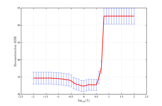
The minimization (17) is carried out using exhaustive search over the grid ${\cal L}$. Fig. 2 (right) shows how the reconstruction error $\hat{J}_{\textrm{rec}}(\cdot)$ is affected by the sparsity controlling coefficients. A simplified scenario is considered here with $\{\lambda_{\rho}=\lambda\}_{\rho=1}^{q}$, with $p=14$, and $q=r=2$. Matrix ${\mbox{\boldmath$\Sigma$}}_{x}={\mbox{\boldmath$\Sigma$}}_{s}$ is constructed so that $80\%$ of the ${\mathbf{U}}_{s}$ entries are zero. The black bars in Fig. 2 (right) quantify the standard error associated with each reconstruction MSE estimate in the red CV curve and its amplitude is calculated as

$$\textrm{Std}(\lambda)=\sqrt{n^{-1}}\sqrt{(n-1)^{-1}\sum_{t=1}^{n}[\hat{J}_{\textrm{rec}}^{m(t)}(\lambda)-\hat{J}_{\textrm{rec}}(\lambda)]^{2}}.$$ (18)

When $\lambda<0.1$ the reconstruction MSE remains almost constant and equal to the one achieved by standard PCA ($\lambda=0$). If $\lambda>10^{0.5}$, the reconstruction MSE increases and reaches a maximum equal to the trace of ${\mbox{\boldmath$\Sigma$}}_{x}$ (the DR and reconstruction matrices equal zero). The minimum MSE is achieved for $\lambda\approx 1$. Note that $\lambda_{\rho}$’s have so far been selected for a fixed value of $\mu$. Recall that $\mu$ controls the dissimilarity, of $\hat{{\mathbf{C}}}^{T}$ with $\hat{{\mathbf{B}}}$, thus a relatively large value ($\mu=100$ was used in the simulations) suffices to ensure that $\hat{{\mathbf{C}}}$ and $\hat{{\mathbf{B}}}$ stay close. Of course, the higher $\mu$ is the closer $\hat{{\mathbf{C}}}^{T}$ and $\hat{{\mathbf{B}}}$ will be.

IV S-PCA Properties

In this section sufficiently many training data are assumed available ($n\rightarrow\infty$), to allow analysis based on the ensemble covariance ${\mbox{\boldmath$\Sigma$}}_{x}={\mbox{\boldmath$\Sigma$}}_{s}+{\mbox{\boldmath$\Sigma$}}_{w}$. Recall that (a1) ensures a.s. convergence of the sample-based cost in (5) to its ensemble counterpart

$$({{\mathbf{B}}}_{e},{{\mathbf{C}}}_{e})\in\arg\min_{{\mathbf{B}},{\mathbf{C}}}\textrm{tr}[({\mathbf{I}}-{\mathbf{B}}{\mathbf{C}}){\mbox{\boldmath$\Sigma$}}_{x}({\mathbf{I}}-{\mathbf{B}}{\mathbf{C}})^{T}]+\sum_{\rho=1}^{q}\lambda_{\rho}(\|{\mathbf{C}}_{\rho:}^{T}\|_{1}+\|{\mathbf{B}}_{:\rho}\|_{1})+\mu\|{\mathbf{B}}-{\mathbf{C}}^{T}\|_{F}^{2}.$$ (19)

Interestingly, it will turn out that even in the presence of colored noise ${\mathbf{w}}_{t}$, the solution pair ${{\mathbf{B}}}_{e},{{\mathbf{C}}}_{e}$ can recover the support of the columns of the signal subspace ${\mathbf{U}}_{s,r}$, or at least part of it, as long as the noise power in ${\mathbf{x}}_{t}$ is sufficiently small.

IV-A Support recovery in colored noise

In this section entries of ${\mathbf{C}}_{e}$ (or ${\mathbf{B}}_{e}$) will be considered nonzero only if their corresponding magnitudes exceed an arbitrarily small threshold $\delta>0$. Under this condition it will be demonstrated next that for properly selected $\mu$ and $\lambda_{\rho}$, S-PCA assigns the (non)zero entries in ${\mathbf{C}}_{e}$ consistently with the support of the columns of ${\mathbf{U}}_{s,r}$. This means that the S-PCA formulation is meaningful because it does not assign entries of ${\mathbf{C}}_{e}$ (or ${\mathbf{B}}_{e}$) arbitrarily, but takes into account where the (non)zero entries of ${\mathbf{U}}_{s,r}$ are. Interestingly, this will hold even when colored noise is present, as long as its variance is properly upper bounded.

To proceed, let ${\mbox{\boldmath$\Sigma$}}_{s}$ be a permuted version of a block diagonal matrix. Specifically:
(a2) The entries of ${\mathbf{s}}$ can be partitioned into groups ${\cal G}_{1},\ldots,{\cal G}_{K}$, so that entries with indices in the same group are allowed to be correlated but entries with indices in different groups are uncorrelated; i.e., if $j\in{\cal G}_{k}$ and $j^{\prime}\in{\cal G}_{k^{\prime}}$, then $E[\mathbf{s}(j)\mathbf{s}(j^{\prime})]=0$ for $k\neq k^{\prime}$. Moreover, let $\{{\cal G}_{k}\}_{k=1}^{K}$ have the same cardinality that is equal to $G$. Using the proper permutation matrix $\mathbf{P}$, these groups can be made contiguous; hence, the vector $\mathbf{s}_{P}:=\mathbf{Ps}=[\mathbf{s}_{{\cal G}_{1}}\ldots\mathbf{s}_{{\cal G}_{K}}]^{T}$ has covariance matrix with block diagonal structure, that is $\mathbf{P}\mathbf{\Sigma}_{s}\mathbf{P}^{T}=\textrm{\emph{bdiag}}(\mathbf{\Sigma}_{{s}_{{\cal G}_{1}}},\ldots,\mathbf{\Sigma}_{{s}_{{\cal G}_{K}}})$. This implies that the eigenvector matrix $\tilde{\mathbf{U}}_{s}$ of $\mathbf{P}\mathbf{\Sigma}_{s}\mathbf{P}^{T}$ is block diagonal and sparse. Since $\mathbf{U}_{s}=\mathbf{P}^{T}\tilde{\mathbf{U}}_{s}$ and ${\mathbf{P}}$ is a permutation matrix, it follows that $\mathbf{U}_{s}$ is also sparse.
The block-diagonal structure under (a2) emerges when ${\mathbf{s}}_{t}$ corresponds e.g., to a random field in which the groups $\{{\cal G}_{k}\}_{k=1}^{K}$ correspond to different regions affected by groups of uncorrelated sources. Each of the sub-vectors ${\mathbf{s}}_{{\cal G}_{k}}$ in ${\mathbf{s}}_{P}$ contains sources affecting a certain region in the field and are uncorrelated from the other sources present in ${\mathbf{s}}_{P}$. It is worth stressing that (a2) does not prevent applicability of the ECD-SPCA (or BCD-SPCA) algorithm, but it is introduced here only to assess its asymptotic performance. Before stating the result proved in Appendix C, let ${\mathbf{v}}({\cal F})$ denote the entries of vector ${\mathbf{v}}$ with indices belonging to the set ${\cal F}$. Further, let ${\cal S}({\mathbf{v}})$ denote the support of ${\mathbf{v}}$, i.e., the set of indices of the nonzero entries of ${\mathbf{v}}$.

Proposition 1

Let ${\mbox{\boldmath$\Sigma$}}_{x}={\mbox{\boldmath$\Sigma$}}_{s}+{\mbox{\boldmath$\Sigma$}}_{w}$, with ${\mbox{\boldmath$\Sigma$}}_{s}$ satisfying (a2). Further, assume that the spectral radius of ${\mbox{\boldmath$\Sigma$}}_{w}$, namely $d_{\textrm{max}}({\mbox{\boldmath$\Sigma$}}_{w})$, satisfies $d_{\textrm{max}}({\mbox{\boldmath$\Sigma$}}_{w})<\Delta({\mbox{\boldmath$\Sigma$}}_{s})$, where $\Delta({\mbox{\boldmath$\Sigma$}}_{s})>0$ is a function of ${\mbox{\boldmath$\Sigma$}}_{s}$. If $\{\lambda_{\rho}=\lambda\}_{\rho=1}^{q}$ are selected such that $\|{{\mathbf{C}}}_{e,\rho:}\|_{0}\geq 2$, then for any arbitrarily small $\delta>0$ there exists a $\mu_{o}$ such that for any $\mu\geq\mu_{o}$ the minimization in (19) admits an optimal solution satisfying

$\displaystyle\|{\mathbf{C}}_{e,\rho:}^{T}(\bar{\cal S}_{i_{\rho}})\|_{1}\leq\delta,\;\textrm{\emph{and }}\|{\mathbf{C}}_{e,\rho:}^{T}({\cal S}_{i_{\rho}})\|_{1}\geq\xi(\lambda_{\rho})>0$ (20)
$\displaystyle\|{\mathbf{B}}_{e,:\rho}(\bar{\cal S}_{i_{\rho}})\|_{1}\leq\delta,\;\textrm{\emph{and }}\|{\mathbf{B}}_{e,:\rho}({\cal S}_{i_{\rho}})\|_{1}\geq\xi(\lambda_{\rho})>0,\;\;\textrm{ for }\rho=1,\ldots,q$ (21)

where $\bar{{\cal S}}_{i_{\rho}}$ is the complement of the support ${\cal S}_{i_{\rho}}$ of ${\mathbf{u}}_{s,i_{\rho}}$, while $\{i_{1},\ldots,i_{q}\}\subseteq\{1,\ldots,r\}$. The constant $\xi_{\rho}(\lambda_{\rho})$ depends only on $\lambda_{\rho}$ and is strictly positive for a finite $\lambda_{\rho}$.

Prop. 1 asserts that for $n$ sufficiently large, S-PCA has an optimal solution $({{\mathbf{B}}}_{e},{{\mathbf{C}}}_{e})$ whose support is a subset of the true support of $\{{\mathbf{u}}_{s,i_{\rho=1}}\}_{i=1}^{q}$ even in the presence of colored noise. This is possible since for the $\rho$th row of ${\mathbf{C}}_{e}$, there is a corresponding $i_{\rho}$ column of matrix ${\mathbf{U}}_{s,r}$ such that $\|{\mathbf{C}}_{e,\rho:}^{T}(\bar{\cal S}_{i_{\rho}})\|_{1}\leq\delta$ for arbitrarily small $\delta$, while $\|{\mathbf{C}}_{e,\rho:}^{T}({\cal S}_{i_{\rho}})\|_{1}\geq\xi_{\rho}(\lambda_{\rho})>\delta\geq 0$ (strictly positive). Thus, all the nonzero entries of ${\mathbf{C}}_{e,\rho:}^{T}$ with magnitude exceeding $\delta$ will have indices in ${\cal S}_{i_{\rho}}:=\textrm{support}({\mathbf{u}}_{s,i_{\rho}})$. This happens since: i) $\|{\mathbf{C}}_{e,\rho:}^{T}(\bar{\cal S}_{i_{\rho}})\|_{1}$ can be made arbitrarily small, thus all entries of ${\mathbf{C}}_{e,\rho:}^{T}$ with indices in $\bar{\cal S}_{i_{\rho}}$ can be driven arbitrarily close ($\delta$-close) to zero by controlling $\mu$; and ii) $\|{\mathbf{C}}_{e,\rho:}^{T}({\cal S}_{i_{\rho}})\|_{1}$ is strictly positive with $\xi_{\rho}(\lambda_{\rho})>\delta$, thus some of the entries of ${\mathbf{C}}_{e,\rho:}^{T}$ with indices in ${\cal S}_{i_{\rho}}$ must have magnitude greater than $\delta$. The number of nonzero entries in ${\mathbf{C}}_{e,\rho:}^{T}({\cal S}_{i_{\rho}})$ is determined by $\lambda_{\rho}$. Thus, if $\lambda_{\rho}$ is selected such that $\|{\mathbf{C}}_{e,\rho:}^{T}\|_{0}=\|{\mathbf{u}}_{s,i_{\rho}}\|_{0}$, then recovery of the whole support ${\cal S}_{i_{\rho}}$ is ensured.

Remark 2: It should be clarified that the vectors $\{{\mathbf{u}}_{s,i_{\rho}}\}_{\rho=1}^{q}$ in Prop. 1 may not all correspond to the $q$ principal eigenvectors of ${\mbox{\boldmath$\Sigma$}}_{s}$. Nonetheless S-PCA has an edge over standard PCA when colored noise corrupts the training data. If the observation noise is white, the eigenspaces of ${\mbox{\boldmath$\Sigma$}}_{x}$ and ${\mbox{\boldmath$\Sigma$}}_{s}$ coincide and the standard PCA will return the $q$ principal eigenvectors of ${\mbox{\boldmath$\Sigma$}}_{s}$. However, if ${\mathbf{w}}_{t}$ is colored the $q$ principal eigenvectors of ${\mbox{\boldmath$\Sigma$}}_{x}$, namely $\{{\mathbf{u}}_{x,\rho}\}_{\rho=1}^{q}$, will be different from $\{{\mathbf{u}}_{s,\rho}\}_{\rho=1}^{q}$ and may not be sparse. Actually, in standard PCA (cf. $\lambda_{\rho}=0$) the magnitude of $\|{\mathbf{C}}_{e,\rho:}^{T}(\bar{\cal S}_{i_{\rho}})\|_{1}$ depends on ${\mbox{\boldmath$\Sigma$}}_{w}$ and cannot be made arbitrarily small. Thus, the magnitude between the entries of ${\mathbf{C}}_{e,\rho:}^{T}$ with indices in $\bar{\cal S}_{i_{\rho}}$ relative to those those with indices in ${\cal S}_{i_{\rho}}$ cannot be controlled, for a given noise covariance matrix. This prevents one from discerning zero from nonzero entries in ${\mathbf{C}}_{e,\rho:}^{T}$, meaning that standard PCA cannot guarantee recovery even of a subset of the support of ${\mathbf{u}}_{s,i_{\rho}}$.

On the other hand, Prop. 1 states that S-PCA is capable of identifying a subset of (or all) the support index set of $\{{\mathbf{u}}_{s,i_{\rho}}\}_{\rho=1}^{q}$. S-PCA is more resilient to colored noise than standard PCA because it exploits the sparsity present in the eigenvectors of ${\mbox{\boldmath$\Sigma$}}_{s}$. Intuitively, the $\ell_{1}$ regularization terms act as prior information facilitating emergence of the ${\mathbf{U}}_{s,r}$ zero entries in ${\mathbf{C}}_{e}$ and ${\mathbf{B}}_{e}$ as long as the noise variance is not high. Although $\Delta({\mbox{\boldmath$\Sigma$}}_{s})$ has not been explicitly quantified, the upshot of Prop. 1 is that S-PCA is expected to estimate better the columns of ${\mathbf{U}}_{s,r}$ when compared to standard PCA under comparable noise power. Numerical tests will demonstrate that S-PCA achieves a smaller reconstruction MSE even in the presence of colored noise.

IV-B Oracle Properties

Turning now attention to the noiseless scenario (${\mbox{\boldmath$\Sigma$}}_{x}={\mbox{\boldmath$\Sigma$}}_{s}$), S-PCA is expected to perform satisfactorily as long as it estimates well the $q$ principal eigenvectors of ${\mbox{\boldmath$\Sigma$}}_{s}$. Reliable estimators of the clairvoyant matrices ${\mathbf{B}}_{o}={\mathbf{C}}_{o}^{T}={\mathbf{U}}_{s,q}^{T}$ can be obtained when a growing number of training vectors ensures that: i) the probability of identifying the zero entries of the eigenvectors approaches one; and also ii) the estimators of the non-zero entries of ${\mathbf{U}}_{s,q}$ satisfy a weak form of consistency [35]. Scaling rules for the $\lambda_{\rho}$’s will be derived to ensure that the S-PCA estimates $\hat{{\mathbf{B}}}$ and $\hat{{\mathbf{C}}}$ satisfy these so-termed oracle properties. The forthcoming results will be established for the BCD-SPCA scheme (of Sec. III-B), but similar arguments can be used to prove related claims for ECD-SPCA.

To this end, consider a weighted $\ell_{1}$-norm in (5), where the sparsity-controlling coefficient multiplying $|{\mathbf{B}}(j,\rho)|$ and $|{\mathbf{C}}(\rho,j)|$, namely $\lambda_{\rho,n}$, is replaced by the product $\hat{w}_{j,\rho,n}\lambda_{\rho,n}$. Note the dependence of $\lambda_{\rho,n}$ on $n$, while the $w$’s are set equal to $\hat{w}_{j,\rho,n}:=|\hat{{\mathbf{U}}}_{s,n}(j,\rho)|^{-\gamma}$, with $\gamma>0$ and $\hat{{\mathbf{U}}}_{s}$ denoting the estimate of ${\mathbf{U}}_{s}$ obtained via standard PCA. If ${\mathbf{U}}_{s}(j,\rho)$ is zero, then for $n$ sufficiently large the estimate $\hat{{\mathbf{U}}}_{s,n}(j,\rho)$ will have a small magnitude. This means large weight $\lambda_{\rho,n}\hat{w}_{j,\rho,n}$ and thus strongly encouraged sparsity in the corresponding estimates $\hat{{\mathbf{B}}}(j,\rho)$ and $\hat{{\mathbf{C}}}(\rho,j)$. The oracle properties for $\hat{{\mathbf{B}}}_{\tau,n}$ and $\hat{{\mathbf{C}}}_{\tau,n}$ are stated next and proved in Appendix D.

Proposition 2

Let $\hat{{\mathbf{C}}}_{\tau,n}$ in (8) be an asymptotically normal estimator of ${\mathbf{C}}_{o}={\mathbf{U}}_{s,q}^{T}$; that is,

$$\hat{{\mathbf{C}}}_{\tau,n}={\mathbf{U}}_{s,q}^{T}+\sqrt{n^{-1}}{{\mathbf{E}}}_{\tau,n}^{c}$$ (22)

where the $j$th column of ${{\mathbf{E}}}_{\tau,n}^{c}$ converges in distribution, as $n\rightarrow\infty$, to ${\cal N}(\mathbf{0},{\mbox{\boldmath$\Sigma$}}_{E_{c},j})$, i.e., a zero-mean Gaussian with covariance ${\mbox{\boldmath$\Sigma$}}_{E_{c},j}$. If the sparsity-controlling coefficients are chosen so that

$$\lim_{n\rightarrow\infty}\frac{\lambda_{\rho,n}}{\sqrt{n}}=0,\;\;\;\textrm{ and }\lim_{n\rightarrow\infty}\frac{\lambda_{\rho,n}}{n^{(1-\gamma)/2}}=\infty$$ (23)

then it holds under (a1) that (8) yields an asymptotically normal estimator of ${\mathbf{B}}_{o}={\mathbf{U}}_{s,q}$; that is,

$$\hat{{\mathbf{B}}}_{\tau,n}={\mathbf{U}}_{s,q}+\sqrt{n^{-1}}{{\mathbf{E}}}_{\tau,n}^{b}$$ (24)

where $\textrm{vec}({{\mathbf{E}}}_{\tau,n}^{b})({\cal S}_{o})\xrightarrow[n\rightarrow\infty]{d}{\cal N}(\mathbf{0},[{\mbox{\boldmath$\Sigma$}}_{E_{b}}]_{{\cal S}_{o}})$ (convergence in distribution); $[{\mbox{\boldmath$\Sigma$}}_{E_{b}}]_{{\cal S}_{o}}$ denotes the submatrix formed by the rows and columns, with indices in ${\cal S}_{o}:={\cal S}({\mathbf{U}}_{s,q})={\cal S}(\textrm{\emph{vec}}({\mathbf{U}}_{s,q}))$, of the error covariance ${\mbox{\boldmath$\Sigma$}}_{E_{b}}$ of $\textrm{vec}({{\mathbf{E}}}_{\tau,n}^{b})$ obtained when $\hat{{\mathbf{B}}}_{\tau,n}$ is evaluated by standard PCA. It follows that

$$\lim_{n\rightarrow\infty}\textrm{\emph{Pr}}[{\cal S}(\hat{{\mathbf{B}}}_{\tau,n})={\cal S}({\mathbf{U}}_{s,q})]=1.$$ (25)

Following similar arguments as in Prop. 2, it is possible to establish the following corollary.

Corollary 1

If $\hat{{\mathbf{B}}}_{\tau,n}$ is an asymptotically normal estimator of ${\mathbf{B}}_{o}$, and the sparsity-controlling coefficients are selected as in Prop. 2, then the optimal solution of (6) at iteration $\tau+1$, namely $\hat{{\mathbf{C}}}_{\tau+1,n}$, is an asymptotically normal estimator of ${\mathbf{C}}_{o}$ and $\lim_{n\rightarrow\infty}\textrm{\emph{Pr}}[{\cal S}(\hat{{\mathbf{C}}}_{\tau+1,n})={\cal S}({\mathbf{U}}_{s,q}^{T})]=1$.

Prop. 2 and Corollary 1 show that when the BCD-SPCA (or ECD-SPCA) is initialized properly and the sparsity-controlling coefficients follow the scaling rule in (23), then the iterates $\hat{{\mathbf{B}}}_{\tau,n}$ and $\hat{{\mathbf{C}}}_{\tau,n}$ satisfy the oracle properties for any iteration index $\tau$. This is important since it shows that the sparsity-aware estimators $\hat{{\mathbf{B}}}_{\tau,n}$ and $\hat{{\mathbf{C}}}_{\tau,n}$ achieve MSE performance which asymptotically is as accurate as that attained by a standard PCA approach for the nonzero entries of ${\mathbf{U}}_{s,q}$. This holds since the error covariance matrix of the estimates for the nonzero entries of ${\mathbf{U}}_{s,q}$, namely $[{\mbox{\boldmath$\Sigma$}}_{E_{b}}]_{{\cal S}_{o}}$, coincides with that corresponding to the standard PCA. The estimator $\hat{{\mathbf{B}}}_{0,n}=\hat{{\mathbf{C}}}_{0,n}^{T}=\hat{{\mathbf{U}}}_{s,q}$ obtained via standard PCA and used to initialize the BCD-SPCA and ECD-SPCA, is asymptotically normal [5, 19].

Remark 3: The scaling laws in (23) resemble those in [35, Thm. 2] for a linear regression problem. The difference here is that the estimate $\hat{{\mathbf{B}}}_{\tau-1,n}$ (or $\hat{{\mathbf{C}}}_{\tau,n}$) is nonlinearly related with $\hat{{\mathbf{C}}}_{\tau,n}$ ($\hat{{\mathbf{B}}}_{\tau,n}$ respectively). Thus, establishing Prop. 2 requires extra steps to account for the nonlinear interaction between $\hat{{\mathbf{C}}}_{\tau,n}$ and $\hat{{\mathbf{B}}}_{\tau,n}$. In order to show asymptotic normality, the chosen weights $\hat{w}_{j,\rho,n}$ are not that crucial. Actually, the part of the proof in Apdx. D that establishes asymptotic normality is valid also when, e.g., $\hat{w}_{j,\rho,n}=1$ and $\lim_{n\rightarrow\infty}{{n}}^{-1/2}{{\lambda_{\rho,n}}}=0$. However, the proposed weights $\hat{w}_{j,\rho,n}$ are instrumental when proving that the probability of recovering the ground-truth support of ${\mathbf{U}}_{s,q}$ converges to one as the number of training data grows large.

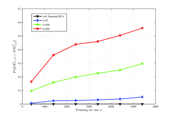
Although the probability of finding the correct support goes to one asymptotically as $n\rightarrow\infty$, numerical tests indicate that this probability is high even when $n$ and $\tau$ are finite. This is not the case for the standard PCA estimator, namely $\hat{{\mathbf{U}}}_{s,q,n}=\textrm{{q-principal eigenvecs}}(n^{-1}\sum_{t=1}^{n}{\mathbf{s}}_{t}{\mathbf{s}}_{t}^{T})$. Numerical examples will also demonstrate that even for a finite number of training data $n$, the probability of identifying the correct support is increasing as the coordinate descent iteration index $\tau$ increases. Thus, the signal subspace estimates obtained by BCD-SPCA (as well as ECD-SPCA) are capable of yielding the correct support of ${\mathbf{U}}_{s,q}$ even when $n$ is sufficiently large but finite. Consequently, improved estimates of ${\mathbf{U}}_{s,q}$ are obtained which explains the lower $J_{\textrm{rec}}({\mathbf{B}},{\mathbf{C}})$ attained by S-PCA relative to PCA.

V S-PCA Based transform coding

Up to this point sparsity has been exploited for DR of data vectors with analog-amplitude entries. However, the majority of modern compression systems are digital. This motivates incorporation of sparsity also in the quantization module that follows DR. This two-stage process comprises the transform coding (TC) approach which has been heavily employed in image compression applications due to its affordable computational complexity [16]. However, current TC schemes do not exploit the presence of sparsity that may be present in the covariance domain.

A sparsity-aware TC (SATC) is proposed here to complement the BCD-SPCA (or ECD-SPCA) algorithm during the data transformation step. The basic idea is to simply quantize the DR vectors using a VQ. Given ${\mathbf{x}}$, the DR matrix $\hat{{\mathbf{C}}}$ obtained by S-PCA is employed during the transformation step to produce the DR vector ${\mathbf{y}}=\hat{{\mathbf{C}}}{\mathbf{x}}$. Then, VQ is employed to produce at the output of the encoder a vector of quantized entries $\hat{{\mbox{\boldmath$\eta$}}}_{Q}=Q[{\mathbf{y}}]\in{\cal C}_{Q}^{q\times 1}$, where ${\cal C}_{Q}:=\{\hat{{\mbox{\boldmath$\eta$}}}_{1},\ldots,\hat{{\mbox{\boldmath$\eta$}}}_{L}\}$ is the quantizer codebook with cardinality $L=2^{R}$, where $R$ denotes the number of bits used to quantize ${\mathbf{y}}$. The VQ will be designed numerically using the Max-Lloyd algorithm, as detailed in e.g. [13], which uses $\{{\mathbf{y}}_{t}=\hat{{\mathbf{C}}}{\mathbf{x}}_{t}\}_{t=1}^{n}$ to determine the quantization cells $\{{\cal R}_{\hat{{\mbox{\boldmath$\eta$}}}_{l}}\}_{l=1}^{L}$, and their corresponding centroids, a.k.a. codewords $\{\hat{{\mbox{\boldmath$\eta$}}_{l}}\}_{l=1}^{L}$.

During decoding, the standard process in typical TC schemes [13, 16] is to multiply $\hat{{\mbox{\boldmath$\eta$}}}_{Q}=Q[\hat{{\mathbf{C}}}{\mathbf{x}}]$ with the matrix $(\hat{{\mathbf{C}}}^{T}\hat{{\mathbf{C}}})^{{\dagger}}\hat{{\mathbf{C}}}^{T}$, and form the estimate $\hat{{\mathbf{s}}}=(\hat{{\mathbf{C}}}^{T}\hat{{\mathbf{C}}})^{{\dagger}}\hat{{\mathbf{C}}}^{T}\hat{{\mbox{\boldmath$\eta$}}}_{Q}$. This estimate minimizes the Euclidean distance $\|\hat{{\mbox{\boldmath$\eta$}}}_{Q}-\hat{{\mathbf{C}}}{\mathbf{u}}\|$ wrt ${\mathbf{u}}$. Note that the reconstruction stage of SATC is also used in the DR setting considered in Sections II and III, except that $\hat{{\mbox{\boldmath$\eta$}}}_{Q}$ is replaced with the vector $\hat{{\mathbf{C}}}{\mathbf{x}}$ whose entries are analog. The reason behind using only $\hat{{\mathbf{C}}}$, and not $\hat{{\mathbf{B}}}$, is the penalty term $\|{\mathbf{B}}-{\mathbf{C}}^{T}\|_{F}^{2}$ which ensures that $\hat{{\mathbf{C}}}$ and $\hat{{\mathbf{B}}}^{T}$ will be close in the $\ell_{2}$-error sense. Certainly, $\hat{{\mathbf{B}}}$ could have been used instead, but such a change would not alter noticeably the reconstruction performance. Simulations will demonstrate that the sparsity-inducing mechanisms in the DR step assist SATC to achieve improved MSE reconstruction performance when compared to related sparsity-agnostic TCs.

VI Simulated Tests

Here the reconstruction performance of ECD-SPCA is studied and compared with the one achieved by standard PCA, as well as sparsity-aware alternatives that were modified to fit the dimensionality reduction setting. The different approaches are compared both in the noiseless and noisy scenarios. Simulation tests are also performed to corroborate the oracle properties established in Sec. IV-B. The SATC is compared with conventional TCs in terms of reconstruction MSE using synthetic data first. Then, SATC is tested in an image compression and denoising application using images from [1].

VI-A Synthetic Examples
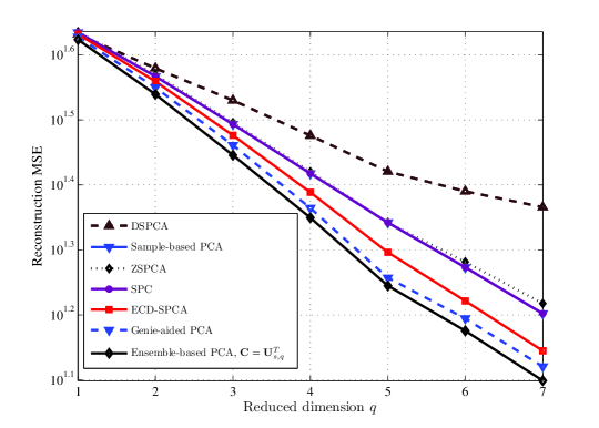
The reconstruction MSE $J_{\textrm{rec}}({\mathbf{B}}_{m},{\mathbf{C}}_{m})$ is measured for matrices ${{\mathbf{B}}}_{m}$ and ${{\mathbf{C}}}_{m}$ obtained via: i) ECD-SPCA; ii) the true signal subspace, i.e., $\mathbf{B}_{o}=\mathbf{C}_{o}^{T}={\mathbf{U}}_{s,q}$; iii) a ‘sample’-based PCA approach where $\hat{{\mathbf{U}}}_{x,q}$ is used; iv) a genie-aided PCA which relies on (iii) but also knows where the zero entries of $\mathbf{U}_{s,q}$ are located; v) the sparse PCA approach in [36] abbreviated as ZSPCA; vi) the scheme in [33] abbreviated as SPC; and vii) the algorithm of [9], which is abbreviated as DSPCA. With $p=14$ and $n=50$, the MSEs throughout the section are averaged over $200$ Monte Carlo runs using a data set that is different from the training set ${\mathbf{X}}$. In the noiseless case, ${\mbox{\boldmath$\Sigma$}}_{x}={\mbox{\boldmath$\Sigma$}}_{s}$ is constructed to be a permuted block diagonal matrix with $r=8$, while $80\%$ of the entries of ${\mathbf{U}}_{s,r}$ are zero. The sparsity-controlling coefficients multiplying $|{\mathbf{B}}(j,\rho)|$ and $|{\mathbf{C}}(\rho,j)|$ are set equal to ${\lambda_{\rho,n}}|\hat{{\mathbf{U}}}_{x}(i,j)|^{-\gamma}$, with $\gamma=1$ and $\lambda_{\rho,n}\sim n^{0.3}$. Fig. 3 (left) depicts $J_{\textrm{rec}}(\cdot)$ versus $q$. The sparsity coefficients in the sparsity-aware approaches are selected from a search grid to achieve the smallest possible reconstruction MSE. Clearly ECD-SPCA exploits the sparsity present in ${\mbox{\boldmath$\Sigma$}}_{s}$ and achieves a smaller reconstruction MSE that is very close to the genie-aided approach. Note that in Fig. 3 (left) there are seven curves. The curve corresponding to sample-based PCA almost overlaps with the one corresponding to SPC. It is also observed that the more sparse the eigenvectors in ${\mathbf{U}}_{s,r}$ are, the more orthogonal are the ECD-SPCA estimates $\hat{{\mathbf{B}}}$ and $\hat{{\mathbf{C}}}$. This suggests that the $\ell_{1}$ regularization terms in S-PCA induce approximate orthogonality in the corresponding estimates, as long as the underlying eigenvectors forming ${\mathbf{U}}_{s,r}$ are sufficiently sparse.

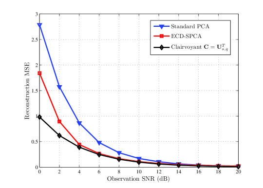
Fig. 3 (right) the reconstruction MSE is plotted as a function of the observation SNR, namely $\textrm{SNR}_{\textrm{obs}}:=10\log_{10}[\textrm{tr}({\mbox{\boldmath$\Sigma$}}_{s})/\textrm{tr}({\mbox{\boldmath$\Sigma$}}_{w})]$. The colored noise covariance matrix is factored as ${\mbox{\boldmath$\Sigma$}}_{w}={\mathbf{M}}_{w}{\mathbf{M}}_{w}^{T}$, where ${\mathbf{M}}_{w}$ is randomly generated matrix with Gaussian i.i.d. entries. The ECD-SPCA scheme is compared with the sparsity-agnostic standard PCA approach. With $r=q=3$ and $p=14$, ${\mbox{\boldmath$\Sigma$}}_{s}$ is constructed to be a permuted block diagonal matrix such that $70\%$ of the entries of the eigenmatrix ${\mathbf{U}}_{s,r}$ are equal to zero. All sparsity coefficients in ECD-SPCA are set equal to $\lambda=5*10^{-3}$. Fig. 3 (right) corroborates that the novel S-PCA can lead to better reconstruction/denoising performance than the standard PCA. The MSE gains are noticeable in the low-to-medium SNR regime. The sparsity imposing mechanisms of ECD-SPCA lead to improved subspace estimates yielding a reconstruction MSE that is close to the one obtained using ${\mathbf{U}}_{s,q}$. This result corroborates the claims of Prop. 1.

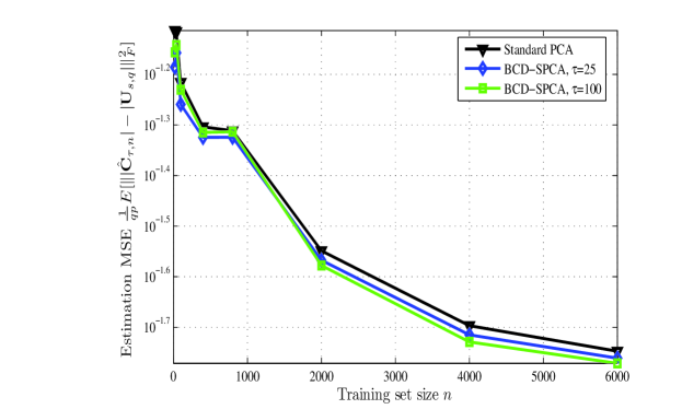
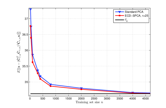
The next three figures validate the S-PCA properties in the noiseless case (see Sec. IV-B). Consider a setting where $p=14$, $r=8$, and $q=2$, and ${\mbox{\boldmath$\Sigma$}}_{x}={\mbox{\boldmath$\Sigma$}}_{s}$ constructed to be a permuted block diagonal matrix such that ${\mathbf{U}}_{s,r}$ has $70\%$ of its entries equal to zero. The $\lambda$’s are selected as in the first paragraph. Fig. 4 (left) displays the signal subspace estimation MSE $E[\||\hat{{\mathbf{C}}}_{\tau,n}|-|{\mathbf{U}}_{s,q}^{T}|\|_{F}^{2}]$, where the $|\cdot|$ operator is applied entry-wise and is used to eliminate any sign ambiguity present in the rows of $\hat{{\mathbf{C}}}_{\tau,n}$. As the training data size goes to infinity, the estimation error converges to zero. The convergence speed is similar to the one achieved by standard PCA. Similar conclusions can be deduced for the reconstruction MSE shown in Fig. 4 (right). The reconstruction MSE associated with ECD-SPCA is smaller than the one corresponding to standard PCA. The MSE advantage is larger for a small number of training data in which case standard PCA has trouble locating the zeros of ${\mathbf{U}}_{s,q}$. These examples corroborate the validity of Prop. 2. Interestingly, multiple coordinate descent iterations $(\tau>0)$ result in smaller estimation and reconstruction MSEs than the one achieved by standard PCA ($\tau=0$). The MSE gains are noticeable for a small number of training samples. Such gains are expected since ECD-SPCA (or BCD-SPCA) is capable of estimating the true support ${\cal S}({\mathbf{U}}_{s,q})$ with a positive probability even for a finite $n$. As shown in Fig. 5 (left), for $\tau>0$ the probability of finding the true support converges to one as $n\rightarrow\infty$ (cf. Prop. 2). As $\tau$ increases, this probability also increases, while standard PCA ($\tau=0$) never finds the correct support with a finite number of training data.

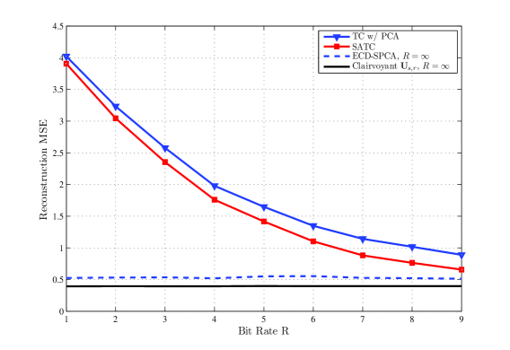
Next, the reconstruction MSE of the SATC (Sec.V) is considered and compared with the one achieved by a TC scheme based on standard PCA. The noisy setting used to generate Fig. 3 (right) is considered here with $p=14$ and $n=22$. With $r=q=3$, ${\mbox{\boldmath$\Sigma$}}_{s}$ is constructed to be a permuted block diagonal matrix so that $80\%$ of the entries of ${\mathbf{U}}_{s,r}$ are zero. Data reduction in SATC is performed via ECD-SPCA, while its sparsity controlling coefficients are set as described in the first paragraph of this section. Once the DR matrix $\hat{{\mathbf{C}}}$ is obtained, the DR training data $\hat{{\mathbf{C}}}{\mathbf{X}}$ are used to design the VQ using Max-Lloyd’s algorithm. Fig. 5 (right) depicts the reconstruction MSE versus the number of bits used to quantize a single DR vector. Fig. 5 (right) clearly shows that SATC benefits from the presence of sparsity in ${\mbox{\boldmath$\Sigma$}}_{s}$ and achieves improved reconstruction performance when compared to the standard TC scheme that relies on PCA. The dashed and solid lines correspond to the reconstruction MSE achieved by ECD-SPCA and ${\mathbf{U}}_{s,r}$ respectively while no quantization step is present ($R=\infty$).

VI-B Image compression and denoising

SATC is tested here for compressing and reconstructing images. These images have size $180\times 256$ and they are extracted, as described in Sec. II, from a bigger image of size $2520\times 2048$ in [1]. The images are corrupted with additive zero-mean Gaussian colored noise whose covariance ${\mbox{\boldmath$\Sigma$}}_{w}$ is structured as ${\mbox{\boldmath$\Sigma$}}_{w}={\mathbf{M}}{\mathbf{M}}^{T}$, where ${\mathbf{M}}$ contains Gaussian i.i.d. entries. The trace of ${\mbox{\boldmath$\Sigma$}}_{w}$ is scaled to fix the SNR at $15$dB. Out of a total of $112$ generated images, $30$ are used for training to determine the DR matrix $\hat{{\mathbf{C}}}$, and design the VQ. The rest are used as test images to evaluate the reconstruction performance of the following three schemes: i) the SATC; ii) a TC scheme that uses DCT; and iii) a TC scheme which relies on PCA.

The images are split into blocks of dimension $8\times 8$, and each of the three aforementioned TC schemes is applied to each block. Here $p=64$ and $\{{\mathbf{x}}_{t_{i}}\}_{i=1}^{30}$ is a vectorized representation of an $8\times 8$ sub-block that consists of certain image pixels, while $t_{i}\in\{1,\ldots,112\}$ denotes the image index. During the operational mode, datum ${\mathbf{x}}$ corresponds to a noisy sub-block occupying the same row and column indices as the ${\mathbf{x}}_{t_{i}}$’s but belonging to an image that is not in the training set. The signal of interest ${\mathbf{s}}$ corresponds to the underlying noiseless block we wish to recover. Each noisy datum ${\mathbf{x}}$ is transformed using either i) the SATC transformation matrix obtained via ECD-SPCA; or ii) the DCT; or iii) the PCA matrix. When the DCT is applied, then DR is performed by keeping the $q$ largest in magnitude entries of the transformed vector. The reduced dimension here is set to $q=14$. The $q\times 1$ vectors are further quantized by a VQ designed using the Max-Lloyd algorithm fed with the DR training vectors. At the decoder, the quantized vectors are used to reconstruct ${\mathbf{s}}$ by: i) using the scheme of Sec. V; ii) multiplying the quantized data with $\hat{{\mathbf{U}}}_{x,q}$ (PCA); or iii) applying inverse DCT to recover the original block. The sparsity-controlling coefficients in ECD-SPCA are all set equal to $\lambda=2*10^{-2}$.

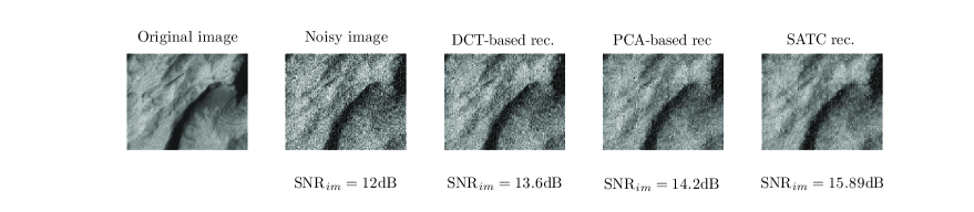
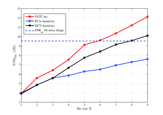
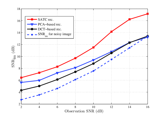
Fig. 6 shows: a) the original image; b) its noisy version; c) a reconstruction using DCT; d) a reconstruction using a PCA-based TC; and e) the reconstruction returned by SATC. The reconstructed images are obtained after setting the bit rate to $R=7$. The reconstruction returned by SATC is visually more pleasing than the one obtained by the DCT- and PCA-based TCs. The figure of merit used next is $\textrm{SNR}_{\textrm{im}}:=10log_{10}[\frac{P_{\textrm{signal}}}{P_{\textrm{error}}}]$, where $P_{\textrm{signal}}$ denotes the power of the noiseless image and $P_{\textrm{error}}$ the power of the noise present in the reconstructed image. Fig. 7 (left) displays $\textrm{SNR}_{\textrm{im}}$ versus the bit-rate of the VQ with SNR set at $17$dB. Clearly, SATC achieves higher $\textrm{SNR}_{\textrm{im}}$ values compared to the DCT- and PCA-based TCs. SATC performs better because the ECD-SPCA algorithm used to evaluate the DR matrix $\hat{{\mathbf{C}}}$ takes advantage of the sparsity present in ${\mbox{\boldmath$\Sigma$}}_{s}$. Similar conclusions can be drawn from Fig. 7 (right) depicting $\textrm{SNR}_{im}$ versus the SNR for $q=14$ and $R=7$ bits.

VII Concluding Remarks

The present work dealt with compression, reconstruction, and denoising of signal vectors spanned by an orthogonal set of sparse basis vectors that further result a covariance matrix with sparse eigenvectors. Based on noisy training data, a sparsity-aware DR scheme was developed using $\ell_{1}$-norm regularization to form improved estimates of the signal subspace leading to improved reconstruction performance. Efficient coordinate descent algorithms were developed to minimize the associated non-convex cost. The proposed schemes were guaranteed to converge at least to a stationary point of the cost.

Interesting analytical properties were established for the novel signal subspace estimator showing that even when the noise covariance matrix is unknown, a sufficiently large signal-to-noise ratio ensures that the proposed estimators identify (at least a subset) of the unknown support of the signal covariance eigenvectors. These results advocate that sparsity-aware compression performs well especially when a limited number of training data is available. Asymptotic normality is also established for the sparsity-aware subspace estimators, while it is shown that the probability of these estimates identifying the true signal subspace support approaches one as the number of training data grows large. Appropriate scaling laws for the sparsity-controlling coefficients were derived to satisfy the aforementioned properties.

Finally, the novel S-PCA approach was combined with vector quantization to form a sparsity-aware transform codec (SATC) that was demonstrated to outperform existing sparsity-agnostic approaches. Simulations using both synthetic data and images corroborated the analytical findings and validated the effectiveness of the proposed schemes. Work is underway to extend the proposed framework to settings involving compression of nonstationary signals, and processes with memory.

Acknowledgment

The authors would like to thank Prof. N. Sidiropoulos of the Technical University of Crete, Greece, for his valuable input and suggestions on the themes of this paper.

A. Proof of Lemma 1: The minimization problem in (12) can be equivalently expressed as

$$\hat{c}=\arg\min_{c}\|{\mbox{\boldmath$\chi$}}-c{\mathbf{h}}\|_{2}^{2}+\mu(c-\hat{b})^{2}+\lambda t,\;\;\;\textrm{s. to }-t\leq c\leq t$$ (26)

and the derivative of its Lagrangian function involving multipliers $\nu_{1}$ and $\nu_{2}$ is given by

$$\nabla_{c}{\cal L}(c,\nu_{1},\nu_{2})=2c{\mathbf{h}}^{T}{\mathbf{h}}-2c{\mathbf{h}}^{T}{\mbox{\boldmath$\chi$}}+2c\mu-2\mu\hat{b}+\nu_{1}-\nu_{2}.$$

After using the KKT necessary optimality conditions [3, pg. 316], it can be readily deduced that the optimal solution of (12) is given by the second equation in Lemma 1. $\square$

B. Proof of convergence of ECD-SPCA

Let $f(\{{\mathbf{B}}(j,\rho),{\mathbf{C}}(\rho,j)\}_{j=1,\rho=1}^{p,q})$ denote the S-PCA cost given in (5), defined over $\mathbb{R}^{2pq\times 1}$; and $f_{0}(\{{\mathbf{B}}(j,\rho),$ ${\mathbf{C}}(\rho,j)\}_{j=1,\rho=1}^{p,q}):=n^{-1}\|{\mathbf{X}}-{\mathbf{B}}{\mathbf{C}}{\mathbf{X}}\|_{F}^{2}+\mu\|{\mathbf{B}}-{\mathbf{C}}^{T}\|_{F}^{2}$. Next, consider the level set

$${\cal F}^{0}:=\{\{{\mathbf{B}}(j,\rho),{\mathbf{C}}(\rho,j)\}_{j=1,\rho=1}^{p,q}:\;\;f(\{{\mathbf{B}}(j,\rho),{\mathbf{C}}(\rho,j)\}_{j=1,\rho=1}^{p,q})\leq f(\hat{{\mathbf{B}}}_{0},\hat{{\mathbf{C}}}_{0})\}$$ (27)

where $\hat{{\mathbf{B}}}_{0}=\hat{{\mathbf{C}}}_{0}^{T}=\hat{{\mathbf{U}}}_{s,q}$ correspond to the matrices used to initialize ECD-SPCA obtained via standard PCA. If $\hat{{\mathbf{B}}}_{0}$ and $\hat{{\mathbf{C}}}_{0}$ have finite $\ell_{1}$-norms, the set ${\cal F}^{0}$ is closed and bounded (compact). The latter property can be deduced from (5) and (27), which ensure that matrices ${\mathbf{B}}$ and ${\mathbf{C}}$ in ${\cal F}^{0}$ satisfy $\sum_{\rho,j}\lambda_{\rho}(|{\mathbf{B}}(j,\rho)|+|{\mathbf{C}}(\rho,j)|\leq f(\hat{{\mathbf{B}}}_{0},\hat{{\mathbf{C}}}_{0})$. Moreover, $f(\hat{{\mathbf{B}}}_{0},\hat{{\mathbf{C}}}_{0})$ is finite when $\hat{{\mathbf{B}}}_{0}$ and $\hat{{\mathbf{C}}}_{0}$ have finite norms. This is true when the training data ${\mathbf{X}}$ contain finite entries. Thus, ${\cal F}^{0}$ is a compact set. Further, the cost function $f(\cdot)$ is continuous on ${\cal F}^{0}$.

From (11) and (14) it follows readily that the minimization problems solved to obtain $\hat{{\mathbf{C}}}_{\tau}(j,\rho)$ and $\hat{{\mathbf{B}}}_{\tau}(\rho,j)$, respectively, are strictly convex. Thus, minimizing $f(\cdot)$ with respect to an entry of ${\mathbf{C}}$ or ${\mathbf{B}}$ yields a unique minimizer, namely $\hat{{\mathbf{C}}}_{\tau}(\rho,j)$, or $\hat{{\mathbf{B}}}_{\tau}(j,\rho)$. Finally, $f(\cdot)$ satisfies the regularization conditions outlined in [30, (A1)]. Specifically, the domain of $f_{0}(\cdot)$ is formed by matrices whose entries satisfy ${\mathbf{B}}(j,\rho)\in(-\infty,+\infty)$ and ${\mathbf{C}}(\rho,j)\in(-\infty,+\infty)$ for $j=1,\ldots,p$ and $\rho=1,\ldots,q$. Thus, $\textrm{domain}(f_{0})=(-\infty,\infty)^{2qp}$ is an open set. Moreover, $f_{0}(\cdot)$ is G$\hat{\textrm{a}}$uteaux differentiable over $\textrm{domain}(f_{0})$. Specifically, the G$\hat{\textrm{a}}$uteaux derivative of $f_{0}(\cdot)$ is defined as

$$f_{0}^{\prime}({\mathbf{B}},{\mathbf{C}};{\mbox{\boldmath$\Delta$}}_{B},{\mbox{\boldmath$\Delta$}}_{C}):=\lim_{h\rightarrow 0}\frac{f_{0}({\mathbf{B}}+h{\mbox{\boldmath$\Delta$}}_{B},{\mathbf{C}}+h{\mbox{\boldmath$\Delta$}}_{C})-f_{0}({\mathbf{B}},{\mathbf{C}})}{h}.$$

Applying simple algebraic manipulations it follows readily that the G$\hat{\textrm{a}}$uteaux derivative exists for all ${\mbox{\boldmath$\Delta$}}_{B},{\mbox{\boldmath$\Delta$}}_{C}\in\textrm{domain}(f_{0})$, and is equal to $2\mu\textrm{tr}[({\mathbf{B}}-{\mathbf{C}}^{T})({\mbox{\boldmath$\Delta$}}_{B}-{\mbox{\boldmath$\Delta$}}_{C}^{T})^{T}]-2\textrm{tr}[({\mathbf{X}}-{\mathbf{B}}{\mathbf{C}}{\mathbf{X}})({\mbox{\boldmath$\Delta$}}_{B}{\mathbf{C}}{\mathbf{X}}+{\mathbf{B}}{\mbox{\boldmath$\Delta$}}_{C}{\mathbf{X}})^{T}]$. Then, convergence of the ECD-SPCA iterates to a stationary point of the S-PCA cost $f(\cdot)$ is readily established using [30, Thm. 4.1 (c)]. $\square$

C. Proof of Proposition 1: It can be shown by contradiction that for every $\epsilon>0$ there exists a $\mu_{\epsilon}$ such that for any $\mu>\mu_{\epsilon}$ it holds that $\|{{\mathbf{B}}}_{e}-{{\mathbf{C}}}_{e}^{T}\|_{1}\leq\epsilon/2$. Given that ${\mbox{\boldmath$\Sigma$}}_{x}={\mathbf{U}}_{x}{\mathbf{D}}_{x}{\mathbf{U}}_{x}^{T}$, and since $\|{{\mathbf{B}}}_{e}-{{\mathbf{C}}}^{T}_{e}\|_{1}<\epsilon/2$ for $\mu>\mu_{\epsilon}$, the minimization problem in (19) can be equivalently rewritten as

$${{\mathbf{C}}}_{e}(\epsilon)\in\arg\min_{{\mathbf{C}}}\textrm{tr}\left({\mathbf{D}}_{x}^{1/2}{\mathbf{U}}_{x}^{T}({\mathbf{I}}_{q}-2{\mathbf{C}}^{T}{\mathbf{C}}+{\mathbf{C}}^{T}{\mathbf{C}}{\mathbf{C}}^{T}{\mathbf{C}}){\mathbf{U}}_{x}{\mathbf{D}}_{x}^{1/2}\right)+\sum_{\rho=1}^{q}2\lambda\|{\mathbf{C}}_{\rho:}^{T}\|_{1}+\phi({\mathbf{C}},\epsilon,\mu)$$ (28)

where $\phi({\mathbf{C}},\epsilon,\mu)$ is a continuous function of ${\mathbf{C}}$ and $\epsilon$, while $\phi({\mathbf{C}},0,\mu)=0$.

Let us now consider how the support of each of the rows of ${{\mathbf{C}}}_{e}$ is related to the support of the principal eigenvectors $\{{\mathbf{u}}_{s,\rho}\}_{\rho=1}^{r}$. To this end, remove $\phi({\mathbf{C}},\epsilon,\mu)$ from (28) and consider the minimization problem

$$\check{{\mathbf{C}}}_{e}\in\arg\min_{{\mathbf{C}}}\textrm{tr}[({\mathbf{I}}-{\mathbf{C}}^{T}{\mathbf{C}}){\mbox{\boldmath$\Sigma$}}_{x}({\mathbf{I}}-{\mathbf{C}}^{T}{\mathbf{C}})^{T}]+\sum_{\rho=1}^{q}2\lambda\|{\mathbf{C}}_{\rho:}^{T}\|_{1}.$$ (29)

Since the cost in (28) is continuous, one recognizes after applying a continuity argument [11, pg. 15], that for any $\delta>0$ a sufficiently large $\mu_{\delta}$ can be found such that for any $\mu>\max(\mu_{\delta},\mu_{\epsilon})$ there exists an optimal solution ${{\mathbf{B}}}_{e},{{\mathbf{C}}}_{e}$ in (28), as well as an optimal solution $\check{{\mathbf{C}}}_{e}$ in (29) such that $\|{{\mathbf{C}}}_{e}-\check{{\mathbf{C}}}_{e}\|_{1}\leq\delta/2$ and $\|{{\mathbf{B}}}_{e}-\check{{\mathbf{C}}}_{e}^{T}\|_{1}\leq\|{{\mathbf{B}}}_{e}-{{\mathbf{C}}}_{e}^{T}\|_{1}+\|{{\mathbf{C}}}_{e}-\check{{\mathbf{C}}}_{e}\|_{1}\leq\delta$ (details are omitted due to space limitations). As the optimal solutions of (28) and (29) can be arbitrarily close, one considers the simpler of the two in (29).

Given that ${\mbox{\boldmath$\Sigma$}}_{x}={\mbox{\boldmath$\Sigma$}}_{s}+{\mbox{\boldmath$\Sigma$}}_{w}={\mathbf{U}}_{s,r}{\mathbf{D}}_{s,r}{\mathbf{U}}_{s,r}^{T}+{\mathbf{U}}_{w}{\mathbf{D}}_{w}{\mathbf{U}}_{w}^{T}$, the minimization in (29) can be rewritten as

$\displaystyle\tilde{{\mathbf{C}}}_{e}\in\arg\min_{\tilde{{\mathbf{C}}}}$ $\displaystyle\;\;\textrm{tr}\left(\tilde{{\mathbf{C}}}({\mbox{\boldmath$\Sigma$}}_{s,P}+{\mbox{\boldmath$\Sigma$}}_{w,P})\tilde{{\mathbf{C}}}^{T}(\tilde{{\mathbf{C}}}\tilde{{\mathbf{C}}}^{T}-2\mathbf{I}_{q})\right)+2\lambda\sum_{\rho=1}^{q}\|\tilde{{\mathbf{C}}}_{\rho:}^{T}\|_{1}$ (30)

where $\tilde{{\mathbf{C}}}={\mathbf{C}}{\mathbf{P}}^{T}$, ${\mbox{\boldmath$\Sigma$}}_{s,P}:={\mathbf{P}}{\mbox{\boldmath$\Sigma$}}_{s}{\mathbf{P}}^{T}$, ${\mbox{\boldmath$\Sigma$}}_{w,P}:={\mathbf{P}}{\mbox{\boldmath$\Sigma$}}_{w}{\mathbf{P}}^{T}$ while ${\mathbf{P}}$ is a permutation matrix constructed so that ${\mbox{\boldmath$\Sigma$}}_{s,P}$ is block diagonal, and $\tilde{{\mathbf{C}}}_{e}=\check{{\mathbf{C}}}_{e}{\mathbf{P}}^{T}$ denotes one of the optimal solutions of (30). Since the $\ell_{1}$-norm is permutation invariant, it holds that $\|{\mathbf{C}}_{\rho:}^{T}\|_{1}=\|\tilde{{\mathbf{C}}}_{\rho:}^{T}\|_{1}$.

The minimization problem in (30) can be equivalently written as

$\displaystyle\tilde{{\mathbf{C}}}_{e}\in\arg\min_{\tilde{{\mathbf{C}}}}$ $\displaystyle\;\;\textrm{tr}\left(\tilde{{\mathbf{C}}}{\mbox{\boldmath$\Sigma$}}_{x,P}\tilde{{\mathbf{C}}}^{T}(\tilde{{\mathbf{C}}}\tilde{{\mathbf{C}}}^{T}-2\mathbf{I}_{q})\right)+2\lambda\sum_{\rho=1}^{q}\sum_{j=1}^{p}{\mathbf{T}}(\rho,j),\textrm{ s. to }|\tilde{{\mathbf{C}}}(\rho,j)|\leq{\mathbf{T}}(\rho,j).$ (31)

Let ${\mathbf{T}}$ denote the $q\times p$ matrix whose $(\rho,j)$th entry is equal to ${\mathbf{T}}(\rho,j)$. Then, the Lagrangian of (31) is

$${\cal L}(\tilde{{\mathbf{C}}},{\mathbf{T}},{\mathbf{L}}_{1},{\mathbf{L}}_{2})=\textrm{tr}(\tilde{{\mathbf{C}}}{\mbox{\boldmath$\Sigma$}}_{x,P}\tilde{{\mathbf{C}}}^{T}(\tilde{{\mathbf{C}}}\tilde{{\mathbf{C}}}^{T}-2\mathbf{I}_{q}))+2\lambda\mathbf{1}_{q\times 1}^{T}{\mathbf{T}}\mathbf{1}_{p\times 1}+\textrm{tr}({\mathbf{L}}_{1}^{T}(\tilde{{\mathbf{C}}}-{\mathbf{T}}))+\textrm{tr}({\mathbf{L}}_{2}^{T}(-\tilde{{\mathbf{C}}}-{\mathbf{T}})),$$ (32)

where ${\mathbf{L}}_{1},{\mathbf{L}}_{2}\in\mathbb{R}^{q\times p}$ and their $(\rho,j)$th entry containts the Lagrange multiplier associated with the constraints $\tilde{{\mathbf{C}}}(\rho,j)\leq{\mathbf{T}}(\rho,j)$ and $-\tilde{{\mathbf{C}}}(\rho,j)\leq{\mathbf{T}}(\rho,j)$, respectively. The first-order optimality conditions imply that the gradient of ${\cal L}(\cdot)$ wrt $\tilde{{\mathbf{C}}}$ should be equal to zero when evaluated at $\tilde{{\mathbf{C}}}_{e}$, i.e.,

$$2\tilde{{\mathbf{C}}_{e}}\tilde{{\mathbf{C}}_{e}}^{T}\tilde{{\mathbf{C}}}_{e}{\mbox{\boldmath$\Sigma$}}_{x,P}+2\tilde{{\mathbf{C}}}_{e}{\mbox{\boldmath$\Sigma$}}_{x,P}\tilde{{\mathbf{C}}_{e}}^{T}\tilde{{\mathbf{C}}}_{e}-4\tilde{{\mathbf{C}}}_{e}{\mbox{\boldmath$\Sigma$}}_{x,P}+{\mathbf{L}}_{1}-{\mathbf{L}}_{2}=\mathbf{0}_{q\times p}.$$ (33)

Similarly, the gradient of ${\cal L}(\cdot)$ wrt ${\mathbf{T}}$ should be equal to zero at the optimum solution, ${\mathbf{T}}^{*}$, which leads to

$${\mathbf{L}}_{1}^{*}+{\mathbf{L}}^{*}_{2}=2\lambda\mathbf{1}_{q\times 1}\mathbf{1}^{T}_{p\times 1}.$$ (34)

Moreover, the optimal multipliers should be nonnegative, i.e., ${\mathbf{L}}_{1}^{*}(\rho,j)\geq 0$ and ${\mathbf{L}}_{2}^{*}(\rho,j)\geq 0$ for $j,\rho=1,\ldots,q$, while the complementary slackness conditions give that ${\mathbf{L}}_{1}^{*}(\rho,j)(\tilde{{\mathbf{C}}}_{e}(\rho,j)-T^{*}(\rho,j))=0$ and ${\mathbf{L}}_{2}^{*}(\rho,j)(-\tilde{{\mathbf{C}}}_{e}(\rho,j)-T^{*}(\rho,j))=0$ (see e.g., [3, pg. 316]).
Let ${\mathbf{e}}_{\rho}\in\mathbb{R}^{q\times 1}$ denote the canonical vector which has a single nonzero entry equal to one at the $\rho$-th position. After multiplying the left hand side (lhs) of (33) from the left with ${\mathbf{e}}_{\rho:}^{T}$ and from the right with $\tilde{{\mathbf{C}}}_{e,\rho:}$ we obtain

$\displaystyle 2\tilde{{\mathbf{C}}}_{e,\rho:}^{T}\tilde{{\mathbf{C}}}_{e}^{T}\tilde{{\mathbf{C}}}_{e}{\mbox{\boldmath$\Sigma$}}_{x,P}\tilde{{\mathbf{C}}}_{e,\rho:}+2\tilde{{\mathbf{C}}}_{e,\rho:}^{T}{\mbox{\boldmath$\Sigma$}}_{x,P}\tilde{{\mathbf{C}}}_{e}^{T}\tilde{{\mathbf{C}}}_{e}\tilde{{\mathbf{C}}}_{e,\rho:}$ $\displaystyle-4\tilde{{\mathbf{C}}}_{e,\rho:}^{T}{\mbox{\boldmath$\Sigma$}}_{x,P}\tilde{{\mathbf{C}}}_{e,\rho:}$ (35)
$\displaystyle\hskip 56.9055pt+\sum_{j=1}^{p}({\mathbf{L}}_{1}^{*}(\rho,j)-{\mathbf{L}}_{2}^{*}(\rho,j))\tilde{{\mathbf{C}}}_{e}(\rho,j)=0.$

Note that the last summand in (35) is equal to $2\lambda\|\tilde{{\mathbf{C}}}_{\rho:}\|_{1}$. This follows from the aforementioned slackness conditions. Specifically, if $\tilde{{\mathbf{C}}}_{e}(\rho,j)>0$ then $\tilde{{\mathbf{C}}}_{e}(\rho,j)={\mathbf{T}}^{*}({\rho,j})>0$, which further implies that ${\mathbf{L}}_{2}^{*}(\rho,j)=0$ and from (34) it follows that ${\mathbf{L}}_{1}^{*}(\rho,j)=2\lambda$. In the same way if $\tilde{{\mathbf{C}}}_{e}(\rho,j)<0$, then $\tilde{{\mathbf{C}}}_{e}(\rho,j)=-{\mathbf{T}}^{*}({\rho,j})<0$ from which it follows that ${\mathbf{L}}_{1}^{*}(\rho,j)=0$, thus from (34) we conclude that ${\mathbf{L}}_{2}^{*}(\rho,j)=2\lambda$. Thus, $({\mathbf{L}}_{1}^{*}(\rho,j)-{\mathbf{L}}_{2}^{*}(\rho,j))\tilde{{\mathbf{C}}}_{e}(\rho,j)=2\lambda|\tilde{{\mathbf{C}}}_{e}(\rho,j)|$, and after some algebraic manipulations on (35) it follows

$$\tilde{{\mathbf{C}}}_{e,\rho:}^{T}{\mbox{\boldmath$\Sigma$}}_{x,P}({\mathbf{I}}_{p\times p}-\tilde{{\mathbf{C}}}_{e}^{T}\tilde{{\mathbf{C}}}_{e})\tilde{{\mathbf{C}}}_{e,\rho:}=0.5\lambda\|\tilde{{\mathbf{C}}}_{e,\rho:}\|_{1},\;\;\rho=1,\ldots,q.$$ (36)

Summing the $q$ different equalities in (36) we obtain

$$\textrm{tr}({\mbox{\boldmath$\Sigma$}}_{x,P}({\mathbf{I}}_{p\times p}-\tilde{{\mathbf{C}}}_{e}^{T}\tilde{{\mathbf{C}}}_{e})\tilde{{\mathbf{C}}}_{e}^{T}\tilde{{\mathbf{C}}}_{e})=0.5\lambda\sum_{\rho=1}^{q}\|\tilde{{\mathbf{C}}}_{e,\rho:}\|_{1}$$ (37)

Equality (37) can be used to reformulate the cost in (30) without affecting the optimal solution. Specifically, the cost in (30) can be rewritten as $\textrm{tr}(\tilde{{\mathbf{C}}}{\mbox{\boldmath$\Sigma$}}_{x,P}\tilde{{\mathbf{C}}}^{T}\tilde{{\mathbf{C}}}\tilde{{\mathbf{C}}}^{T})-2\textrm{tr}(\tilde{{\mathbf{C}}}{\mbox{\boldmath$\Sigma$}}_{x,P}\tilde{{\mathbf{C}}}^{T})+2\lambda\sum_{\rho=1}^{q}\|\tilde{{\mathbf{C}}}_{\rho:}^{T}\|_{1}=-\textrm{tr}(\tilde{{\mathbf{C}}}{\mbox{\boldmath$\Sigma$}}_{x,P}\tilde{{\mathbf{C}}}^{T})+1.5\lambda\sum_{\rho=1}^{q}\|\tilde{{\mathbf{C}}}_{\rho,:}^{T}\|_{1}$. Using the latter cost expression and expanding the lhs of the $q$ different equality constraints in (36) the minimization problem in (30), is equivalent to

$\displaystyle\tilde{{\mathbf{C}}}_{e}\in\arg\min-\sum_{\rho=1}^{q}\tilde{{\mathbf{C}}}_{\rho:}^{T}{\mbox{\boldmath$\Sigma$}}_{x,P}\tilde{{\mathbf{C}}}_{\rho:}+1.5\lambda\sum_{\rho=1}^{q}\|\tilde{{\mathbf{C}}}_{\rho,:}^{T}\|_{1}$ (38)
$\displaystyle\textrm{s. to }\left(1-\|\tilde{{\mathbf{C}}}_{\rho:}\|_{2}^{2}\right)\tilde{{\mathbf{C}}}_{\rho:}^{T}{\mbox{\boldmath$\Sigma$}}_{x,P}\tilde{{\mathbf{C}}}_{\rho:}-\sum_{j=1,j\neq\rho}^{q}\left(\tilde{{\mathbf{C}}}_{j:}^{T}\tilde{{\mathbf{C}}}_{\rho:}\right)\left(\tilde{{\mathbf{C}}}_{\rho:}^{T}{\mbox{\boldmath$\Sigma$}}_{x,P}\tilde{{\mathbf{C}}}_{j:}\right)=0.5\lambda\|\tilde{{\mathbf{C}}}_{\rho:}\|_{1},\;{\rho=1},\ldots,{q}.$

Each one of the summands of the sum in the lhs of the equality constaints in (38) can be rewritten as

$$\tilde{{\mathbf{C}}}_{j:}^{T}\tilde{{\mathbf{C}}}_{\rho:}\tilde{{\mathbf{C}}}_{\rho:}^{T}{\mbox{\boldmath$\Sigma$}}_{x,P}\tilde{{\mathbf{C}}}_{j:}=\tilde{{\mathbf{C}}}_{\rho:}^{T}\left({\mbox{\boldmath$\Sigma$}}_{x,P}\tilde{{\mathbf{C}}}_{j:}\tilde{{\mathbf{C}}}_{j:}^{T}\right)\tilde{{\mathbf{C}}}_{\rho:}\geq 0,j,\rho=1,\ldots,q\textrm{ and }\rho\neq j.$$ (39)

Notice that the quantity in (39) is nonnegative since $\textrm{rank}({\mbox{\boldmath$\Sigma$}}_{x,P}\tilde{{\mathbf{C}}}_{j:}\tilde{{\mathbf{C}}}_{j:}^{T})=1$, while the single nonzero eigenvalue of ${\mbox{\boldmath$\Sigma$}}_{x,P}\tilde{{\mathbf{C}}}_{j:}\tilde{{\mathbf{C}}}_{j:}^{T}$ is $d_{\max}({\mbox{\boldmath$\Sigma$}}_{x,P}\tilde{{\mathbf{C}}}_{j:}\tilde{{\mathbf{C}}}_{j:}^{T})=\textrm{tr}({\mbox{\boldmath$\Sigma$}}_{x,P}\tilde{{\mathbf{C}}}_{j:}\tilde{{\mathbf{C}}}_{j:}^{T})=\tilde{{\mathbf{C}}}_{j:}^{T}{\mbox{\boldmath$\Sigma$}}_{x,P}\tilde{{\mathbf{C}}}_{j:}>0$ for $\tilde{{\mathbf{C}}}_{j:}\neq 0$. From the constraints in (38) and (39), it follows that $\|\tilde{{\mathbf{C}}}_{\rho:}\|_{2}\leq 1$, otherwise $\|\tilde{{\mathbf{C}}}_{\rho:}\|_{1}$ would be negative resulting a contradiction.

For the time being let us ignore the noise covariance matrix ${\mbox{\boldmath$\Sigma$}}_{w,P}$ by setting it to zero, thus ${\mbox{\boldmath$\Sigma$}}_{x,P}={\mbox{\boldmath$\Sigma$}}_{s,P}$. For the selected sparsity-controlling coefficient $\lambda$ in (30) assume that the optimal solution has $\|\tilde{{\mathbf{C}}}_{e,\rho:}^{T}\|_{0}=l_{\rho}$ and $\|\tilde{{\mathbf{C}}}_{e,\rho:}^{T}\|_{1}=\kappa_{\rho}$, while $2\leq l_{\rho}\leq G$ for $\rho=1,\ldots,q$. This is possible since the $\ell_{1}$-norm is used in S-PCA. The case $q=1$ is considered first to demonstrate the main result which is then generalized for $q>1$. Toward this end, let $\tilde{{\mathbf{C}}}_{1:}=\|\tilde{{\mathbf{C}}}_{1:}\|_{2}^{2}\cdot\mathbf{u}_{\tilde{c},:1}$, where $\|\mathbf{u}_{\tilde{c},:1}\|_{2}=1$. Moreover, to simplify notation let $c_{1}=\|\tilde{{\mathbf{C}}}_{1:}\|_{2}^{2}$, and $\gamma_{1}=\mathbf{u}_{\tilde{c},:1}^{T}{\mbox{\boldmath$\Sigma$}}_{s,P}\mathbf{u}_{\tilde{c},:1}$; thus $\tilde{{\mathbf{C}}}_{1:}^{T}{\mbox{\boldmath$\Sigma$}}_{s,P}\tilde{{\mathbf{C}}}_{1:}=c_{1}^{2}\gamma_{1}\geq 0$. Let $d_{1}^{*}$ denote the maximum spectral radius among all possible $l_{1}\times l_{1}$ submatrices of ${\mbox{\boldmath$\Sigma$}}_{s,P}$ that are formed after keeping $l_{1}$ of its rows and columns with common indices that are determined by the indices of the $l_{1}$ nonzero entries in the optimal $\tilde{{\mathbf{C}}}_{e,1:}=\|\tilde{{\mathbf{C}}}_{e,1:}\|_{2}^{2}\mathbf{u}_{\tilde{c},e,:1}$, and ${\mathbf{u}}_{\tilde{c},e,:1}$ the optimal selection for ${\mathbf{u}}_{\tilde{c},:1}$. Then, it holds that $\gamma_{1}=\mathbf{u}_{\tilde{c},:1}^{T}{\mbox{\boldmath$\Sigma$}}_{s,P}\mathbf{u}_{\tilde{c},:1}\leq d_{1}^{*}$ for any unit-vector $\mathbf{u}_{\tilde{c},:1}$ for which $\|\mathbf{u}_{\tilde{c},:1}\|_{0}=l_{1}$. With this notation in mind, $q=1$ and $\|\tilde{{\mathbf{C}}}_{e,1:}^{T}\|_{1}=\kappa_{1}$ (38) is equivalent to

$$\min_{c_{1},\gamma_{1}}-c^{2}_{1}\gamma_{1},\;\;\;\textrm{s. to }(1-c_{1}^{2})c_{1}^{2}\gamma_{1}=0.5\lambda\kappa_{1},\;\;0\leq c_{1}\leq\kappa_{1}^{\prime}=\min(1,\kappa_{1}),\;\;0\leq\gamma_{1}\leq d_{1}^{*},$$ (40)

where the first inequality constraint in (40) follows from the fact that $c_{1}\leq 1$ and $c_{1}=\|\tilde{{\mathbf{C}}}_{1:}\|_{2}<\kappa_{1}=\|\tilde{{\mathbf{C}}}_{1:}\|_{1}$. The Lagrangian of (40) is given as

$${\cal L}_{1}(c_{1},\gamma_{1},{\mathbf{v}})=-c^{2}_{1}\gamma_{1}+v_{1}^{a}[(1-c_{1}^{2})c_{1}^{2}\gamma_{1}-0.5\lambda\kappa_{1}]+v_{1}^{b}[c_{1}-\kappa_{1}^{\prime}]-v_{1}^{c}c_{1}-v_{1}^{d}\gamma_{1}+v_{1}^{e}(\gamma_{1}-d_{1}^{*}),$$ (41)

where ${\mathbf{v}}:=[v_{1}^{a}\;v_{1}^{b}\;v_{1}^{c}\;v_{1}^{d}\;v_{1}^{e}]^{T}$ contains the Lagrange multipliers. After i) differentiating (41) with respect to $c_{1}$ and $\gamma_{1}$; ii) setting the corresponding derivatives equal to zero; and iii) applying the complementary slackness conditions [see also Karush-Kuhn-Tucker necessary optimality condition in [3, pg. 316]] it follows that the optimal value $v_{1}^{e,*}$ of the multiplier $v_{1}^{e}$ should be strictly positive. The slackness conditions imply that $v_{1}^{e,*}(\gamma_{1}^{*}-d_{1}^{*})=0$, then it follows that at the minimum of (40) it holds that $\gamma_{1}^{*}=d_{1}^{*}$. Now recall that $\gamma_{1}=\mathbf{u}_{\tilde{c},:1}^{T}{\mbox{\boldmath$\Sigma$}}_{s,P}\mathbf{u}_{\tilde{c},:1}$, thus $\gamma_{1}^{*}$ is formed when $\mathbf{u}_{\tilde{c},:1}=\mathbf{u}_{\tilde{c},e,:1}$ (the optimal direction toward which the optimal row ${\mathbf{C}}_{e,\rho:}$ is pointing).

Recall that $d_{1}^{*}=\max_{{\mathbf{u}}_{\tilde{c},:1}}\mathbf{u}_{\tilde{c},:1}^{T}{\mbox{\boldmath$\Sigma$}}_{s,P}\mathbf{u}_{\tilde{c},:1}$ subject to $\|\mathbf{u}_{\tilde{c},:1}\|_{2}=1$ and $\|\mathbf{u}_{\tilde{c},:1}\|_{0}=l_{1}$. Next, we demonstrate that if $\mathbf{u}_{\tilde{c},e,:1}^{T}{\mbox{\boldmath$\Sigma$}}_{s,P}\mathbf{u}_{\tilde{c},e,:1}=d_{1}^{*}$, then there exists a column, say the $i_{1}$th in $\tilde{{\mathbf{U}}}_{s,r}$, with support $\tilde{{\cal S}}_{i_{1}}$ such that $\|{\mathbf{u}}_{\tilde{c},e,:1}^{T}(\bar{\tilde{{\cal S}}}_{i_{1}})\|_{1}=0$, while $\|{\mathbf{u}}_{\tilde{c},e,:1}^{T}(\tilde{\cal S}_{i_{1}})\|_{1}>0$ and $\bar{\tilde{{\cal S}}}_{i_{1}}$ denotes the complement of $\tilde{{\cal S}}_{i_{1}}$. Since $\tilde{{\mathbf{C}}}_{e,1:}^{T}$ is a scaled version of ${\mathbf{u}}_{\tilde{c},e,:1}^{T}$, the latter property will further imply that $\|\tilde{{\mathbf{C}}}_{e,1:}^{T}(\bar{\tilde{{\cal S}}}_{i_{1}})\|_{1}=0$, while $\|\tilde{{\mathbf{C}}}_{e,1:}^{T}(\tilde{\cal S}_{i_{1}})\|_{1}\geq\xi_{1}^{\prime}(\lambda)$, where $\xi_{1}^{\prime}(\lambda)$ is strictly positive. Equivalently, we will show that ${\cal I}_{1}:={\cal S}(\tilde{{\mathbf{C}}}_{e,1:})={\cal S}({{\mathbf{u}}}_{\tilde{c},e,:1})\subseteq{\cal G}_{k_{1}}$, where ${\cal G}_{k_{1}}=\tilde{{\cal S}}_{i_{1}}$ corresponds to the index set of the entries of ${\mathbf{s}}_{P}={\mathbf{P}}{\mathbf{s}}$ that belong to, say the $k_{1}$th diagonal block of ${\mbox{\boldmath$\Sigma$}}_{s,P}$ and $k_{1}\in\{1,\ldots,K\}$. To this end, let ${\mathbf{u}}_{\tilde{c},:1}^{T}=[({\mathbf{u}}_{\tilde{c},:1}^{1})^{T},$ $({\mathbf{u}}_{\tilde{c},:1}^{2})^{T},\ldots,({\mathbf{u}}_{\tilde{c},:1}^{K})^{T}]$, where each subvector ${\mathbf{u}}_{\tilde{c},:1}^{k}$ has $G$ entries; and let ${\cal I}_{1,k}:={\cal S}({\mathbf{u}}_{\tilde{c},:1}^{k})$ with $\sum_{k=1}^{K}|{\cal I}_{1,k}|=l_{1}$. Then, it follows that

$$\mathbf{u}_{\tilde{c},:1}^{T}{\mbox{\boldmath$\Sigma$}}_{s,P}\mathbf{u}_{\tilde{c},:1}=\sum_{k=1}^{K}({\mathbf{u}}_{\tilde{c},:1}^{k})^{T}{\mbox{\boldmath$\Sigma$}}_{s_{{\cal G}_{k}}}{\mathbf{u}}_{\tilde{c},:1}^{k}\leq\sum_{k=1}^{K}d_{\max}({\mbox{\boldmath$\Sigma$}}_{s_{{\cal G}_{k}}}^{l_{1}})\|{{\mathbf{u}}_{\tilde{c},:1}^{k}}\|_{2}^{2},$$ (42)

where $d_{\max}({\mbox{\boldmath$\Sigma$}}_{s_{{\cal G}_{k}}}^{l_{1}})$ denotes the spectral radius of the $l_{1}\times l_{1}$ submatrix ${\mbox{\boldmath$\Sigma$}}_{s_{{\cal G}_{k}}}^{l_{1}}$ formed by the $G\times G$ diagonal block ${\mbox{\boldmath$\Sigma$}}_{s_{{\cal G}_{k}}}$ of ${\mbox{\boldmath$\Sigma$}}_{x,P}$ after keeping $l_{1}$ of its rows and columns with common indices. The inequality in (42) follows since each subvector ${\mathbf{u}}_{\tilde{c},:1}^{k}$ of ${\mathbf{u}}_{\tilde{c},:1}$ can have at most $l_{1}$ nonzero entries. If $d_{1}^{l_{1}}$ denotes the maximum spectral radius that can be achieved by any $l_{1}\times l_{1}$ submatrix ${\mbox{\boldmath$\Sigma$}}_{s_{{}_{k}}}^{l_{1}}$ that is contained in a diagonal block ${\mbox{\boldmath$\Sigma$}}_{s_{{\cal G}_{k}}}$ of ${\mbox{\boldmath$\Sigma$}}_{s,P}$ for $k=1,\ldots,K$, then from (42) and since $\sum_{k=1}^{K}\|{\mathbf{u}}_{\tilde{c},:1}^{k}\|_{2}^{2}=1$ it holds that $\mathbf{u}_{\tilde{c},:1}^{T}{\mbox{\boldmath$\Sigma$}}_{s,P}\mathbf{u}_{\tilde{c},:1}\leq d_{1}^{l_{1}}$. Thus, it should hold that $d_{1}^{l_{1}}=d_{1}^{*}$. Then, the max value $d_{1}^{*}$ can be attained if and only if the indices of the nonzero entries of $\mathbf{u}_{\tilde{c},e,:1}$ satisfy ${\cal I}_{1}\subseteq{\cal G}_{k_{1}}$ for a $k_{1}\in\{1,\ldots,K\}$. This further implies that there exists an eigenvector $\tilde{{\mathbf{u}}}_{s,i_{1}}:={\mathbf{P}}{{\mathbf{u}}}_{s,i_{1}}$ with support $\tilde{{\cal S}}_{i_{1}}={\cal G}_{k_{1}}$, for which ${{\cal I}_{1}}\subseteq\tilde{{\cal S}}_{i_{1}}$. Thus, it is deduced that ${\mathbf{u}}_{\tilde{c},e,:1}^{T}(\bar{\tilde{{\cal S}}}_{i_{1}})=0$ and $\|{\mathbf{u}}_{\tilde{c},e,:1}^{T}(\tilde{\cal S}_{i_{1}})\|_{1}\geq\xi_{1}^{\prime}(\lambda)>0$ since the $l_{1}$ nonzero entries of ${\mathbf{u}}_{\tilde{c},e,:1}^{T}$ have indices in $\tilde{{\cal S}}_{i_{1}}$. Positivity of $\xi_{1}^{\prime}(\lambda)$ is ensured since $\|{\mathbf{u}}_{\tilde{c},e,:1}^{T}\|_{2}=1$ and $\lambda$ is selected such that $\tilde{{\mathbf{C}}}_{e,1:}=(c_{1}^{*})^{2}{\mathbf{u}}_{\tilde{c},e,:\rho}\neq\mathbf{0}$. Since $\check{{\mathbf{C}}}_{e}=\tilde{{\mathbf{C}}}_{e}{\mathbf{P}}$ in (29) results from permuting the columns of $\tilde{{\mathbf{C}}}_{e}$, it follows that $\|\check{{\mathbf{C}}}_{e,1:}^{T}(\bar{{{\cal S}}}_{i_{\rho}})\|_{1}=0$ and $\|\check{{\mathbf{C}}}_{e,1:}^{T}({\cal S}_{i_{\rho}})\|_{1}\geq\xi_{1}^{\prime}(\lambda)>0$, where ${\cal S}_{i_{\rho}}={\cal S}({\mathbf{u}}_{s,i_{\rho}})$.

We generalize the previous claim for the case when $q>1$. As before we reexpress each of the rows of $\tilde{{\mathbf{C}}}$ as $\tilde{{\mathbf{C}}}_{\rho:}=\|\tilde{{\mathbf{C}}}_{\rho:}\|_{2}^{2}{\mathbf{u}}_{\tilde{c},:\rho}$, with $\|{\mathbf{u}}_{\tilde{c},:\rho}\|_{2}=1$ for $\rho=1,\ldots,q$. No other assumptions are imposed for the direction vectors ${\mathbf{u}}_{\tilde{c},:\rho}$. Further, let $c_{\rho}=\|\tilde{{\mathbf{C}}}_{\rho:}\|_{2}$ and $\gamma_{\rho}={\mathbf{u}}_{\tilde{c},:\rho}^{T}{\mbox{\boldmath$\Sigma$}}_{s,P}{\mathbf{u}}_{\tilde{c},:\rho}$, where $\rho=1,\ldots,q$. Moreover, let $\delta_{j,\rho}=({\mathbf{u}}_{\tilde{c},:j}^{T}{\mathbf{u}}_{\tilde{c},:\rho})({\mathbf{u}}_{\tilde{c},:j}^{T}{\mbox{\boldmath$\Sigma$}}_{s,P}{\mathbf{u}}_{\tilde{c},:\rho})$ for $j\neq\rho$ and further notice that $\delta_{j,\rho}=\delta_{\rho,j}\geq 0$ [cf. (39)], while $\delta_{j,\rho}\leq\gamma_{\rho}$ and $\delta_{j,\rho}\leq\gamma_{j}$. Also recall that $\lambda$ has been selected such that $\{\|\tilde{{\mathbf{C}}}_{e,\rho:}\|_{1}=\kappa_{\rho}\}_{\rho=1}^{q}$ and $\{\|\tilde{{\mathbf{C}}}_{e,\rho:}\|_{0}=l_{\rho}\}_{\rho=1}^{q}$ where $2\leq l_{\rho}\leq G$. Then, the minimization problem in (38) can be equivalently rewritten as

$\displaystyle\min-\sum_{\rho=1}^{q}c_{\rho}^{2}\gamma_{\rho},\;\;\;$ $\displaystyle\textrm{s. to }(1-c_{\rho}^{2})c_{\rho}^{2}\gamma_{\rho}-\sum_{j=1,j\neq\rho}^{q}c_{\rho}^{2}c_{j}^{2}\delta_{j,\rho}=0.5\lambda\kappa_{\rho},\;,0\leq c_{\rho}\leq\kappa_{\rho}^{\prime}:=\min(1,\kappa_{\rho})\;$
$\displaystyle 0\leq\gamma_{\rho}\leq d_{\rho}^{*},\;\;,0\leq\delta_{j,\rho}\leq\gamma_{\rho},\;\;\delta_{j,\rho}\leq\gamma_{j},\;\;\delta_{j,\rho}=\delta_{\rho,j},\;j\neq\rho,\;j,\rho=1,\ldots,q$ (43)

where $d_{\rho}^{*}$ corresponds to the maximum value that ${\mathbf{u}}_{\tilde{c},\rho:}^{T}{\mbox{\boldmath$\Sigma$}}_{x,P}{\mathbf{u}}_{\tilde{c},\rho:}$ can attain when $\|\tilde{{\mathbf{C}}}_{\rho:}\|_{0}=l_{\rho}$, while ${\mathbf{u}}_{\tilde{c},\rho:}$ are selected such that the constraints in (Acknowledgment) are satisfied. The Lagrangian function of (Acknowledgment) is given as

$\displaystyle{\cal L}_{2}(\{c_{\rho},\gamma_{\rho}\}_{\rho=1}^{q},\{\delta_{j,\rho}\},{\mathbf{v}})=$ $\displaystyle-\sum_{\rho=1}^{q}c_{\rho}^{2}\gamma_{\rho}+\sum_{\rho=1}^{q}v_{\rho}^{a}[(1-c_{\rho}^{2})c_{\rho}^{2}\gamma_{\rho}-\sum_{j=1,j\neq\rho}^{q}c_{\rho}^{2}c_{j}^{2}\delta_{j,\rho}-0.5\lambda\kappa_{\rho}]$ (44)
$\displaystyle+\sum_{\rho=1}^{q}\left[v_{\rho}^{b}(c_{\rho}-\kappa_{\rho}^{\prime})-v_{\rho}^{c}c_{\rho}+v_{\rho}^{d}(\gamma_{\rho}-d_{\rho}^{*})-v_{\rho}^{e}\gamma_{\rho}\right]$
$\displaystyle+\sum_{\rho=1}^{q}\sum_{j=1,j\neq\rho}^{q}\left[v_{j,\rho}^{f}(\delta_{j,\rho}-\gamma_{\rho})+v_{j,\rho}^{g}(\delta_{j,\rho}-\gamma_{j})+v_{j,\rho}^{h}(\delta_{j,\rho}-\delta_{\rho,j})-v_{j,\rho}^{i}\delta_{j,\rho}\right],$

where ${\mathbf{v}}$ is a vector that contains the Lagrange multipliers $v_{\rho}^{a},v_{\rho}^{b},v_{\rho}^{c},v_{\rho}^{d},v_{\rho}^{e},v_{j,\rho}^{f},v_{j,\rho}^{g}$, $v_{j,\rho}^{h}$ and $v_{j,\rho}^{i}$. The KKT conditions are applied next to derive necessary conditions that the optimal solution of (Acknowledgment) should satisfy. This involves i) differentiating (44) wrt $c_{\rho}$, $\gamma_{\rho}$ and $\delta_{j,\rho}$; ii) setting the corresponding derivatives equal to zero; and iii) applying the complementary slackness conditions for the optimal multipliers ${\mathbf{v}}^{*}$. Then, it follows that at the minimum of (Acknowledgment) it should hold that $\delta_{j,\rho}^{*}=0$, and $\gamma_{\rho}^{*}=d_{\rho}^{*}$ for $j,\rho=1,\ldots,q$ and $j\neq\rho$. From the definition of $\delta_{j,\rho}$ it follows that $\delta_{j,\rho}^{*}$ is formed using the optimal vectors ${\mathbf{u}}_{\tilde{c},e,\rho:}$, i.e., $\delta_{j,\rho}^{*}=({\mathbf{u}}_{\tilde{c},e,:j}^{T}{\mathbf{u}}_{\tilde{c},e,:\rho})({\mathbf{u}}_{\tilde{c},e,:j}^{T}{\mbox{\boldmath$\Sigma$}}_{s,P}{\mathbf{u}}_{\tilde{c},e,:\rho})$. Since $\delta_{j,\rho}^{*}=0$, it follows that the optimal direction vector ${\mathbf{u}}_{\tilde{c},e,:\rho}$ should be selected in (38) such that ${\mathbf{u}}_{\tilde{c},e,:j}^{T}{\mathbf{u}}_{\tilde{c},e,:\rho}=0$, or ${\mathbf{u}}_{\tilde{c},e,:j}^{T}{\mbox{\boldmath$\Sigma$}}_{s,P}{\mathbf{u}}_{\tilde{c},e,:\rho}=0$ for $j\neq\rho$, while $\gamma_{\rho}^{*}={\mathbf{u}}_{\tilde{c},e,:\rho}^{T}{\mbox{\boldmath$\Sigma$}}_{s,P}{\mathbf{u}}_{\tilde{c},e,:\rho}$ iis equal to the maximum possible value $d_{\rho}^{*}$. Since $\tilde{{\mathbf{C}}}_{e,\rho:}=(c_{\rho}^{*})^{2}{\mathbf{u}}_{\tilde{c},e,:\rho}$ it follows that the rows of the optimal matrix $\tilde{{\mathbf{C}}}_{e}$ should be selected such that either they are orthogonal $\tilde{{\mathbf{C}}}_{e,\rho:}^{T}\tilde{{\mathbf{C}}}_{e,j:}=0$, or $\tilde{{\mathbf{C}}}_{e,\rho:}^{T}{\mbox{\boldmath$\Sigma$}}_{s,P}\tilde{{\mathbf{C}}}_{e,j:}=0$. In summary the direction vector for the $\rho$th row of the optimal matrix $\tilde{{\mathbf{C}}}_{e}$ in (38), namely ${\mathbf{u}}_{\tilde{c},e,:\rho}$, should be selected such that

$${\mathbf{u}}_{\tilde{c},e,:\rho}=\arg\max_{{\mathbf{u}}_{\tilde{c},\rho:}}{\mathbf{u}}_{\tilde{c},:\rho}^{T}{\mbox{\boldmath$\Sigma$}}_{s,P}{\mathbf{u}}_{\tilde{c},:\rho},\;\;\;\textrm{s. to }({\mathbf{u}}_{\tilde{c},:j}^{T}{\mathbf{u}}_{\tilde{c},e,:\rho})({\mathbf{u}}_{\tilde{c},:j}^{T}{\mbox{\boldmath$\Sigma$}}_{s,P}{\mathbf{u}}_{\tilde{c},:\rho})=0,\;\;\|{\mathbf{u}}_{\tilde{c},:\rho}\|_{2}=1,\;\;\|{\mathbf{u}}_{\tilde{c},e,:\rho})\|_{1}=l_{\rho},$$

where $\rho=1,\ldots,q,\;j\neq\rho.$ Using similar reasoning as in the case where $q=1$ it follows that for every optimal row $\tilde{{\mathbf{C}}}_{e,\rho:}$ there exists $i_{\rho}\in\{1,\ldots,r\}$ such that ${\cal I_{\rho}}={\cal S}(\tilde{{\mathbf{C}}}_{e,\rho:}^{T})\subseteq{\cal S}(\tilde{{\mathbf{u}}}_{s,i_{\rho}})$ Letting $\bar{\tilde{{\cal S}}}_{i_{\rho}}$ be the complement of $\tilde{{\cal S}}_{i_{\rho}}$, it is deduced that ${\mathbf{u}}_{\tilde{c},e,:\rho}^{T}(\bar{\tilde{{\cal S}}}_{i_{\rho}})=0$ and $\|{\mathbf{u}}_{\tilde{c},e,\rho:}^{T}(\tilde{\cal S}_{i_{\rho}})\|_{1}\geq\xi_{\rho}^{\prime}(\lambda)>0$ since the $l_{\rho}$ nonzero entries of ${\mathbf{u}}_{\tilde{c},e,:\rho}^{T}$ have indices in $\tilde{{\cal S}}_{i_{\rho}}$. Positivity of $\xi_{\rho}^{\prime}(\lambda)$ is ensured since $\|{\mathbf{u}}_{\tilde{c},e,:\rho}^{T}\|_{2}=1$ and $\tilde{{\mathbf{C}}}_{e,\rho:}=(c_{\rho}^{*})^{2}{\mathbf{u}}_{\tilde{c},e,:\rho}\neq\mathbf{0}$ for the selected $\lambda$. Then, it follows readily that $\|\tilde{{\mathbf{C}}}_{e,\rho:}(\bar{\tilde{{\cal S}}}_{i_{\rho}})\|_{1}=0$ while $\|\tilde{{\mathbf{C}}}_{e,\rho:}(\tilde{\cal S}_{i_{\rho}})\|_{1}\geq\xi_{\rho}^{\prime}(\lambda)>0$ for $\rho=1,\ldots,q$. Since $\check{{\mathbf{C}}}_{e}=\tilde{{\mathbf{C}}}_{e}{\mathbf{P}}$ in (29) results from permuting the columns of $\tilde{{\mathbf{C}}}_{e}$ it follows that $\|\check{{\mathbf{C}}}_{e,\rho:}^{T}(\bar{{{\cal S}}}_{i_{\rho}})\|_{1}=0$ and $\|\check{{\mathbf{C}}}_{e,\rho:}^{T}({\cal S}_{i_{\rho}})\|_{1}\geq\xi_{\rho}^{\prime}(\lambda)>0$, where ${\cal S}_{i_{\rho}}={\cal S}({\mathbf{u}}_{s,i_{\rho}})$.

The latter property was proved under the assumption that ${\mbox{\boldmath$\Sigma$}}_{w,P}=0$. Consider now the general case where ${\mbox{\boldmath$\Sigma$}}_{w,P}\neq\mathbf{0}$, thus ${\mbox{\boldmath$\Sigma$}}_{x,P}\neq{\mbox{\boldmath$\Sigma$}}_{s,P}$. An upper bound on the noise variance will be determined that ensures the validity of the earlier claims about $\tilde{{\mathbf{C}}}_{e,\rho:}^{T}$ (or $\check{{\mathbf{C}}}_{e,\rho:}^{T}$) established in the noiseless case. Let $\check{{\mathbf{u}}}_{\tilde{c},:\rho}$ be a direction vector that results a row vector $\check{{\mathbf{C}}}_{\rho:}$ that belongs to the constraint set of (38), while $\|\check{{\mathbf{u}}}_{\tilde{c},:\rho}\|_{0}=\|\check{{\mathbf{C}}}_{\rho:}\|_{0}=l_{\rho}$. Further, assume that the support of $\check{{\mathbf{u}}}_{\tilde{c},:\rho}$ is different from the support of the optimal ${\mathbf{u}}_{\tilde{c},e,:\rho}^{T}$ evaluated when ${\mbox{\boldmath$\Sigma$}}_{w,P}=\mathbf{0}$. One sufficient condition to ensure optimality of $\{{\mathbf{u}}_{\tilde{c},e,:\rho}^{T}\}_{\rho=1}^{q}$ in the presence of noise is that

$$\check{{\mathbf{u}}}_{\tilde{c},:\rho}^{T}{\mbox{\boldmath$\Sigma$}}_{s,P}\check{{\mathbf{u}}}_{\tilde{c},:\rho}+\check{{\mathbf{u}}}_{\tilde{c},:\rho}^{T}{\mbox{\boldmath$\Sigma$}}_{w,P}\check{{\mathbf{u}}}_{\tilde{c},:\rho}<d^{*}_{\rho}={\mathbf{u}}_{\tilde{c},e,:\rho}^{T}{\mbox{\boldmath$\Sigma$}}_{s,P}{\mathbf{u}}_{\tilde{c},e,:\rho},\;\;\rho=1,\ldots,q.$$ (45)

for any $\check{{\mathbf{u}}}_{\tilde{c},:\rho}$ that results a feasible $\check{{\mathbf{C}}}_{\rho:}$ in (38), while $\|\check{{\mathbf{u}}}_{\tilde{c},:\rho}\|_{0}=l_{\rho}$ and ${\cal S}(\check{{\mathbf{u}}}_{\tilde{c},:\rho})\neq{\cal S}({\mathbf{u}}_{\tilde{c},e,:\rho})$. Given that $\check{{\mathbf{u}}}_{\tilde{c},:\rho}^{T}{\mbox{\boldmath$\Sigma$}}_{w,P}\check{{\mathbf{u}}}_{\tilde{c},:\rho}\leq d_{\textrm{max}}({\mbox{\boldmath$\Sigma$}}_{w,P})$, it follows that (45) will be satisfied when

$$d_{\textrm{max}}({\mbox{\boldmath$\Sigma$}}_{w,P})<d^{*}_{\rho}-\check{{\mathbf{u}}}_{\tilde{c},:\rho}^{T}{\mbox{\boldmath$\Sigma$}}_{s,P}\check{{\mathbf{u}}}_{\tilde{c},:\rho}.$$ (46)

Note that $\check{{\mathbf{u}}}_{\tilde{c},:\rho}^{T}{\mbox{\boldmath$\Sigma$}}_{s,P}\check{{\mathbf{u}}}_{\tilde{c},:\rho}<d^{*}_{\rho}$ since $\check{{\mathbf{u}}}_{\tilde{c},:\rho}$ does not have the same support as ${\mathbf{u}}_{\tilde{c},e,\rho:}^{T}$ that maximizes the problem at the bottom of pg. 28, in which ${\mbox{\boldmath$\Sigma$}}_{w,P}=\mathbf{0}$. Thus, the quantity in the right hand side of (46), denoted as $\Delta({\mbox{\boldmath$\Sigma$}}_{s})$, will be positive.

What remains to establish are the properties stated in Prop. 1 for ${\mathbf{C}}_{e,\rho:}^{T}$ and ${\mathbf{B}}_{e,:\rho}$ with $\rho=1,\ldots,q$. To this end, recall that for any $\mu>\max(\mu_{\delta},\mu_{\epsilon})$, and for each $\tilde{{\mathbf{C}}}_{e}$, or equivalently $\check{{\mathbf{C}}}_{e}$, there exists an optimal solution ${{\mathbf{C}}}_{e}$ and ${{\mathbf{B}}}_{e}$ of (19) for which $\|{{\mathbf{C}}}_{e}-\check{{\mathbf{C}}}_{e}\|_{1}\leq\delta/2$ and $\|{{\mathbf{B}}}_{e}-\check{{\mathbf{C}}}_{e}^{T}\|_{1}\leq\delta$, where $\check{{\mathbf{C}}}_{e}=\tilde{{\mathbf{C}}}_{e}{\mathbf{P}}$. Then, $\|{{\mathbf{C}}}_{e,\rho:}^{T}-\check{{\mathbf{C}}}_{e}\|_{1}\leq\delta/2$ for $\rho=1,\ldots,q$. Then, it readily follows that $\|{{\mathbf{C}}}_{e,\rho:}^{T}(\bar{\cal S}_{i_{\rho}})\|_{1}\leq\delta/2$ since $\check{{{\mathbf{C}}}}_{e,\rho:}^{T}(\bar{\cal S}_{i_{\rho}})=\mathbf{0}^{T}$. Moreover, $\|\check{{{\mathbf{C}}}}_{e,\rho:}^{T}({\cal S}_{i_{\rho}})\|-\delta/2\leq\|{{\mathbf{C}}}_{e,\rho:}^{T}({\cal S}_{i_{\rho}})\|_{1}\leq\|\check{{{\mathbf{C}}}}_{e,\rho:}^{T}({\cal S}_{i_{\rho}})\|+\delta/2$. Notice that the lower bound $\|\check{{{\mathbf{C}}}}_{e,\rho:}^{T}({\cal S}_{i_{\rho}})\|-\delta/2\geq\xi_{\rho}^{\prime}(\lambda)-\delta/2$ can be made strictly positive by pushing $\delta/2$ arbitrarily close to zero, which is possible by increasing $\mu$. However, $\xi_{\rho}(\lambda)$ remains strictly positive for the values of $\lambda_{\rho}$ considered here, since it does not depend on $\mu$. These properties can also be established for ${\mathbf{B}}_{e,:\rho}$ using similar arguments. $\square$

D. Proof of Proposition 2: In the noiseless case the training matrix ${\mathbf{X}}_{n}={\mathbf{S}}_{n}$ (note the dependence on $n$) can be written as ${\mathbf{S}}_{n}={\mathbf{U}}_{s,q}{\mathbf{U}}_{s,q}^{T}{\mathbf{S}}_{n}+{\mathbf{U}}_{s,p-q}{\mathbf{U}}_{s,p-q}^{T}{\mathbf{S}}_{n}$. For notational convenience let ${\mbox{\boldmath$\Gamma$}}_{q,n}={\mathbf{U}}_{s,q}^{T}{\mathbf{S}}_{n}$, and ${\mathbf{z}}_{q,n}=\textrm{vec}({\mathbf{U}}_{s,p-q}$ ${\mathbf{U}}_{s,p-q}^{T}{\mathbf{S}}_{n})=\left(({\mathbf{U}}_{s,p-q}^{T}{\mathbf{S}}_{n})^{T}\otimes{\mathbf{I}}_{p}\right)\textrm{vec}({\mathbf{U}}_{s,p-q})$. Using vec notation, it holds that $\textrm{vec}({\mathbf{S}}_{n})=({\mbox{\boldmath$\Gamma$}}_{q,n}^{T}\otimes{\mathbf{I}}_{p})$ $\textrm{vec}({\mathbf{U}}_{s,q})+{\mathbf{z}}_{q,n}$. Moreover, let ${\mathbf{b}}=\textrm{vec}({\mathbf{B}})=\textrm{vec}({\mathbf{U}}_{s,q})+\sqrt{n^{-1}}\tilde{{\mathbf{b}}}$, where $\sqrt{n^{-1}}\tilde{{\mathbf{b}}}$ quantifies the estimation error present when estimating ${\mathbf{U}}_{s,q}$ via (8). Using this notation and after applying some algebraic manipulations the cost in (8) can be reformulated as

$\displaystyle J_{b}(\tilde{{\mathbf{b}}})$ $\displaystyle:=\|({\mbox{\boldmath$\Gamma$}}_{q,n}^{T}\otimes{\mathbf{I}}_{p})\textrm{vec}({\mathbf{U}}_{s,q})+{\mathbf{z}}_{q,n}-\left((\hat{{\mathbf{C}}}_{\tau,n}{\mathbf{S}}_{n})^{T}\otimes{\mathbf{I}}_{p}\right){\mathbf{b}}\|_{2}^{2}+\sum_{\rho=1}^{q}\lambda_{\rho,n}\sum_{j_{\rho}=p(\rho-1)+1}^{\rho p}|{\mathbf{b}}(j_{\rho})|$
$\displaystyle+\mu\|{\mathbf{b}}-\hat{{\mathbf{c}}}_{\tau,n}^{t}\|_{2}^{2}=\|-\sqrt{n^{-1}}\left[(\hat{{\mathbf{C}}}_{\tau,n}{\mathbf{S}}_{n})^{T}\otimes{\mathbf{I}}_{p}\right]\tilde{{\mathbf{b}}}+{\mathbf{z}}_{q,n}-\sqrt{n^{-1}}\left[({{\mathbf{E}}}_{\tau,n}^{c}{\mathbf{S}}_{n})^{T}\otimes{\mathbf{I}}_{p}\right]\textrm{vec}({\mathbf{U}}_{s,q})\|_{2}^{2}+$
$\displaystyle\hskip 14.22636pt\sum_{\rho=1}^{q}\lambda_{\rho,n}\sum_{j_{\rho}=(\rho-1)p+1}^{\rho p}|\sqrt{n^{-1}}\tilde{{\mathbf{b}}}(j_{\rho})+\textrm{vec}({\mathbf{U}}_{s,q})(j_{\rho})|+\mu\|\sqrt{n^{-1}}\tilde{{\mathbf{b}}}-\sqrt{n^{-1}}{{\mathbf{e}}}_{\tau,n}^{c}\|_{2}^{2}$ (47)

where the second inequality follows after replacing ${\mathbf{b}}$ with $\textrm{vec}({\mathbf{U}}_{s,q})+\sqrt{n^{-1}}\tilde{{\mathbf{b}}}$ in all three terms in the expression following $J_{b}(\tilde{{\mathbf{b}}})$. Moreover, $\hat{{\mathbf{c}}}_{\tau,n}^{t}:=\textrm{vec}(\hat{{\mathbf{C}}}_{\tau,n}^{T})$, ${{\mathbf{e}}}_{\tau,n}^{c}:=\textrm{vec}(({{\mathbf{E}}}_{\tau,n}^{c})^{T})$, and $\textrm{vec}({\mathbf{U}}_{s,q})(j)$ denotes the $j$th element of $\textrm{vec}({\mathbf{U}}_{s,q})$. Recall that the optimal solution of (8) is $\hat{{\mathbf{B}}}_{\tau,n}$, and let ${\breve{{\mathbf{b}}}}_{n}:=\sqrt{n}[\textrm{vec}(\hat{{\mathbf{B}}}_{\tau,n})-\textrm{vec}({\mathbf{U}}_{s,q})]$. We will show that the error $\breve{{{\mathbf{b}}}}_{n}$ which minimizes (Acknowledgment) and corresponds to the estimate $\hat{{\mathbf{B}}}_{\tau,n}$ converges to a Gaussian random variable, thus establishing the first result in Prop. 2.

To this end, consider the cost $J_{b}(\tilde{{\mathbf{b}}})-J_{b}(\mathbf{0})$ which has the same optimal solution as $J_{b}(\tilde{{\mathbf{b}}})$, since $J_{b}(\mathbf{0})$ is a constant. After performing some algebraic manipulations we can readily obtain

$\displaystyle J_{b}(\tilde{{\mathbf{b}}})-J_{b}(\mathbf{0})=$ $\displaystyle n^{-1}\tilde{{\mathbf{b}}}^{T}\left[(\hat{{\mathbf{C}}}_{\tau,n}{\mathbf{S}}_{n}{\mathbf{S}}_{n}^{T}\hat{{\mathbf{C}}}_{\tau,n}^{T}+\mu{\mathbf{I}}_{q})\otimes{\mathbf{I}}_{p\times p}\right]\tilde{{\mathbf{b}}}-2n^{-0.5}\tilde{{\mathbf{b}}}^{T}\left[(\hat{{\mathbf{C}}}_{\tau,n}{\mathbf{S}}_{n}{\mathbf{S}}_{n}^{T}{\mathbf{U}}_{s,p-q})\otimes{\mathbf{I}}_{p}\right]\textrm{vec}({\mathbf{U}}_{s,p-q})$
$\displaystyle-2\mu n^{-1}\tilde{{\mathbf{b}}}^{T}{{\mathbf{e}}}_{\tau,n}^{c}+2n^{-1}\tilde{{\mathbf{b}}}^{T}\left[(\hat{{\mathbf{C}}}_{\tau,n}{\mathbf{S}}_{n}{\mathbf{S}}_{n}^{T}({{\mathbf{E}}}_{\tau,n}^{c})^{T})\otimes{\mathbf{I}}_{p}\right]\textrm{vec}({\mathbf{U}}_{s,q})$
$\displaystyle+n^{-1}\sum_{\rho=1}^{q}\sum_{j_{\rho}=(\rho-1)p+1}^{\rho p}\sqrt{n}\lambda_{\rho,n}\hat{w}_{j_{\rho},\rho,n}\sqrt{n}\left[\left|\textrm{vec}({\mathbf{U}}_{s,q})(j_{\rho})+\sqrt{n^{-1}}\tilde{{\mathbf{b}}}(j_{\rho})\right|-\left|\textrm{vec}({\mathbf{U}}_{s,q})(j_{\rho})\right|\right].$ (48)

Next, it is proved that $J_{b}(\tilde{{\mathbf{b}}})-J_{b}(\mathbf{0})$ converges in distribution to a cost $G_{b}(\tilde{{\mathbf{b}}})$, whose minimum will turn out to be the limiting point at which $\breve{{\mathbf{b}}}_{n}$ converges in distribution as $n\rightarrow\infty$. It follows from (a1) that $\hat{{\mbox{\boldmath$\Sigma$}}}_{s,n}=n^{-1}{\mathbf{S}}_{n}{\mathbf{S}}_{n}^{T}$ converges almost surely (a.s.) to ${\mbox{\boldmath$\Sigma$}}_{s}$ as $n\rightarrow\infty$, whereas $\hat{{\mathbf{C}}}_{\tau,n}$ converges in distribution to ${\mathbf{U}}_{s,q}^{T}$ (this follows from the asymptotic normality assumption). Then, Slutsky’s theorem, e.g., see [14], implies that the first term in (Acknowledgment) converges in distribution to $\tilde{{\mathbf{b}}}^{T}({\mathbf{D}}_{s,q}\otimes{\mathbf{I}}_{p})\tilde{{\mathbf{b}}}$. Recalling that the estimation error ${{\mathbf{e}}}_{\tau,n}^{c}$ is assumed to converge to a zero-mean Gaussian distribution with finite covariance, the third term converges in distribution (and in probability) to 00. Taking into account (a1) and that ${\mathbf{S}}_{n}{\mathbf{S}}_{n}^{T}=n\hat{{\mbox{\boldmath$\Sigma$}}}_{s,n}=n{\mbox{\boldmath$\Sigma$}}_{s}+{{\mathbf{E}}}_{s,n}$, where $n^{-1}{{\mathbf{E}}}_{s,n}$ corresponds to the covariance estimation error, it follows readily that the second term in (Acknowledgment) is equal to

$\displaystyle 2n^{-0.5}\tilde{{\mathbf{b}}}^{T}\left[(\hat{{\mathbf{C}}}_{\tau,n}{\mathbf{S}}{\mathbf{S}}^{T}{\mathbf{U}}_{s,p-q})\otimes{\mathbf{I}}_{p}\right]\textrm{vec}({\mathbf{U}}_{s,p-q})$ $\displaystyle=2n^{-0.5}\tilde{{\mathbf{b}}}^{T}\left[({\mathbf{U}}_{s,q}^{T}{{\mathbf{E}}}_{s,n}{\mathbf{U}}_{s,p-q})\otimes{\mathbf{I}}_{p}\right]\textrm{vec}({\mathbf{U}}_{s,p-q})$
$\displaystyle+2\tilde{{\mathbf{b}}}^{T}\left[({{\mathbf{E}}}_{\tau,n}^{c}{\mbox{\boldmath$\Sigma$}}_{s}{\mathbf{U}}_{s,p-q})\otimes{\mathbf{I}}_{p}\right]\textrm{vec}({\mathbf{U}}_{s,p-q})+2n^{-1}\tilde{{\mathbf{b}}}^{T}\left[({{\mathbf{E}}}_{\tau,n}^{c}{{\mathbf{E}}}_{s,n}{\mathbf{U}}_{s,p-q})\otimes{\mathbf{I}}_{p}\right]\textrm{vec}({\mathbf{U}}_{s,p-q}).$ (49)

Recall that ${{\mathbf{E}}}_{\tau,n}$ converges in distribution to a zero-mean Gaussian random variables with finite covariance, whereas ${{\mathbf{E}}}_{s,n}$ adheres to a Wishart distribution with scaling matrix ${\mbox{\boldmath$\Sigma$}}_{s}$ and $n$ degrees of freedom [19, pg. 47]. Then, it follows readily that the first and third terms in (50) converge to zero in distribution (thus in probability too). Then, we have that the lhs of (Acknowledgment) converges to

$$2\tilde{{\mathbf{b}}}\left[({{\mathbf{E}}}_{c}{\mbox{\boldmath$\Sigma$}}_{s}{\mathbf{U}}_{s,p-q})\otimes{\mathbf{I}}_{p}\right]\textrm{vec}({\mathbf{U}}_{s,p-q})=2\tilde{{\mathbf{b}}}^{T}\textrm{vec}({\mathbf{U}}_{s,p-q}{\mathbf{U}}_{s,p-q}^{T}{\mbox{\boldmath$\Sigma$}}_{s}{{\mathbf{E}}}_{c}^{T})$$ (50)

where ${{\mathbf{E}}}_{c}$ denotes the Gaussian random matrix at which ${{\mathbf{E}}}_{\tau,n}^{c}$ converges in distribution as $n\rightarrow\infty$. Similarly, we can show that the fourth summand in (Acknowledgment) converges in distribution, as $n\rightarrow\infty$, to

$$2\tilde{{\mathbf{b}}}^{T}\left[({\mathbf{U}}_{s,q}^{T}{\mbox{\boldmath$\Sigma$}}_{s}{{\mathbf{E}}}_{c}^{T})\otimes{\mathbf{I}}_{p}\right]\textrm{vec}({\mathbf{U}}_{s,q})=2\tilde{{\mathbf{b}}}^{T}\textrm{vec}({\mathbf{U}}_{s,q}{{\mathbf{E}}}_{c}{\mbox{\boldmath$\Sigma$}}_{s}{\mathbf{U}}_{s,q}).$$ (51)

The limiting noise terms in (50) and (51) are zero-mean and uncorrelated. Now, we examine the limiting behavior of the double sum in (Acknowledgment). If $\textrm{vec}({\mathbf{U}}_{s,q})(j)\neq 0$ then $\lim_{n\rightarrow\infty}\sqrt{n}$ $\left[|\textrm{vec}({\mathbf{U}}_{s,q})(j)\right.$ $+\sqrt{n^{-1}}\tilde{{\mathbf{b}}}(j)|-$ $\left.|\textrm{vec}({\mathbf{U}}_{s,q})(j)|\right]=\textrm{sgn}[\textrm{vec}({\mathbf{U}}_{s,q})(j)]\tilde{{\mathbf{b}}}(j)$. Since $\hat{w}_{j,\rho,n}$ converges in probability to $|\textrm{vec}({\mathbf{U}}_{s,q})$ $(j)|^{-\gamma}$, we can deduce that if $\lambda_{\rho,n}$ is selected as suggested by the first limit in (23), then the corresponding term in the double sum in (Acknowledgment) goes to zero in distribution (and in probability) as $n\rightarrow\infty$.

For the case where $\textrm{vec}({\mathbf{U}}_{s,q})(j)=0$, it holds that $\sqrt{n}\left[|\textrm{vec}({\mathbf{U}}_{s,q})(j)+\sqrt{n^{-1}}\tilde{{\mathbf{b}}}(j)|-|\textrm{vec}({\mathbf{U}}_{s,q})(j)|\right]$ $=|\tilde{{\mathbf{b}}}(j)|$, and also $\sqrt{n}\lambda_{\rho,n}\hat{w}_{j,\rho,n}=\sqrt{n}\lambda_{\rho,n}n^{\gamma/2}(\sqrt{n}|\textrm{vec}(\hat{{\mathbf{U}}}_{s,q}(j))|)^{-\gamma}$. Since $\hat{{\mathbf{U}}}_{s,q}$ is an asymptotically normal estimator for ${\mathbf{U}}_{s,q}$ it follows that $(\sqrt{n}|\textrm{vec}(\hat{{\mathbf{U}}}_{s,q}(j))|)^{-\gamma}$ converges in distribution to a random variable of finite variance as $n\rightarrow\infty$. Given that $\lambda_{\rho,n}$ satisfies the second limit in (23), using the previous two limits and Slutsky’s theorem we have that the quantity in (Acknowledgment) converges in distribution to

$$G_{b}(\tilde{{\mathbf{b}}})=\tilde{{\mathbf{b}}}_{{\cal S}_{o}}^{T}[{\mathbf{D}}_{s,q}\otimes{\mathbf{I}}_{p}]_{{\cal S}_{o}}\tilde{{\mathbf{b}}}_{{\cal S}_{o}}-2\tilde{{\mathbf{b}}}_{{\cal S}_{o}}^{T}\left[\textrm{vec}({\mathbf{U}}_{s,p-q}{\mathbf{U}}_{s,p-q}^{T}{\mbox{\boldmath$\Sigma$}}_{s}{{\mathbf{E}}}_{c}^{T}-{\mathbf{U}}_{s,q}{{\mathbf{E}}}_{c}{\mbox{\boldmath$\Sigma$}}_{s}{\mathbf{U}}_{s,q})\right]_{{\cal S}_{o}}$$ (52)

if $\tilde{{\mathbf{b}}}(j)=0$ for all $j\notin{\cal S}_{o}$; otherwise, the limit is $\infty$. The notation $[{\mathbf{M}}]_{{\cal S}_{o}}$ in (52) denotes the submatrix of ${\mathbf{M}}$ whose row and column indices are in ${\cal S}({\mathbf{U}}_{s,q})$. The optimal solution of (52) $\breve{{\mathbf{b}}}$ is given by

$$\breve{{\mathbf{b}}}({\cal S}_{o})=\left([{\mathbf{D}}_{s,q}\otimes{\mathbf{I}}_{p}]_{{\cal S}_{o}}\right)^{-1}\left[\textrm{vec}({\mathbf{U}}_{s,p-q}{\mathbf{U}}_{s,p-q}^{T}{\mbox{\boldmath$\Sigma$}}_{s}{{\mathbf{E}}}_{c}^{T}-{\mathbf{U}}_{s,q}{{\mathbf{E}}}_{c}{\mbox{\boldmath$\Sigma$}}_{s}{\mathbf{U}}_{s,q})\right]_{{\cal S}_{o}},\;\textrm{ and }\breve{{\mathbf{b}}}(\bar{{\cal S}}_{o})=\mathbf{0}.$$ (53)

Since the cost in (8) is strictly convex wrt ${\mathbf{B}}$ and $J_{b}(\tilde{{\mathbf{b}}})-J_{b}(\mathbf{0})\xrightarrow{d}G_{b}(\tilde{{\mathbf{b}}})$ as $n\rightarrow\infty$, one can readily apply the epi-convergence results in [22] to establish that $\breve{{\mathbf{b}}}_{n}\xrightarrow{d}\breve{{\mathbf{b}}}$ as $n\rightarrow\infty$, while $\breve{{\mathbf{b}}}$ corresponds to a zero-mean Gaussian random vector. This establishes asymptotic normality of $\hat{{\mathbf{B}}}_{\tau,n}$. An interesting thing to notice is that when setting in (8) $\mu=0$ and $\{\lambda_{\rho,n}=0\}_{\rho=1}^{q}$ (standard PCA approach) it follows that the corresponding cost in (Acknowledgment) converges in distribution to the one in (52) with ${\cal S}_{o}=\{1,\ldots,p\}$. This result establishes that the covariance of $\breve{{\mathbf{b}}}$ is equal to $[{\mbox{\boldmath$\Sigma$}}_{E_{b}}]_{{\cal S}_{o}}$, where ${\mbox{\boldmath$\Sigma$}}_{E_{b}}$ is the limiting covariance matrix of the estimation error when the standard PCA approach is employed.

Next, we prove that the probability of finding the correct support converges to unity as $n\rightarrow\infty$. Letting $\hat{{\cal S}}_{B,n}:={\cal S}(\hat{{\mathbf{B}}}_{\tau,n})$, we have to show that: i) $\textrm{Pr}(\{i\in\hat{{\cal S}}_{B,n}\})\xrightarrow{n\rightarrow\infty}1$ $\forall i\in{\cal S}_{o}$; and ii) $\textrm{Pr}(\{i\in\hat{{\cal S}}_{B,n}\})\xrightarrow{n\rightarrow\infty}0$ $\forall i\notin{\cal S}_{o}$. The asymptotic normality of $\hat{{\mathbf{B}}}_{\tau,n}$ implies that $\hat{{\mathbf{B}}}_{\tau,n}\xrightarrow{d}{\mathbf{U}}_{s,q}$. Since ${\mathbf{U}}_{s,q}$ is a constant matrix, it also holds that $\hat{{\mathbf{B}}}_{\tau,n}\xrightarrow{p}{\mathbf{U}}_{s,q}^{T}$ and the first part of the proof is established. Concerning the second part, differentiate the cost in (Acknowledgment) wrt ${\mathbf{b}}$, and apply the first-order optimality conditions to obtain an equality whose lhs and right hs (rhs) are normalized with $n$. It then holds $\forall$ $j\in\{1,\ldots,p\}$ and $\rho\in\{1,\ldots,q\}$ for which $(\rho-1)p+j\in\hat{{\cal S}}_{B,n}$ that

$\displaystyle\frac{2\left[(\hat{{\mathbf{C}}}_{\tau,n}{\mathbf{S}})\otimes{\mathbf{I}}_{p}\right]_{(\rho-1)p+j:}^{T}\left[((\hat{{\mathbf{C}}}_{\tau,n}{\mathbf{S}})^{T}\otimes{\mathbf{I}}_{p})[\textrm{vec}({\mathbf{U}}_{s,q})-\hat{{\mathbf{b}}}_{\tau,n}]+{\mathbf{z}}_{q,n}-\sqrt{n^{-1}}[({{\mathbf{E}}}_{c,n}{\mathbf{S}})^{T}\otimes{\mathbf{I}}_{p}]\textrm{vec}({\mathbf{U}}_{s,q})\right]}{\sqrt{n}}$
$\displaystyle\hskip 56.9055pt+\frac{2\mu(\hat{{\mathbf{b}}}_{\tau,n}((\rho-1)p+j)-\hat{{\mathbf{c}}}_{\tau,n}^{t}((\rho-1)p+j))}{\sqrt{n}}=\textrm{sgn}[\hat{{\mathbf{b}}}_{\tau,n}((\rho-1)p+j)]\frac{\lambda_{\rho,n}\hat{w}_{j,\rho,n}}{\sqrt{n}}$ (54)

where $[{\mathbf{M}}]_{j:}$ denotes the $j$th row of matrix ${\mathbf{M}}$ and $\hat{{\mathbf{b}}}_{\tau,n}=\textrm{vec}(\hat{{\mathbf{B}}}_{\tau,n})$. The rhs in (Acknowledgment) can be rewritten as $\frac{\lambda_{\rho,n}}{\sqrt{n}}\frac{n^{\gamma/2}}{|\sqrt{n}\hat{{\mathbf{U}}}_{s,q}(j,\rho)|^{\gamma}}$ and goes to $\infty$ when $\{\lambda_{\rho,n}\}_{\rho=1}^{q}$ are selected according to (23). The second fraction at the lhs of (Acknowledgment) converges to 00 in probability. Next, we show why the first and third terms in the first fraction converge in distribution to a zero-mean Gaussian variable with finite variance. For the first term this is true because: i) $\hat{{\mathbf{C}}}_{\tau,n}\xrightarrow{p}{{\mathbf{U}}}_{s,q}^{T}$; ii) $n^{-1}{\mathbf{S}}{\mathbf{S}}^{T}\xrightarrow{a.s.}{\mbox{\boldmath$\Sigma$}}_{s}$; and iii) $\sqrt{n}[\textrm{vec}({\mathbf{U}}_{s,q})-\hat{{\mathbf{b}}}_{\tau,n}]$ converges in distribution to a zero-mean Gaussian random variable as shown earlier. This is the case for the third term too since: i) $n^{-1}{\mathbf{S}}{\mathbf{S}}^{T}\xrightarrow{a.s.}{\mbox{\boldmath$\Sigma$}}_{s}$; ii) $\hat{{\mathbf{C}}}_{\tau,n}\xrightarrow{p}{{\mathbf{U}}}_{s,q}^{T}$; and iii) ${{\mathbf{E}}}_{c,n}$ converges in distribution to a zero-mean Gaussian random matrix. Finally, the second term in the first fraction converges in probability to a constant because $n^{-1}{\mathbf{S}}{\mathbf{S}}^{T}\xrightarrow{a.s.}{\mbox{\boldmath$\Sigma$}}_{s}$ and $\hat{{\mathbf{C}}}_{\tau,n}\xrightarrow{p}{{\mathbf{U}}}_{s,q}^{T}$.

Notice that the event $i=(\rho-1)p+j\in\hat{{\cal S}}_{B,n}$ implies equality (Acknowledgment); hence, $\forall i\notin{\cal S}_{o}$ Pr({i𝒮^B,n})Pr({eq. (Acknowledgment) is true})Pr𝑖subscript^𝒮𝐵𝑛Preq. (Acknowledgment) is true\textrm{Pr}(\{i\in\hat{{\cal S}}_{B,n}\})\leq\textrm{Pr}(\{\textrm{eq. \eqref{Eq:First_order_optimality} is true}\}). However, as $n\rightarrow\infty$ the probability of (Acknowledgment) being satisfied goes to zero since the lhs converges to a Gaussian variable and the rhs goes to $\infty$; thus, $\forall i\notin{\cal S}_{o}$ it holds that $\lim_{n\rightarrow\infty}\textrm{Pr}(\{i\in\hat{{\cal S}}_{B,n}\})=0$. $\square$

References

  • [1] “NASA images of Mars and all available satellites.” [Online]. Available: http://photojournal.jpl.nasa.gov/catalog/?IDNumber=PIA07890
  • [2] R. G. Baraniuk, E. Cand$\grave{\textrm{e}}$s, R. Nowak, and M. Vetterli, “Compressive sampling,” IEEE Signal Processing Magazine, vol. 25, no. 2, pp. 12–13, March 2008.
  • [3] D. P. Bertsekas, Nonlinear Programming.   Second Edition, Athena Scientific, 2003.
  • [4] S. Boyd and L. Vandenberghe, Convex Optimization.   Cambridge University Press, 2004.
  • [5] D. R. Brillinger, Time Series: Data Analysis and Theory.   Expanded Edition, Holden Day, 1981.
  • [6] E. Cand$\grave{\textrm{e}}$s, X. Li, Y. Ma, and J. Wright, “Robust principal component analysis?” 2009. [Online]. Available: http://www.citebase.org/abstract?id=oai:arXiv.org:0912.3599
  • [7] E. Cand$\grave{\textrm{e}}$s, J. Romberg, and T. Tao, “Robust uncertainty principles: Exact signal reconstruction from highly incomplete frequency information,” IEEE Transactions on Information Theory, vol. 52, pp. 489–509, Feb. 2006.
  • [8] A. D’Aspremont, F. Bach, and L. E. Ghaoui, “Optimal solutions for sparse principal component analysis,” Journal of Machine Learning Research, vol. 9, pp. 1269–1294, Jul. 2008.
  • [9] A. D’Aspremont, L. E. Ghaoui, M. Jordan, and G. Lanckriet, “A direct formulation for sparse PCA using semidefinite programming,” SIAM Review, vol. 49, no. 3, pp. 434–448, 2007.
  • [10] B. Efron, T. Hastie, I. Johnstone, and R. Tibshirani, “Least angle regression,” Annals of Statistics, vol. 32, no. 2, pp. 407–499, 2004.
  • [11] A. V. Fiacco, Introduction to Sensitivity and Stability Analysis in Nonlinear Programming.   Academic Press, 1983.
  • [12] J. E. Fowler, “Compressive-projection principal component analysis,” IEEE Transactions on Image Processing, vol. 18, pp. 2230–2242, Oct. 2009.
  • [13] A. Gersho and R. Gray, Vector Quantization and Signal Compression.   Kluwer Academic Publishers, 1992.
  • [14] G. Gimmet and D. Stirzaker, Probability and Random Processes.   Third Edition, Oxford, 2001.
  • [15] G. H. Golub and C. F. V. Loan, Matrix Computations.   John Hopkins University Press, 1996.
  • [16] V. K. Goyal, “Theoretical foundations of transform coding,” IEEE Signal Processing Magazine, vol. 18, no. 5, pp. 9–21, Sep. 2001.
  • [17] T. Hastie, R. Tibshirani, and D. Friedman, The Elements of Statistical Learning: Data Mining, Inference and Prediction.   Second Edition, Springer, 2009.
  • [18] I. M. Johnstone and A. Lu, “On consistency and sparsity for principal components analysis in high dimensions,” Journal of the American Statistical Association, vol. 104, no. 486, pp. 682–693, 2011.
  • [19] I. Jolliffe, Principal Component Analysis.   Second Edition, New York: Springer, 2002.
  • [20] I. Jolliffe, N. Tendafilov, and M. Uddin, “A modified principal component technique based on the Lasso,” Journal of Computational and Graphical Statistics, vol. 12, no. 3, pp. 531–547, 2003.
  • [21] S. Kay, Fundamentals of Statistical Signal Processing: Estimation Theory.   Prentice Hall, 1993.
  • [22] K. Knight and W. Fu, “Asymptotics for Lasso-type estimators,” Annals of Statistics, vol. 28, no. 5, pp. 1356–1378, 2000.
  • [23] C. Leng and H. Wang, “On general adaptive sparse principal component analysis,” Journal of Computational and Graphical Statistics, vol. 18, no. 1, pp. 201–215, 2009.
  • [24] Z. Lu and Y. Zhang, “An augmented Lagrangian approach for sparse principal component analysis,” Mathematical Programming, 2011 (to appear). [Online]. Available: http://www.citebase.org/abstract?id=oai:arXiv.org:0907.2079
  • [25] M. K. Mihcak, I. Kozintsev, K. Ramchandran, and P. Moulin, “Low-complexity image denoising based on statistical modeling of wavelet coefficients,” IEEE Signal Processing Letters, vol. 6, pp. 300–303, Dec. 1999.
  • [26] D. D. Muresan and T. W. Parks, “Adaptive principal components and image denoising,” in Proc. of the Intl. Conf. on Image Proc., vol. I, Barcelona, Spain, Sep. 2003, pp. 101–104.
  • [27] H. Shen and J. Z. Huang, “Sparse principal component analysis via regularized low rank matrix approximation,” Journal of Multivariate Statistics, vol. 99, no. 6, pp. 1015–1034, 2008.
  • [28] E. P. Simoncelli, “Bayesian denoising of visual images in the wavelet domain,” in Lecture Notes in Statistics.   Springer-Verlag, 1999.
  • [29] R. Tibshirani, “Regression shrinkage and selection via the Lasso,” Journal of the Royal Statistical Society, Series B, vol. 58, no. 1, pp. 267–288, 1996.
  • [30] P. Tseng, “Convergence of a block coordinate descent method for nondifferentiable minimization,” Journal of Opt. Theory and Applications, vol. 109, no. 3, pp. 475–494, Jun. 2001.
  • [31] M. O. Ulfarsson and V. Solo, “Sparse variable PCA using geodesic steepest descent,” IEEE Transactions on Signal Processing, vol. 10, no. 12, pp. 5823–5832, 2008.
  • [32] ——, “Sparse variable noisy PCA using $\ell_{0}$ penalty,” in Proc. of the Intl. Conf. on Acoust., Speech and Sig. Proc., Dallas, TX, Mar. 2010, pp. 3950–3953.
  • [33] D. M. Witten, R. Tibshirani, and T. Hastie, “A penalized matrix decomposition, with applications to sparse principal components and canonical correlation analysis,” Biostatistics, vol. 10, no. 3, pp. 515–534, 2009.
  • [34] B. Yang, “Projection approximation subspace tracking,” IEEE Transactions on Signal Processing, vol. 43, no. 1, pp. 95–107, 1995.
  • [35] H. Zou, “The adaptive Lasso and its oracle properties,” Journal of the American Statistical Association, vol. 101, no. 476, pp. 1418–1429, 2006.
  • [36] H. Zou, T. Hastie, and R. Tibshirani, “Sparse principal component analysis,” Journal of Computational and Graphical Statistics, vol. 15, no. 2, 2006.
Refer to caption
Figure 1: The second principal eigenvector of $\hat{{\mbox{\boldmath$\Sigma$}}}_{s}$ (left) and its discrete cosine transform (right).

Refer to caption

Figure 2: Reconstruction MSE vs. the sparsity-controlling coefficient $\lambda$. The reconstruction MSE is estimated via $5$-fold CV.

Refer to caption Refer to caption

Figure 3: Reconstruction MSE vs. $q$ in the noiseless case (left); and observation SNR in the noisy scenario with $q=3$ (right).

Refer to caption Refer to caption

Figure 4: Normalized estimation MSE $(qp)^{-1}E[\||\hat{{\mathbf{C}}}_{\tau,n}|-|{\mathbf{U}}_{s,q}|\|_{F}^{2}]$ (left); and reconstruction MSE $J_{\textrm{rec}}$ (right) vs. $n$ for ECD-SPCA with $p=14$ and $q=2$.

      Refer to caption Refer to caption

Figure 5: (Left) Probability that $\hat{{\mathbf{C}}}_{\tau,n}$ identifies the support of ${\mathbf{U}}_{s,q}^{T}$. Variable-size training sets considered in the x-axis, while the different curves correspond to a variable number of coordinate descent recursions; (Right) Reconstruction MSE vs. quantization bit rate $R$ for SATC and a PCA-based TC scheme with $r=q=3$.

Refer to caption

Figure 6: Original image (leftmost); its noisy version; and its reconstruction using DCT-based TC, PCA-based TC and SATC (right). Reconstructed images are produced after setting $q=14$ and $R=7$ bits for each of the $8\times 8$ blocks comprising the original noisy image.

Refer to caption Refer to caption

Figure 7: $\textrm{SNR}_{\textrm{im}}$ vs. bit rate $R$ (left); and observation SNR (right) for different TCs using the images extracted from [1].