Splay states in finite pulse-coupled networks of excitable neurons

Abstract

The emergence and stability of splay states is studied in fully coupled finite networks of $N$ excitable quadratic integrate-and-fire neurons, connected via synapses modeled as pulses of finite amplitude and duration. For such synapses, by introducing two distinct types of synaptic events (pulse emission and termination), we were able to write down an exact event-driven map for the system and to evaluate the splay state solutions. For $M$ overlapping post synaptic potentials the linear stability analysis of the splay state should take in account, besides the actual values of the membrane potentials, also the firing times associated to the $M$ previous pulse emissions. As a matter of fact, it was possible, by introducing $M$ complementary variables, to rephrase the evolution of the network as an event-driven map and to derive an analytic expression for the Floquet spectrum. We find that, independently of $M$, the splay state is marginally stable with $N-2$ neutral directions. Furthermore, we have identified a family of periodic solutions surrounding the splay state and sharing the same neutral stability directions. In the limit of $\delta$-pulses, it is still possible to derive an event-driven formulation for the dynamics, however the number of neutrally stable directions, associated to the splay state, becomes $N$. Finally, we prove a link between the results for our system and a previous theory [Watanabe and Strogatz, Physica D, 74 (1994), pp. 197- 253] developed for networks of phase oscillators with sinusoidal coupling.

1 Introduction

The dynamics of networks made up of many elements with a high degree of connectivity is often studied in the infinite size limit, which allows to apply approaches borrowed from statistical physics. In particular, for globally coupled neural networks this amounts to finding the distribution of the membrane potentials satisfying a Fokker-Planck equation with specific boundary conditions corresponding to the spike emission and reset of the neurons [2, 1]. In contrast, general techniques to deal with the dynamics of finite size ensembles are not yet fully developed, not even for the analysis of the linear stability of periodic solutions.

In this paper we investigate the stability of splay states (also known as antiphase states or “ponies on a merry-go-round”) [15, 3]. In a splay state all the $N$ elements follow the same periodic dynamics $x(t)$ ($x(t+N\cdot T)=x(t)$) but with different time shifts evenly distributed at regular intervals $\Delta T=kT$, with $k=1,\dots,N$. Experimental observations of splay states have been reported in multimode laser systems [30] and electronic circuits [4]. Numerical and theoretical analyses have been devoted to splay states in Josephson junction arrays [15, 22, 26, 3], globally coupled Ginzburg-Landau equations [16], globally coupled laser models [23], traffic models [24], and pulse-coupled neuronal networks [1]. In the latter context, splay states have been usually investigated for leaky-integrate-and-fire (LIF) neurons and in general for neuronal models which can be assimilated to phase oscillators (rotators) [1, 28, 32]. The first detailed stability analysis of LIF neuron oscillators was performed by developing a mean-field approach in the infinite network limit [1, 28]. Finite size stability analysis for supra-threshold neurons, namely for LIF [32] and for generalized neuronal models in the oscillatory regime [6], have been more recently developed, based on the linearization of a suitable Poincaré map.

The model analyzed in this paper is a a fully coupled network of excitable neurons, governed by the quadratic integrate-and-fire equation (QIF). The QIF is the canonical model for type I neuronal excitability as it is the quadratic normal form for the saddle-node invariant cycle (SNIC) bifurcation [9]. The neurons are coupled with positive pulses, modeling excitatory synapses. We focus our analysis on the persistent activity of the network that is induced by the recurrent excitation and that co-exists with an inactive ground state.

Analyzing this type of activity is of significant relevance to neuroscience. The bistable sustained activity has been shown to be the neuronal basis for working memory [10, 11]. Such self-sustained elevated activity has been recorded in delayed response tasks where the memory trace must be retained in order to generate appropriate responses. Furthermore, so-called cortical up-states, observed during anesthesia and during sleep, are also considered to be generated by the intrinsic excitatory synaptic connectivity with the constituent neurons being excitable (as opposed to intrinsic oscillators). There are also indications that these sustained up-states are largely asynchronous. In fact, theoretical studies have suggested that asynchrony is a requirement for stable maintenance of synaptically sustained neural activity [20].

Furthermore, previous computational work proposed that perturbing the asynchronous structure of the sustained activity leads to its destabilization [14, 8]. It is thus important to determine specifically the stability and the structure of the asynchronous sustained activity. This item has been addressed in the infinite size limit within the mean-field approximation [18, 17] and the the role of asynchrony and synchrony in sustained neural activity has been studied for a pair of neurons [14]. However sustained cortical activity appears to be generated by local circuits in the cortex, i.e. networks with a limited number of neurons. Hence in our work we seek to understand the stability of asynchronous activity self-sustained by a finite size network.

In this paper, as already mentioned, we analyze the splay states, which represent highly symmetric states. We perform an analytical linear stability analysis of the splay states for finite size networks when the post-synaptic potentials (PSPs) are modeled as square pulses of finite amplitude and duration. We focus on fast excitatory synaptic coupling as a basic mechanism to generate the reverberative self-sustained activity. This corresponds to AMPA receptor-mediated glutamatergic synapses that have a typical decay-time constant of about $5$ msecs [25]. Traditionally such synapses are modeled as a double exponential function (or an $\alpha$-function) with a finite rise-time and a decay-time governed by the synaptic time-constant [12].

Here we use a simpler version of this model: we keep the idea of the characteristic synaptic time scale while leaving aside the dynamics by modeling the synaptic currents as square pulse steps. The advantage of such a minimal model is that it makes the network dynamics tractable for our analysis, while giving us control over the synaptic duration.

In order to study the finite size network, we derive an event driven map for the evolution of the membrane potentials of the neurons, by introducing two kinds of synaptic events: synaptic pulse emission and termination. This approach allows us to derive an analytic, but implicit, expression for the splay state for two kinds of synaptic models: step and $\delta$-pulses. Furthermore, the linear stability analysis requires the investigation of the linearized dynamics of the model. It should be mentioned that memory effects should be taken in account whenever the duration of the post-synaptic potentials last sufficiently to lead to overlaps among the emitted pulses. For $M$ overlapping pulses, the linearized dynamics can be rewritten as an event-driven map by including $M$ additional variables. This at variance with the usual approach, where the memory effect due to the linear super-position of $\alpha$- or exponential pulses emitted in the past is taken in account by a self-consistent field [1]. Finally, by employing the event-driven formulation we have analytically obtained the Floquet spectra associated to the splay state for step and $\delta$-pulses.

The paper is organized as follows. In §2 the model and the possible dynamical regimes are introduced. The event-driven map for step and $\delta$-pulses is derived in §3, while the linear stability analysis of splay states is performed in §4 for step pulses and in §5 for $\delta$-pulses. §6 is devoted to the description of other periodic states observable in the present model. Finally, in §7 the results are summarized and discussed. Analytical expression for the firing rates of the splay states in small networks are reported in §A. Furthermore, in §B we report an analytical expression for the splay state membrane potentials derived in the continuum limit. §C contains a formal proof for our model, in the case of non-overlapping pulses, that the Floquet spectrum associated with the splay states contains $N-2$ marginally stable directions.

2 Model and Dynamical Regimes

In this Section, we will introduce our model and the specific state which is the main subject of investigation of our analysis, namely the splay state. In particular, we consider a pulse-coupled fully connected excitatory network made of quadratic integrate and fire neurons, whose dynamics is governed by the following equation

$$\tau\frac{dv_{i}}{dt}=v_{i}^{2}-1+I(t)\qquad i=1,\dots,N$$ (1)

where the $n$-th spike is emitted at time $t_{n}$, once the neuron reaches the threshold value $v_{i}(t^{-}_{n})=\infty$; afterwards it is immediately reset to the value $v_{i}(t^{+}_{n})=-\infty$. For a constant synaptic current $I<1$, the neuron has a stable fixed point at $v_{rest}=-\sqrt{1-I}$ and an unstable ones at $v_{u}=+\sqrt{1-I}$. The dynamics is excitable with $v_{u}$ representing the threshold to overcome to observe “an excursion” towards infinity (a spike) before relaxing to the rest state at $v_{rest}$ [9]. This amounts to saying that if the initial value $v_{i}(t=0)<v_{rest}$ also at all the successive times the membrane potential will remain smaller than $v_{rest}$. While if $v_{rest}<v_{i}(t=0)<v_{u}$ the membrane potential will tend asymptotically to $v_{rest}$. Furthermore, for $I>1$ the neuron fires periodically with frequency $\nu=\sqrt{I-1}/(\pi\tau)$.

Since the network is fully connected, with equal synaptic weights, all neurons receive the same synaptic current $I(t)$ that is the linear superposition of all the pulses emitted in the network up to the time $t$. In particular, as schema for the Post-Synaptic Potentials (PSPs) we consider step functions of finite duration $T_{s}$ and amplitude $J\equiv G/(NT_{s})$, therefore the current reads as:

$$I(t)=J\sum_{\left\{t_{n}\right\}}\left[\Theta(t-t_{n})-\Theta(T_{s}+t_{n}-t)\right]\quad,$$ (2)

where $\Theta(x)$ is the Heaviside function, the sum runs over all the spike times $t_{n}<t$, and the coupling is normalized by the number of neurons $N$ to ensure that the total synaptic input will remain finite in the limit $N\to\infty$. We have consider pulses of the form (2) as the simplest example of PSPs allowing to take in account spatial and temporal summation of stimuli, due to their finite duration and amplitude.

In the limit $T_{s}\to 0$, the PSPs will become $\delta$-pulses and in this case the synaptic current can be rewritten as follows:

$$I(t)=\frac{G}{N}\sum_{\left\{t_{n}\right\}}\delta(t-t_{n})$$ (3)

By following [18], we can derive the average firing rate $\nu$ in infinite size network, in this case the spiking frequency of the single neuron is simply given by

$$\nu=\frac{\sqrt{G\nu-1}}{\pi\tau}$$ (4)

where $G\nu$ is the total synaptic current received by each single neuron, this result is valid both for the step PSPs (2) as well as for the $\delta$-pulses. By solving the implicit equation above one gets

$$\nu_{1,2}=\frac{G\pm\sqrt{G^{2}-4\tau^{2}\pi^{2}}}{2\tau^{2}\pi^{2}}$$ (5)

therefore there are two branches of solutions, we will re-examine this point later. Let us just mention that these solutions have been associated with the asynchronous persistent states emerging in networks composed by inhibitory and excitatory QIF populations [18].

A particular example of asynchronous state emerging in globally coupled networks is the so-called splay state [28, 32]. This regime is characterized by a sequential firing of all the neurons with a constant network interspike interval (NISI) $T$, while the dynamics of each neuron is periodic with period $N\cdot T$. This state has been classified as an asynchronous regular state [5]. Splay states have been found in an all-to-all pulse coupled excitatory network for LIF models [32] as well as for general neuronal models [6], and in inhibitory networks for $\delta$-pulses [1, 31].

3 Event-driven map

As previously done in [19, 32] for LIF neuronal models, we would like to derive an event-driven map for the setup considered in the present paper. The event-driven map gives the exact evolution of the system, described by the set of $N$ ODEs (1) plus the variable describing the synaptic current, from an event to the successive one. Therefore the continuous time evolution is substituted by a map with discrete time.

Let us first consider PSPs that are step pulses of duration $T_{s}$ as reported in (2). In the last part of the section we will derive the event-driven map also in the $\delta$-pulses limiting case.

3.1 Step pulses

In the case of step pulses, two type of events should be distinguished: pulse emission (PE) and pulse termination (PT). Both events induce an instantaneous change of the synaptic current by a constant value: the current will increase (resp. decrease) by a quantity $J$ for PE (resp. PT). In order to integrate the system it is not sufficient to know the value of the membrane potentials and of the synaptic current at a certain time $t$. The system evolution will depend also on the termination times of the previous pulses received by the neuron that are “active” (still contributing to the synaptic current) at time $t$. Therefore one needs to know the ordered list of the future PT times $\{S_{j}(t)\}$ with $j=1,\dots,K$, where $t<S_{1}(t)<S_{2}(t)<\dots<S_{K}(t)$. The number $K(t)$ of these events is in general not constant and it represents the number of overlapping pulses at time $t$, which amounts to a synaptic current $I(t)=K(t)J$. Let us now discuss separately how the PE and PT events influence the neural dynamics in order to derive an event-driven map.

Pulse Emission

Suppose that at time $t_{n}$ the neuron $q$ emits a spike and that at time $t_{n}^{-}$ there were $K$ overlapping pulses. One can obtain the value of the membrane potential for the neuron $i$ at the next event, occurring at $t_{n}+\Delta t$, by integrating equation (1) with $I(t)=(K+1)J$

$$\int^{v_{i}(t_{n}+\Delta t)}_{v_{i}(t_{n}^{+})}\frac{dX}{X^{2}+(K+1)J-1}=\int^{t_{n}+\Delta t}_{t_{n}^{+}}\frac{dt}{\tau}\qquad.$$ (6)

How to determine the time interval $\Delta t$ will be explained in the following. Due to the simple form of the PSP we can integrate (6) analytically, obtaining

$$v_{i}(t_{n}+\Delta t)=\left\{\begin{array}[]{l r}H(v_{i}(t_{n}^{+}),K+1,\Delta t),&\qquad i\neq q\\ &\\ H^{*}(K+1,\Delta t),&i=q\end{array}\right.$$ (7)

with

$$\begin{array}[]{l r}H(x,K,t)=\frac{[KJ-1]\beta_{K}(t)+x}{1-\beta_{K}(t)x},&H^{*}(K,t)=-1/\beta_{K}(t),\end{array}$$ (8)

and with the function $\beta_{K}$ defined as follows

$$\beta_{K}(t)=\left\{\begin{array}[]{l l l}KJ<1&&\frac{\tanh\left(\sqrt{1-KJ}t/\tau\right)}{\sqrt{1-KJ}}\\ &&\\ &&\\ KJ>1&&\frac{\tan\left(\sqrt{KJ-1}t/\tau\right)}{\sqrt{KJ-1}}\end{array}\right.$$ (9)

Furthermore, the list of the future PT times should be updated by adding $S_{K+1}(t_{n})=t_{n}+T_{s}$.

Pulse Termination

Let us now consider a PT occurring at time $t_{PT}$ when there were $K\geq 1$ overlapping pulses present in the network. The membrane potential of the $i$-th neuron at the next event, occurring at $t_{PT}+\Delta t$, can be obtained by solving the following integral

$$\int^{v_{i}(t_{PT}+\Delta t)}_{v_{i}(t_{PT}^{+})}\frac{dX}{X^{2}+(K-1)J-1}=\int^{t_{PT}+\Delta t}_{t_{PT}^{+}}\frac{dt}{\tau}\qquad;$$ (10)

which gives

$$v_{i}(t_{PT}+\Delta t)=H(v_{i}(t_{PT}^{+}),K-1,\Delta t)\qquad.$$ (11)

At each pulse termination the list of the PT times $\{S_{j}(t_{PT})\}$ should be updated by throwing away the smallest time $S_{1}$ and by relabeling the other times as $S_{j}(t^{+}_{PT})=S_{j+1}(t^{-}_{PT})$ with $j=1,...,K-1$.

Determination of the Integration Time-Lapse

After each event PE or PT at time $t^{*}$, one should determine the time interval $\Delta t$ until the next event. In particular, one should understand if the next event will be a PE or a PT. In order to resolve this dilemma, the next presumed firing time $E(t^{*})$ occurring in the network has to be firstly determined on the basis of the values of the membrane potentials and of the synaptic current at time $t^{*}$. In the absence of any intermediate event, since we are considering a fully coupled system, the neuron $p$ with highest membrane potential value $v_{p}(t^{*})$ is going to fire at time $E(t^{*})$. This time can be determined by imposing that $H(v_{p}(t^{*}),K,E(t^{*})-t^{*})=\infty$, with $H$ given by eq. (8), namely

$$E(t^{*})=\left\{\begin{array}[]{l l l}KJ<1&&t^{*}+\frac{\tau}{\sqrt{1-KJ}}\left[\tanh^{-1}\left(\frac{\sqrt{1-KJ}}{v_{p}(t_{n}^{+})}\right)\right]\\ &&\\ &&\\ KJ>1&&t^{*}+\frac{\tau}{\sqrt{KJ-1}}\left[\tan^{-1}\left(\frac{\sqrt{KJ-1}}{v_{p}(t_{n}^{+})}\right)\right]\\ \end{array}\right.$$ (12)

where $K$ is the number of overlapping pulses immediately after the event at $t^{*}$. In order to understand the type of the next event $E(t^{*})$ should be compared with $S_{1}(t^{*})$ to determine which is the smaller one. If $K=0$ then $\Delta t=E(t^{*})-t^{*}$ automatically, otherwise

$$\Delta t=\min\left\{E(t^{*}),S_{1}(t^{*})\right\}-t^{*}\quad.$$ (13)

The event-driven map will be therefore a combination of the two above described integration steps. After each event the potential will be given by eq. (7) or eq. (11) depending if the event is a PE or a PT.

Co-moving frame

A further simplification to the above scheme can be obtained by exploiting the fact that for globally coupled networks the neuron firing order is preserved. Since the firing order is directly related to the membrane potential value, we can order sequentially the membrane potentials, i.e. $v_{1}(t)>v_{2}(t)>\dots>v_{N}(t)$, and introduce a co-moving frame. This amounts to relabeling the neuron closest-to-threshold as $1$, and when it fires at time $t_{n}$ to reset the potential value as $v_{1}(t_{n}^{-})\to v_{N}(t_{n}^{+})=-\infty$ and to shift the indexes of all the others $i\to(i-1)$ for $i\geq 2$. Furthermore, due to the reference frame transformation, Eq. (7) has to be modified: namely the evolution map should be rewritten as $v_{i}(t_{n}+\Delta t)=H(v_{i+1}(t_{n}^{+}),K+1,\Delta t)$, for $i=1,\dots,N-1$ and $v_{N}(t_{n}+\Delta t)=H^{*}(K+1,\Delta t)$.

3.1.1 Splay-state

For the splay state regime, the event-driven map outlined above simplifies noticeably and furthermore it can be explicitly written. The splay state is characterized by a constant NISI: $T$. Furthermore, due to the regular spike emission the PT times can be all written in function of $S_{1}(t)$ as $S_{j}(t)=S_{1}(t)+(j-1)\cdot T$. In general, it is useful to rewrite $T_{s}$ as a function of $T$, as follows

$$T_{s}=MT+T_{0}$$ (14)

where $K=M$ is the number of overlapping PSPs just before the spike emission, $T_{0}<T$ and let us define $T_{1}=T-T_{0}$. Please notice that for a splay state $K$ can assume only two values, namely $M$ and $M+1$ as shown in Fig. 1. In the case of non-overlapping pulses: $M=0$, $T_{s}\equiv T_{0}$, and $T_{1}\equiv T-T_{s}$. This case is illustrated in Fig. 1(a).

In order to determine the value of the coupling $G_{M}$ required to have exactly $M$ overlapping pulses, let us employ, as a first approximation, the mean field equation (5) with the condition $\nu_{1}=M/(NT_{s})$, which is equivalent to assuming that $T_{s}\equiv MT$,

$$\frac{M}{NT_{s}}=\frac{G_{M}+\sqrt{G_{M}^{2}-4\tau^{2}\pi^{2}}}{2\tau^{2}\pi^{2}}\quad,$$ (15)

then we can invert the above equation and obtain the critical coupling

$$J_{M}=\frac{G_{M}}{NT_{s}}=\frac{1}{M}+\frac{\tau^{2}\pi^{2}M}{(NT_{s})^{2}}\quad.$$ (16)

If $J<J_{1}$ there is no overlap among two successive emitted PSPs. When $J_{M}<J<J_{M+1}$, $M$ pulses overlap. The synaptic current can take only the following two values

$$I(t)=\left\{\begin{array}[]{l l l}(M+1)J&&\qquad t_{n}<t<t_{n}+T_{0}\\ &&\\ MJ&&\qquad t_{n}+T_{0}<t<t_{n+1}\\ \end{array}\right.\qquad;$$ (17)

as clearly illustrated in Fig. 1. In particular, if $T_{0}=0$, we will have always exactly $M$ overlapping pulses, since each PE will coincide with a PT, and $I=MJ$.

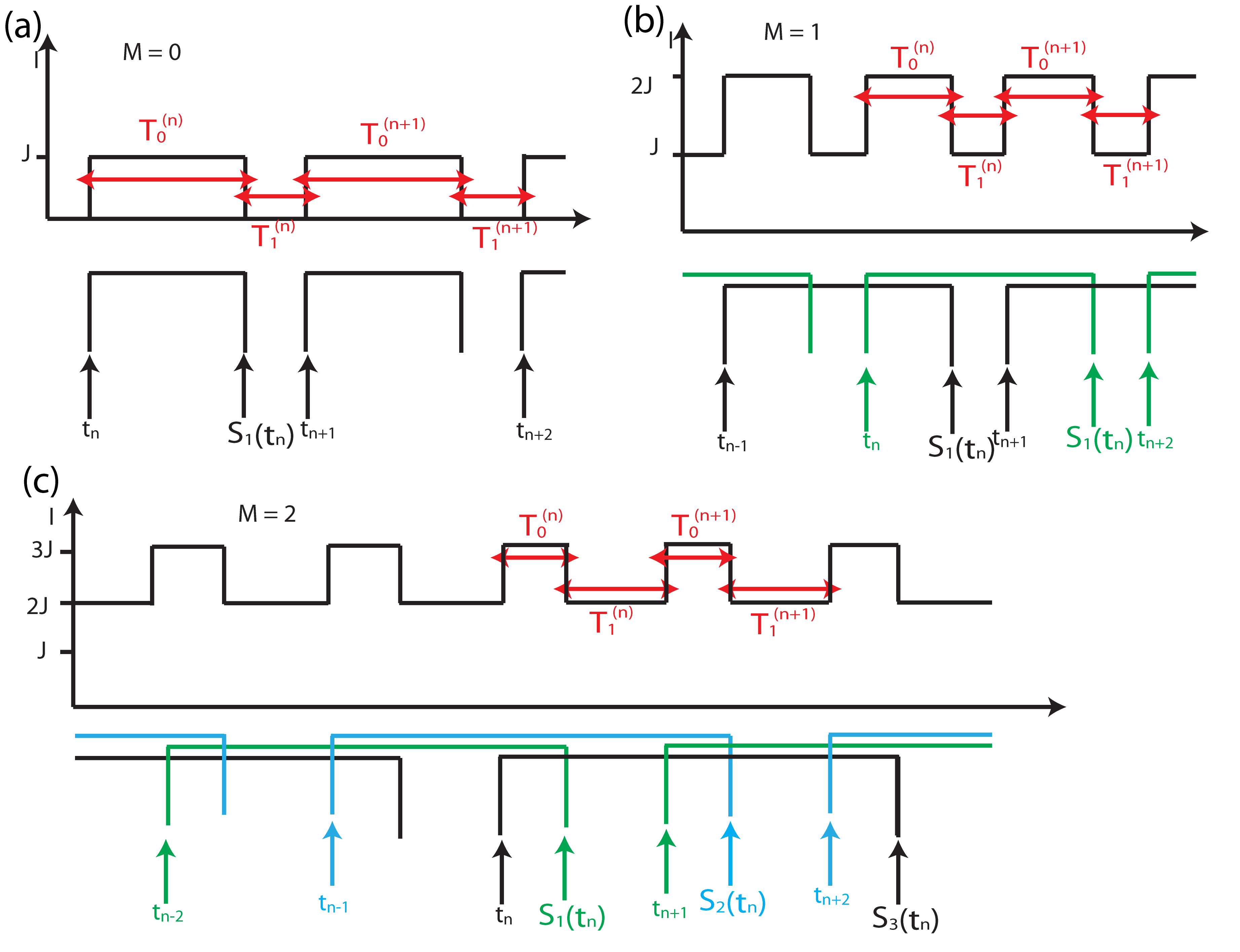
Fig. 1: PSPs in a splay state can overlap $M$ times. (a) PSPs overlapping $M=0$ times (no overlaps); (b) PSPs overlapping $M=1$ times; (c) PSPs overlapping $M=2$ times. Independently of the value of $M$ the synaptic current can take only two values in the time interval between two spikes: namely, during $I(t_{n}<t<t_{n}+T_{0}^{(n)})=(M+1)J$ and $I(t_{n}+T_{0}^{(n)}<t<t_{n+1})=MJ$.

For the splay state we can rewrite the dynamics of each neuron $i$ between two successive spikes occurring at $t_{n}$ and $t_{n+1}$ as an exact map made of the following three steps.

1. The first step starts with a PE at time $t_{n}$, one can easily estimate the evolution of the membrane potential from time $t_{n}^{+}$ to $T_{1}$ when a PT will occur. Let us first define $x_{i}^{(n)}=v_{i}(t_{n}^{+})$ and $y_{i}^{(n)}=v_{i}(t_{n}^{+}+T_{0})$, and order the membrane potentials as follows

   $$x^{(n)}_{1}>x^{(n)}_{2}>...>x^{(n)}_{N}=-\infty\qquad,$$ (18)

   the last equivalence stems from the fact that a neuron has just fired and it has been reset. By employing the expression (7) one gets the following map

   $$y_{i}^{(n)}=\left\{\begin{array}[]{l r}F_{1}(x_{i}^{(n)},T_{0})=H(x^{(n)}_{i},M+1,T_{0}),&i\neq N\\ &\\ F^{*}_{1}(T_{0})=H^{*}(M+1,T_{0}),&i=N\end{array}\right.$$ (19)

   with $H$ and $H^{*}$ defined in (8).

2. The second step corresponds to the integration of the equation of motion from the PT occurring at $t_{n}+T_{0}$ and the time $t_{n+1}^{-}$ immediately preceding the $n+1$-th spike emission. By defining $z_{i}^{(n)}=v_{i}(t_{n+1}^{-})$ and by employing equation (11) one gets

   $$z^{(n)}_{i}=H(y^{(n)}_{i},M,T_{1})$$ (20)

   with $H$ defined in (8). Due to the previous ordering, the next firing neuron will have the label $1$, therefore $z^{(n)}_{1}=\infty$ and thus the denominator of the right side equation (20) should be zero:

   $$1-\beta_{M}(T_{1})y_{1}^{(n)}=0$$ (21)

   By inserting (21) in (20) one gets:

   $$z^{(n)}_{i}=F_{2}(y^{(n)}_{1},y^{(n)}_{i})=\frac{(MJ-1)+y^{(n)}_{1}y^{(n)}_{i}}{y^{(n)}_{1}-y^{(n)}_{i}}$$ (22)

3. The last step amounts simply to calculating the membrane potential change in going from $t_{n+1}^{-}$ to $t_{n+1}^{+}$ and introducing a co-moving frame to maintain the order among the membrane potentials also after each firing event. This amounts to writing

   $$x^{(n+1)}_{i}=F_{3}(z^{(n)}_{i+1})=z^{(n)}_{i+1}\qquad{\rm for}\enskip 1\leq i\leq N-1$$ (23)

   and setting $x_{N}^{(n+1)}=-\infty$. Since the event-driven map approach corresponds to a suitable Poincaré section, we are left with $N-1$ variables, dropping the variable $i=N$.

We can compute the complete event-driven map from spike time $t_{n}$ to spike time $t_{n+1}$, by combining the three above equations (19), (20) and (23)

$$x^{(n+1)}_{i}=F(x^{(n)}_{i+1})=\frac{a_{0}+a_{1}x^{(n)}_{i+1}}{a_{2}+a_{3}x^{(n)}_{i+1}}\qquad{\rm for}\enskip 1\leq i\leq N-1\quad;$$ (24)

where the coefficients entering in (24) reads as:

$$\begin{array}[]{l}a_{0}=(MJ-1)\beta_{M}(T_{1})+[(M+1)J-1]\beta_{M+1}(T_{0})\\ a_{1}=1-(MJ-1)\beta_{M+1}(T_{0})\beta_{M}(T_{1})\\ a_{2}=1-[(M+1)J-1]\beta_{M+1}(T_{0})\beta_{M}(T_{1})\\ a_{3}=-\beta_{M+1}(T_{0})-\beta_{M}(T_{1})\end{array}$$ (25)

Exact firing rate value.

In order to obtain the membrane potential values associated with the splay state one should impose that the splay state represents a fixed point for the event-driven map in the comoving frame, namely

$$x_{i}^{(n)}=x_{i}^{(n+1)}=\tilde{x}_{i}\qquad$$ (26)

Furthermore, once fixed $G$, $N$, and $T_{s}$, one can determine the NISI $T$ by solving iteratively equation (12) together with the set of equations for the membrane potential (24), with the requirement that $x^{*}=F^{N}(\tilde{x}_{N}=-\infty)=+\infty$. Numerically, as a first guess for $T$ we usually employ the mean-field result $1/\nu_{1}$, given by the larger solution of (5). Then we evaluate the splay state by employing a bisection method to find the exact NISI. We stop the procedure whenever $x^{*}>10^{8}$, with the constraint that the order (18) is maintained.

For a given set of parameters $G$, $T_{s}$ and $N$ we found at maximum two coexisting splay states (in agreement with the mean-field results). Beyond a minimal value of $J$, there is always one marginally stable splay state. When the splay states are two we found that the other one is unstable, as illustrated in the following in Fig. 6. Let us stress that unstable branches of solutions exist only for non overlapping pulses (i.e. $M=0$) as shown in Fig. 2. These numerical results will be confirmed by analytical analysis in §A for $N=2,3,4$ and $J<J_{1}$ ($M=0$).

Notice that for $N=2$ only the marginally stable branch exists and the minimal firing rate reaches the value $\nu=0$. Instead for $N>2$ the minimal firing rate of the marginally stable branch is $\nu\neq 0$. The firing rates associated to the unstable branch, for finite $N$, reaches always the value $\nu=0$ for some finite pulse amplitude $J=J^{*}$. Finally, for $N\to\infty$ we have that $J^{*}(\nu=0)\rightarrow\infty$.

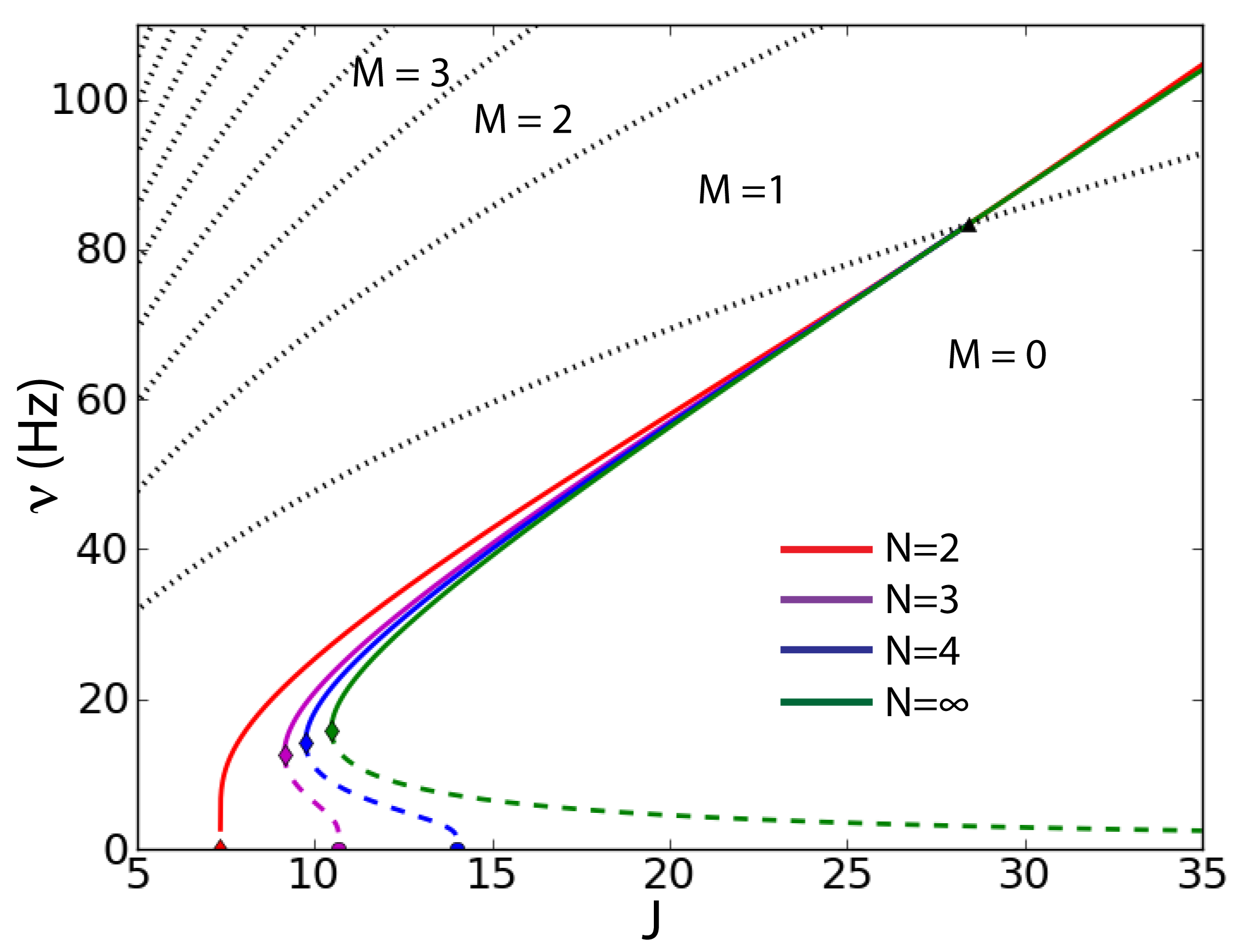
Fig. 2: Frequencies of the splay states as a function of the synaptic strength $J$ and for pulse duration $T_{s}N=12$ ms with $\tau=20$ ms. Red line: $N=2$, magenta line: $N=3$, blue line: $N=4$, green line: $N=\infty$. Black dotted lines separate regions with different number $M$ of overlapping PSPs. Solid lines refer to the upper stable branches of the splay state. Dashed lines refers to the lower unstable branches of the splay state. For $N=2$ the lower branch does not exist.

3.2 $\delta$-pulses

In the case of $\delta$-pulses, the formulation of the event-driven map is extremely simplified, since now there are only PE events. At the arrival of a $\delta$-pulse, we can integrate eq. (1) with the current given by (3) between time $t^{-}_{n}$ and $t^{+}_{n}$, obtaining

$$y^{(n)}_{i}=x^{(n)}_{i}+J_{\delta}\qquad{\rm for}\enskip 1\leq i\leq N-1\quad,$$ (27)

where $J_{\delta}=G/(N\tau)$. The evolution of the membrane potential in the time interval $t_{n}^{+}$ and $t_{n+1}^{-}$ can be easily obtained since it corresponds to eq. (11) with $M=0$ and $T_{1}=t_{n+1}^{-}-t_{n}^{+}=T$, namely

$$z_{i}^{(n)}=H(y^{(n)}_{i},0,T)$$ (28)

for $i=1,\dots,N-1$. Then we can combine eq. (27) and (28) with the change of reference frame (23) to obtain the corresponding event-driven map. The resulting map is identical to that found for the step function (24), apart the value of the coefficients (25) that now become:

$$\begin{array}[]{l}a_{0}=-\beta_{0}(T)+J_{\delta}\\ a_{1}=1\\ a_{2}=1-\beta_{0}(T)J_{\delta}\\ a_{3}=-\beta_{0}(T)\end{array}$$ (29)

Once fixed $J_{\delta}$ and $N$ and $T_{s}$, similarly to the case of step pulses, one can determine $T$ together with the membrane potential values associated with the splay state by solving iteratively equation (12), and by applying iteratively the map (24) with coefficients (29) starting from $\tilde{x}_{N}=-\infty$. The solution is numerically achieved whenever $x^{*}=F^{N}(\tilde{x}_{N}=-\infty)=+\infty$ (namely, $x^{*}>10^{8}$) and the condition (18) is satisfied.

We want to conclude this Section by mentioning the fact that in the limit $N\to\infty$ we were able to derive an explicit analytic expression for the membrane potentials corresponding to a splay state. The detailed calculations are reported in §B.

4 Linear Stability Analysis for Step Pulses

We are interested in the linear stability of the splay state in the case of step pulses for finite system size $N$. It is therefore useful to introduce the following vector notation for the membrane potentials at spike time $t_{n}$:

$$\mathbf{x}^{(n)}=\left\{x^{(n)}_{1},x^{(n)}_{2},\cdots,x^{(n)}_{N}\right\}\qquad;$$ (30)

Furthermore, if we have more than one overlapping pulse, i.e. if $M>0$, the actual state of the network will depend not only on the membrane potential values but also on the past $M$ spike times $\{t_{k}\}$ with $k=n-M,n-M+1,\dots,n-1$. However the formulation of the tangent space dynamics can be made simpler by introducing the related time intervals $\tau^{(n)}_{j}\equiv t_{n}-t_{n-j}$:

$$\mathbf{\tau}^{(n)}=\left\{\tau^{(n)}_{1},\tau^{(n)}_{2},\cdots,\tau^{(n)}_{M}\right\}$$ (31)

In this notation the splay state is a fixed point of the network dynamics satisfying the following relationships:

$$\tilde{\mathbf{x}}=F_{3}(\tilde{\mathbf{z}})=F_{3}(F_{2}(\tilde{\mathbf{y}}))=F_{3}(F_{2}(F_{1}(\tilde{\mathbf{x}})))\quad,$$ (32)

and

$${\tilde{\tau}}_{j}=j\cdot T\qquad j=1,\dots,M\qquad.$$ (33)

4.1 Linearized Poincaré map

In order to derive the equations of evolution in the tangent space for our case it is convenient to consider separately the three steps in eq. (32), please notice that now $T_{0}^{(n)}$ and $T_{1}^{(n)}$ depend on the spike sequence index $n$ since, for the perturbed dynamics these quantities are no more constant.

Let us start by perturbing eq. (19):

$$\left\{\begin{array}[]{l l}\delta y^{(n)}_{i=1,...,N-1}&=d_{i}\delta x_{i}^{(n)}+s_{i}\delta T^{(n)}_{0}\\ &\\ \delta y^{(n)}_{N}&=s_{N}\delta T^{(n)}_{0}\end{array}\right.$$ (34)

with $\delta T^{(n)}_{0}=0$ if $M=0$; where the coefficients are:

$$d_{i}=\left.\frac{\partial F_{1}(x^{(n)}_{i},T^{(n)}_{0})}{\partial x^{(n)}_{i}}\right|_{\tilde{x}_{i},\tilde{T}_{0}}=\frac{1+[(M+1)J-1]\beta^{2}_{M+1}(\tilde{T}_{0})}{(1-\beta_{M+1}(\tilde{T}_{0})\tilde{x}_{i})^{2}}\qquad,$$ (35)

$$s_{i}=\left.\frac{\partial F_{1}(x^{(n)}_{i},T^{(n)}_{0})}{\partial T^{(n)}_{0}}\right|_{\tilde{x}_{i},\tilde{T}_{0}}=\frac{(M+1)J-1+\tilde{x}^{2}_{i}}{(1-\beta_{M+1}(\tilde{T}_{0})\tilde{x}_{i})^{2}}\frac{1}{\cos^{2}\left(\sqrt{(m+1)g-1}\tilde{T}_{0}/\tau\right)}\frac{1}{\tau}\qquad,$$ (36)

$$s_{N}=\left.\frac{dF^{*}_{1}(T^{(n)}_{0})}{dT^{(n)}_{0}}\right|_{\tilde{T}_{0}}=\frac{1}{\beta^{2}_{M+1}(\tilde{T}_{0})}\frac{1}{\cos^{2}\left(\sqrt{(M+1)J-1}\tilde{T}_{0}/\tau\right)}\frac{1}{\tau}\qquad;$$ (37)

As a second step we perturb $F_{2}$ given by eq. (22), obtaining

$$\delta z^{(n)}_{i}=h_{i}\delta y^{(n)}_{1}+k_{i}\delta y^{(n)}_{i}\qquad i=1,\dots,N\quad;$$ (38)

remember that if $M=0$ then $\delta y^{(n)}_{N}=0$. The coefficient $h_{i}$ and $k_{i}$ are defined as:

$$h_{i}=\left.\frac{\partial F_{2}(y^{(n)}_{1},y^{(n)}_{i})}{\partial y^{(n)}_{1}}\right|_{\tilde{y}_{1},\tilde{y}_{i}}=-\frac{MJ-1+\tilde{y}^{2}_{i}}{(\tilde{y}_{1}-\tilde{y}_{i})^{2}}\qquad,$$ (39)

$$k_{i}=\left.\frac{\partial F_{2}(y^{(n)}_{1},y^{(n)}_{i})}{\partial y^{(n)}_{i}}\right|_{\tilde{y}_{1},\tilde{y}_{i}}=\frac{MJ-1+\tilde{y}^{2}_{1}}{(\tilde{y}_{1}-\tilde{y}_{i})^{2}}\qquad.$$ (40)

Finally, the linearized equations associated with the reference frame change can be obtained by perturbing eq. (23):

$$\delta x_{i}^{(n+1)}=\delta z_{i+1}^{(n)}\qquad i=1,\dots,N-1\qquad,$$ (41)

please notice that $\delta x_{N}^{(n)}\equiv 0$ due to the fact that in the comoving frame $x_{N}^{(n)}\equiv-\infty$, therefore the evolution in the tangent space should deal with only $N-1$ perturbations associated to the membrane potentials.

Then we need to compute how the time interval $T^{(n)}_{0}$ is modified by the perturbations, when $M>0$. The key point here is that $T^{(n)}_{0}$ depends on the previous spike times as follows:

$$T^{(n)}_{0}=T_{s}-(t_{n}-t_{n-M})=T_{s}-\tau_{M}^{(n)}\qquad;$$ (42)

apparently one could be lead to think that we need only an extra variable: $\tau^{(n)}_{M}$. However, $\tau^{(n)}_{M}$ depends on all the $M$ previous spike times and therefore we need to take in account also the perturbations of the other $M-1$ variables, namely $\tau^{(n)}_{j=1,...,M-1}$.

To obtain the evolution equations for these auxiliary $M$ variables, let us consider the following relations

$$\tau^{(n+1)}_{1}=T^{(n)}_{0}+T^{(n)}_{1}$$ (43)

and

$$\tau^{(n+1)}_{j}=\tau^{(n+1)}_{1}+\tau^{(n)}_{j-1}=T^{(n)}_{0}+T^{(n)}_{1}+\tau^{(n)}_{j-1}\quad.$$ (44)

From (42) we obtain the relation $\delta\tau^{(n)}_{M}=-\delta T^{(n)}_{0}$. From this relation and from equations (43) and (44) (for positive $M$) we can easily obtain the evolution maps for the perturbed quantities:

$$\left\{\begin{array}[]{l l}\delta\tau^{(n+1)}_{1}&=\delta T^{(n)}_{1}-\delta\tau^{(n)}_{M}\\ &\\ \delta\tau^{(n+1)}_{j=2,...,M}&=\delta T^{(n)}_{1}+\delta\tau^{(n)}_{j-1}-\delta\tau^{(n)}_{M}\end{array}\right.$$ (45)

We are left just with the determination of $\delta T^{(n)}_{1}$, this can be derived by remembering that the time from the last PT until the next PE can be calculated by employing eq. (12) with $K=M$, $v_{p}(t^{+}-n)$, and $E(t^{*})-t^{*}=T^{(n)}_{1}$:

$$T^{(n)}_{1}=G(y^{(n)}_{1})=\left\{\begin{array}[]{l l}MJ<1&\frac{\tau}{\sqrt{MJ-1}}\tanh^{-1}\left(\frac{\sqrt{MJ-1}}{y^{(n)}_{1}}\right)\\ \\ MJ>1&\frac{\tau}{\sqrt{MJ-1}}\tan^{-1}\left(\frac{\sqrt{MJ-1}}{y^{(n)}_{1}}\right)\\ \end{array}\right.$$ (46)

and

$$w=\left.\frac{dG}{dy^{(n)}_{1}}\right|_{\tilde{y}_{1}}=-\frac{\tau}{\tilde{y}^{2}_{1}+|MJ-1|}\qquad;$$ (47)

and we can obtain:

$$\delta T^{(n)}_{1}=w\delta y^{(n)}_{1}\qquad.$$ (48)

By combining eq. (34), (38), (41), (45), and (48), the complete map evolution in the tangent space can be finally written as follows:

$$\left\{\begin{array}[]{l l}\delta x_{i=1,...,N-2}^{(n+1)}&=p_{i+1}\delta x_{1}^{(n)}+q_{i+1}\delta x_{i+1}^{(n)}+u_{i+1}\delta\tau^{(n)}_{M}\\ &\\ \delta x_{N-1}^{(n+1)}&=p_{N}\delta x_{1}^{(n)}+u_{N}\delta\tau^{(n)}_{M}\\ &\\ \delta\tau^{(n+1)}_{1}&=r_{1}\delta x_{1}^{(n)}+r_{2}\delta\tau^{(n)}_{M}\\ &\\ \delta\tau^{(n+1)}_{j=2,...,M}&=r_{1}\delta x_{1}^{(n)}+\delta\tau^{(n)}_{j-1}+r_{2}\delta\tau^{(n)}_{M}\end{array}\right.$$ (49)

where we have set $p_{i}=h_{i}d_{1}$, $q_{i}=k_{i}d_{i}$, $u_{i}=-(h_{i}s_{1}+k_{i}s_{i})$, $r_{1}=wd_{1}$, and $r_{2}=-(1+ws_{1})$.

In order to determine the stability of the splay state we should compute the Floquet spectrum by setting

$$\left(\begin{array}[]{c}\delta x^{(n+1)}_{1}\\ ...\\ \delta x^{(n+1)}_{N-1}\\ \delta\tau^{(n+1)}_{1}\\ \vdots\\ \delta\tau^{(n+1)}_{M}\end{array}\right)=\mu_{l}\left(\begin{array}[]{c}\delta x^{(n)}_{1}\\ ...\\ \delta x^{(n)}_{N-1}\\ \delta\tau^{(n)}_{1}\\ \vdots\\ \delta\tau^{(n)}_{M}\end{array}\right)$$ (50)

where $\mu_{l}={\rm e}^{\lambda_{l}+i\omega_{l}}$ ($l=1,\dots,N+M-1$) are the so called (complex) Floquet multipliers, while $\lambda_{l}$ (resp. $\omega_{l}$) are real numbers termed Floquet exponents (resp. frequencies). If $||\mu_{l}||<1$ $\forall l$ (resp. $||\mu_{k}||>1$ for at least one $k$) the splay state is stable (resp. unstable). Whenever the largest modulus of the Floquet multipliers is exactly one the system is marginally stable.

The Floquet spectrum can be obtained by solving the following characteristic polynomial, obtained from eq. (49):

$$\begin{array}[]{c}\left(\mu^{N-1}_{l}-p_{2}\mu^{N-2}_{l}-\sum^{N}_{k=3}p_{k}\left(\prod^{k-1}_{j=2}q_{j}\right)\mu^{N-k}_{l}\right)\left(\mu^{M}_{l}-r_{2}\sum^{M-1}_{k=0}\mu^{k}_{l}\right)+\\ \\ +\left(u_{2}\mu^{N-2}_{l}+\sum^{N}_{k=3}u_{k}\left(\prod^{k-1}_{j=2}q_{j}\right)\mu^{N-k}_{l}\right)\left(-r_{1}\sum^{M-1}_{k=0}\mu^{k}_{l}\right)=0\qquad,\end{array}$$ (51)

which admits $N+M-1$ solutions.

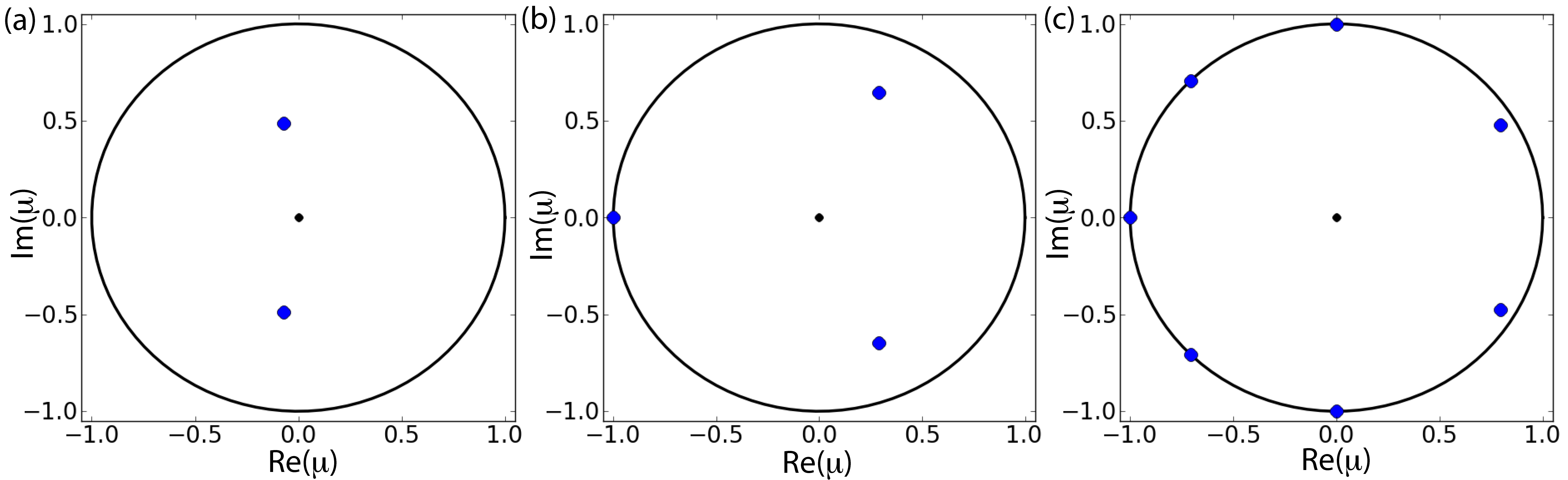
Fig. 3: Floquet multipliers $\{\mu_{l}\}$ for the case with no overlap, i.e $M=0$: (a) $N=3$, $0$ marginally stable eigenvalue; (b) $N=4$, $1$ marginally stable eigenvalue; (c) $N=8$, $5$ marginally stable eigenvalues. In this case we fixed $J=15$ and $NT_{s}=16$ ms and we vary the network size.

4.2 Floquet multipliers

As stated by Watanabe and Strogatz (WS) [29] for a network on $N$ fully coupled phase oscillators with sinusoidal coupling, the system has in general $N-3$ marginally stable directions, furthermore for a splay state, which is a periodic solution, these directions reduce to $N-2$. Therefore since also our model, as detailed in §C, satisfies the hypothesis for which the WS results apply, and since in the event-driven map formulation one degree of freedom is lost, we expect that for the splay states at least $N-3$ Floquet multipliers lie on the unit circle, as shown in Fig. 3 for $M=0$. Furthermore, in presence of overlaps, i.e. for $M>0$, the Floquet exponents associated to the auxiliary variables ${\bf\tau}^{(n)}$ do not influence the stability of the splay state, since these additional $M$ exponents are located within the unit circle, and therefore associated to stable directions as shown in Fig. 4 and 5.

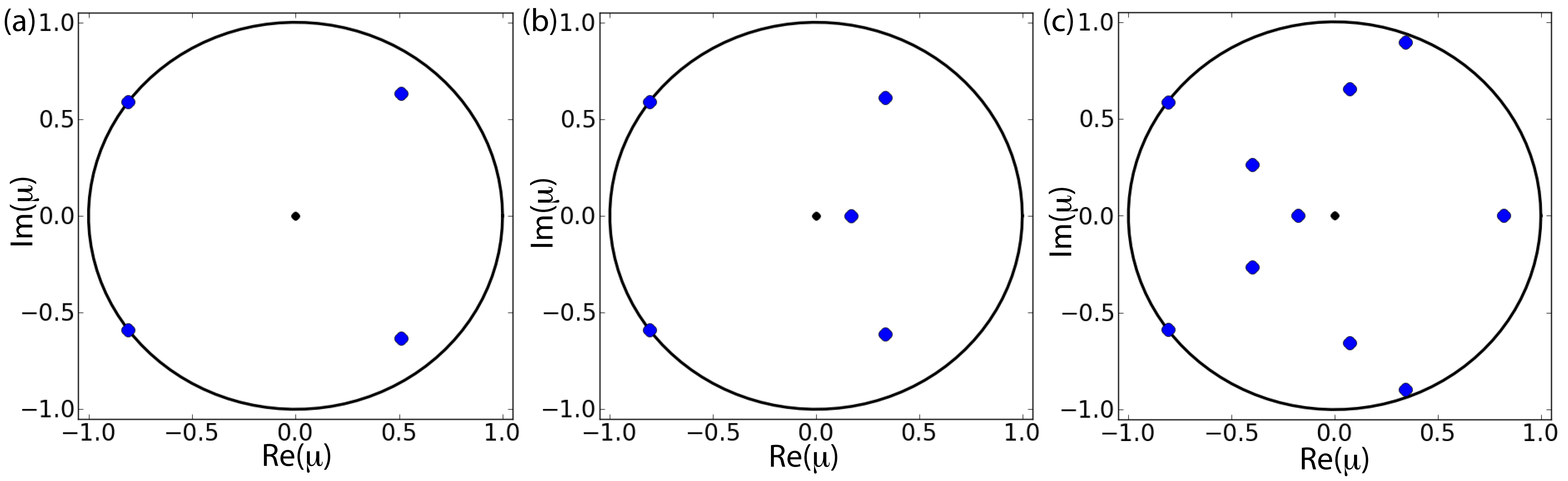
Fig. 4: Floquet multipliers $\{\mu_{l}\}$ for overlapping pulses, i.e. $M>0$ : (a) $J=15$, $M=0$, $2$ neutrally stable eigenvalues; (b) $J=25$, $M=1$, $2$ neutrally stable eigenvalues; (c) $J=100$, $M=6$, $2$ neutrally stable eigenvalues. We have considered $N=5$ and $T_{s}=3.2$ ms.

It is interesting to notice how the additional exponents associated to the auxiliary variables emerge by increasing the number of overlaps. In particular, the number of overlaps can be increased from $M$ to $M+1$ by varying the coupling $J$ from below to above the threshold $J_{M+1}$. At the threshold $J_{M+1}$ a new variable $\tau_{M+1}$ is added to the event-driven map describing the system. Therefore the Floquet spectrum associated with the corresponding splay state solution has one additional eigenvalue. This new direction emerges as superstable at $J=J_{M+1}$ being associated to a zero Floquet multiplier, as shown in Fig. 5. By further increasing $J$ the new eigenvalue increases its modulus, which however remains always smaller than one.

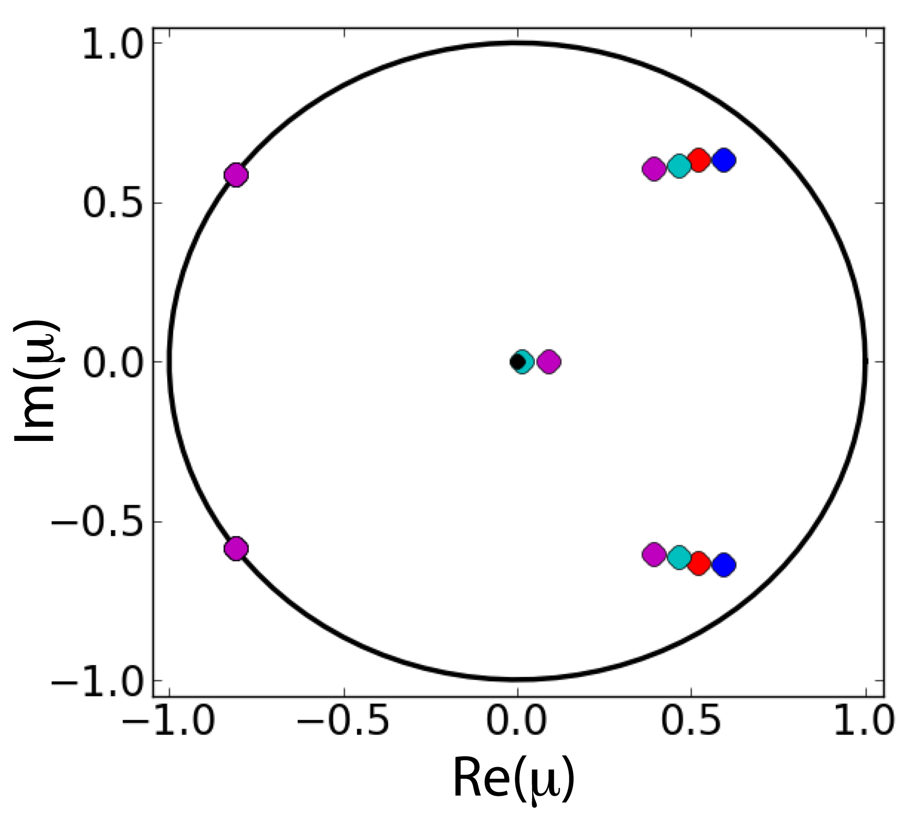
Fig. 5: (a) Floquet spectrum of the splay state in the complex plane for $T_{s}N=16$ ms, $N=5$, in this case $J_{1}=16.42$. Blue stars correspond to $M=0$ when $J=10.42<J_{1}$ (blue), and $J=14.42<J_{1}$ (red); and to $M=1$ when $J=18.42>J_{1}$ (cyan), and $J=22.42>J_{1}$ (magenta)

In Fig. 6 we report the Floquet multipliers associated to the unstable branch of splay state solutions, which coexist with the marginally stable branch for $N>2$, as already mentioned in Sect. III A.

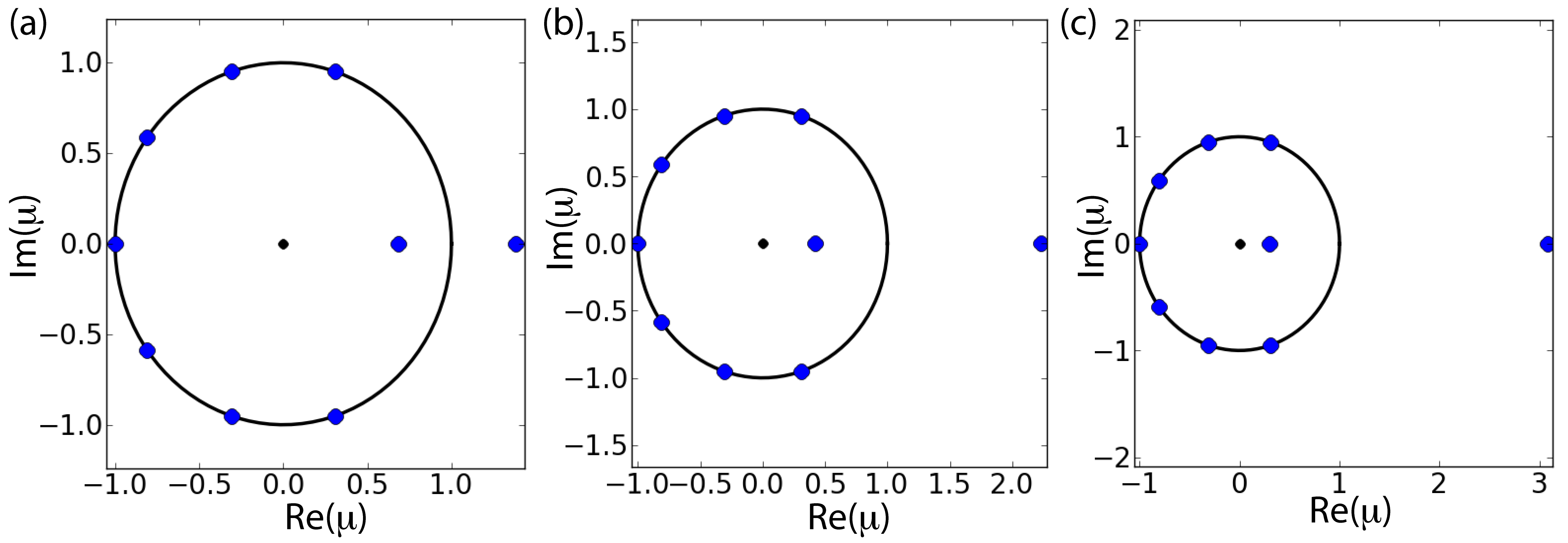
Fig. 6: Floquet spectrum of the splay state in the complex plane for the unstable branch, $T_{s}N=16$ ms, $N=10$: (a) $J=8$, (b) $J=10$, (c) $J=12$.

5 Linear Stability for $\delta$-pulses

In the case of $\delta$-pulses the stability of the splay state can be inferred by theoretical arguments based on the symmetry of the considered model and of the specific pulse coupling. It is evident that the QIF model (1) for time symmetric pulses has a time reversal symmetry. This can be appreciated as follows. Given a solution $\mathbf{v}(t)=\{v_{1}(t),\ldots,v_{N}(t)\}$ we define $\mathbf{w}(t)=\{w_{1}(t),\ldots,w_{N}(t)\}=-\{v_{N}(-t),\ldots,v_{1}(-t)\}$. It is clear from the time reversal property of (1) that $\mathbf{w}(t)$ is a solution in between two spike emissions. Let us analyze if the symmetry is maintained also during spike emission, in the usual case $v_{1}$ will reach $\infty$, then it will be reset to $-\infty$ and a constant value $J_{\delta}$ will be added to all the other membrane potentials. The membrane potential $w_{1}(t)$ reaching $\infty$ is equivalent to $v_{N}(-t)$ reaching $-\infty$. Backwards in time the reset and coupling consists of setting $v_{N}$ to $\infty$ and subtracting $J_{\delta}$ from the other variables. Due to the minus sign in the definition of $\mathbf{w}(t)$ this means that $w_{1}$ is reset from $+\infty$ to $-\infty$ and the other variables are incremented by $J_{\delta}$. Hence $\mathbf{w}(t)$ is a solution and (1) has time reversal symmetry.

We also show that the splay state is transformed to itself by the time reversal. A splay state is a solution $\mathbf{v}(t)$ characterized by the following properties

$$v_{j}(t+T)=v_{j+1}(t),\qquad v_{j}(t+NT)=v_{j}(t)\qquad j=1,\ldots,N.$$ (52)

Note that if $\mathbf{w}(t)$ is the time reversal of $\mathbf{v}(t)$ then $w_{j}(t)=-v_{N-j+1}(-t)$, $j=1,\ldots,N$. We now make the following computation:

$$\begin{split}w_{j}(t+T)&=-v_{N-j+1}(-t-T)\\ &=-v_{N-j}(-t-T+T)\\ &=-v_{N-(j+1)-1}(-t)=w_{j+1}(t)\quad.\end{split}$$ (53)

It follows that $\mathbf{w}(t)$ is also a splay state. Moreover, by choosing the phase, we can set $v_{1}(0)=0$, which implies that $v_{1}(0)=w_{N}(0)$, or $v_{1}(0)=w_{1}((N-1)T)$. Therefore $\mathbf{w}(t)$ must be a phase shifted version of $\mathbf{v}(t)$.

We now use the following well known result [21]:

Theorem 1.

Let

$$\dot{\mathbf{x}}=F(\mathbf{x}),\qquad\mathbf{x}\in{\cal R}^{N}$$ (54)

be an ordinary differential equation and $R$ a matrix. Suppose that (54) has a time reversal symmetry defined as follows: if $\mathbf{x}(t)$ is a solution of (54) then $\mathbf{y}(t)=-R\mathbf{x}(-t)$ is also a solution. Suppose also that (54) has a periodic solution $\mathbf{x}_{0}(t)$ such that $-R\mathbf{x}_{0}(-t)=\mathbf{x}_{0}(t+T)$, for some $T$. Then all the Floquet multipliers of $\mathbf{x}_{0}(t)$ are on the unit circle.

It follows from Theorem 1 that the splay phase solution has all its Floquet multipliers on the unit circle (as shown in Fig. 7). In particular, in Fig. 7 we report the Floquet multipliers for two different shape of PSP, but maintaining the the same coupling weight $G$, we observe that the multipliers which were inside the unit circle attain modulus one by passing continuously from step to $\delta$-pulses.

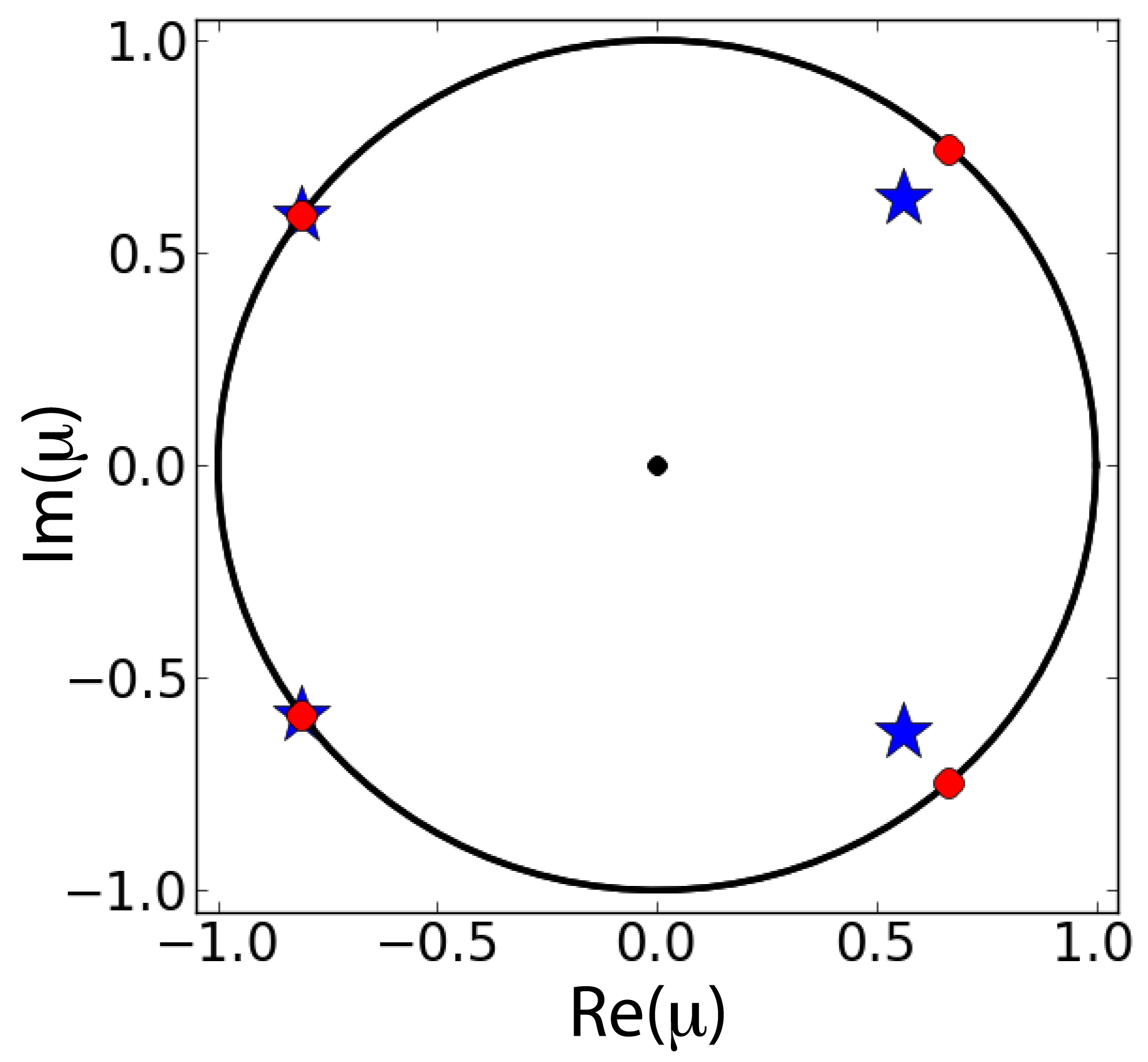
Fig. 7: Floquet multipliers for splay state with different PSPs: namely, blue stars refer to step functions with $J=10$, and red circles to $\delta$-functions. The coupling weight is the same in the two cases, $G=180$ ms.

6 Continuous Family of Periodic Solutions

We want to show that the $N-3$ directions of neutral stability for the splay state are not only local but also global. We have verified this issue numerically, by perturbing randomly the splay state $\tilde{\mathbf{x}}$ and by following the system dynamics, with the aid of the general event-driven map discussed in §3A, until its convergence to some stationary state. In particular, the initial conditions for these simulations have been generated as follows

$$\mathbf{x}=\tilde{\mathbf{x}}+\sigma\mathbf{\mathcal{N}}\qquad,$$ (55)

where $\tilde{\mathbf{x}}$ identifies the splay state, $\mathcal{N}$ is a $N$-dimensional random vector whose components are $\delta$-correlated with zero average and Gaussian distributed with unitary standard deviation, and the noise amplitude is $\sigma=0.1$. By following the time evolution for a sufficiently long time span (typically, of order of $100\cdot N$ spikes), we always observe that these initial conditions converge to periodic orbits or to the quiescent state $\mathbf{x}=\{-1,...,-1\}$. This has been verified for system size up to $N=1,000$ and by considering up to $10,000$ different initial conditions for each $N$.

Furthermore we observe that the final state is an orbit with periodicity $\chi=N$ if $N>4$ and periodicity $\chi=2$ if $N=4$ (Fig. 8). For $N=3$ the final state is always the splay state. These solutions are characterized by neurons firing periodically with the same period, but with time intervals among successive firing which are not constant, like for the splay state. Please notice that, in the event-driven map context, the splay state amounts to a fixed point of the dynamics.

All the the periodic orbits we found lie on the $(N-3)$-manifold associated to the neutrally stable directions of the splay state in the event-driven map formulation, that can be obtained by eq. (49). We can affirm this, since on one hand we have verified that by perturbing the splay state along the stable directions we end up to the splay state itself (as shown in Fig. 8(a)), while while by perturbing along the neutrally stable directions we always end up in one of these many periodic orbits (as shown in Fig. 8(b)). On the other hand, by perturbing one of these orbits along the stable directions of the splay state the perturbed system converges to the same orbit (see Fig. 8(c)), while by perturbing along the neutrally stable directions the system ends up on a different periodic orbit (see Fig. 8(d)). Therefore these periodic orbits are also neutrally stable and share the same neutrally stable manifold of the splay state.

The existence of this manifold made of a continuous family of periodic solutions has been previously reported for Josephson arrays [27, 13] and Watanabe and Strogatz discussed the generality of this issue, reporting a “heuristic” argument to support the existence of this manifold for generic fully coupled oscillator networks with sinusoidal coupling [29].

As a last point we have evaluated for the splay state and several periodic orbits (namely $N_{t}=10,000$) the single neuron firing rate $\nu$. The distribution of these rates is reported in Fig. 9, revealing that the splay state is characterized by the minimal firing rate with respect to the ones found for the associated family of periodic orbits.

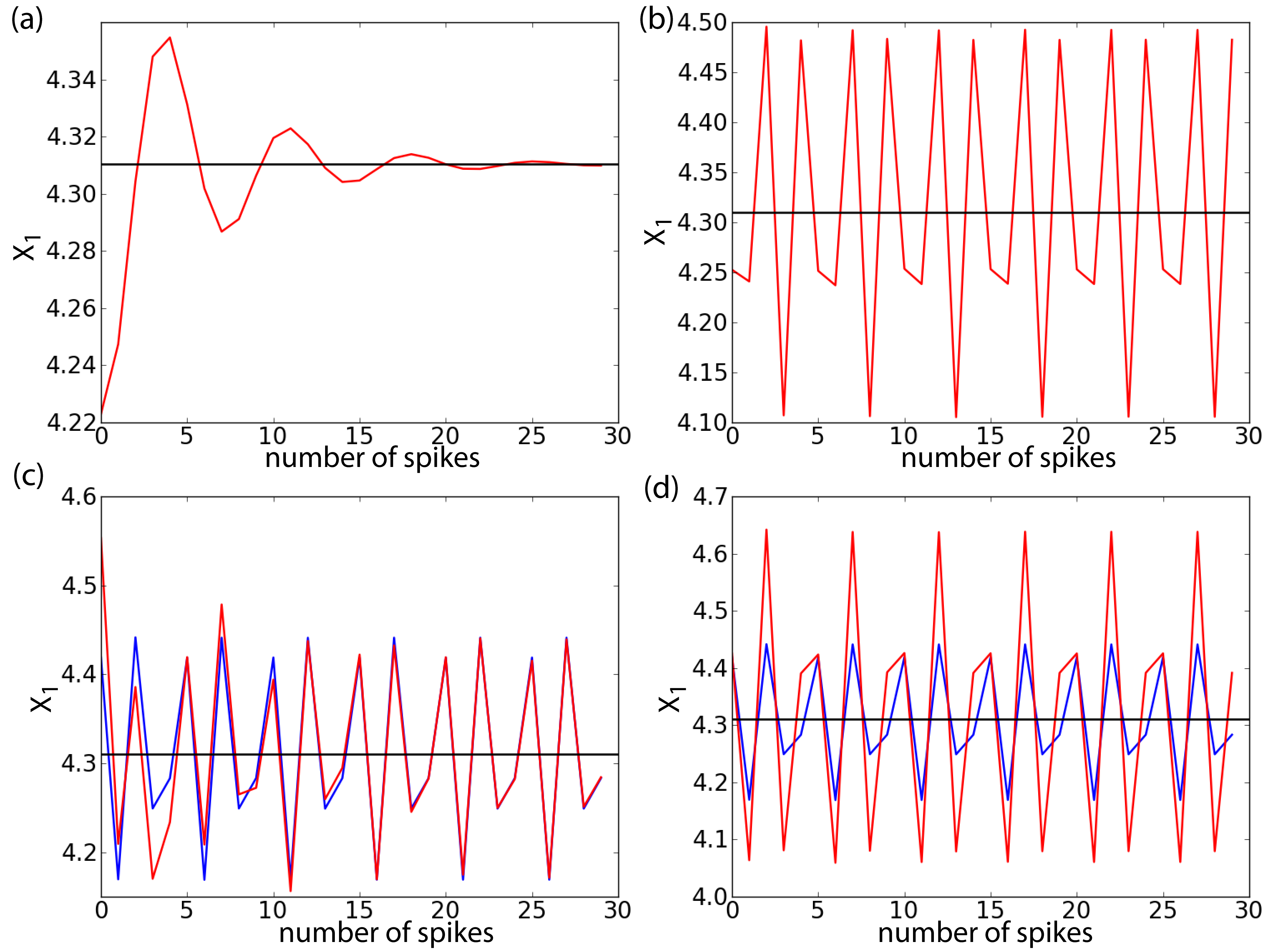
Fig. 8: Examples of trajectories (red lines) emerging from the perturbation of the splay state (black lines) or of a periodic state (blue lines). Only the voltage variable $x_{1}$ is reported here as a function of the index labeling the sequence of successive firings. Perturbation of the splay state: (a) along the directions of stability, the system converges to the splay state; (b) along the directions of neutral stability, the system is set in a periodic state. Perturbation of a periodic state: (c) along the directions of stability, the system converges to the periodic orbit; (d) along the directions of neutral stability, the system is set in a new periodic orbit. The system parameters are $N=5$, $J=15$, and $T_{s}=3$ ms, and $\sigma=0.2$.

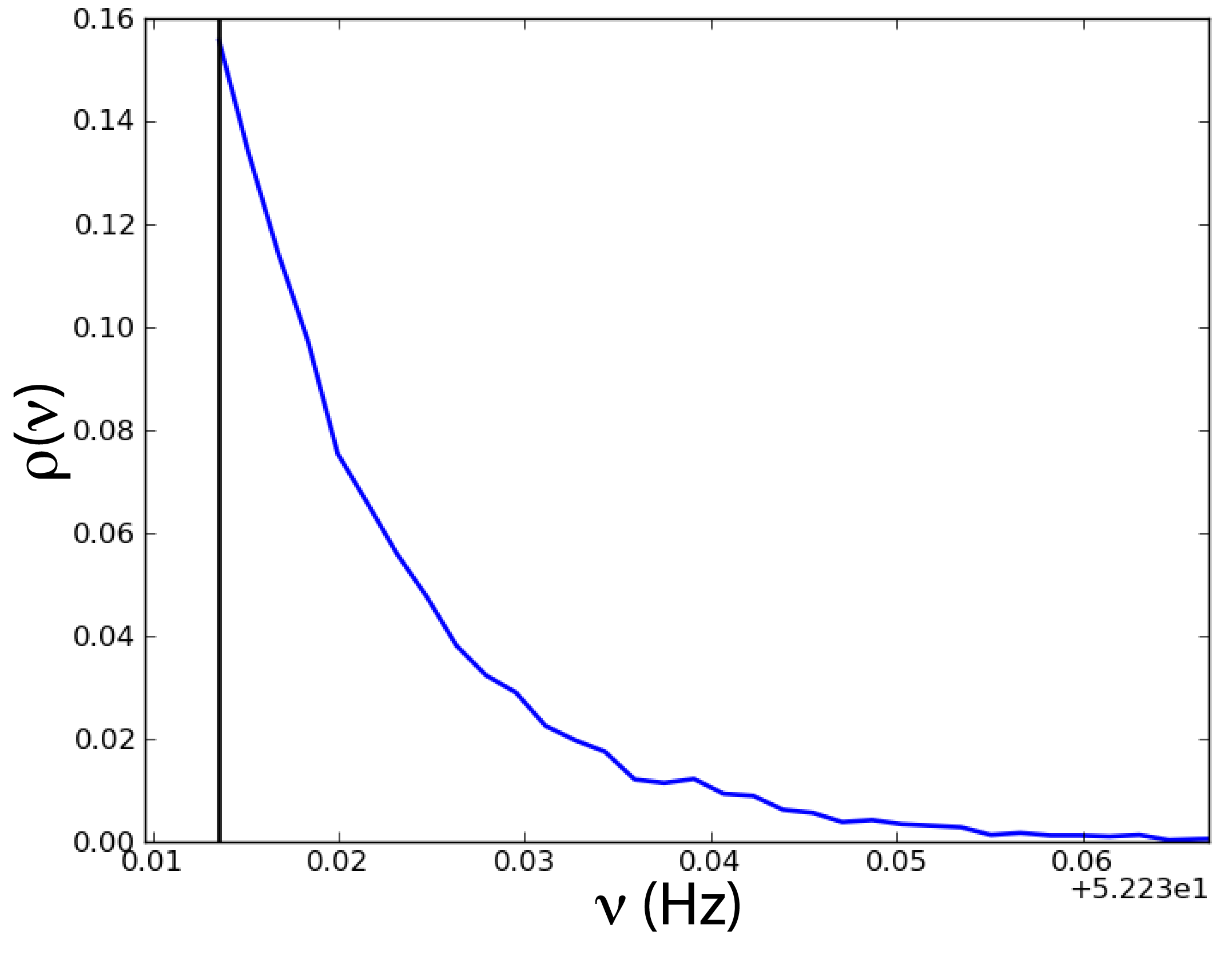
Fig. 9: Probability distribution of the single neuron firing rate $\nu$ for the periodic solutions and the splay state (vertical black line). The $N_{t}$ initial condition are generated by randomly perturbing the splay state along the directions of neutral stability, the perturbations were gaussian distributed with zero average.The model parameter are the same as in the previous figure. and $N_{t}=10,000$.

7 Conclusions

In this paper we showed analytically that finite-size all-to-all pulse-coupled excitatory networks of excitable neurons admit marginally stable persistent splay states. We obtained analytical information about the stable firing rates of these sustained activities. Since the firing rate of persistent states is an electrophysiologically measurable quantity in a working memory tasks, these results can provide insights for working memory models. We further obtained results on the splay state stability that can help in choosing the correct parameters required for biologically relevant working memory models. Our results also give an analytical basis to previous observations in models that the stable sustained neural activity is asynchronous [20, 8].

We developed event-driven map methods to analyze the network dynamics and found an analytical expression for the Floquet spectra associated to the splay state for step pulses and $\delta$-pulses. In the case of $M$ overlapping synaptic step pulses our analysis has revealed that for a correct treatment of the linear stability analysis, the evolution of $M$ additional variables, corresponding to the last $M$ firing events, should be taken in account.

Our analysis, extending previous results for systems with sinusoidal coupling [29], revealed that the splay state is marginally stable for finite size networks with $N-2$ neutral directions, which reduce to $N-3$ in the event-driven map formulation. We also reported a rigorous proof for non overlapping step pulses. We further identified a continuous family of periodic solutions surrounding the splay state. Their peculiarity is that these periodic states have exactly the same neutral stability directions as the splay state.

Our results leave several open questions, in particular we need to proof that at least one of the splay states is Lyapunov stable, when they exist. It would be also of interest to extend the rigorous results reported in §C to overlapping PSPs. Furthermore, since the stable persistently active solutions of our network have a specific spiking structure, splay or families of periodic solutions, it would be interesting to identify the structure of the unstable states that form the separatices between this sustained activity and the ground state. Finally we should explain why all the marginally stable states are periodic.

Appendix A Explicit solution of the splay state firing rate for small network sizes

In this Appendix we will show how it is possible to obtain explicitly the firing rate $\nu$ of the splay state, for $N=2,3,4$, and for $M=0$ (namely for $J<J_{1}$).

A.1 Step pulses

Eq. (20) can be rewritten in the following way

$$y^{(n)}_{i}=\frac{-(1-\gamma)+(1+\gamma)x_{i}^{(n)}}{(1+\gamma)-(1-\gamma)x^{(n)}_{i}}$$ (56)

where we have made use of the variable

$$\gamma=\exp(-2T_{1}/\tau)\qquad;$$ (57)

Since in the present case $0<T_{s}<T$ the values of $\gamma$ are bounded between 0 and 1.

By employing (19), (56), and (23), the coefficients of the event-driven map (24) can be rewritten as

$$\begin{array}[]{l}a_{0}=-(1-\gamma)+(1+\gamma)(J-1)\beta_{1}(T_{s})\\ a_{1}=(1+\gamma)+(1-\gamma)\beta_{1}(T_{s})\\ a_{2}=(1+\gamma)-(1-\gamma)(J-1)\beta_{1}(T_{s})\\ a_{3}=-(1-\gamma)-(1+\gamma)\beta_{1}(T_{s})\end{array}$$ (58)

The firing rate can be obtained in an explicit form by inverting (57), namely

$$\nu=\frac{1}{NT}=\frac{1}{N}\frac{1}{T_{s}-\frac{\tau}{2}\ln\left(\gamma(N,J,T_{s})\right)}$$ (59)

Once fixed the network parameters, an admissible solutions for $\gamma\in[0;1]$ amounts finding a splay state solution with a frequency given by (59).

Given an admissible $\gamma$ value, the membrane potentials corresponding to the splay state can be found by iterating the map (24) starting from the boundary condition $\tilde{x}(N)=-\infty$ corresponding to the reset value, namely

$$\left(\begin{array}[]{c}\tilde{x}_{N-1}\\ \tilde{x}_{N-2}\\ \vdots\\ \tilde{x}_{2}\\ \tilde{x}_{1}\\ \tilde{x}_{0}\\ \end{array}\right)=\left(\begin{array}[]{c}a_{1}/a_{3}\\ (a_{0}a_{3}+a^{2}_{1})/(a_{3}(a_{1}+a_{2}))\\ \vdots\\ -(a_{0}a_{3}+a^{2}_{2})/(a_{3}(a_{1}+a_{2}))\\ -a_{2}/a_{3}\\ \infty\\ \end{array}\right)$$ (60)

We can finally determine $\nu$ analytically for $N=2,3,4$.

• In the case of a couple of neurons, $N=2$, we should impose $\tilde{x}_{1}=\tilde{x}_{N-1}$ and thus we have $a_{1}+a_{2}=0$. Solving this equation for $\gamma$ we obtain:

  $$\gamma=\frac{(J-2)\beta_{1}(T_{s})-2}{(J-2)\beta_{1}(T_{s})+2}$$ (61)

  in this case we have a unique stable branch of solutions, as shown in Fig. 2 Furthermore, the minimal reachable frequency is zero and it is achieved for $\gamma=0$, when $J$ and $T_{s}$ satisfy the equation $(J-2)\beta_{1}(T_{s})=2$.

• For $N=3$ we have $\tilde{x}_{1}=\tilde{x}_{N-1}$, using the values in (60) we obtain:

  $$a_{0}a_{3}+a^{2}_{1}+a^{2}_{2}+a_{1}a_{2}=0$$ (62)

  and then, we can reorder this equation as a second order equation for $\gamma$:

  $$[(J-2)\beta_{1}(T_{s})+2]^{2}\gamma^{2}-2[(J^{2}-2J+2)\beta^{2}_{1}(T_{s})-2]\gamma+[(J-2)\beta_{1}(T_{s})-2]^{2}=0$$ (63)

  this equation admits the following two solutions

  $$\begin{array}[]{l}\gamma_{1,2}=\{[(J^{2}-2J+2)\beta^{2}_{1}(T_{s})-2]\pm\\ \\ \pm\sqrt{[(J^{2}-2J+2)\beta^{2}_{1}(T_{s})-2]^{2}-[(J-2)^{2}\beta^{2}_{1}(T_{s})-4]^{2}}\}\cdot\\ \\ \cdot\{[(J-2)\beta^{2}_{1}(T_{s})+2]^{2}\}^{-1}\end{array}$$ (64)

  $\gamma_{1}$ (resp. $\gamma_{2}$) is associated to the upper stable (resp. lower unstable) branch reported in Fig. 2. In this case the upper branch is bounded away from the zero frequency, and the minimal frequency is attained for $\gamma_{1}=\gamma_{2}$, when $J$ and $T_{s}$ satisfy $(J^{2}-3J+3)\beta^{2}_{1}(T_{s})=3$. The zero frequency is instead reachable on the lower branch for $\gamma=0$ as shown in Fig. 2.

• If $N=4$ then $\tilde{x}_{2}=\tilde{x}_{N-2}$ and the coefficients should satisfy the following equation

  $$2a_{0}a_{3}+a^{2}_{1}+a^{2}_{2}=0\qquad.$$ (65)

  Similarly to the case $N=3$ we obtain a quadratic equation for the parameter $\gamma$, namely

  $$[(J-2)\beta^{2}_{1}(T_{s})+2]^{2}\gamma^{2}-2[J^{2}\beta^{2}_{1}(T_{s})]\gamma+[(J-2)\beta_{1}(T_{s})-2]^{2}=0\quad,$$ (66)

  also in this case we have 2 branches of solutions for the splay state frequencies parametrized by $\gamma_{1}$ and $\gamma_{2}$

  $$\gamma_{1,2}=\frac{J^{2}\beta^{2}_{1}(T_{s})\pm\sqrt{[J^{2}\beta^{2}_{1}(T_{s})]^{2}-[(J-2)^{2}\beta^{2}_{1}(T_{s})-4]^{2}}}{[(J-2)\beta^{2}_{1}(T_{s})+2]^{2}}\quad.$$ (67)

  Also in this case the zero frequency is attainable on the unstable branch for $\gamma=0$ and the merging of stable and unstable branch occurs at a finite frequency corresponding to a value of $J$ which is solution of $(J^{2}-2J+2)\beta^{2}_{1}(T_{s})=2$.

A.2 $\delta$-pulses

We can rewrite the coefficients (29) of the map (24) for the case of $\delta$-pulses combining (27), (56) and (23) as follows

$$\begin{array}[]{l}a_{0}=-(1-\gamma)+(1+\gamma)J_{\delta}\\ a_{1}=(1+\gamma)\\ a_{2}=(1+\gamma)-(1-\gamma)J_{\delta}\\ a_{3}=-(1-\gamma)\end{array}\quad,$$ (68)

where $\gamma$ is given by the expression (57) with $T_{1}=T$. The firing rate for the splay state can be obtained from the following expression

$$\nu=-\frac{1}{\frac{N\tau}{2}\ln\left(\gamma(N,G,\tau)\right)}$$ (69)

Let us now discuss of the existence of the splay state for for $N=2,3,4$:

• In the case of a couple of neurons, $N=2$, solving this equation for $\gamma$ one obtains:

  $$\gamma=\frac{J_{\delta}-2}{J_{\delta}+2}\quad;$$ (70)

  like in the step pulses case one has only one branch and the splay state exists for $J_{\delta}>2$ and the period diverges to infinite at $J_{\delta}=2$.

• If $N=3$

  $$\gamma_{1,2}=\frac{J_{\delta}^{2}-2\pm 2\sqrt{J_{\delta}^{2}-3}}{(J_{\delta}+2)^{2}}\qquad;$$ (71)

  now two branches are present and similarly to the step pulses the upper branch (corresponding to $\gamma_{1}$) is stable while the other one is unstable. The branches exist for $J_{\delta}>\sqrt{3}$ and they merge exactly for this coupling value.

• For $N=4$

  $$\gamma_{1,2}=\frac{J_{\delta}^{2}\pm 2\sqrt{2J_{\delta}^{2}-4}}{(J_{\delta}+2)^{2}}\qquad;$$ (72)

  also in this case the two branches are present above a certain critical coupling given by $J_{\delta}=\sqrt{2}$.

Appendix B Analytic expression for the splay state in the infinite size limit

In the limit of $N\rightarrow\infty$ it is possible to derive an analytic expression for the membrane potentials associated to the splay state both for step and $\delta$-pulses. In such a limit the mean input current $I$ can be assumed to be constant, and it can be easily obtained from (4), giving $I=\pi^{2}\tau^{2}\nu^{2}+1$. Thus we can rewrite (1) as follows

$$\tau\frac{dv}{dt}=v^{2}+\pi^{2}\tau^{2}\nu^{2}$$ (73)

We can then integrate equation (73) between the reset value $v=-\infty$ and a generic time $t_{i}$:

$$\int^{v(t_{i})}_{-\infty}\frac{dv}{v^{2}+\pi^{2}\tau^{2}\nu^{2}}=\int^{t_{i}}_{0}\frac{dt}{\tau}$$ (74)

the integration gives:

$$v(t_{i})=-\pi\tau\nu\tan(\frac{\pi}{2}-\frac{\pi}{NT}t_{i})$$ (75)

where for the splay state $\nu=1/(NT)$. If we identify $t_{i}$ with the spike time of neuron $i$ in the network, we will have that the splay state solution for the membrane potential of neuron $i$ is ${\tilde{x}}_{i}=-v(t_{i})$, please notice that potential ${\tilde{x}}_{i}$ are ordered from the largest to the smallest. Furthermore, since the spike times are equally spaced for the splay solution as $t_{i}=iT$, $i=0,1,...N$ we can rewrite (75) as

$$\tilde{x}_{i}=-v(t_{i})=\frac{\pi\tau\nu}{\tan(\pi\frac{i}{N})}\xrightarrow{N\to\infty}{\tilde{x}}(\xi)=\frac{\pi\tau\nu}{\tan(\pi\xi)}$$ (76)

where $0\leq\xi\leq 1$ is a continuous spatial variable. As shown in Fig. 10, the expression obtained in the continuous limit compare reasonably well with the numerically estimated finite size solutions already for $N=16$.

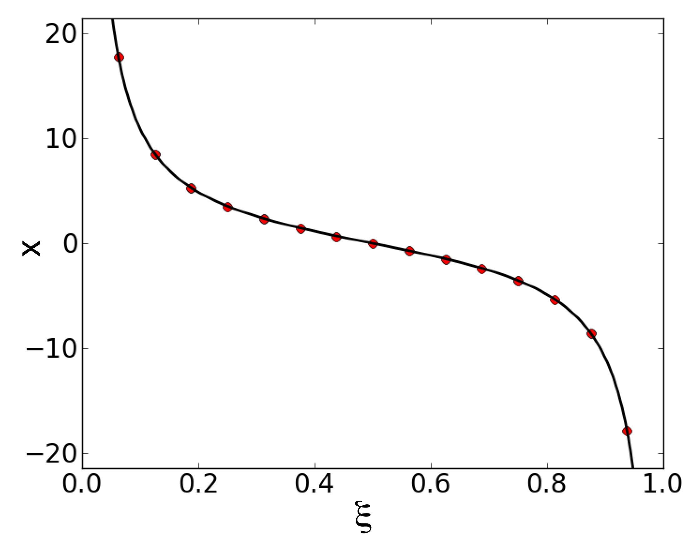
Fig. 10: Membrane potential values as a function of $\xi=i/N$ for a splay state. The symbols refer to $N=16$, while the solid line to the continuous limit approximation. The data have been obtained for $J=15$, $T_{s}=1$ ms and $\tau=20$ ms.

Appendix C Marginally stable directions of the splay states

In this appendix, we will analyze the stability of a splay state in the case of non-overlapping step pulses. To perform this analysis, let us rewrite the QIF model (1) as follows

$$\tau\frac{d\theta_{i}}{dt}=I(t)+(I(t)-2)\cos\theta_{i}\qquad i=1,\dots,N\qquad;$$ (77)

where we have performed the transformation of variable $\theta_{i}=2\tan^{-1}(v_{i})$. Therefore, the membrane potential is now represented by a a phase variable $\theta_{i}\in[-\pi;\pi]$, the spike is emitted (and transmitted instantaneously to all the neurons in the network) whenever $\theta_{i}$ reaches the threshold $\pi$ and then $\pi$ it is reset to $-\pi$. The model in the formulation (77) is termed $\theta$-neuron, we will apply the Watanabe and Strogatz [29] approach to this model to derive the Floquet spectrum for the splay state solution.

In order, to stress the peculiar PSPs we are considering, we rewrite (77) as follows

$$\frac{d\theta_{j}}{dt}=(J\phi(\mathbf{\theta})-2)\cos(\theta_{j})+J\phi(\mathbf{\theta})\qquad\qquad j=1,\ldots N$$ (78)

with $\phi(\theta)$ being the characteristic function of the interval $[-\pi,\theta_{OFF}]$. The emission of a spikes occurs whenever the neuron $\min\{\theta_{i}\}=-\pi$ this amounts to an increase by one in the value of the function $\phi(\theta)$. Furthermore, when the pulse expires after a time $T_{s}$ the value of $\phi(\mathbf{\theta})$ will be decreased by one. By assuming that no neuron will fire while the synapse is on (no overlapping PSPs), the PT will occur for a specific value of the phase variable namely $\min\{\theta_{i}\}=\theta_{OFF}$, for a value $\theta_{OFF}$, which can be determined as outlined in §3A.

Let us now recall the approach devised by Watanabe and Strogatz [29] to show that each trajectory representing the dynamics of a system of $N$ identical phase oscillators, whose evolution is ruled by ODEs of the form

$$\frac{d\theta_{j}}{dt}=f(\mathbf{\theta})+g(\mathbf{\theta})\cos(\theta_{j})+h(\mathbf{\theta})\sin(\theta_{j})\qquad\qquad j=1,\ldots N\quad,$$ (79)

is confined to a three dimensional subspace. The only requirement is that the functions $f$, $g$ and $h$ do not depend on the index $j$ of the considered oscillator. In other words $f$, $g$ and $h$ are collective variables determined by the network state. Clearly our equation (78) satisfies this condition.

Watanabe and Strogatz introduce a transformation $Q_{x}:R^{N}\rightarrow R^{N+3}$ from variables $\{\theta_{j}\}$ to variables $X\equiv(\Gamma,\Theta,\Psi,\{\psi_{j}\})$ defined implicitly by the set of equations

$$F(\theta_{j},\Gamma,\Theta,\Psi,\psi_{j})=0,\quad j=1,\ldots N\quad;$$ (80)

where

$$F=\tan\left(\frac{1}{2}(\theta_{j}-\Theta)\right)-\sqrt{\frac{1+\Gamma}{1-\Gamma}}\tan\left(\frac{1}{2}(\psi_{j}-\Psi)\right).$$ (81)

Furthermore, they prove that an arbitrary solution of (79) can be generated by the transformation $Q_{x}$ from a set of parameters $\{\psi_{j}\}$, which remain constant in time, whenever the three collective variables $\Gamma,\Theta,\Psi$ satisfy the following equations

$$\begin{split}&\dot{\Gamma}=-(1-\Gamma^{2})(g\sin\Theta-h\cos\Theta)\\ &\Gamma\dot{\Theta}=\Gamma f-g\cos\Theta-h\sin\Theta\\ &\Gamma\dot{\Psi}=\sqrt{1-\Gamma^{2}}(g\cos\Theta+h\sin\Theta)\qquad,\end{split}$$ (82)

and obviously the other variables satisfy

$$\dot{\psi}_{j}=0\qquad\forall j=1,\dots,N\qquad.$$ (83)

We prove the following proposition:

Proposition 1.

Let us assume that (78) admits a splay state solution and that this solution is Lyapunov stable. Then at least $N-2$ Floquet multipliers will lie on the unit circle.

Let us now recall the definition of the Floquet multipliers [7] for a generic ODE of the form

$$\dot{\mathbf{\theta}}=F_{x}(\mathbf{\theta}),\qquad\mathbf{\theta}\in R^{N}\quad,$$ (84)

admitting a periodic solution $\mathbf{\theta}^{s}(t)$ with period $T_{p}$.

The associated variational linear equation in the tangent space has the form:

$$\delta\dot{\mathbf{\theta}}=DF_{x}(\mathbf{\theta}^{s}(t))\delta\mathbf{\theta},\qquad\delta\mathbf{\theta}\in{\cal R}^{N}.$$ (85)

Equation (85) has (possibly complex) eigensolutions $\Phi(t)=e^{(\lambda+i\omega)t}\eta(t)$, with $\eta(t)$ periodic of period $T_{p}$, termed Floquet vectors. The complex numbers $\mu(T_{p})=e^{(\lambda+i\omega)T_{p}}$ are the Floquet multipliers. They determine the stability of the periodic solution.

Proof of 1. We will prove that there exists an $N-2$ dimensional subspace of solutions of the variational equation associated to (78) consisting of solutions that do not converge to the ${\bf 0}$ vector as $t\to\infty$ (except for the ${\bf 0}$ solution itself). This, combined with Lyapunov stability, implies that there must be $N-2$ Floquet multipliers on the unit circle.

Let $\mathbf{\theta}^{s}_{0}=\{\theta_{0,1}^{s},\ldots,\theta_{0,N}^{s}\}$ be a choice of initial conditions corresponding to a splay state of period $T_{p}$. For simplicity and without any loss of generality, we can assume that the phases are ordered, i.e. $\theta_{0,1}^{s}>\theta_{0,2}^{s}>\ldots,\theta_{0,N}^{s}$, and that $\theta_{0,1}^{s}$ is close to $\pi$, i.e. the first neuron is just about to fire.

Let us consider a solution $\mathbf{X}^{s}(t)$ of (82) and (83) with initial condition

$$\mathbf{X}^{s}_{0}=\{0,\frac{\pi}{2},\frac{\pi}{2},\theta_{0,1}^{s},\ldots,\theta_{0,N}^{s}\}\quad;$$ (86)

where it is evident that $\theta^{s}(t)=T_{x}(\mathbf{X}^{s}(t))$ since $T_{x}(\mathbf{X}^{s}(0))=\theta^{s}(0)$. Furthermore, we perturb the initial condition with a perturbation of the form

$$\Delta\psi=(\Delta\mathbf{\psi}_{1},\ldots,\Delta\psi_{N-2},0,0)\qquad,$$ (87)

in the following way

$$\mathbf{X}^{s}_{\Delta\psi}(0)=\mathbf{X}^{s}_{0}+\Delta\psi=\{0,\frac{\pi}{2},\frac{\pi}{2},\theta_{0,1}^{s}+\Delta\psi_{1},\ldots,\theta^{s}_{0,N-2}+\Delta\psi_{N-2},\theta_{0,N-1}^{s},\theta_{0,N}^{s}\}\qquad.$$ (88)

and we obtain the perturbed solutions $\mathbf{X}^{s}_{\Delta\psi}(t)$ at time $t$ by integrating (82) and (83), while the the corresponding solution of (79) is given by $\theta^{s}_{\Delta\psi}(t)=T_{x}(\mathbf{X}^{s}_{\Delta\psi}(t))$.

Let us denote the value of the perturbed orbit at integer multiples $k$ of the period $T_{p}$ as follows

$$\mathbf{X}^{s}_{\Delta\psi,k}=(\Gamma(kT_{p}),\Theta(kT_{p}),\psi(kT_{p}),\theta_{1}^{s}+\Delta\psi_{1},\ldots,\theta_{N-2}^{s}+\Delta\psi_{N-2},\theta_{N-1}^{s},\theta_{N}^{s})\quad,$$ (89)

and $\theta^{s}_{\Delta\psi,k}=T_{x}(\mathbf{X}^{s}_{\Delta\psi,k})$.

We will show that there exists a real positive constant $L$ such that, for every value of $k$,

$$\|\theta^{s}_{\Delta\psi,k}-\theta_{0}^{s}\|\geq L\|\Delta\mathbf{\psi}\|.$$ (90)

By assuming that the perturbation is sufficiently small, i.e. $||\mathbf{X}^{s}_{\Delta\psi,k}-\mathbf{X}_{0}^{s}||\ll 1$, we can approximate the evolution of the perturbed orbit in proximity of the unperturbed one, with the corresponding linearized dynamics, namely

$$T_{x}(\mathbf{X}^{s}_{\Delta\psi,k})-T_{x}(\mathbf{X}^{s}_{0})\approx DT_{x}(\mathbf{X}_{0}^{s})(\mathbf{X}^{s}_{\Delta\psi,k}-\mathbf{X}_{0}^{s})\qquad.$$ (91)

In order to write the Jacobian $DT_{x}(\mathbf{X}_{0}^{s})$, we need to estimate the following derivatives, which can be obtained by implicit differentiation of (80)

$$\frac{\partial\theta_{j}}{\partial\Theta}=1,\;\frac{\partial\theta_{j}}{\partial\Psi}=-1,\;\frac{\partial\theta_{j}}{\partial\gamma}=-\cos\theta_{j}^{s},\;\frac{\partial\theta_{j}}{\partial\psi_{k}}=\delta_{jk}.$$ (92)

where $\delta_{jk}$ is the Kronecker delta.

Let ${\bf V}^{0}\in{\cal R}^{N}$ be a vector with an unitary norm spanning a $N-2$ dimensional subspace and let assume that $\Delta{\bf\psi}=\sigma\mathbf{V}^{0}$ with $0<\sigma\leq 1$. We will prove that

$$\|\frac{1}{\sigma}DT_{x}(\mathbf{X}_{0}^{s})(\mathbf{X}^{s}_{\Delta\psi,k}-\mathbf{X}_{0}^{s})\|\geq L>0\qquad,$$ (93)

for some real constant $L$ independent of $\sigma$ and $k$.

By employing (92) the following expression can be derived

$$\frac{1}{\sigma}DT_{x}(\mathbf{X}_{0}^{s})(\mathbf{X}^{s}_{\Delta\psi,k}-\mathbf{X}_{0}^{s})=\left(\begin{array}[]{l}Z_{1}(k)/\sigma+V^{0}_{1}\\ Z_{2}(k)/\sigma+V^{0}_{2}\\ \quad\cdot\\ \quad\cdot\\ \quad\cdot\\ Z_{N-2}(k)/\sigma+V^{0}_{N-2}\\ Z_{N-1}(k)/\sigma\\ Z_{N}(k)/\sigma\end{array}\right)$$ (94)

where for brevity and clarity we set $Z_{j}(k)=v_{k}-z_{k}-\cos\theta_{j}^{s}v_{k}$ once redefined $v_{k}=\Gamma(kT_{p})$, $w_{k}=\Theta(kT_{p})-\frac{\pi}{2}$, and $z_{k}=\Psi(kT_{p})-\frac{\pi}{2}$. It is clear, due to their definition, that the components of the vector ${\bf Z}(k)=\{Z_{j}(k)\}$ are not linearly independent and in particular that they span a 2-dimensional subspace.

As a first step, the validity of the following inequality, $\forall k$ and for any sufficiently small $\sigma$, is discussed

$$|Z_{j}(k)|/\sigma=|(w_{k}-z_{k}-\cos\theta_{j}^{s}v_{k})|/\sigma\geq L\quad\mbox{for $j=N$ or $j=N-1$ }\qquad.$$ (95)

We consider two possible cases. In the first case, the inequality (95) holds, therefore (93) is satisfied since the length of any vector is bigger than the absolute value of one of its components, thus implying that the modulus of the l.h.s. of (94) would be greater than $L$ for any $k$ value.

In the second case, we assume that (95) does not hold uniformly in $k$ for $j=N$, and $j=N-1$, in other words the components $|Z_{N-1}(k)|/\sigma$ and $|Z_{N}(k)|/\sigma$ should converge to $0$ for $k\to\infty$ and $\sigma\to\infty$. Furthermore, since for $N>3$ $\cos\theta_{N}^{s}\neq\cos\theta_{N-1}^{s}$, each component $Z_{j}$ with $j=1,\ldots,N-2$ can be written as a linear combination of $Z_{N-1}$ and $Z_{N}$. This implies that each element $|Z_{N-1}(k)|/\sigma$ remains arbitrarily small $\forall j$ even for arbitrarily large (resp. small) $k$ (resp. $\sigma$). Now each component in the r.h.s. of (94) will have the form $Z_{j}/\sigma+V^{0}_{j}$ for $j=1,\ldots,N-2$, where the first quantity is arbitrarily small, but by construction the vector ${\bf V}^{0}$ has an unitary modulus, thus also in this second case (93) is satisfied for any $k$.

From the previous results it follows that the vector function

$${\bf V}(t)=\frac{d}{d\sigma}\theta_{\Delta\Psi}(t)|_{\sigma=0}$$ (96)

is a solution of the variational equation (85) which does not converge to $0$ as $t\to\infty$. Since (85) is a system of linear equations, a vector space of initial conditions gives rise to a vector space of solutions. Since ${\bf V}^{0}$ spans a $N-2$ dimensional vector space, which we denote by $LV$, our construction give a $N-2$ dimensional vector space of solutions of (85), which we denote by ${\cal LV}$.

As mentioned above the Floquet vectors are solutions of (85) of the form $\mu(t)\eta(t)$, with $\eta(t)$ periodic of period $T_{p}$ and $\mu(T_{p})$ the corresponding Floquet multipliers. Since we assumed that the examined periodic orbit (i.e. the splay state) is Lyapunov stable, the multipliers $\mu(T_{p})$ must be either on the unit circle or inside the unit circle. Without loss of generality, let us assume that at least two multipliers are inside the unit circle, otherwise the theorem would be automatically true.

Let denote by $LW$ the vector space spanned by the initial conditions of the two Floquet eigenvectors associated to the two multipliers which lie inside the unit circle and let ${\cal LW}$ be the corresponding vector subspace of solutions (spanned by the two Floquet eigenvectors). Since all non-zero solutions in ${\cal LW}$ converge to $0$ as $t\to\infty$ it follows that the intersection of $LW$ and $LV$ consists of the zero vector. Therefore, we can formally decompose any of the remaining $N-2$ Floquet vectors at initial time $t=0$ in two vectors, namely $\eta(0)={\bf W}_{1}(0)+{\bf V}_{1}(0)$ where ${\bf W}_{1}(0)\in LW$ and ${\bf V}_{1}(0)\in LV$. By linearity, if ${\bf W}_{1}(t)$ and ${\bf V}_{1}(t)$ are the solutions of (85) with initial conditions ${\bf W}_{1}(0)$ and ${\bf V}_{1}(0)$, it follows that $\eta(t)={\bf W}_{1}(t)+{\bf V}_{1}(t)$. If ${\bf V}_{1}(0)\neq{\bf 0}$ then $\eta(t)\not\in{\cal LW}$, moreover $\eta(t)$ does not converge to $0$ as $t\to\infty$ since ${\bf W}_{1}(t)$ does, while $V_{1}(t)$ does not. Therefore the corresponding Floquet multiplier can be only on the unit circle, due to our previous assumptions. Finally we have demonstrated that $N-2$ Floquet multipliers are on the unit circle and 2 are inside the unit circle.

References

- [1] L. F. Abbott and C. Van Vreeswijk, Asynchronous states in networks of pulse-coupled oscillators, Phys. Rev. E, 48 (1993), pp. 1483–1490.
- [2] D. J. Amit, Modeling brain function: The world of attractor neural networks, Cambridge University Press, Cambridge, 1992.
- [3] D. G. Aronson, M. Golubitsky, and M. Krupa, Coupled arrays of Josephson junctions and bifurcation of maps with symmetry, Nonlinearity, 4 (1991), pp. 861–902.
- [4] P. Ashwin, G. P. KIing, and J. W. Swift, Three identical oscillators with symmetric coupling, Nonlinearity, 3 (1990), pp. 585–601.
- [5] N. Brunel, Dynamics of sparsely connected networks of excitatory and inhibitory spiking neurons, J. Comput. Neurosci., 8 (2000), pp. 183–203.
- [6] M. Calamai, A. Politi, and A. Torcini, Stability of splay states in globally coupled rotators, Phys. Rev. E, 80 (2009), pp. 036209–1–9.
- [7] E. A. Coddington and N. Levinson, Theory of ordinary differential equations, Tata McGraw-Hill, London, 1972.
- [8] A. Compte, N. Brunel, P. S. Goldman-Rakic, and X.-J. Wang, Synaptic mechanisms and network dynamics underlying visuospatial working memory in a cortical network model, Cerebral Cortex, 10 (2000), pp. 910–923.
- [9] G. B. Ermentrout and N. Kopell, Parabolic bursting in an excitable system coupled with a slow oscillation, SIAM J. Appl. Math., 46 (1986), pp. 233–253.
- [10] S. Funahashi, C. J. Bruce, and P. S. Goldman-Rakic, Mnemonic coding of visual Space in the monkey s dorsolateral prefrontal cortex, J. Neurophysiol., 61 (1989), pp. 331–349.
- [11] J. M. Fuster and J. P. Jervey, Inferotemporal neurons distinguish and retain behaviorally relevant features of visual stimuli, Science, 212 (1981), pp. 952–955.
- [12] W. Gerstner and W. K. Kistler, Spiking neuron models, Cambridge University Press, Cambridfge, 2002.
- [13] D. Golomb, D. Hansel, B. Shraiman, and H. Sompolinsky, Clustering in globally coupled phase oscillators, Phys. Rev. A, 45 (1992), pp. 3516–3530.
- [14] B. S. Gutkin, C. R. Laing, C. Colby, C. C. Chow, and G. B. Ermentrout, Turning on and off with excitation: The role of spike-timing asynchrony and synchrony in sustained neural activity, J. Comp. Neurosci., 11 (2001), pp. 121–134.
- [15] P. Hadley and M. R. Beasley, Dynamical states and stability of linear arrays of Josephson junctions, App. Phys. Lett., 50 (1987), pp. 621-623.
- [16] V. Hakim and W.-J. Rappel, Dynamics of the globally coupled complex Ginzburg-Landau equation, Phys. Rev. A, 46 (1992), pp. R7347–R7350.
- [17] D. Hansel and G. Mato, Asynchronous states and the emergence of synchrony in large networks of interacting excitatory and inhibitory neurons, Neural. Comput., 15 (2003), pp. 1–56.
- [18] D. Hansel and G. Mato, Existence and stability of persistent states in large neuronal networks, Phys. Rev. Lett., 86 (2001), pp. 4175–4178.
- [19] D. Z. Jin, Fast convergence of spike sequences to periodic patterns in recurrent networks, Phys. Rev. Lett, 89 (2002), pp. 208102–1–4.
- [20] C. R. Laing and C. C. Chow, Stationary bumps in networks of spiking neurons, Neural. Comp., 13 (2001), pp. 1473–1494.
- [21] J. S. W. Lamb and J. A. G. Roberts, Time-reversal symmetry in dynamical systems: A survey, Physica D, 112 (1998), pp. 1–39.
- [22] S. Nichols and K. Wiesenfield, Ubiquitous neutral stability of splay-phase states, Phys. Rev. A, 45 (1992), pp. 8430–8345.
- [23] W.-J. Rappel, Dynamics of a globally coupled laser model, Phys. Rev. E, 49 (1994), pp. 2750–2755.
- [24] T. Seidel and B. Werner, Breaking the symmetry in a car-following model, Proc. Appl. Math. Mech., 6 (2006), pp. 657–658.
- [25] N. Spruston, P. Jonas, and B. Sakmann, Dendritic glutamate receptor channel in rat hippocampal CA3 and CA1 pyramidal neurons, J. Physiol., 482 (1995), pp. 325–352.
- [26] S. H. Strogatz and R. E. Mirollo, Splay states in globally coupled Josephson arrays: Analytical prediction of Floquet multipliers, Phys. Rev. E., 47 (1993), pp. 220–227.
- [27] K. Y. Tsang and I. B. Schwartz, Interhyperhedral diffusion in Josephson-junction arrays, Phys. Rev. Lett., 68 (1992), pp. 2265–2268.
- [28] C. Van Vreeswijk, Partial synchronization in populations of pulse-coupled oscillators, Phys. Rev. E, 54 (1996), pp. 5522–5537.
- [29] S. Watanabe and S. H. Strogatz, Constants of motion for superconducting Josephson arrays, Physica D, 74 (1994), pp. 197–253.
- [30] K. Wiesenfield, C. Bracikowski, G. James, and R. Roy, Observation of antiphase states in a multimode laser, Phys. Rev. Lett., 65 (1990), pp. 1749–1752.
- [31] R. Zillmer, R. Livi, A. Politi, and A. Torcini, Desynchronization in diluted neural networks, Phys. Rev. E, 74 (2006), pp. 036203–1–10.
- [32] R. Zillmer, R. Livi, A. Politi, and A. Torcini, Stability of the splay state in pulse-coupled networks, Phys. Rev. E, 76 (2007), pp. 046102–1–10.