Abstract

In this paper we discuss several results about the structure of the configuration space of two-dimensional tensegrities with a small number of points. We briefly describe the technique of surgeries that is used to find geometric conditions for tensegrities. Further we introduce a new surgery for three-dimensional tensegrities. Within this paper we formulate additional open problems related to the stratification space of tensegrities.

On stratifications for planar tensegrities with a small number of vertices

Oleg Karpenkov TU Graz, Kopernikusgasse 24, A8010, Graz, Austria karpenkov@tugraz.at Partially supported by RFBR SS-709.2008.1 grant and by FWF grant No. M 1273-N18.

Jan Schepers Departement Wiskunde, Katholieke Universiteit Leuven, Celestijnenlaan 200B, 3001, Leuven, Belgium janschepers1@gmail.com Postdoctoral Fellow of the Research Foundation - Flanders (FWO).

Brigitte Servatius Mathematics Department, Worcester Polytechnic Institute, 100 Institute Road, Worcester, MA 01609-2280, USA bservat@math.wpi.edu

52C30, 05C10

1 Introduction

In this paper we study the stratification spaces of tensegrities with a small number of points. We work mostly with planar tensegrities. In the case of 4 and 5 point configurations we give an explicit description of all the strata and present a visualization of the entire stratification space. Further we give a geometric description of the strata for 6 and 7 points and use the technique of surgeries to find new geometric conditions adding to the list of already known ones. In particular, we introduce a new surgery for tensegrities in $\mathbb{R}^{3}$.

1.1 Configuration space of tensegrities

The first steps in the study of rigidity and flexibility of tensegrities were made by B. Roth and W. Whiteley in [9] and further developed by R. Connelly and W. Whiteley in [3], see also the survey about rigidity in [13]. N. L. White and W. Whiteley in [12] started the investigation of geometric conditions for a tensegrity with prescribed bars and cables. In the preprint [7] M. de Guzmán describes several other examples of geometric conditions for tensegrities.

Let us recall standard definitions of tensegrities (as in [2], [4], etc.). See also [10] for a collection of open problems and a good bibliography.

Definition 1.

Fix a positive integer $d$. Let $G=(V,E)$ be an arbitrary graph without loops and multiple edges. Let it have $n$ vertices $v_{1},\ldots,v_{n}$.

• A configuration is a finite collection $P$ of $n$ labeled points $(p_{1},p_{2},\ldots,p_{n})$, where each point $p_{i}$ (also called a vertex) is in a fixed Euclidean space $\mathbb{R}^{d}$.

• The embedding of $G$ with straight edges, induced by mapping $v_{j}$ to $p_{j}$ is called a tensegrity framework and it is denoted as $G(P)$.

• We say that a load or force $F$ acting on a framework $G(P)$ in $\mathbb{R}^{d}$ is an assignment of a vector $f_{i}$ in $\mathbb{R}^{d}$ to each vertex $i$ of $G$.

• We say that a stress $w$ for a framework $G(P)$ in $\mathbb{R}^{d}$ is an assignment of a real number $w_{i,j}=w_{j,i}$ (we call it an edge stress) to each edge $p_{i}p_{j}$ of $G$. An edge stress is regarded as a tension or a compression in the edge $p_{i}p_{j}$. For simplicity reasons we put $w_{i,j}=0$ if there is no edge between the corresponding vertices. We say that $w$ resolves a load $F$ if the following vector equation holds for each vertex $i$ of $G$:

  $$f_{i}+\sum\limits_{\{j|j\neq i\}}w_{i,j}(p_{j}-p_{i})=0.$$

  By $p_{j}{-}p_{i}$ we denote the vector from the point $p_{i}$ to the point $p_{j}$.

• A stress $w$ is called a self stress if, the following equilibrium condition is fulfilled at every vertex $p_{i}$:

  $$\sum\limits_{\{j|j\neq i\}}w_{i,j}(p_{j}-p_{i})=0.$$

• A couple $(G(P),w)$ is called a tensegrity if $w$ is a self stress for the framework $G(P)$.

• If $w_{i,j}<0$ then we call the edge $p_{i}p_{j}$ a cable, if $w_{i,j}>0$ we call it a strut.

Let $W(n)$ denote the linear space of dimension $n^{2}$ of all edge stresses $w_{i,j}$. Consider a framework $G(P)$ and denote by $W(G,P)$ the subset of $W(n)$ of all possible self stresses for $G(P)$. By definition the set $W(G,P)$ is a linear subspace of $W(n)$.

Definition 2.

The configuration space of tensegrities corresponding to the graph $G$ is the set

$$\Omega_{d}(G):=\big{\{}(G(P),w)\,|\,P\in(\mathbb{R}^{d})^{n},w\in W(G,P)\big{\}}.$$

The set $\{G(P)\,|\,P\in(\mathbb{R}^{d})^{n}\}$ is said to be the base of the configuration space, we denote it by $B_{d}(G)$.

1.2 Stratification of the base of a configuration space of tensegrities

Suppose we have some framework $G(P)$ and we want to find a cable-strut construction on it. Then which edges can be replaced by cables, and which by struts? What is the geometric position of points for which given edges may be replaced by cables and the others by struts? These questions lead to the following definition.

Definition 3.

A linear fiber $W(G,P_{1})$ is said to be equivalent to a linear fiber $W(G,P_{2})$ if there exists a homeomorphism $\xi$ between $W(G,P_{1})$ and $W(G,P_{2})$, such that for any self stress $w$ in $W(G,P_{1})$ the self stress $\xi(w)$ satisfies

$$\operatorname{sgn}\big{(}\xi(w)\big{)}=\operatorname{sgn}\big{(}w\big{)}.$$

The described equivalence relation gives us a stratification of the base $B_{d}(G)=(\mathbb{R}^{d})^{n}$. A stratum is by definition a maximal connected set of points with equivalent linear fibers. In the paper [4] we prove that all strata are semialgebraic sets (which implies for instance that they are path connected).

The idea of this paper is to make the first steps in the study of particular configuration spaces of tensegrities. We present the techniques to find geometric conditions and open problems for further study that already arise in very simple situations of 9 point configurations.

Let us, first, make the following three general remarks.

GR1. The majority of the strata of codimension $k$ can be defined by algebraic equations and inequalities that define the strata of codimension 1. The exceptions here are mostly in high codimension (the simplest one is as follows: for two points connected by an edge there is no codimension 1 stratum, but there is one codimension 2 stratum corresponding to coinciding points; actually it is interesting to find the complete list of such exceptions). So the most important case to study is the codimension 1 case.

GR2. A stratification of a subgraph is a substratification of the original graph (i.e., each stratum for a subgraph is the union of certain strata for the original graph), hence below we skip the description of $B_{2}(G)$ for graphs with 5 vertices other than $K_{5}$.

GR3. For any stratum there exists a certain subgraph that locally identifies the stratum (i.e., for any point $x$ of the stratum there exists a neighborhood $B(x)$ such that any configuration in $B(x)$ has a nonzero self stress for the subgraph if and only if this point is on the stratum).

According to general remarks GR1 and GR2 the most interesting case is to study the strata of codimension 1 for the complete graph on $n$ vertices (denoted further by $K_{n}$). It is possible to find some of the strata of $K_{n}$ directly. For the other strata one, first, should find an appropriate subgraph that locally identifies the stratum, and then find appropriate surgeries (explained in Section 3) to reduce the complexity of the subgraph to find geometric conditions.

This paper is organized as follows. In Section 2 we study the stratification of configuration spaces of tensegrities in the plane with a small number of vertices. In Subsections 2.1 and 2.2 we briefly describe the trivial cases of two and three point configurations. Further in Subsections 2.3 and 2.4 we study the four and the five point cases. In each of the cases we describe the geometry and the number of strata. In addition we introduce the adjacency diagram of full dimension and codimension 1 strata. In Subsections 2.5 and 2.6 we describe geometric conditions for the codimension 1 strata of 6, 7, and 8 point tensegrities. In Section 3 we present the technique of surgeries to find geometric descriptions for the strata. In Subsection 3.1 we describe surgeries that do not change graphs, and in Subsection 3.2 we show a couple of surgeries in the two-dimensional case. We introduce a new three-dimensional surgery in Subsection 3.3. In conclusion, we formulate several open questions in Subsection 3.4.

2 Stratification of the space $B_{2}(K_{n})$ for small $n$

In this section we study the geometry of tensegrity stratifications for graphs with a small number of vertices. The cases of $n=2,3,4,5$ are studied in full detail. Starting from $n=6$ there are some gaps in the understanding of tensegrities. Still for $n=6,7,8$ the complete description of the geometric conditions for the strata is known, we briefly describe several results on them here (see [4] for more information).

2.1 Case of two points

Consider, first, the case of two points ($n=2$). There are only two graphs on two points: a complete one $K_{2}$ and a graph without edges (denote it by $G_{0,2}$).

All the fibers of the base $B_{2}(G_{0,2})=\mathbb{R}^{4}$ are of dimension 0, and, therefore, they are equivalent. Hence the stratification is trivial.

The complete graph $K_{2}$ here has only one edge. If two points of the graph do not coincide then the stress at this edge should be zero. When two points coincide then the stress at the edge can be arbitrary, and we have a one-dimensional set of solutions (i.e., a fiber). So the base $B_{2}(K_{2})=\mathbb{R}^{4}$ has a codimension 2 stratum (a 2-dimensional plane). The complement to this stratum is a stratum of codimension 0.

2.2 Three point configurations

There are four different types of graphs here: let $G_{i,3}$ be the graph with $i$ edges for $i=0,1,2,3$.

In cases $G_{0,3}$ and $G_{1,3}$ the base stratifications are the following direct products:

$$B_{2}(G_{0,3})=B_{2}(G_{0,2})\times\mathbb{R}^{2}\quad\hbox{and}\quad B_{2}(G_{1,3})=B_{2}(K_{2})\times\mathbb{R}^{2}.$$

So $B_{2}(G_{0,3})$ is trivial and $B_{2}(G_{1,3})$ has a 4-dimensional subspace and its complement as strata.

The base $B_{2}(G_{2,3})$ contains five strata. One of them corresponds to the configuration where three points coincide: the fiber here is 2-dimensional, this stratum is isometric to $\mathbb{R}^{2}$. There are three strata where one of the edges of the graph vanishes: they are isometric to $\mathbb{R}^{4}\setminus\mathbb{R}^{2}$. Finally, the complement to the union of these strata is the only stratum of maximal dimension. There are no nonzero tensegrities for a configuration in this stratum.

For the complete graph on three vertices we have, for the first time, codimension 1 strata. There are three codimension 1 strata, all of them correspond to the following configuration: three points are in one line. Different strata correspond to having a different point between the two others.

Let us briefly describe one of such strata. Let $P_{i}=(x_{i},y_{i})$ be the points of the graph ($i=1,2,3$). Then the condition that the three points are in a line is defined by a quadratic equation:

$$(x_{2}-x_{1})(y_{3}-y_{1})-(x_{3}-x_{1})(y_{2}-y_{1})=0$$

This quadric divides the space into two connected components: corresponding to positively and negatively oriented triangles.

To sum up we present for $B_{2}(K_{3})$ the following table.

Dimension of a stratum	0	1	2	3	4	5	6
Number of such strata	0	0	1	0	3	3	2

2.3 Stratification of $B_{2}(K_{4})$

In this subsection we restrict ourselves to the complete graph $K_{4}$ (for its subgraphs we apply the reasoning of GR2 above). A plane configuration of four points in general position admits a unique tensegrity (up to a multiplicative constant), which is called an atom. In [8] it was proved that any self stress for $K_{n}$ is a sum of self-stressed atoms in $K_{n}$ (i.e., a sum of certain $K_{4}\subset K_{n}$ with scalars). For $K_{4}$ there are exactly 14 strata of general position.

The strata of codimension 1 correspond to three of four points of the graph lying in a line. Actually in this case there is no jump of dimension of the fiber: there is also a unique (up to scalar) solution corresponding to the three points in a line. But the stresses on the edges from the fourth point are all zero, and hence a fiber of this stratum is not equivalent to general fibers. The number of such strata is 24.

In codimension 2 we have two different types of strata corresponding to

• four points in a line: the dimension of a fiber is 2 (twelve strata);

• two points coincide: the dimension of a fiber is 1 (twelve strata).

In codimension 3 there is one type of strata with configurations of four points in a line, two of which coincide. Six of them with the double point in the middle and twelve of them with the double point not in the middle.

In codimension 4, there are two types of strata:

• three points coincide (4 strata);

• two pairs of points coincide (3 strata).

And, finally, there is a codimension 6 stratum when all four points coincide. We remark that for none of the strata the fiber is 3-dimensional.

The cardinalities of strata are shown in the following table.

Dimension of a stratum	0	1	2	3	4	5	6	7	8
Number of strata	0	0	1	0	7	18	24	24	14

2.3.1 The space of formal configurations

Let us draw schematically the adjacency of the strata of maximal dimension via strata of codimension 1. The dimension of the stratification space is 8, let us reduce it to two via factoring by proper affine transformations. We will use the following simple proposition.

Proposition 4.

Invertible affine transformations of the plane do not change the equivalence class of a fiber $W(G,P)$. In other words if $P$ is a configuration and $T$ an invertible affine transformation of the plane then

$$W(G,P)\simeq W(G,T(P)).$$

∎

So instead of studying the stratification itself we restrict to the set of formal configurations with respect to proper affine transformations of the plane.

Definition 5.

We say that a four point configuration $v_{1},v_{2},v_{3},v_{4}$ is formal in one of the following cases:

i$)$ nondegenerate case: a configuration $P_{x,y,+}$ with vertices $v_{1}=(0,0)$, $v_{2}=(1,0)$, $v_{3}=(x,y)$, $v_{4}=(x,y{+}1)$ for arbitrary $(x,y)$.

ii$)$ nondegenerate case: a configuration $P_{x,y,-}$ with $v_{1}=(0,0)$, $v_{2}=(1,0)$, $v_{3}=(x,y)$, $v_{4}=(x,y{-}1)$ for arbitrary $(x,y)$.

iii$)$ degenerate case: a configuration $P_{\Delta,+}$ with $v_{1}=(0,0)$, $v_{2}=(1,0)$, $v_{3}=(0,1)$, $v_{4}=(\Delta,1)$ for an arbitrary $\Delta$.

iv$)$ degenerate case: a configuration $P_{\Delta,-}$ with $v_{1}=(0,0)$, $v_{2}=(1,0)$, $v_{3}=(0,-1)$, $v_{4}=(\Delta,-1)$ for an arbitrary $\Delta$.

v$)$ closure: we add two formal configurations $P_{\pm\infty}$ with vertices $v_{1}=(0,0)$, $v_{2}=(1,0)$, $v_{3}=(1,0)$, $v_{4}=(1,\pm\infty)$.

We denote the set of all formal configurations by $\Lambda_{4}$.

In some sense the space $\Lambda_{4}$ is the space of all codimension 0 and codimension 1 configurations factored by the group of proper affine transformations.

Proposition 6.

For any codimension 0 and codimension 1 configuration there exists a unique formal configuration to which the first configuration can be affinely deformed. ∎

The space $\Lambda_{4}$ is endowed with a natural topology of a quotient space.

Proposition 7.

There is a natural topology of a unit sphere $S^{2}$ for the set $\Lambda_{4}$.

Proof 2.1.

Let us introduce a topology of a unit sphere $S^{2}$ for $\Lambda_{4}$. Consider the configurations of case i) on the plane $z=1$: we identify the point $P_{x,y,+}$ with the point $(x,y,1)$. Consider the projection of this plane to the upper unit hemisphere $S^{2}$ from the origin. So we have a one to one correspondence between the configurations of case i) and the upper hemisphere.

Similarly we take the plane $z=-1$ for the case ii) identifying the point $(-x,-y,-1)$ with the configuration $P_{x,y,-}$ and projecting it to the lower hemisphere.

For the equator of the unit sphere we use all the other cases as asymptotic directions. First, we associate the configuration $P_{\Delta,+}$ with the point

$$(\cos(\pi-\operatorname{arccotan}\Delta),\sin(\pi-\operatorname{arccotan}\Delta),0).$$

Let us explain the topology at one of such points of the equator. Suppose we start with $P_{x,y,+}$. The transformation sending the first three points to $(0,0)$, $(1,0)$, and $(0,1)$ is linear with matrix

$$\left(\begin{array}[]{cc}1&-x/y\\ 0&1/y\\ \end{array}\right).$$

Then the image of the fourth point of $P_{x,y,+}$ is $(-x/y,1{+}1/y)$. While $x$ tends to infinity and $x/y$ tends to $\Delta$ the last point tends to $(-\Delta,1)$, and hence the configuration $P_{x,y,+}$ tends to $P_{-\Delta,+}$, as in the above formula.

Secondly, we associate $P_{\Delta,-}$ with the point

$$(\cos(-\operatorname{arccotan}\Delta),\sin(-\operatorname{arccotan}\Delta),0)$$

in a similar way.

Finally, we glue $P_{+\infty}$ and $P_{-\infty}$ to the points $(1,0,0)$ and $(-1,0,0)$ respectively.

So, the codimension 0 and 1 stratification of $B_{2}(K_{4})$ can be derived from the stratification of the sphere. We show the stereographic projection of $\Lambda_{4}$ from the point $(0,0,-1)$ to the plane $z=1$ on Figure 1. There are four types of strata of codimension 1, they correspond to the fact that certain three points are in a line. They separate the plane into 14 connected components. In each of the connected components we draw a typical type of configuration: $(v_{1},v_{2},v_{3},v_{4})$. Here $v_{1}$ is blue, $v_{2}$ is purple, $v_{3}$ is red and $v_{4}$ is green.

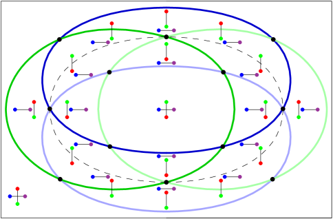
Figure 1: Stratification of $B_{2}(K_{4})$.

Remark 8.

Different geometric conditions are represented by different colors in the picture, the correspondence is as follows.

• Light blue strata (6 strata forming a circle) correspond to configurations with $v_{1}$, $v_{2}$, and $v_{3}$ in a line.

• Dark blue strata (6 strata) contain configurations with $v_{1}$, $v_{2}$, and $v_{4}$ in a line.

• Light green strata (6 strata) contain configurations with $v_{1}$, $v_{3}$, and $v_{4}$ in a line.

• Dark green strata (6 strata) correspond to configurations with $v_{2}$, $v_{3}$, and $v_{4}$ in a line. We have 24 strata of codimension 1 in total.

• The dashed black line is the projection of the equator. It corresponds to the degenerate case of parallel segments. The dashed line is not a stratum, it has the same fiber as all the points in its neighborhood. While one passes the dashed line the red-green segment ”rotates” around the blue-purple segment.

2.4 Stratification of $B_{2}(K_{5})$

2.4.1 General description of the strata

We have 264 strata of general position.

As in the two previous cases the strata of codimension 1 correspond to three points of the graph lying in a line. The number of such strata is 600.

The following strata are of codimension 2:

• twice three points in a line: 270 strata;

• four points in a line: 120 strata;

• two points coincide: 420 strata.

In codimension 3 we have the following cases:

• three points in a line and one double point: 60 strata;

• four points in a line two of which coincide: 180 strata;

• five points in a line: 60 strata.

For codimension 4 we have the following list:

• one triple point: 20 strata;

• five points in a line two of which coincide: 120 strata;

• two double points: 30 strata.

In codimension 5 we get:

• five points in a line three of which coincide: 30 strata;

• five points in a line with two pairs of points coinciding: 45 strata.

In codimension 6 there are the following strata:

• a triple point and a double point: 10 strata;

• one point and one point of multiplicity four: 5 strata.

And, finally, there is a codimension 8 stratum when all five points coincide.

The cardinalities of the strata are shown in the following table.

Dimension of a stratum	0	1	2	3	4	5	6	7	8	9	10
Number of strata	0	0	1	0	15	75	170	300	810	600	264

2.4.2 Visualization of $B_{2}(K_{5})$

Let us now describe the structure of the stratification $B_{2}(K_{5})$. Like in case of $B_{2}(K_{4})$ we introduce a set $\Lambda_{5}$ which represents the adjacency of strata of full dimension and of codimension 1. By definition we put

$$\Lambda_{5}=\Lambda_{4}\times\mathbb{R}^{2},$$

i.e., we consider all the four point configurations of $\Lambda_{4}$, and to each configuration we add the fifth point. We take the product topology for $\Lambda_{5}$.

So at each point of $\Lambda_{4}$ we attach an $\mathbb{R}^{2}$-fiber. It will soon become clear that for any full dimension stratum of $\Lambda_{4}$ the corresponding fibration is trivial, but the adjacency is not.

On Figures 2 and 3 we show $\Lambda_{5}$ in the following way. We draw the stratification of $\Lambda_{4}$ and inside each connected component we show the typical fiber of the component. The first four points are represented by purple, blue, green, and red points. The lines passing through any pair of them divide the fiber into 18 connected components, that correspond to strata of full dimension. At each such component we write a letter of the Latin alphabet (we consider capital and small letters as distinct).

• Two regions denoted by the same letter and lying in neighboring connected components of $\Lambda_{4}$ separated by light red, dark red, and black strata are in the same stratum.

• Two regions denoted by the same letter and lying in neighboring connected components of $\Lambda_{4}$ separated by light blue, dark blue, light green, and dark green strata are in distinct strata which are adjacent to the same codimension 1 stratum.

• Two regions denoted by a distinct letter and lying in neighboring connected components of $\Lambda_{4}$ are not in one stratum and are not adjacent to the same codimension 1 stratum.

The light blue, dark blue, light green, and dark green strata represent the same geometric conditions as in Remark 8 above. For the remaining strata we have:

• The dark red stratum symbolizes that the line through the red and blue points is parallel to the line through the green and purple points.

• The light red stratum symbolizes that the line through the red and purple points is parallel to the line through the green and blue points.

• The black stratum symbolizes that the line through the red and green points is parallel to the line through the purple and blue points.

Remark 9.

The configuration space $B_{2}(K_{5})$ has several obvious symmetries. First, there is the group of permutations $S_{5}$ that acts on the points of $B_{2}(K_{5})$; these symmetries are hardly seen from Figures 2 and 3 since the representation is not $S_{5}$-symmetric. Secondly, there is a symmetry about the origin that sends configurations from $B_{2}(K_{5})$ to themselves, on Figures 2 and 3 we used capital and small letters to indicate this symmetry (for instance, the strata of ”a” contain centrally symmetric configurations to the configurations of the strata ”A”).

Figure 2: Stratification of $B_{2}(K_{5})$ (Left part).

Figure 3: Stratification of $B_{2}(K_{5})$ (Right part).

As in the case of 4 point configurations we skip the subgraphs of $K_{5}$, see the second general remark above (GR2).

2.5 Essentially new strata in $B_{2}(K_{6})$

The stratification of $B_{2}(K_{6})$ is much more complicated, at this moment we do not even know how many strata of distinct dimension are present in the stratification.

According to GR1 the first step in studying the stratification of $B_{2}(K_{6})$ is to study all possible distinct types of strata of codimension 1. In the examples of $K_{n}$ for $n<6$ we only have strata corresponding to the following geometric condition: three points are in a line. For the case of 6 points we get two additional types of strata: six points on a conic, and three lines passing through three pairs of points have a unique point of intersection.

So the following are three codimension 1 strata (appeared in [12] by N. L. White and W. Whiteley):

• three points in a line;

• the lines $v_{1}v_{2}$, $v_{3}v_{4}$, and $v_{5}v_{6}$ meet in one point (or all parallel);

• all the six points are on a conic.

We conclude this subsection with the following problems.

Problem 10.

Find a description of $B_{2}(K_{6}),B_{3}(K_{4})$ and $B_{3}(K_{5})$ similar to the ones for $B_{2}(K_{4})$ and $B_{2}(K_{5})$ shown in the previous subsections.

2.6 A few words about the case $n>6$

In [4] we have studied strata of the 7 and 8 point configurations. There are 4 distinct types of codimension 1 strata for 7 points and 17 types for 8 points.

The 4 types of codimension 1 strata for 7 points are defined by the following geometric conditions:

• three points in a line;

• the lines $v_{1}v_{2}$, $v_{3}v_{4}$, and $v_{5}v_{6}$ meet in one point (or all parallel);

• the lines $v_{1}v_{2}$, $v_{3}v_{4}$, and $v_{5}p$ (where $p$ is the intersection of the lines $v_{2}v_{6}$ and $v_{3}v_{7}$) have a common nonempty intersection;

• the six points $v_{1}$, $v_{2}$, $v_{3}$, $v_{4}$, $v_{5}$, and $p$ (where $p$ is the intersection of the lines $v_{1}v_{6}$ and $v_{3}v_{7}$) are on a conic.

For the list of strata of 8 point configurations we refer to [4].

It turns out that the geometric conditions of any codimension 1 stratum can be obtained by the following procedure. Consider the points of configuration $P$; for each two pairs of points $(v_{i},v_{j})$ and $(v_{k},v_{l})$ of this configuration consider the point of intersection of the lines $v_{i}v_{j}$ and $v_{k}v_{l}$. This leads to a bigger configuration of points including $P$ and the above intersections, we denote it by $U(P)$. This operation can be iteratively applied infinitely many times, which results in a universal set

$$U^{\infty}(P)=\bigcup\limits_{m=0}^{\infty}U^{m}(P).$$

Any condition for a codimension 1 stratum is always as follows: three certain points of $U^{\infty}(P)$ are in a line (for the details, see for instance [9] and [4]).

Example 11.

The condition the lines $v_{1}v_{2}$, $v_{3}v_{4}$, and $v_{5}v_{6}$ meet in one point in terms of points of $U^{1}(P)=U(P)$ is as follows. The points $v_{1}$, $v_{2}$, and $p=v_{3}v_{4}\cap v_{5}v_{6}$ are in a line.

Remark 12.

For simplicity reasons we omit discussions of cases where certain lines $v_{i}v_{j}$ and $v_{k}v_{l}$ are parallel, due to the fact that this situation is never generic for codimension 1 strata. In general one may think that if the lines $v_{i}v_{j}$ and $v_{k}v_{l}$ are parallel, then their intersection point is in the line at infinity in the projectivization of $\mathbb{R}^{2}$.

Remark 13.

At first glance, the condition six points are on a conic is of different nature. Nevertheless, it is a relation on the points of the configuration in $U^{1}(P)$ described by Pascal’s theorem: The intersections of the extended opposite sides of a hexagon inscribed in a conic lie on the Pascal line. See also Example 17 below.

Problem 14.

Describe all the possible different types of strata for 9 points.

Problem 15.

How to calculate the number of different types of strata for $n$ points with arbitrary $n$?

It is also interesting to have an answer for the following question: how many iterations $($i.e., find the minimal $m$ for ${U^{m}(P)}$$)$ does one need to perform to describe all conditions for the codimension 1 strata of $n$-point configurations $P$?

Problem 16.

Which configurations of $U^{m}(P)$ define the same geometric condition?

This problem is a kind of question of finding generators and relations for the set of all conditions. Let us show one type of such ”relations” in the following example.

Example 17.

Consider the condition: six points $v_{1},v_{2},\ldots,v_{6}$ are on a conic. This condition is described by configurations contained in $U^{1}(P)$ via Pascal’s theorem:

The points $p,q,r$ are in a line for  $\left\{\begin{array}[]{l}p=v_{\sigma(1)}v_{\sigma(2)}\cap v_{\sigma(4)}v_{\sigma(5)}\\ q=v_{\sigma(2)}v_{\sigma(3)}\cap v_{\sigma(5)}v_{\sigma(6)}\\ r=v_{\sigma(3)}v_{\sigma(4)}\cap v_{\sigma(6)}v_{\sigma(1)}\\ \end{array}\right.,$

where $\sigma$ is an arbitrary permutation of the set of six elements. So, there are 60 different configurations of $U^{1}(P)$ defining the same geometric condition.

3 Further study of strata: surgeries

We now look into subgraphs contained in a particular stratum and ask the basic question on the dimension of the fiber.

Even graphs of very low connectivity admit non-zero tensegrities, for disconnected or one-connected graphs we may simply examine the connected or 2-connected components. Also 2-connected graphs may be decomposed via the 2-sum, see [11]: Consider graphs $G_{1}$ and $G_{2}$, their configurations $P_{1}$ and $P_{2}$ admitting tensegrities with $p_{1}q_{1}$ a cable in $G_{1}(P_{1})$ and $p_{2}q_{2}$ a strut in $G_{2}(P_{2})$. We form the 2-sum $G_{1}\bigoplus G_{2}$ by identifying $p_{1}$ with $p_{2}$ and $q_{1}$ with $q_{2}$ and removing the identified edge. We can inherit a configuration $P$ from $P_{1}$ and $P_{2}$ by fixing $P_{1}$ and properly dilating, rotating and translating $P_{2}$. It is clear that

$$\dim W(G_{1}\bigoplus G_{2},P)=\dim W(G_{1},P_{1})+\dim W(G_{2},P_{2})-1.$$

Since 2-sum decomposition is canonical, we can describe geometric conditions for 2-connected graphs by geometric conditions on their 3-blocks. For example the geometric condition for $G$ in Figure 4 is that the lines $v_{1}v_{2}$, $v_{3}v_{4}$, and $v_{5}v_{6}$ meet in one point.

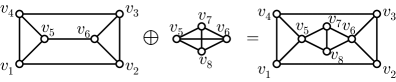
Figure 4: The 2-sum of a triangular prism with $K_{4}$

3.1 Subgraphs related to codimension 1 strata

As we have already mentioned in GR3, for any codimension 1 stratum there exists at least one subgraph of $K_{n}$ that generically does not admit tensegrities but at this stratum admits a one-dimensional family of tensegrities. Let us show such subgraphs for the codimension one strata of $B_{2}(K_{6})$ and $B_{2}(K_{7})$.

Example 18.

In the case of $K_{6}$ we have three strata of different geometrical nature. The first triangular subgraph (Figure 5, left) is related to the strata with three points in a line. The second (Figure 5, middle) corresponds to the strata whose three pairs of points generate lines passing through one point. The last one (Figure 5, right) corresponds to the configurations of six points on a conic.

            

Figure 5: Examples of subgraphs of $K_{6}$ admitting tensegrities at codimension 1 strata of $B_{2}(K_{6})$.

Example 19.

In the case of $K_{7}$ there are the following new examples of subgraphs, corresponding to the main 4 different types of strata.

From the left to the right we have the following geometric conditions

• $v_{1}$, $v_{2}$, and $v_{3}$ are in a line;

• the lines $v_{1}v_{2}$, $v_{3}v_{4}$, and $v_{5}v_{6}$ meet in one point;

• the lines $v_{1}v_{2}$, $v_{3}v_{4}$, and $v_{5}p$ (where $p=v_{2}v_{6}\cap v_{3}v_{7}$) have a common point;

• the six points $v_{1}$, $v_{2}$, $v_{3}$, $v_{4}$, $v_{5}$, and $p$ (where $p=v_{1}v_{6}\cap v_{3}v_{7}$) are on a conic.

         

Figure 6: Examples of subgraphs of $K_{7}$ admitting tensegrities at codimension 1 strata of $B_{2}(K_{7})$.

Note that the example for three points in a line is actually the 2-sum of a triangle with two atoms, so the only way for a non-zero self stress on the edges is to have $v_{1}$, $v_{2}$, and $v_{3}$, the vertices of the triangle, in a line.

Remark 20.

Geometric conditions for the graphs with 8 and fewer vertices are given in [4]. Several of those geometric conditions were described before in terms of bracket polynomials in [12] by N. L. White and W. Whiteley. We also refer to the paper [1] by E. D. Bolker and H. Crapo for the relation of bipartite graphs with rectangular bar constructions.

3.2 Surgeries on subgraphs that change geometric conditions in a predictable way

In this subsection we present several surgeries that allow to guess the geometric conditions for new strata (characterized by certain subgraphs) via other strata (characterized by these graphs modified in a certain way). We call such modifications of graphs surgeries.

3.2.1 Surgeries that do not change geometric conditions

Let $G$ be a graph, denote by $G_{e}$ the graph with an edge $e$ removed.

Proposition 21.

(Edge exchange) Consider a graph $G$ and a subgraph $H$, and let $e_{1}$ and $e_{2}$ be two edges of $H$. Let $P$ be a configuration for which $\dim W(H,P)=1$. Suppose also that the self stresses of $H$ do not vanish at the edges $e_{1}$ and $e_{2}$. Then we have

$$\dim W(G_{e_{1}},P)=\dim W(G_{e_{2}},P).$$

∎

In the situation of Proposition 21 the strata of $G_{e_{1}}(P)$ and $G_{e_{2}}(P)$ are defined by the same geometrical conditions.

3.2.2 Two two-dimensional surgeries that change geometric conditions

The first surgery is described in the following proposition.

Proposition 22.

Consider the frameworks $G(P)$, $G_{1}^{I}(P_{1}^{I})$, and $G_{2}^{I}(P_{2}^{I})$ as on the figure:

If none of the triples of points $(p,v_{2},v_{3})$, $(q,v_{2},v_{3})$, $(p,v_{2},v_{4})$, $(q,v_{3},v_{4})$ and $(v_{2},v_{3},v_{4})$ are on a line then we have

$$\dim W(G_{1}^{I},P_{1}^{I})=\dim W(G_{2}^{I},P_{2}^{I}).$$

Example 23.

Let us consider a simple example of how to get a geometric condition for the graph

to admit a tensegrity knowing all geometric conditions for 6-point graphs. Let us apply Surgery I to the points $v_{5}$, $v_{6}$, $v_{7}$. We have:

$$\epsfbox{table.5}\epsfbox{table.202}.$$

The geometric condition to admit a tensegrity for the graph on the right is:

the lines $v_{1}v_{2}$, $v_{3}v_{4}$ and $v_{5}p$ intersect in a point.
Hence the geometric condition for the original graph is:

the lines $v_{1}v_{2}$, $v_{3}v_{4}$ and $v_{5}p$ intersect in a point, where $p=v_{2}v_{6}\cap v_{3}v_{7}$.

Now let us show the second surgery.

Proposition 24.

Consider the frameworks $G(P)$, $G_{1}^{II}(P_{1}^{II})$, and $G_{2}^{II}(P_{2}^{II})$ as on the following figure:

If none of the triples of points $(p,q,v_{1})$, $(p,v_{1},v_{4})$, $(r,v_{1},v_{4})$, $(q,v_{1},v_{4})$, $(s,v_{1},v_{4})$, or $(r,s,v_{4})$ lie on a line then we have

$$\dim W(G_{1}^{II},P_{1}^{II})=\dim W(G_{2}^{II},P_{2}^{II}).$$

∎

Remark 25.

Both surgeries were shown in [4]. There is a certain analogy of the first surgery to $\Delta Y$ exchange in matroid theory (see for instance [13] and [5] for the connections between matroids and rigidity theory), but it is not exactly the same.

Remark 26.

Actually these surgeries are valid in the multidimensional case as well under the condition that certain points are in one plane.

3.3 A new tensegrity surgery in $\mathbb{R}^{3}$

We conclude this paper with a single surgery for tensegrities in $\mathbb{R}^{3}$.

Proposition 27.

Consider a graph $G$ and frameworks $G(P)$, $G_{1}(P_{1})$, and $G_{2}(P_{2})$ as follows:

Denote the plane $v_{2}v_{3}v_{4}$ by $\pi_{1}$. Suppose that the couples of edges $e_{1}$ and $e_{2}$, $e_{3}$ and $e_{4}$, $e_{5}$ and $e_{6}$ define planes $\pi_{2}$, $\pi_{3}$, and $\pi_{4}$, different from $\pi_{1}$. Assume that $\pi_{2}\cap\pi_{3}\cap\pi_{4}$ is a one point intersection.

If $G_{1}(P_{1})$ and $G_{2}(P_{2})$ have nonzero stress on the edges connecting $v_{1}$, $v_{2}$, $v_{3}$, and $v_{4}$ then

$$\pi_{1}\cap\pi_{2}\cap\pi_{3}\cap\pi_{4}=v_{1}.$$

In this case we additionally have

$$\dim W(G_{1},P_{1})=\dim W(G_{2},P_{2}).$$

Proof 3.1.

The first statement follows since $v_{1}$ only has valency 3 in $G_{2}(P_{2})$, so $v_{1}$, $v_{2}$, $v_{3}$, and $v_{4}$ need to be coplanar to have a nonzero edge stress. Now we explain how to map $W(G_{1},P_{1})$ to $W(G_{2},P_{2})$. The inverse map is simply given by the reverse construction. By the conditions $v_{1}$ is the intersection point of the planes $\pi_{1}$, $\pi_{2}$, and $\pi_{3}$. We add the uniquely defined plane atom on $v_{1},v_{2},v_{3},v_{4}$ to $G_{1}(P_{1})$ that cancels the edge stress on $v_{2}v_{3}$. Since the plane $\pi_{1}$ does not coincide with the plane $\pi_{2}$ spanned by the forces on $e_{1}$ and $e_{2}$, the edge stress on $v_{2}v_{4}$ is also canceled. By the same reasons the edge stress on $v_{3}v_{4}$ is canceled as well. This uniquely defines a self stress on $G_{2}(P_{2})$.

3.4 Some related open problems

The next goal in this approach is to continue to study the geometry of the strata. Ideally one would like to find techniques that will give geometric conditions for a graph via its combinatorics. This question seems to be a very hard open problem. The study of surgeries is the first step to solve it at least in codimension 1.

For a start we propose the following open question.

Problem 28.

Find all geometric conditions for the strata of 9 point tensegrities.

The surgeries introduced in this section were extremely useful for the study of 8 point configurations (see in [4]). We think that it is not enough to know only these surgeries to find all the geometric conditions. This gives rise to another question.

Problem 29.

Find other surgeries on graphs that predictably change the geometric conditions.

As far as we know there is no systematic study of strata for tensegrities in $\mathbb{R}^{3}$ or higher dimensions: these cases are much more complicated than the planar case. At least the stratification of $B_{3}(K_{5})$ should have a description similar to that of $B_{2}(K_{4})$, since 5 points in general position in $\mathbb{R}^{3}$ admit a unique non-zero self stress.

Additionally one should examine the rigidity properties of subgraphs in a stratum. For $K_{4}$ we have 14 strata of full dimension. For 8 of them the convex hull is a triangle, in 5 of the strata the points are in convex position. A tensegrity for the convex position has 4 struts (cables) and two cables (struts), while in the non-convex case there are three cables and three struts. All of these tensegrities are (infinitesimally) rigid and struts and cables may be exchanged without destroying rigidity. However, when viewed as graphs embedded in $\mathbb{R}^{3}$ only half of them are rigid. For the convex case, there must be cables on the convex hull and two struts. In the non-convex case there must be a triangle of struts on the convex hull and three cables in the interior, termed a spider web by R. Connelly. None of these are proper forms in the sense of B. Grünbaum. They are minimally rigid, but in the convex case they have members intersecting in a vertex other than a vertex of the graph, in the non-convex case there is a vertex without a strut. B. Grünbaum in his lectures on lost mathematics [6] asks about the number of proper forms given $n$ struts. On 3 struts, there is only one tensegrity which is minimally rigid with edges only intersecting at vertices and such that every vertex is endpoint of at least one strut. For 4 struts there are at least 20 forms, but it is not known how many there are. The number of forms on $n$ struts is bounded by the number of strata on $B_{3}(K_{n})$. For the hierarchies of the various kinds of rigidity see [3].

References

- [1] E. D. Bolker and H. Crapo, Bracing rectangular frameworks. I, SIAM J. Appl. Math. vol. 36, n. 3 (1979), pp. 473–490.
- [2] R. Connelly, Rigidity, Chapter 1.7 of Handbook of convex geometry, vol. A. Edited by P. M. Gruber and J. M. Wills, North-Holland Publishing Co., Amsterdam (1993), pp. 223–271.
- [3] R. Connelly and W. Whiteley, Second-order rigidity and prestress stability for tensegrity frameworks, SIAM Journal of Discrete Mathematics, vol. 9, n. 3 (1996), pp. 453–491.
- [4] F. Doray, O. Karpenkov, and J. Schepers, Geometry of configuration spaces of tensegrities, Discrete Comput. Geom., vol. 43, no. 2 (2010), pp. 436–466.
- [5] B. Jackson, T. Jordán, Connected rigidity matroids and unique realizations of graphs, J. Combin. Theory Ser. B, vol. 94, n. 1 (2005), pp. 1–29.
- [6] B. Grünbaum, Lectures on Lost Mathematics, lectures were given in 1975; the notes were digitized and reissued at the Structural Topology Revisited conference in 2006. http://hdl.handle.net/1773/15700 (2010)
- [7] M. de Guzmán, Finding Tensegrity Forms, preprint, 2004.
- [8] M. de Guzmán, D. Orden, From graphs to tensegrity structures: Geometric and symbolic approaches, Publ. Mat. 50 (2006), pp. 279–299.
- [9] B. Roth, W. Whiteley, Tensegrity frameworks, Trans. Amer. Math. Soc., vol. 265, n. 2 (1981), pp. 419–446.
- [10] B. Servatius, Tensegrities, PAMM, vol. 7, n. 1 (2007), pp. 1070101–1070102.
- [11] B. Servatius, H. Servatius, On the 2-sum in rigidity matroids, European J. Combin, vol. 32, n. 6 (2011), pp. 931–936.
- [12] N. L. White, W. Whiteley, The algebraic geometry of stresses in frameworks, SIAM J. Alg. Disc. Meth., vol. 4, n. 4 (1983), pp. 481–511.
- [13] W. Whiteley, Rigidity and scene analysis, in J. E. Goodman and J. O’Rourke, editors, Handbook of Discrete and Computational Geometry, chapt. 49, pp. 893–916, CRC Press, New York, 1997.