Modulus and Poincaré inequalities on non-self-similar Sierpiński carpets

Abstract.

A carpet is a metric space homeomorphic to the Sierpiński carpet. We characterize, within a certain class of examples, non-self-similar carpets supporting curve families of nontrivial modulus and supporting Poincaré inequalities. Our results yield new examples of compact doubling metric measure spaces supporting Poincaré inequalities: these examples have no manifold points, yet embed isometrically as subsets of Euclidean space.

1. Introduction

Metric spaces equipped with doubling measures that support Poincaré inequalities (also known as PI spaces) are ideal environments for first-order analysis and differential geometry [19], [10], [20], [23], [25]. Extending the scope of this theory by verifying Poincaré inequalities on new classes of spaces is a problem of high interest and relevance. Previously, several classes of spaces have been shown to support Poincaré inequalities:

• compact Riemannian manifolds or noncompact Riemannian manifolds satisfying suitable curvature bounds [9],

• Carnot groups and more general sub-Riemannian manifolds equipped with Carnot-Carathéodory (CC) metric [19], [18], [21],

• boundaries of certain hyperbolic Fuchsian buildings, see Bourdon and Pajot [6],

• Laakso’s spaces [28],

• linearly locally contractible manifolds with good volume growth [32].

These examples fall into two (overlapping) classes: examples for which the underlying topological space is a manifold, and abstract metric examples which admit no bi-Lipschitz embedding into any finite-dimensional Euclidean space. Such bi-Lipschitz nonembeddability follows from Cheeger’s celebrated Rademacher-style differentiation theorem in PI spaces, as explained in [10, §14]. Euclidean bi-Lipschitz nonembeddability is known, for instance, for all nonabelian Carnot groups and other regular sub-Riemannian manifolds, as well as for the examples of Bourdon and Pajot [6] and Laakso [28].

The preceding dichotomy should not be taken too seriously. Nonabelian Carnot groups equipped with the CC metric, for instance, have underlying space which is a topological manifold, yet do not admit any Euclidean bi-Lipschitz embedding. On the other hand, it is certainly possible to construct Euclidean subsets with some nonmanifold points which are PI spaces. This can be done, for instance, by appealing to various gluing theorems for PI spaces, see [19, Theorem 6.15] (reproduced as Theorem 2.2 in this paper) for a general result along these lines. However, the following question appears to have been unaddressed in the literature until now.

Question 1.1.

Do there exist sets $X\subset\mathbb{R}^{N}$ (for some $N$) with no manifold points which are PI spaces when equipped with the Euclidean metric and some suitable measure?

In connection with Question 1.1 we recall the examples constructed by Heinonen and Hanson [16]. For each $n\geq 2$, these authors construct a compact, geodesic, Ahlfors $n$-regular PI space of topological dimension $n$ with no manifold points. They suggest [16, p. 3380], but do not check, that their nonmanifold example admits a bi-Lipschitz embedding into some Euclidean space. Note that the question about embeddability of the Heinonen–Hansen example is not resolved by Cheeger’s work, since this example admits almost everywhere unique tangent cones coinciding with $\mathbb{R}^{n}$.

The examples of PI spaces due to Bourdon and Pajot [6] comprise a class of compact metric spaces arising as the Gromov boundaries of certain hyperbolic groups acting geometrically on Fuchsian buildings. Topologically, all of the Bourdon–Pajot examples are homeomorphic to the Menger sponge. It is well-known that ‘typical’ Gromov hyperbolic groups have Menger sponge boundaries. While examples of Gromov hyperbolic groups with Sierpiński carpet boundary do exist, it is not presently known whether any such boundary can verify a Poincaré inequality in the sense of Heinonen and Koskela.

Question 1.2.

Do there exist PI spaces that are homeomorphic to the Sierpiński carpet?

In this paper we answer Questions 1.1 and 1.2 affirmatively. We identify a new class of doubling metric measure spaces supporting Poincaré inequalities. Our main results are Theorem 1.5 and 1.6. Our spaces have no manifold points, indeed, they are all homeomorphic to the Sierpiński carpet. On the other hand, all of our examples arise as explicit subsets of the plane equipped with the Euclidean metric and the Lebesgue measure. These are the first examples of compact subsets of Euclidean space without interior that support Poincaré inequalities for the usual Lebesgue measure.

To fix notation and terminology we recall the notion of Poincaré inequality on a metric measure space as introduced by Heinonen and Koskela [19]. Let $(X,d,\mu)$ be a metric measure space, i.e., $(X,d)$ is a metric space and $\mu$ is a Borel measure which assigns positive and finite measure to all open balls in $X$. A Borel function $\rho:X\rightarrow[0,\infty]$ is an upper gradient of a function $u:X\rightarrow\mathbb{R}$ if $|u(x)-u(y)|\leq\int_{\gamma}\rho\,ds$ whenever $\gamma$ is a rectifiable curve joining $x$ to $y$.

Definition 1.3 (Heinonen–Koskela).

Fix $p\geq 1$. The space $(X,d,\mu)$ is said to support a $p$-Poincaré inequality if there exist constants $C,\lambda\geq 1$ so that for any continuous function $u:X\rightarrow\mathbb{R}$ with upper gradient $\rho:X\rightarrow[0,\infty]$, the inequality

(1.1) $$\mathchoice{{\vbox{\hbox{$\textstyle-$}}\kern-4.86108pt}}{{\vbox{\hbox{$\scriptstyle-$}}\kern-3.25pt}}{{\vbox{\hbox{$\scriptscriptstyle-$}}\kern-2.29166pt}}{{\vbox{\hbox{$\scriptscriptstyle-$}}\kern-1.875pt}}\!\int_{B}\left|u-\mathchoice{{\vbox{\hbox{$\textstyle-$}}\kern-4.86108pt}}{{\vbox{\hbox{$\scriptstyle-$}}\kern-3.25pt}}{{\vbox{\hbox{$\scriptscriptstyle-$}}\kern-2.29166pt}}{{\vbox{\hbox{$\scriptscriptstyle-$}}\kern-1.875pt}}\!\int_{B}u\,d\mu\right|\,d\mu\leq C\operatorname{diam}(B)\left(\mathchoice{{\vbox{\hbox{$\textstyle-$}}\kern-4.86108pt}}{{\vbox{\hbox{$\scriptstyle-$}}\kern-3.25pt}}{{\vbox{\hbox{$\scriptscriptstyle-$}}\kern-2.29166pt}}{{\vbox{\hbox{$\scriptscriptstyle-$}}\kern-1.875pt}}\!\int_{\lambda B}\rho^{p}\,d\mu\right)^{1/p}$$

holds for every ball $B=B(x,r)\subset X$. Here we denote, for a subset $E\subset X$ of positive measure, the mean value of a function $u:E\to\mathbb{R}$ by $\mathchoice{{\vbox{\hbox{$\textstyle-$}}\kern-4.86108pt}}{{\vbox{\hbox{$\scriptstyle-$}}\kern-3.25pt}}{{\vbox{\hbox{$\scriptscriptstyle-$}}\kern-2.29166pt}}{{\vbox{\hbox{$\scriptscriptstyle-$}}\kern-1.875pt}}\!\int_{E}u\,d\mu=\frac{1}{\mu(E)}\int_{E}u\,d\mu$.

The validity of a Poincaré inequality in the sense of Definition 1.3 reflects strong connectivity properties of the underlying space. Roughly speaking, metric measure spaces $(X,d,\mu)$ supporting a Poincaré inequality have the property that any two regions are connected by a rich family of relatively short curves which are evenly distributed with respect to the background measure $\mu$. (For a more precise version of this statement, see Theorem 2.1.) The main results of this paper are a reflection and substantiation of this general principle in the setting of a highly concrete collection of planar examples.

We now turn to a description of those examples. To each sequence $\mathbf{a}=(a_{1},a_{2},\ldots)$ consisting of reciprocals of odd integers strictly greater than one we associate a modified Sierpiński carpet $S_{\mathbf{a}}$ by the following procedure. Let $T_{0}=[0,1]^{2}$ be the unit square and let $S_{\mathbf{a},0}=T_{0}$. Consider the standard tiling of $T_{0}$ by essentially disjoint closed congruent subsquares of side length $a_{1}$. Let $\mathcal{T}_{1}$ denote the family of such subsquares obtained by deleting the central (concentric) subsquare, and let $S_{\mathbf{a},1}=\cup\{T:T\in\mathcal{T}_{1}\}$. Again, let $\mathcal{T}_{2}$ denote the family of essentially disjoint closed congruent subsquares of each of the elements of $\mathcal{T}_{1}$ with side length $a_{1}a_{2}$ obtained by deleting the central (concentric) subsquare from each square in $\mathcal{T}_{1}$, and let $S_{\mathbf{a},2}=\cup\{T:T\in\mathcal{T}_{2}\}$. Continuing this process, we construct a decreasing sequence of compact sets $\{S_{\mathbf{a},m}\}_{m\geq 0}$ and an associated carpet

$$S_{\mathbf{a}}:=\bigcap_{m\geq 0}S_{\mathbf{a},m}.$$

For example, when $\mathbf{a}=(\tfrac{1}{3},\tfrac{1}{3},\tfrac{1}{3},\ldots)$, the set $S_{\mathbf{a}}$ is the classical Sierpiński carpet $S_{1/3}$ (Figure 2). For any $\mathbf{a}$, $S_{\mathbf{a}}$ is a compact, connected, locally connected subset of the plane without interior and with no local cut points. By a standard fact from topology, $S_{\mathbf{a}}$ is homeomorphic to the Sierpiński carpet $S_{1/3}$.

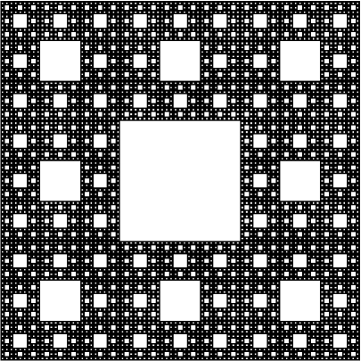
Figure 1. $S_{1/3}$

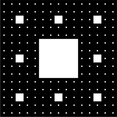
Figure 2. $S_{(1/3,1/5,1/7,\ldots)}$

For each $k\in\mathbb{N}$, we will denote by $S_{1/(2k+1)}$ the self-similar carpet $S_{\mathbf{a}}$ associated to the constant sequence $\mathbf{a}=(\tfrac{1}{2k+1},\tfrac{1}{2k+1},\tfrac{1}{2k+1},\ldots)$. For each $k$, the carpet $S_{1/(2k+1)}$ has Hausdorff dimension equal to

(1.2) $$Q_{k}=\frac{\log((2k+1)^{2}-1)}{\log(2k+1)}=\frac{\log(4k^{2}+4k)}{\log(2k+1)}<2$$

and is Ahlfors regular in that dimension.

The starting point for our investigations was the following well-known fact.

Proposition 1.4.

For each $k$, the carpet $S_{1/(2k+1)}$, equipped with Euclidean metric and Hausdorff measure in its dimension $Q_{k}$, does not support any Poincaré inequality.

Several proofs for Proposition 1.4 can be found in the literature. Bourdon and Pajot [7] provide an elegant argument involving the mutual singularity of one-dimensional Lebesgue measure and the push forward of the $Q_{k}$-dimensional Hausdorff measure on $S_{1/(2k+1)}$ under projection to a coordinate axis. A different argument involving modulus computations can be found in the monograph by the first two authors [29].

In this paper, we study non-self-similar carpets $S_{\mathbf{a}}$ for which $\mathbf{a}$ is not a constant sequence. We are primarily interested in the case when $S_{\mathbf{a}}$ has Hausdorff dimension two. It is easy to see that this holds, for instance, if the sequence $(a_{m})$ of scaling ratios tends to zero, i.e., $\mathbf{a}\in c_{0}$. Figure 2 illustrates the set $S_{(1/3,1/5,1/7,\ldots)}$.

Note that the left and right hand edges of $S_{\mathbf{a}}$ are separated by the generalized Cantor set

$$C_{\mathbf{a}}:=S_{\mathbf{a}}\cap\left(\big{\{}\tfrac{1}{2}\big{\}}\times[0,1]\right).$$

This Cantor set will have positive length if and only if the length at each stage, $\prod_{j=1}^{m}(1-a_{j})$, remains bounded away from zero. After taking logarithms, this is seen to be equivalent to $\mathbf{a}\in\ell^{1}$.

In a similar fashion, we see that $\operatorname{Area}(S_{\mathbf{a}})=\mathcal{H}^{2}(S_{\mathbf{a}})$ is positive if and only if $\operatorname{Area}(S_{\mathbf{a},m})=\prod_{j=1}^{m}(1-a_{j}^{2})$ is bounded away from zero, i.e., $\mathbf{a}\in\ell^{2}$.

We equip $S_{\mathbf{a}}$ with the Euclidean metric $d$ and the canonically defined measure $\mu$ arising as the weak limit of normalized Lebesgue measures on the precarpets $S_{\mathbf{a},m}$. For all $\mathbf{a}$, the measure $\mu$ is doubling. Under the assumption $\mathbf{a}\in\ell^{2}$, $\mu$ is Ahlfors $2$-regular and is comparable (with constant depending only on $||\mathbf{a}||_{2}$) to the restriction of Lebesgue measure to $S_{\mathbf{a}}$. For these and other facts, see Proposition 3.1.

We now state our main theorems.

Theorem 1.5.

The carpet $(S_{\mathbf{a}},d,\mu)$ supports a $1$-Poincaré inequality if and only if $\mathbf{a}\in\ell^{1}$.

Under the assumption of Theorem 1.5, the $1$-modulus of all horizontal paths in $S_{\mathbf{a}}$ is easily seen to be positive. This fact follows from the usual Fubini argument, since the cut set $C_{\mathbf{a}}$ has positive length. The difficult part of the proof of Theorem 1.5 is the verification of the $1$-Poincaré inequality. This is done using a theorem of Keith (Theorem 2.1) and a combinatorial procedure involving concatenation of curve families of positive $1$-modulus.

Theorem 1.6.

The following are equivalent:

1. $(S_{\mathbf{a}},d,\mu)$ supports a $p$-Poincaré inequality for each $p>1$,

2. $(S_{\mathbf{a}},d,\mu)$ supports a $p$-Poincaré inequality for some $p>1$,

3. $\mathbf{a}\in\ell^{2}$.

For $\mathbf{a}\in\ell^{2}\setminus\ell^{1}$, the $p$-modulus of all horizontal paths in $S_{\mathbf{a}}$ is equal to zero for any $p$. However, the $p$-modulus ($p>1$) of all rectifiable paths is positive. In section 6 we exhibit explicit path families with positive modulus. This provides a first step towards our eventual verification of the Poincaré inequality. Such verification in this context relies on the same theorem of Keith and a similar concatenation argument, starting from curve families of positive $p$-modulus as constructed above.

It is not unexpected, and seems to have been informally recognized, that a generalized Sierpiński carpet $S_{\mathbf{a}}$ admits some Poincaré inequalities, provided the sequence $\mathbf{a}$ tends to zero sufficiently rapidly. Indeed, if $\mathbf{a}$ tends rapidly to zero then the omitted squares at each stage of the construction occupy a vanishingly small proportion of their parent square; this leaves plenty of room in the complementary region to construct well distributed curve families. The essential novelty of Theorems 1.5 and 1.6 lies in their sharp character; we identify the precise summability conditions necessary and sufficient for the validity of the $p$-Poincaré inequality for each choice of $p\in[1,\infty)$. Note that, by Theorems 1.5 and 1.6, if $\mathbf{a}\in\ell^{2}\setminus\ell^{1}$, then $(S_{\mathbf{a}},d,\mu)$ supports a $p$-Poincaré inequality for each $p>1$, but does not support a $1$-Poincaré inequality. A significant recent result of Keith and Zhong [25] asserts that the set of values of $p$ for which a given complete PI space supports a $p$-Poincaré inequality, is necessarily a relatively open subset of $[1,+\infty)$.

Remarkably, the $\ell^{2}$ summability condition on the defining sequence $\mathbf{a}$ has recently arisen in a rather different (although related) context. To wit, Doré and Maleva [11] show that when $\mathbf{a}\in c_{0}\setminus\ell^{2}$, the compact set $S_{\mathbf{a}}$ is a universal differentiability set, i.e., it contains a differentiability point for every real-valued Lipschitz function on $\mathbb{R}^{2}$.

Theorems 1.5 and 1.6 have a number of interesting consequences which we now enunciate.

Corollary 1.7.

There exist compact planar sets of topological dimension one that are Ahlfors $2$-regular and $2$-Loewner when equipped with the Euclidean metric and the Lebesgue measure.

For each $\mathbf{a}\in\ell^{2}$, the carpet $S_{\mathbf{a}}$ verifies the conditions in Corollary 1.7. This follows from Theorem 1.6 and the equivalence of the $Q$-Loewner condition with the $Q$-Poincaré inequality in quasiconvex Ahlfors $Q$-regular spaces [19]. We remark that the examples of Bourdon–Pajot [6] and Laakso [28] are $Q$-regular $Q$-Loewner metric spaces of topological dimension one, however, these examples admit no bi-Lipschitz embedding into any finite-dimensional Euclidean space.

Corollary 1.8.

There exists a compact set $S\subset\mathbb{R}^{2}$, equipped with the Euclidean metric and a doubling measure, with the following properties: $S$ supports no $p$-Poincaré inequality for any finite $p$, yet every strict weak tangent of $S$ supports a $1$-Poincaré inequality with universal constants. Moreover, $S$ can be chosen to be quasiconvex and uniformly locally Gromov–Hausdorff close to planar domains.

It is a general principle of analysis in metric spaces that quantitative geometric or analytic conditions often persist under Gromov–Hausdorff convergence. In particular, quantitative and scale-invariant conditions pass to weak tangent spaces. For instance, every weak tangent of a given doubling metric measure space satisfying a $p$-Poincaré inequality is again doubling and satisfies the same $p$-Poincaré inequality (see Theorem 2.5 for a version of this result used in this paper). Corollary 1.8 shows that weak tangent spaces can be significantly better behaved than the spaces from which they are derived, even in the presence of other good geometric properties.

The indicated example can be obtained by choosing $S=S_{\mathbf{a}}$ for any $\mathbf{a}\in c_{0}\setminus\ell^{2}$. This follows from Theorem 1.6 and Proposition 4.4 discussed in section 4.1, where further details of the proof of Corollary 1.8 can be found.

A carpet is a metric measure space homeomorphic to $S_{1/3}$. There has been considerable interest of late in the problem of quasisymmetric uniformization of carpets by either round carpets or slit carpets [3], [4], [5], [31], [30]. The following results are additional consequences of Theorem 1.6.

Corollary 1.9.

There exist round carpets in $\mathbb{R}^{2}$ which are Ahlfors $2$-regular and support a $p$-Poincaré inequality for some $p<2$.

Corollary 1.10.

There exist parallel slit carpets which are Ahlfors $2$-regular and support a $p$-Poincaré inequality for some $p<2$.

Recall that a planar carpet is said to be a round carpet if all of its peripheral circles are round geometric circles. A slit carpet is a carpet which is a Gromov–Hausdorff limit of a sequence of planar slit domains equipped with the internal metric. Recall that a domain $D\subset\mathbb{C}$ is a slit domain if $D=D^{\prime}\setminus\bigcup_{i\in I}\gamma_{i}$, where $D^{\prime}$ is a simply connected domain and $\{\gamma_{i}\}_{i\in I}$ is a collection (of arbitrary cardinality) of disjoint closed arcs contained in $D^{\prime}$. We admit the possibility that some of these arcs are degenerate, i.e., reduce to a point. A slit domain, resp. a slit carpet, is parallel if the nondegenerate arcs are parallel line segments, resp. if it is a limit of parallel slit domains.

Corollaries 1.9 and 1.10 are proved in section 7. Corollary 1.9 follows from Theorem 1.6 and results of Bonk and Koskela–MacManus on quasisymmetric uniformization of carpets and quasisymmetric invariance of Poincaré inequalities on Ahlfors regular spaces. Corollary 1.10 follows from Theorem 1.6, Koebe’s uniformization theorem and the same work of Koskela–MacManus. Indeed, every carpet $S_{\mathbf{a}}$ with $\mathbf{a}\in\ell^{2}$ is quasisymmetrically equivalent to both a round carpet and also to a slit carpet with the stated properties.

1.1. Outline of the paper

In section 2 we recall general facts about analysis in metric spaces, particularly, facts about Poincaré inequalities in the sense of Definition 1.3. In section 3 we prove basic metric and measure-theoretic properties of the carpets $S_{\mathbf{a}}$. In particular, we show that the canonical measure on $S_{\mathbf{a}}$ is always a doubling measure, and we indicate in which situations it verifies upper or lower mass bounds.

Section 4 is devoted to the necessity of the $\ell^{2}$ summability condition for the validity of Poincaré inequalities on the carpets $S_{\mathbf{a}}$. The main result of this section, Proposition 4.2, shows that $\ell^{2}$ summability of $\mathbf{a}$ is best possible for such conclusions. We also describe in more detail the weak tangents of the carpets $S_{\mathbf{a}}$ and substantiate Corollary 1.8.

Our proofs of the sufficiency of the summability criteria in Theorems 1.5 and 1.6 are contained in sections 5 and 6, respectively. In the setting of Theorem 1.5, where $\mathbf{a}\in\ell^{1}$, the Cantor set corresponding to the thinnest part of the carpet has positive length. This enables us to give a combinatorial construction of parameterized curve families that joins arbitrary pairs of points in $S_{\mathbf{a}}$ and verifies a modulus lower estimate due to Keith (Theorem 2.1) known to be equivalent to the Poincaré inequality in a wide setting.

In the setting of Theorem 1.6, where $\mathbf{a}$ is only assumed to be in $\ell^{2}$, a different technique is required. The key step is to perform, in the special case of the carpets $S_{\mathbf{a}}$, the following abstract procedure: in a metric space $(X,d)$ endowed with a wide supply of rectifiable curves (in our case, $\mathbb{R}^{2}$), deform a given curve family so as to avoid a prespecified obstacle, at a small quantitative multiplicative cost to the $p$-modulus. Iterating this procedure produces curve families of positive $p$-modulus that avoid a countable family of obstacles of prespecified geometric sizes. Our implementation, while not completely general, covers a wider class of residual sets than just carpets: see Theorem 6.7 for a precise statement.

In both cases, our proof of the suitable Poincaré inequalities makes substantial use of the precise rectilinear structure of carpets. Hence, the validity of a Poincaré inequality on the more general class of residual sets indicated in the preceding paragraph is less clear.

In the final section (Section 7) we discuss uniformization of the carpets $S_{\mathbf{a}}$ by either round carpets or slit carpets. In particular, we establish Corollaries 1.9 and 1.10.

1.2. Acknowledgements

We are grateful to Mario Bonk for numerous discussions and especially for suggestions concerning uniformization of metric carpets. We also thank Jasun Gong and Hrant Hakobyan for very helpful remarks. We wish to extend particular thanks to the referee for an extremely careful reading of the paper and for his or her detailed and constructive input.

Research for this paper was performed while the first and third authors were at the University of Illinois and during visits of all three authors to the Mathematics Institute at the University of Bern. The hospitality of both institutions is gratefully appreciated.

2. Preliminaries

2.1. Basic definitions and notation

If $B=B(x,r)$ denotes a ball in a metric space $X=(X,d)$, we write $\lambda B$ for the dilated ball $B(x,\lambda r)$.

A metric measure space is a metric space $(X,d)$ equipped with a Borel measure $\mu$ that is finite and positive on balls. The measure $\mu$ is doubling if there exists a constant $C>0$ so that $\mu(B(x,2r))\leq C\mu(B(x,r))$ for all metric balls $B(x,r)$ in $X$. It is Ahlfors $Q$-regular for some $Q>0$ if there exists a constant $C>0$ so that $r^{Q}/C\leq\mu(B(x,r))\leq Cr^{Q}$ for all metric balls $B(x,r)$ in $X$ with $0<r<\operatorname{diam}X$. We say that $\mu$ is Ahlfors regular if it is Ahlfors $Q$-regular for some $Q>0$. It is well known that any Ahlfors $Q$-regular measure on a metric space is comparable to the Hausdorff $Q$-measure $\mathcal{H}^{Q}$, and hence that $\mathcal{H}^{Q}$ is also Ahlfors $Q$-regular in that case. Ahlfors regular measures are always doubling. Let us remark that we always denote by $\mathcal{H}^{s}$ the $s$-dimensional Hausdorff measure in any metric space; we normalize these measures so that $\mathcal{H}^{n}$ coincides with Lebesgue measure in $\mathbb{R}^{n}$.

A metric space $(X,d)$ is said to be quasiconvex if there exists a constant $C$ so that any pair of points $x,y\in X$ can be joined by a rectifiable path $\gamma$ whose length is no more than $Cd(x,y)$. A metric space is quasiconvex if and only if it is bi-Lipschitz equivalent to a length metric space.

Every doubling metric measure space admitting a Poincaré inequality is quasiconvex, see for instance [15] or [10]. By making use of quasiconvexity, we may assume that $\lambda=1$ in (1.1), at the cost of increasing the value of $C$ [15, Corollary 9.8].

2.2. Poincaré inequalities and moduli of curve families

The following result of Keith [22, Theorem 2] will be of great importance in this paper.

Theorem 2.1 (Keith).

Fix $p\geq 1$. Let $(X,d,\mu)$ be a complete, doubling metric measure space. Then $X$ admits a $p$-Poincaré inequality if and only if there exist constants $C_{1}>0$ and $C_{2}\geq 1$ so that

(2.1) $$d(x,y)^{1-p}\leq C_{1}\operatorname{mod}_{p}(\Gamma_{xy};\mu_{xy}^{C_{2}})$$

for every pair of distinct points $x,y\in X$.

Here $\operatorname{mod}_{p}(\Gamma_{xy};\mu_{xy}^{C})$ denotes the $p$-modulus of the curve family $\Gamma_{xy}$ joining $x$ to $y$, where the measure $\mu_{xy}^{C}$ is the symmetric Riesz kernel

$$\mu_{xy}^{C}(A)=\int_{A\cap B_{xy}^{C}}\frac{d(x,z)}{\mu(B(x,d(x,z)))}+\frac{d(y,z)}{\mu(B(y,d(y,z)))}d\mu(z),$$

where $B_{xy}^{C}=B(x,Cd(x,y))\cup B(y,Cd(x,y))$. We recall that

$$\operatorname{mod}_{p}(\Gamma;\nu):=\inf\int\rho^{p}\,d\nu$$

for a Borel measure $\nu$ on $(X,d)$. Here the infimum is taken over all nonnegative Borel functions $\rho$ which are admissible for $\Gamma$, i.e., for which $\int_{\gamma}\rho\,ds\geq 1$ for all locally rectifiable curves $\gamma\in\Gamma$. When $(X,d)$ is endowed with a fixed ambient measure $\mu$, we abbreviate $\operatorname{mod}_{p}\Gamma=\operatorname{mod}_{p}(\Gamma;\mu)$.

2.3. Poincaré inequalities and metric gluings

The Poincaré inequality (1.1) is maintained under metric gluings. The following is a special case of a more general theorem of Heinonen and Koskela [19, Theorem 6.15], see also [16, Theorem 3.3].

Theorem 2.2 (Heinonen–Koskela).

Let $X$ and $Y$ be locally compact Ahlfors $Q$-regular metric measure spaces, $Q>1$, let $A\subset X$ be a closed subset, and let $\iota:A\to Y$ be an isometric embedding. Let $p>1$. Assume that both $X$ and $Y$ support a $p$-Poincaré inequality and that the inequality

$$\min\left\{\mathcal{H}^{Q-1}_{\infty}(A\cap B_{X}(x,r)),\mathcal{H}^{Q-1}_{\infty}(\iota(A)\cap B_{Y}(y,r))\right\}\geq cr^{Q-1}$$

holds for all $x\in A$, $y\in\iota(A)$ and $0<r<\min\{\operatorname{diam}X,\operatorname{diam}Y\}$, where the constant $c>0$ is independent of $x$, $y$ and $r$. Then $X\cup_{A}Y$ supports a $p$-Poincaré inequality. The data for the $p$-Poincaré inequality on $X\cup_{A}Y$ depends quantitatively on the Ahlfors regularity and Poincaré inequality data of $X$ and $Y$, on $p$, and on the above constant $c$.

We recall that the metric gluing $X\cup_{A}Y$ is the quotient space obtained by imposing on the disjoint union $X\coprod Y$ the equivalence relation which identifies each $a\in A$ with its image $\iota(a)$. We equip this space with a natural metric which extends the metrics on $X$ and $Y$ as follows: for points $x\in X$ and $y\in Y$, let $d(x,y)=\inf\{d(x,a)+d(\iota(a),y):a\in A\}$. Observe that the $Q$-regular measures on $X$ and $Y$, respectively, combine to give a measure on $X\cup_{A}Y$ which is also $Q$-regular.

2.4. Gromov–Hausdorff convergence and weak tangents

A metric space $(X,d)$ is proper if closed and bounded sets are compact.

Definition 2.3.

A sequence of pointed proper metric measure spaces

$$\{(X_{n},x_{n},d_{n},\mu_{n})\}$$

converges to a pointed metric measure space $(X,x,d,\mu)$ if there exists a pointed proper metric space $(Z,z,\rho)$ and isometric embeddings $f_{n}:X_{n}\rightarrow Z$, $f:X\rightarrow Z$ so that $f_{n}(x_{n})=f(x)=z$ for all $n$, $(f_{n})_{\#}\mu_{n}\rightarrow f_{\#}\mu$ weakly, and $f_{n}(X_{n})\rightarrow f(X)$ in the following sense: for all $R>0,\epsilon>0$ there exists $N$ so that for all $n\geq N$, $f_{n}(X_{n})\cap B(z,R)$ is contained in the $\epsilon$-neighborhood of $f(X)$, and $f(X)\cap B(z,R)$ is contained in the $\epsilon$-neighborhood of $f_{n}(X_{n})$.

We emphasize that the spaces $X_{n}$, $X$ are not assumed to be compact. For the notion of pointed Gromov–Hausdorff convergence, see [22, §2.2] or [8, Chapter 7].

Definition 2.4.

Let $(X,d,\mu)$ be a proper metric measure space. A pointed proper metric measure space $(Y,y,\rho,\nu)$ is called a weak tangent of $(X,d,\mu)$ if there exists a sequence of points $\{x_{n}\}\subset X$ and constants $\delta_{n}>0$, $\lambda_{n}>0$, so that the pointed proper metric measure spaces $\{(X,x_{n},\frac{1}{\delta_{n}}d,\frac{1}{\lambda_{n}}\mu_{n})\}$ converge to $(Y,y,\rho,\nu)$.

We do not require that $\delta_{n}\rightarrow 0$. In the event that this occurs, we call the limit space a strict weak tangent of $(X,d,\mu)$. If $x_{n}=x\in X$ for all $n$, we call $(Y,y,\rho,\nu)$ a tangent to $X$ at $x$. The notion of strict tangent is defined similarly.

Poincaré inequalities persist under Gromov–Hausdorff convergence; see Cheeger [10, §9]. We state here a version of this result due to Keith [22], in a form which is suitable for our setting. For another version, see Koskela [26].

Theorem 2.5 (Cheeger, Koskela, Keith).

Suppose $X_{1}\supset X_{2}\supset\cdots$ are subsets of $\mathbb{R}^{2}$, and for each $n\in\mathbb{N}$, $\mu_{n}$ is a doubling measure supported on $X_{n}$, with uniform doubling constant. Let $X=\bigcap_{n\in\mathbb{N}}X_{n}$, and suppose that the measures $\{\mu_{n}\}$ converge weakly to a measure $\mu$ supported on $X$. If each $(X_{n},d,\mu_{n})$ supports a $p$-Poincaré inequality with uniform constants, then $(X,d,\mu)$ also supports a $p$-Poincaré inequality.

3. Definition and basic properties of the carpets $S_{\mathbf{a}}$

We review the construction of the carpets $S_{\mathbf{a}}$. Fix a sequence

$$\mathbf{a}=(a_{1},a_{2},\ldots)$$

where each $a_{m}$ is an element of the set $\{\frac{1}{3},\frac{1}{5},\frac{1}{7},\ldots\}$. Starting from the unit square $T_{0}=[0,1]^{2}$ we set the level parameter $m=1$ and iteratively apply the following two steps:

• Divide each current square into $a_{m}^{-2}$ essentially disjoint closed congruent subsquares, where $m$ denotes the current level parameter, and remove the central (concentric) subsquare from each square,

• Increase the level parameter $m$ by $1$.

We let $\mathcal{T}_{m}$ denote the collection of all remaining level $m$ squares. For each $m$, $\mathcal{T}_{m}$ consists of

$$\prod_{j=1}^{m}\left(a_{j}^{-2}-1\right)$$

essentially disjoint closed squares, each of side length

$$s_{m}:=\prod_{j=1}^{m}a_{j}.$$

The union of all squares in $\mathcal{T}_{m}$ is the level $m$ precarpet, denoted $S_{\mathbf{a},m}$. A peripheral square is a connected component of the boundary of a precarpet. Finally,

$$S_{\mathbf{a}}:=\bigcap_{m\geq 0}S_{\mathbf{a},m}=\bigcap_{m\geq 0}\bigcup\mathcal{T}_{m}.$$

Each carpet $S_{\mathbf{a}}$ is quasiconvex; this can be demonstrated using curves built by countable concatenations of horizontal and vertical segments. It is well-known that the usual Sierpiński carpet $S_{1/3}$ contains other nontrivial line segments, neither horizontal or vertical. Indeed, $S_{1/3}$ contains nontrivial line segments of each of the following slopes: $0$, $1/2$, $1$, $2$ and $\infty$. For an explicit description of the set of slopes of nontrivial line segments in all carpets $S_{\mathbf{a}}$ in terms of Farey fractions, see [13].

3.1. The natural measure on $S_{\mathbf{a}}$

There is a natural probability measure on $S_{\mathbf{a}}$. Since each precarpet $S_{\mathbf{a},m}$ has positive area, we define a measure $\mu_{m}$ on $[0,1]^{2}$ which is the Lebesgue measure restricted to the set $S_{\mathbf{a},m}$, renormalized to have total measure one. The sequence of measures $(\mu_{m})$ converges weakly to a probability measure $\mu$ with support $S_{\mathbf{a}}$. To see this, note that on each (closed) square $T$ of scale $s_{m}$ that is not discarded, we have $\mu_{n}(T)=\mu_{m}(T)$ for all $n\geq m$, since later renormalizations merely redistribute mass within $T$. Therefore,

$$\mu(T)=\mu_{m}(T)=\prod_{j=1}^{m}(a_{j}^{-2}-1)^{-1}=:v_{m}.$$

Moreover, for fixed $Q>0$,

$$\frac{\mu(T)}{s_{m}^{Q}}=\prod_{j=1}^{m}a_{j}^{2-Q}(1-a_{j}^{2})^{-1}.$$

Note that if all $a_{m}=1/(2k+1)$, then $\mu(T)=s_{m}^{Q_{k}}$ for all $T\in\mathcal{T}_{m}$ and $\dim S_{1/(2k+1)}=Q_{k}$. Here $Q_{k}$ denotes the value in (1.2).

The following proposition describes the basic properties of $\mu$. We write $a\lesssim b$ to mean that there exists a constant $C>0$ so that $a\leq Cb$, where $C$ depends only on the relevant data. Also, the notation $a\asymp b$ signifies that $a\lesssim b$ and $b\lesssim a$.

Proposition 3.1.

The metric measure space $(S_{\mathbf{a}},d,\mu)$ has the following properties:

1. For any $\mathbf{a}$, $\mu$ is a doubling measure.

2. For any $\mathbf{a}$, we have the lower mass bound $\mu(B(x,r))\gtrsim r^{2}$ for all $x$ and $r\leq 1$.

3. If $\mathbf{a}\in c_{0}$, then for any $Q<2$ we have $\mu(B(x,r))\lesssim r^{Q}$ for all $x$ and $r>0$, hence $\dim S_{\mathbf{a}}=2$.

4. If $\mathbf{a}\in\ell^{2}$, then $\mu$ is comparable to Lebesgue measure with constant depending only on $||\mathbf{a}||_{2}$. Moreover, in this case, $\mu$ is an Ahlfors $2$-regular measure on $S_{\bf a}$.

5. If $\mathbf{a}=(a_{m})$ is eventually constant (and equal to $\frac{1}{2k+1}$), then $\mu$ is comparable to the Hausdorff measure $\mathcal{H}^{Q_{k}}$ and is an Ahlfors $Q_{k}$-regular measure on $S_{\mathbf{a}}$.

For $x\in S_{\mathbf{a}}$ and $r>0$ define two integers $m(x,r)$ and $m(r)$ as follows:

1. $m(x,r)$ is the smallest integer $m$ so that there exists $T\in\mathcal{T}_{m}$ with $x\in T\subset B(x,r)$,

2. $m(r)$ is the smallest integer $m$ so that $s_{m}\leq r$.

First, an easy lemma:

Lemma 3.2.

For any $x$ and $r$, $m(\sqrt{2}r)\leq m(x,r)\leq m(\frac{r}{\sqrt{2}})+1$.

Proof.

If $T\in\mathcal{T}_{m(x,r)}$ satisfies $x\in T\subset B(x,r)$, then $\sqrt{2}s_{m(x,r)}=\operatorname{diam}T\leq\operatorname{diam}B(x,r)\leq 2r$ which implies that $s_{m(x,r)}\leq\sqrt{2}r$ and $m(\sqrt{2}r)\leq m(x,r)$. Since $x\in T$ for some $T\in\mathcal{T}_{m(r/\sqrt{2})+1}$, and $\operatorname{diam}{T}\leq\frac{r}{3}$, we have $m(x,r)\leq m(\frac{r}{\sqrt{2}})+1$. ∎

We will derive the various parts of Proposition 3.1 from the following

Proposition 3.3.

For each $x\in S_{\mathbf{a}}$ and $0<r\leq 1$,

$$\mu(B(x,r))\asymp h(r):=r^{2}\prod_{j=1}^{m(r)}\left(\frac{1}{1-a_{j}^{2}}\right).$$

Proof of Proposition 3.1.

Note that $m(r)$ is a decreasing function of $r$. Part (i) follows easily:

$$\mu(B(x,2r))\lesssim(2r)^{2}\prod_{j=1}^{m(2r)}\left(\frac{1}{1-a_{j}^{2}}\right)\leq 4r^{2}\prod_{j=1}^{m(r)}\left(\frac{1}{1-a_{j}^{2}}\right)\lesssim\mu(B(x,r)).$$

Part (ii) is also clear, since the finite product term in the definition of $h(r)$ is always greater than or equal to one.

Next, we assert that $m(r)\leq m(2r)+1$ for all $r>0$. If not, we have $m(r)\geq m(2r)+2$, so $m(r)-1\geq m(2r)+1$, thus

$$r<s_{m(r)-1}\leq s_{m(2r)+1}\leq\frac{1}{3}s_{m(2r)}\leq\frac{1}{3}\cdot 2r,$$

a contradiction.

We now turn to part (iii). Assume that $\mathbf{a}\in c_{0}$, i.e., $a_{m}\to 0$. We will show that $\limsup_{r\to 0}\frac{\mu(B(x,r))}{r^{Q}}$ is finite for each $Q<2$, uniformly in $x$. It suffices to show that

$$\limsup_{r\to 0}\frac{h(r)}{r^{Q}}<\infty.$$

First we verify that $m(r)\leq-\log_{2}(r)+1$. Suppose that $n$ is the largest integer so that $2^{n}r\leq 1$. Since $m(1)=0$,

$$m(r)\leq m(2r)+1\leq\cdots\leq m(2^{n+1}r)+n+1\leq m(1)+n+1=n+1\leq-\log_{2}(r)+1.$$

Now, since $a_{j}\to 0$, for any $\epsilon>0$ there exists some $C=C(\epsilon)$ so that

$$\prod_{j=1}^{m(r)}\left(\frac{1}{1-a_{j}^{2}}\right)\leq C(1+\epsilon)^{m(r)}\leq C(1+\epsilon)^{-\log_{2}{r}+1}\lesssim r^{-\log_{2}(1+\epsilon)}.$$

If we choose $\epsilon$ so that $2-Q>\log_{2}(1+\epsilon)$, then we are done. From here part (iii) follows easily. Parts (iv) and (v) were discussed in the introduction. ∎

Proof of Proposition 3.3.

It is straightforward to bound $\mu(B(x,r))$ from above: cover $B(x,r)$ by squares from $\mathcal{T}_{m(r)}$. Then, as $s_{m(r)}\leq r$,

$$\mu(B(x,r))\leq\frac{(3r)^{2}}{s_{m(r)}^{2}}\cdot v_{m(r)}\leq\frac{9r^{2}}{s_{m(r)}^{2}}\cdot s_{m(r)}^{2}\prod_{j=1}^{m(r)}\left(\frac{1}{1-a_{j}^{2}}\right)\lesssim h(r).$$

To bound $\mu(B(x,r))$ from below, we split the proof into two cases.

Case 1.

$r\leq 100s_{m(x,r)}.$

Since $B(x,r)$ contains a square of side $s_{m(x,r)}$, we use the obvious bound $\mu(B(x,r))\geq v_{m(x,r)}$. Note that $m(r)-1\leq m(\frac{r}{\sqrt{2}})-1\leq m(\sqrt{2}r)\leq m(x,r)$. Now,

$$v_{m(x,r)}=s_{m(x,r)}^{2}\prod_{j=1}^{m(x,r)}\left(\frac{1}{1-a_{j}^{2}}\right)\geq\left(\frac{1}{100}\right)^{2}r^{2}\cdot(1-a_{m(r)}^{2})\prod_{j=1}^{m(r)}\left(\frac{1}{1-a_{j}^{2}}\right)\gtrsim h(r).$$

Case 2.

$r>100s_{m(x,r)}.$

Choose $T\in\mathcal{T}_{m(x,r)-1}$ so that $x\in T$. Since $T\nsubseteq B(x,r)$, the side length of $T$ is at least $\frac{r}{\sqrt{2}}$. Since $T$ is a square, $T\cap B(x,r)$ contains a (Euclidean) square $V^{\prime}$ of side $\frac{r}{4}$. Finally, since $s_{m(x,r)}\leq\frac{r}{100}$ and at most one square of generation $m(x,r)$ is deleted in $T$, $V^{\prime}$ contains a square $V$ of side $s_{v}\in[\frac{r}{32},\frac{r}{16}]$ consisting entirely of squares from $\mathcal{T}_{m(x,r)}$.

From the preceding facts we conclude that

$$\mu(B(x,r)) \geq\mu(V)=\left(\frac{s_{v}}{s_{m(x,r)}}\right)^{2}v_{m(x,r)}=s_{v}^{2}\cdot\prod_{j=1}^{m(x,r)}\left(\frac{1}{1-a_{j}^{2}}\right)$$

$$\geq\frac{r^{2}}{32^{2}}\cdot(1-a_{m(r)}^{2})\prod_{j=1}^{m(r)}\left(\frac{1}{1-a_{j}^{2}}\right)\gtrsim h(r).$$

The proof is finished. ∎

We make a final observation regarding the conformal dimension of $S_{\mathbf{a}}$. Recall that a metric space $(X,d)$ is minimal for conformal dimension if its Hausdorff dimension is less than or equal to the Hausdorff dimension of any quasisymmetrically equivalent metric space. The self-similar carpets $S_{1/(2k+1)}$ are not minimal for conformal dimension. This result is a consequence of a theorem of Keith and Laakso [24], see also [29] for a brief recapitulation of the proof.

Corollary 3.4.

If $\mathbf{a}\in c_{0}$, then $S_{\mathbf{a}}$ is minimal for conformal dimension.

Proof.

By Proposition 3.1(iii), $S_{\mathbf{a}}$ has Hausdorff dimension 2. In a similar way, one shows that the Cantor set $C_{\mathbf{a}}$ has Hausdorff dimension 1. Since $S_{\mathbf{a}}$ contains the product of $C_{\mathbf{a}}$ and an interval, which has Hausdorff dimension 2, by [2, Section 5, Remark 1] the space $S_{\mathbf{a}}$ is minimal for conformal dimension. ∎

The conformal dimensions of the carpets $S_{\mathbf{a}}$ when $\mathbf{a}\not\in c_{0}$ remain unknown. Determining the conformal dimension of $S_{1/3}$ is a longstanding open problem.

4. Failure of the Poincaré inequality

In this section we provide conditions under which the $p$-Poincaré inequality fails to be satisfied on $S_{\mathbf{a}}$ for various choices of $p$ and $\mathbf{a}$. In doing so we verify the necessity of the summability criteria in Theorems 1.5 and 1.6.

Proposition 4.1.

If $\mathbf{a}\notin\ell^{1}$, then $S_{\mathbf{a}}$ does not support a $1$-Poincaré inequality.

Proof.

For each $m\in\mathbb{N}$, let $T_{m}\subset S_{\mathbf{a}}$ be the vertical middle strip of width $s_{m}$. Define $f_{m}:S_{\mathbf{a}}\rightarrow[0,1]$ to be the function which is $0$ to the left of $T_{m}$, $1$ to the right of $T_{m}$ and extend it linearly across $T_{m}$. This function has upper gradient $\rho_{m}:S_{\mathbf{a}}\rightarrow[0,\infty]$ which is identically $1/{s_{m}}$ on $T_{m}$ and $\rho_{m}\equiv 0$ elsewhere. We compute

$$\int\rho_{m}\,d\mu=\prod_{i=1}^{m}\left(a_{i}^{-1}\cdot\frac{a_{i}-a_{i}^{2}}{1-a_{i}^{2}}\right)=\prod_{1}^{m}\frac{1}{1+a_{i}}.$$

Since $\mathbf{a}\notin\ell^{1}$, the right hand side goes to zero as $m\rightarrow\infty$. Observe that $\mathchoice{{\vbox{\hbox{$\textstyle-$}}\kern-4.86108pt}}{{\vbox{\hbox{$\scriptstyle-$}}\kern-3.25pt}}{{\vbox{\hbox{$\scriptscriptstyle-$}}\kern-2.29166pt}}{{\vbox{\hbox{$\scriptscriptstyle-$}}\kern-1.875pt}}\!\int_{S_{\mathbf{a}}}f_{m}d\mu=1/2$, and $f_{m}$ takes values of $0$ and $1$ on a set of measure bounded away from zero independently of $m$. Therefore, (1.1) cannot be satisfied for $p=1$ and fixed constant $C$. ∎

We now consider $p$-Poincaré inequalities with $p>1$. If $\mathbf{a}\not\in\ell^{3}$, a careful adaptation of the proof of the previous proposition shows that $S_{\mathbf{a}}$ does not support any Poincaré inequality. However, the carpets considered in this paper have a very specific geometry that leads to the following sharp result.

Proposition 4.2.

If $\mathbf{a}\notin\ell^{2}$, then $S_{\mathbf{a}}$ does not support a $p$-Poincaré inequality for any $p\geq 1$.

Proof.

Our goal is to build a set $X\subset S_{\mathbf{a}}$ with $\mu(X)=0$ so that for every rectifiable curve $\gamma$ joining the left and right hand edges of $S_{\mathbf{a}}$ we have $\int_{\gamma}\rho\,ds\geq 1$, where $\rho$ is the characteristic function of $X$.

This suffices to show the failure of the Poincaré inequality, for we can then define a function $f$ on $S_{\mathbf{a}}$ by letting $f(x)$ be the infimum of $\int_{\gamma}\rho\,ds$, where $\gamma$ ranges over all rectifiable curves joining the left edge of $S_{\mathbf{a}}$ to $x$. As $\rho\leq 1$ and $S_{\mathbf{a}}$ is quasi-convex, $f$ is a Lipschitz function which is zero on the left edge of $S_{\mathbf{a}}$. The property described above shows that $f\geq 1$ on the right edge of $S_{\mathbf{a}}$. Since $f$ has an upper gradient with essential supremum zero, we have a contradiction to (1.1).

In the remainder of the proof we build the set $X$ and show it has the desired properties for some fixed, arbitrary rectifiable curve $\gamma$ in $S_{\mathbf{a}}$ that joins the left and right hand edges of $S_{\mathbf{a}}$. By passing to a subcurve if necessary we may assume that $\gamma$ is an arc, i.e., that it is injective.

As part of our proof we shall build cut sets which disconnect $S_{\mathbf{a}}$. To simplify our discussion later, we define the set $H_{\mathbf{a}}$ to be the union of sets $[a,b]\times(c,d)$, for every deleted open square $(a,b)\times(c,d)$ in the construction of $S_{\mathbf{a}}$.

Initial step.

Let $A_{0}=S_{\mathbf{a}}$, and $\Gamma_{0}=\{\gamma\}$.

We divide $S_{\mathbf{a}}$ into $m_{1}=s_{1}^{-1}$ vertical strips of width $a_{1}$. These strips are bounded by vertical cut sets $V_{0},V_{1},\ldots,V_{m_{1}}$, where $V_{0}=(\{0\}\times[0,1])\setminus H_{\mathbf{a}},V_{1}=(\{a_{1}^{-1}\}\times[0,1])\setminus H_{\mathbf{a}}$, and so on. In other words, each $V_{j}$ is a vertical line, with the exception that the interiors of vertical sides of the deleted square of side $a_{1}$ are not contained in the appropriate $V_{j}$.

We now split $\Gamma_{0}=\{\gamma\}$ into a disjoint family of curves. We parametrize $\gamma$ by the interval $[0,1]$, with $\gamma(0)\in V_{0}$, and $\gamma(1)\in V_{m_{1}}$. Let $t_{0}^{+}\geq 0$ be the last time $\gamma$ meets $V_{0}$. Let $t_{1}^{-}>t_{0}^{+}$ be the next time after that $\gamma$ meets $V_{1}$. Let $\gamma_{1}$ be the subpath of $\gamma$ given by restricting to $[t_{0}^{+},t_{1}^{-}]$.

Continue inductively, letting $t_{j-1}^{+}\geq t_{j-1}^{-}$ be the last time $\gamma$ meets $V_{j-1}$, and $t_{j}^{-}>t_{j-1}^{+}$ be the next time $\gamma$ meets $V_{j}$. Let $\gamma_{j}$ be the subpath of $\gamma$ given by $[t_{j-1}^{+},t_{j}^{-}]$.

By construction, $\Gamma_{1}=\{\gamma_{1},\ldots,\gamma_{m_{1}}\}$ is a family of curves, where each $\gamma_{j}$ joins $V_{j-1}$ to $V_{j}$, and is contained between them. (See Figure 3, where the deleted subpaths are indicated by dotted lines.)

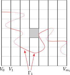
Figure 3. Curve splitting

Note that the length of $\Gamma_{1}$ (i.e., the sum of the lengths of $\gamma_{1},\ldots,\gamma_{m_{1}}$), is at least one and at most the length of $\Gamma_{0}$, that is $\operatorname{length}(\gamma)$.

Inductive step (fold in).

Fix $i\geq 1$. We are given as input a collection $\Gamma_{i}=\{\gamma_{j}\}$ of $m_{i}=s_{i}^{-1}$ curves and vertical slices $V_{0},\ldots,V_{m_{i}}$, where $\gamma_{j}$ joins $V_{j-1}$ to $V_{j}$ and is contained between them, for each $j=1,\ldots m_{i}$.

Choose the largest $l_{i}\in\mathbb{N}$ so that $l_{i}a_{i+1}\leq\frac{1}{3}$. Note that since $a_{i+1}\in\{\frac{1}{3},\frac{1}{5},\ldots\}$, we have $l_{i}a_{i+1}>\frac{1}{3}-\frac{1}{5}$.

Let $\mathcal{D}_{i}$ be the collection of open rectangles of width $l_{i}a_{i+1}s_{i}$ and height $(1-2l_{i}a_{i+1})s_{i}$ centered on and adjacent to either the left or right sides of the deleted squares of side length $s_{i}$. Consider the squares of side length $l_{i}a_{i+1}s_{i}$ above and below each of these rectangles. Each such square $S$ has a diagonal which meets the corner of a deleted square of side length $s_{i}$. This diagonal divides $S$ into two triangles; let $\mathcal{R}_{i}$ be the collection of closures of those triangles that share a side with a deleted square of side $s_{i}$. See Figure 4 for part of an example where these regions are labeled. We use the convention that the rectangles and triangles referred to are actually the intersection of the corresponding planar set and the carpet $S_{\mathbf{a}}$.

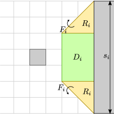
Figure 4. Unfolding

We now define a folding map $F_{i}:S_{\mathbf{a}}\rightarrow S_{\mathbf{a}}$ by declaring $F_{i}$ to be the identity except on $\cup\mathcal{R}_{i}$, where the map folds each triangle $R\in\mathcal{R}_{i}$ across the diagonal. Note that the horizontal edges of every rectangle in $\mathcal{D}_{i}$ are mapped to vertical edges, and that $F_{i}$ is discontinuous along such edges.

Notice that in Figure 4, if $a_{i+1}<\frac{1}{3}$ then the region $\cup\mathcal{D}_{i}$ will not overlap with $\cup\mathcal{D}_{i+1}$. However, when $a_{i+1}=\frac{1}{3}$, $\mathcal{D}_{i}$ may contain a square $Q$ of side length $s_{i+1}$ adjacent to the left or right of a particular deleted square of side length $s_{i+1}$, but it cannot contain both such squares. When this happens, we leave the square $Q$ untouched at step $i+1$, and do not include any part of it in $\mathcal{D}_{i+1}$.

We apply $F_{i}$ to the collection of curves $\Gamma_{i}$. Consider the resulting collection of curves. (Note that some curves have been broken into smaller pieces along the discontinuities of $F_{i}$.) We now build $\Gamma_{i+1}$ using the same inductive construction as we used in the initial step to build $\Gamma_{1}$ from $\Gamma_{0}$. As before, let $V_{j}=(\{js_{i+1}\}\times[0,1])\setminus H_{\mathbf{a}}$, for $j=0,\ldots,m_{i+1}$, separate the unit square into essentially disjoint vertical strips of width $s_{i+1}$. Here $m_{i+1}:=s_{i+1}^{-1}$. We define times

$$0\leq t_{0}^{+}<t_{1}^{-}\leq t_{1}^{+}<\cdots$$

as before, for the broken curve $F_{i}(\Gamma_{i})$.

Let $\gamma_{j}$ be the broken curve in $F_{i}(\Gamma_{i})$ given by the restriction to $[t_{j-1}^{+},t_{j}^{-}]$. In fact, $\gamma_{j}$ is connected.

By construction, $\Gamma_{i+1}=\{\gamma_{1},\ldots,\gamma_{m_{i+1}}\}$ is a family of curves, where each $\gamma_{j}$ joins $V_{j-1}$ to $V_{j}$, and is contained between them.

Moreover, $\Gamma_{i+1}$ will lie inside $A_{i}=\overline{A_{i-1}\setminus\cup(\mathcal{D}_{i}\cup\mathcal{R}_{i})}$. To see why this is so, consider (for example) $j$ so that $V_{j}$ lies on the left edge of a rectangle $D$ in $\mathcal{D}_{i}$, where $D$ lies on the left of an omitted square of side length $s_{i}$. By definition, $t_{j}^{+}$ is the last time the broken curve $F_{i}(\Gamma_{i})$ meets $V_{j}$. This corresponds to the last time that $\Gamma_{i}$ meets either $V_{j}$ or the horizontal edges of any element of $\mathcal{D}_{i}$ above or below $D$. Consequently, the family $\Gamma_{i+1}$ is disjoint from $\cup\mathcal{D}_{i}$ and (by the definition of $F_{i}$) it is also disjoint from the interior of $\cup\mathcal{R}_{i}$. As before, the length of $\Gamma_{i+1}$ is at least one and at most the length of $\Gamma_{i}$.

Conclusion.

We continue this construction until $i=n$, when we have a collection of curves $\Gamma_{n+1}$ that lies in $A_{n}$, and have deleted the rectangles in the collections $\mathcal{D}_{1},\ldots,\mathcal{D}_{n}$ from the sides of the deleted squares. We let $X_{n}^{(n)}=A_{n}$, and now proceed to unfold this set and the curves $\Gamma_{n+1}$ back out into the regions $\cup\mathcal{R}_{1},\ldots,\cup\mathcal{R}_{n}$.

Define inductively

$$X_{n}^{(i-1)}=F_{i}^{-1}(X_{n}^{(i)}),$$

for $i=n,n-1,\ldots,1$. Observe that $X_{n}^{(0)}$ is all of $S_{\mathbf{a}}$, but with certain rectangles removed that are adjacent to sides of removed squares of $S_{\mathbf{a},n}$.

It is clear that $S_{\mathbf{a}}=X_{0}^{(0)}\supset X_{1}^{(0)}\supset X_{2}^{(0)}\supset\cdots$. Let $X=\bigcap_{i=0}^{\infty}X_{i}^{(0)}$. For each $n$, and for any $\gamma$ in $\Gamma$, our construction implies that

$$\operatorname{length}(\gamma\cap X_{n}^{(0)}) =\operatorname{length}(\Gamma_{0}\cap X_{n}^{(0)})\geq\operatorname{length}(\Gamma_{1}\cap X_{n}^{(0)})$$

$$\geq\operatorname{length}(\Gamma_{2}\cap X_{n}^{(1)})\geq\cdots\geq\operatorname{length}(\Gamma_{n+1}\cap X_{n}^{(n)})$$

$$=\operatorname{length}(\Gamma_{n+1}\cap A_{n})\geq 1,$$

since $\Gamma_{n+1}$ is a chain of paths crossing each vertical strip of width $s_{n+1}$ from the left to the right, and $\Gamma_{n+1}$ lives in $A_{n}$.

Therefore, $\operatorname{length}(\gamma\cap X)\geq 1$, since $\operatorname{length}=\mathcal{H}^{1}$ is a measure on arcs.

Let $\rho$ be the characteristic function of $X$. Since $\gamma$ was an arbitrary rectifiable curve joining the left and right sides of $S_{\mathbf{a}}$, and $X$ was constructed independently of $\gamma$, we have shown that $\int_{\gamma}\rho\,ds\geq 1$ for every such curve $\gamma$.

It remains to prove that $\mu(X)=0$. Consider each deleted square of side $s_{i}$. Out of the neighboring $(a_{i}^{-2}-1)$ boxes of side $s_{i}$, from at least one (two if $a_{i}\neq\frac{1}{3}$) of these we will delete a rectangle in $\mathcal{D}_{i}$ whose $\mu$-measure, as a proportion of a square of side $s_{i}$, is at least $(1-2l_{i}a_{i+1})l_{i}a_{i+1}\geq\frac{2}{45}$. Since all the rectangles in $\mathcal{D}_{i}$ are pairwise disjoint, we have

$$\mu(X)\leq\prod_{i=1}^{\infty}\left(1-\frac{1}{a_{i}^{-2}-1}\cdot\frac{2}{45}\right)=\prod_{i=1}^{\infty}\left(1-\frac{2}{45}a_{i}^{2}+\cdots\right),$$

which converges to zero since $\mathbf{a}\notin\ell^{2}$. This completes the proof. ∎

Remark 4.3.

The argument also shows that $S_{\mathbf{a}}$ does not support an $\infty$-Poincaré inequality. See [12] for the definition, which is weaker than the $p$-Poincaré inequality for any finite $p$.

4.1. Weak tangents of Sierpiński carpets

Weak tangents of metric spaces describe infinitesimal behavior at a point or along a sequence of points. In this section we characterize the strict weak tangents of non-self-similar carpets. More precisely, we prove the following proposition.

Proposition 4.4.

Let $\mathbf{a}\in c_{0}$. Then every strict weak tangent of $S_{\mathbf{a}}$ is of the form $(\mathbb{R}^{2}\setminus T,d,\nu)$ where $T$ is a generalized square and $\nu$ is proportional to Lebesgue measure restricted to $\mathbb{R}^{2}\setminus T$.

By a generalized square we mean a set $T\subsetneq\mathbb{R}^{2}$ of the type

$$T=(a,b)\times(c,d)$$

where $-\infty\leq a\leq b\leq\infty$, $-\infty\leq c\leq d\leq\infty$, and $b-a=d-c$ if one (hence both) of these values is finite. (We interpret the degenerate interval $(a,b)$, $a=b$, as the empty set.) Thus $T$ is either the empty set, an open square, a quadrant or a half-space.

Suppose $W$ is a strict weak tangent arising as the limit of the sequence of metric spaces $\{X_{n}=(S_{\mathbf{a}},x_{n},\frac{1}{\delta_{n}}d)\}$, where $x_{n}\in S_{\mathbf{a}}$, $\delta_{n}\in(0,\infty)$, and $\delta_{n}\rightarrow 0$.

The following lemma indicates why $W$ can omit at most one large square.

Lemma 4.5.

There exist $R_{n}\rightarrow\infty$ and $r_{n}\rightarrow 0$ so that in the ball $B(x_{n},R_{n})\subset X_{n}$ there is at most one square of side greater than $1$ removed, and all other squares removed have size at most $r_{n}$.

Proof.

Fix $n$, and let $m=m(\delta_{n})$, i.e., $s_{m}\leq\delta_{n}<s_{m-1}$.

Either $\delta_{n}\in[s_{m},s_{m-1}\sqrt{a_{m}})$, or $\delta_{n}\in[s_{m-1}\sqrt{a_{m}},s_{m-1})$. In the first case, removed squares of size at least $\frac{s_{m}}{\delta_{n}}$ are $\frac{s_{m-1}}{2\delta_{n}}\geq\frac{1}{2\sqrt{a_{m}}}$ separated, while all others have size at most $\frac{s_{m+1}}{\delta_{n}}\leq a_{m+1}$. In the second case, removed squares of size at least $\frac{s_{m-1}}{\delta_{n}}\geq 1$ are $\frac{s_{m-2}}{2\delta_{n}}\geq\frac{1}{2a_{m-1}}$ separated, and all others have size at most $\frac{s_{m}}{\delta_{n}}\leq\sqrt{a_{m}}$.

Setting $R_{n}=\tfrac{1}{4}\min\{\frac{1}{a_{m-1}},\frac{1}{\sqrt{a_{m}}}\}$ and $r_{n}=\max\{\sqrt{a_{m}},a_{m+1}\}$, we have proved the lemma. ∎

Proof of Proposition 4.4.

Using the preceding lemma, we can reduce the proof of Proposition 4.4 to consideration of limits of $\mathbb{R}^{2}\setminus T_{n}$ where $T_{n}$ is either a square of side at least one, or the empty set. It is easy to see that any strict weak tangent $W$ as above will be isometric to $\mathbb{R}^{2}\setminus T$, where $T$ is either a square (of side at least one), a quarter-plane, half-plane or the empty set.

Since the measure $\mu$ on $S_{\mathbf{a}}$ agrees with the weak limit of renormalized Lebesgue measure on the domains $S_{\mathbf{a},m}$, by the lemma, if we look at measures of balls in $X_{n}$ of size much larger than $r_{n}$, they will agree with a constant multiple of Lebesgue measure up to small error. Consequently, the possible measures on $W$ will arise as limits of rescaled Lebesgue measure on $\mathbb{R}^{2}\setminus T_{n}$. The only possible non-trivial Radon measure of this type is a constant multiple of Lebesgue measure restricted to $\mathbb{R}^{2}\setminus T$. This finishes the proof of Proposition 4.4. ∎

Note that all of the weak tangent spaces identified in the conclusion of Proposition 4.4 support a $1$-Poincaré inequality, with uniform constants (i.e., independent of the choice of such a weak tangent space). This is because we have only a finite number of similarity types of spaces (full space, half space, quarter space, or the complement of a square), and the Poincaré inequality data is invariant under similarities. The quasiconvexity of the original carpets $S_{\mathbf{a}}$ is a standard fact. Indeed, arbitrary pairs of points can be joined by quasiconvex curves which are comprised of countable unions of horizontal and vertical line segments.

Definition 4.6.

A metric space $(X,d)$ is locally Gromov–Hausdorff close to planar domains if for each $x\in X$ and each $\epsilon>0$, there exists $r>0$ and a domain $\Omega\subset\mathbb{R}^{2}$ so that the Gromov–Hausdorff distance between the metric ball $B(x,r)\subset X$ and $\Omega$ is at most $\epsilon$. Furthermore, $(X,d)$ is uniformly locally Gromov–Hausdorff close to planar domains if $\epsilon$ can be chosen independently of $x$.

The fact that $S_{\mathbf{a}}$ is uniformly locally Gromov–Hausdorff close to planar domains follows easily from the construction and the condition $\mathbf{a}\in c_{0}$.

The preceding discussion and Theorem 1.6 understood, the proof of Corollary 1.8 is complete by the choice of $\mathbf{a}\in c_{0}\setminus\ell^{2}$.

5. Validity of the Poincaré inequality: the case $\mathbf{a}\in\ell^{1}$

In this section, we make the standing assumption that $\mathbf{a}\in\ell^{1}$, and show that $S_{\mathbf{a}}$, equipped with the Euclidean metric and the canonical measure described in subsection 3.1, admits a $1$-Poincaré inequality. Recall that whenever $\mathbf{a}$ is in $\ell^{2}\subset\ell^{1}$, Proposition 3.1(iv) states that $\mu$ is comparable to Hausdorff $2$-measure $\mathcal{H}^{2}$ restricted to $S_{\mathbf{a}}$. For simplicity we will work with $\mathcal{H}^{2}$ in this section and the next.

According to Theorem 2.1, the validity of a Poincaré inequality is equivalent to the existence of curve families of uniformly and quantitatively large weighted modulus joining arbitrary pairs of points. The desired curve family must spread out as it escapes from the endpoints. This divergence is measured via transversal measures on the edges of squares in the precarpets.

We explicitly construct this family using the structure of the carpet $S_{\mathbf{a}}$. In subsection 5.1 we state and prove four lemmas providing the ‘building blocks’ of the construction. Each of these building blocks consists of families of disjoint curves joining edges of certain squares in the carpet. These families are each equipped with a natural transversal measure, and concatenated to produce the desired family connecting the given endpoints.

By Theorem 2.5, to demonstrate that $S_{\mathbf{a}}$ admits a $1$-Poincaré inequality, it suffices to prove that the precarpets $\{(S_{\mathbf{a},m},d,\mu_{m})\}_{m\in\mathbb{N}}$ support a $1$-Poincaré inequality with constants independent of $m$. In order to simplify the discussion, we work in a fixed precarpet $S_{\mathbf{a},M}$. In subsection 5.2 we use the ‘building block’ lemmas of subsection 5.1 to build the desired path family in $S_{\mathbf{a},M}$, and complete the proof of our main theorem.

To simplify the argument we will impose the requirement

(5.1) $$a_{i}\leq a_{*}:=\frac{1}{20}\qquad\mbox{for all $i$.}$$

This requirement entails no loss of generality, as the carpet $S_{\mathbf{a}}$ is the finite union of similar copies of some carpet $S_{\mathbf{a}^{\prime}}$, where $\mathbf{a}^{\prime}\in\ell^{1}$ and all entries of $\mathbf{a}^{\prime}$ are less than $a_{*}$, glued along their boundaries. By Theorem 2.2, if each of these smaller carpets supports a $1$-Poincaré inequality, then the original carpet will also. We note that the gluing procedure in Theorem 2.2 differs from the union considered here, however, the resulting metrics are bi-Lipschitz equivalent and the validity of Poincaré inequalities is unaltered by this change of metric. The constants for the overall Poincaré inequality will depend on the number of copies which are glued together, which in turn depends on how far out in the sequence $\mathbf{a}$ we must go to ensure condition (5.1). If $\mathbf{a}$ is monotone decreasing, this data depends only on $\|\mathbf{a}\|_{1}$.

If (5.1) is not satisfied, the algorithmic construction in the proof of Lemma 5.9 becomes slightly more complicated, however, the rest of the argument is unchanged. We leave such modifications to the industrious reader.

5.1. Building block lemmas

Recall that $\mathcal{T}_{m}$ denotes the collection of all level $m$ squares in the construction of the carpet $S_{\mathbf{a}}$.

Definition 5.1.

Fix $m\in\mathbb{N}$ and a square $T^{\prime}\in\mathcal{T}_{m-1}$. For non-negative integers $a,b,k$ and $l$, a set $\mathcal{C}=[as_{m},(a+k)s_{m}]\times[bs_{m},(b+l)s_{m}]$ is called a $k$ by $l$ block in $T^{\prime}$ if it is contained in $T^{\prime}$ and does not contain the removed central subsquare of $T^{\prime}$. We will often choose a preferred edge $L$ of a block $\mathcal{C}$ that does not contain the boundary of the removed central subsquare of $T^{\prime}$, and declare it to be the leading edge of $\mathcal{C}$. The pair $(\mathcal{C},L)$ is called a directed block in $T^{\prime}$. A directed $1$ by $1$ block in $T^{\prime}$ is called a directed square in $T^{\prime}$. We will suppress reference to $T^{\prime}$ if it the dependence is clear or unimportant.

Note that the choice of a leading edge of a block gives rise to an outward-pointing unit normal vector $(1,0),(0,1),(-1,0)$ or $(0,-1)$.

Directed blocks (possibly in different squares or even of different generations) are coherent if the corresponding outward-pointing unit normal vectors coincide.

We say that the directed block $(\mathcal{C}_{2},L_{2})$ follows the directed block $(\mathcal{C}_{1},L_{1})$ if $\mathcal{C}_{1}\cap\mathcal{C}_{2}=L_{1}$ and $L_{1}\nsubseteq L_{2}$.

We introduce a distinguished set $\pi_{M}$ which will parameterize certain curve families. Let $\pi_{M}$ be the set of all $x\in[0,1]$ with the property that the line $\{x\}\times\mathbb{R}$ does not meet the interior or left hand side of a peripheral square removed in the construction of $S_{\mathbf{a},M}$. Let $(\mathcal{C},L)$ be a directed block in a square $T^{\prime}\in\mathcal{T}_{m-1}$. There is a unique orientation preserving isometry $i:\mathbb{R}^{2}\rightarrow\mathbb{R}^{2}$ so that $(0,0)\in i(\mathcal{C})\subset[0,1]^{2}$, and so that $i(L)$ is contained in the $x$-axis. We define $\pi_{M}(L)$ to be the union of $L\cap i^{-1}(\pi_{M})$ with the endpoints of $L$. It follows from the assumption $\mathbf{a}\in\ell^{1}$ that

(5.2) $$\mathcal{H}^{1}(\pi_{M}(L))\asymp\operatorname{diam}(L).$$

Given two such sets $\pi_{M}(L_{1})$ and $\pi_{M}(L_{2})$ arising from isometries $i_{1}$ and $i_{2}$, there is a unique bijection $h\colon\pi_{M}(L_{1})\to\pi_{M}(L_{2})$ so that $i_{2}\circ h\circ i_{1}^{-1}$ is an order-preserving, piecewise linear bijection from $i_{1}(\pi_{M}(L_{1}))\subset\mathbb{R}$ to $i_{2}(\pi_{M}(L_{2}))\subset\mathbb{R}$ with a.e. constant derivative. We call $h$ the natural ordered bijection.

Definition 5.2.

Let $E$ be a Borel subset of a side of a block $\mathcal{C}$ such that $0<\mathcal{H}^{1}(E)<\infty$. A path family on $E$ (in $\mathcal{C}$) is a collection of disjoint curves $\Gamma=\{\gamma_{z}\}_{z\in E}$ in $\mathcal{C}\cap S_{\mathbf{a},M}$ with the property that $\gamma_{z}(0)=z$ for all $z\in E$. We also require that the measure

$$\nu_{\Gamma}(A):=\frac{1}{\mathcal{H}^{1}(E)}\int_{E}\mathcal{H}^{1}(A\cap\gamma_{z})\ d\mathcal{H}^{1}(z),$$

is Borel.

As previously discussed, we will construct curve families of uniformly and quantitatively large weighted modulus joining arbitrary pairs of points in $S_{\mathbf{a}}$. The following notion of $\infty$-connection quantifies the degree to which these curve families must spread out as they escape from the endpoints, measured with respect to the $L^{\infty}$ norm. The $L^{\infty}$ norm arises here by Hölder duality, as we are proving the $1$-Poincaré inequality. In the following section, we will introduce the analogous notion of $q$-connection for finite $q$ in order to address the case of the $p$-Poincaré inequality for $p>1$.

Definition 5.3.

Suppose that the directed block $(\mathcal{C}_{2},L_{2})$ follows the directed block $(\mathcal{C}_{1},L_{1})$, and let $h\colon\pi_{M}(L_{1})\to\pi_{M}(L_{2})$ be the natural ordered bijection. A path family $\Gamma$ on $\pi_{M}(L_{1})$ in $\mathcal{C}_{2}$ is called an $\infty$-connection (with constant $C$) if $\gamma(1)=h(\gamma(0))$ for each $\gamma\in\Gamma$, and if $\nu_{\Gamma}\ll\mathcal{H}^{2}{\begin{picture}(12.0,12.0)\put(2.0,0.0){\line(1,0){8.0}} \put(2.0,0.0){\line(0,1){8.0}} \end{picture}\operatorname{spt}(\Gamma)}$ with

(5.3) $$\left\|\frac{d\nu_{\Gamma}}{d\mathcal{H}^{2}}\right\|_{L^{\infty}(\mathcal{C}_{2};\mathcal{H}^{2})}\leq\frac{C}{\mathcal{H}^{1}(\pi_{M}(L_{1}))}\,.$$

For the remainder of this subsection, we fix $0<m\leq M$, and directed blocks $(\mathcal{C}_{2},L_{2})$ following $(\mathcal{C}_{1},L_{1})$ in a directed square $(T^{\prime},L^{\prime})\in\mathcal{T}_{m-1}$. We declare the central column of $T^{\prime}$ to be the central row or column of $T^{\prime}$ that intersects $L^{\prime}$.

We now state our building block lemmas; see figures 5 and 6.

\psfrag{C1}{$\mathcal{C}_{1}$}\psfrag{C2}{$\mathcal{C}_{2}$}\psfrag{L1}{$L_{1}$}\psfrag{L2}{$L_{2}$}\includegraphics[width=140.92792pt]{Expand.eps}                 \psfrag{C1}{$\mathcal{C}_{1}$}\psfrag{C2}{$\mathcal{C}_{2}$}\psfrag{L1}{$L_{1}$}\psfrag{L2}{$L_{2}$}\includegraphics[width=150.32503pt]{NextGen.eps}

Figure 5. (a) Expanding to a larger interval; (b) Expanding to the parent generation

Lemma 5.4 (Expanding).

Suppose that

• $(\mathcal{C}_{1},L_{1})$ and $(\mathcal{C}_{2},L_{2})$ are coherent with $(T^{\prime},L^{\prime})$,

• the sides of $\mathcal{C}_{2}$ perpendicular to $L_{2}$ have length equal to that of $L_{1}$, and

• it holds that $\mathcal{H}^{1}(L_{2})/\mathcal{H}^{1}(L_{1})\leq 10$.

Then there is an $\infty$-connection $\Gamma$ in $\mathcal{C}_{2}$ with constant $C=C(\|\mathbf{a}\|_{1})$.

Lemma 5.5 (Expanding to the parent generation).

Suppose that

• $(\mathcal{C}_{1},L_{1})$ is coherent with $(T^{\prime},L_{2})$, where $L_{2}=L^{\prime}$,

• the length of $L_{1}$ is equal to the length of an edge of $\mathcal{C}_{2}$ perpendicular to $L_{2}$,

• $L_{1}$ intersects an edge of $T^{\prime}$ perpendicular to $L^{\prime}$, and

• it holds that $\mathcal{H}^{1}(L_{2})/\mathcal{H}^{1}(L_{1})\leq 10$.

Then there is an $\infty$-connection $\Gamma$ in $\mathcal{C}_{2}$ with constant $C=C(\|\mathbf{a}\|_{1})$.

Lemma 5.6 (Turning).

Suppose that

• $L_{1}$ and $L_{2}$ are perpendicular, and

• all edges of $\mathcal{C}_{2}$ have length equal to the length of $L_{1}$.

Then there is an $\infty$-connection $\Gamma$ in $\mathcal{C}_{2}$ with constant $C=C(\|\mathbf{a}\|_{1})$.

Lemma 5.7 (Going straight).

Suppose that

• $(\mathcal{C}_{1},L_{1})$ and $(\mathcal{C}_{2},L_{2})$ are coherent with $(T^{\prime},L^{\prime})$,

• $L_{1}$ and $L_{2}$ are of equal length, and

• the sides of $\mathcal{C}_{2}$ perpendicular to $L_{2}$ have length in $[\mathcal{H}^{1}(L_{1})/2,10\mathcal{H}^{1}(L_{1})]$.

Then there is an $\infty$-connection $\Gamma$ in $\mathcal{C}_{2}$ with constant $C=C(\|\mathbf{a}\|_{1})$.

\psfrag{C1}{$\mathcal{C}_{1}$}\psfrag{C2}{$\mathcal{C}_{2}$}\psfrag{L1}{$L_{1}$}\psfrag{L2}{$L_{2}$}\includegraphics[height=140.92792pt]{Turning.eps}                 \psfrag{C1}{$\mathcal{C}_{1}$}\psfrag{C2}{$\mathcal{C}_{2}$}\psfrag{L1}{$L_{1}$}\psfrag{L2}{$L_{2}$}\includegraphics[height=140.92792pt]{Straight.eps}

Figure 6. (a) Turning; (b) Going straight

Proof of Lemma 5.4.

We assume that $T^{\prime}=[0,s_{m-1}]^{2}$ and $L^{\prime}=[0,s_{m-1}]\times\{0\}$. We further assume that $\mathcal{C}_{2}=[0,as_{m}]\times[0,bs_{m}]$ and $\mathcal{C}_{1}=[0,bs_{m}]\times[bs_{m},cs_{m}]$, as well as that $L_{2}=[0,as_{m}]\times\{0\}$ and $L_{1}=[0,as_{m}]\times\{bs_{m}\}$. Here $a$, $b$, and $c$ are positive integers with $a\geq b$ and $c>b$. For ease of notation, set $E=\pi_{M}(L_{1})$ and $F=\pi_{M}(L_{2})$. Note that the natural ordered bijection $h\colon E\to F$ satisfies

$$h^{\prime}(z)=\frac{\mathcal{H}^{1}(F)}{\mathcal{H}^{1}(E)}\geq 1$$

for every interior point $z$ of $E$, i.e., for all but finitely many points. In the case that $m=M$, the function $h$ is affine.

We now define a path family $\Gamma$ on $E$. Given $z=(u,bs_{m})\in E$, let $\gamma^{1}_{z}$ be the vertical line segment connecting $(u,bs_{m})$ to $(u,u)$, let $\gamma^{2}_{z}$ be the horizontal line segment connecting $(u,u)$ to $h(z)+(0,u)$, and let $\gamma^{3}_{z}$ be the vertical line segment connecting $h(z)+(0,u)$ to $h(z)$. Let $\gamma_{z}$ be the concatenation of $\gamma_{z}^{1}$, $\gamma_{z}^{2}$ and $\gamma_{z}^{3}$; then $\gamma_{z}\subseteq S_{\mathbf{a},M}\cap\mathcal{C}_{2}$. Let $\Gamma=\{\gamma_{z}:z\in E\}$.

We may write the support of $\Gamma$ as the union of the supports of the curve families

$$\Gamma^{i}=\{\gamma^{i}_{z}\}_{z\in E},\qquad i=1,2,3.$$

Given a set $A$ contained in the support of $\Gamma$, we write $A^{i}=A\cap\operatorname{spt}\Gamma^{i}$.

For $i=1$ or $2$, Fubini’s theorem yields $\mathcal{H}^{2}(A^{i})=\mathcal{H}^{1}(E)\nu_{\Gamma}(A^{i})$. For $i=3$, a simple change of variables shows that

$$\mathcal{H}^{2}(A^{3})=\mathcal{H}^{1}(F)\nu_{\Gamma}(A^{3})\geq\mathcal{H}^{1}(E)\nu_{\Gamma}(A^{3}).$$

Together, this shows that $\Gamma$ is an $\infty$-connection with constant $1$. ∎

We omit the proofs of Lemmas 5.5–5.7 as they are nearly identical to that of Lemma 5.4.

5.2. Verification of the $1$-Poincaré inequality

We are now ready to prove the following proposition.

Proposition 5.8.

Suppose that $\mathbf{a}\in\ell^{1}$. Then $S_{\mathbf{a}}$ admits a $1$-Poincaré inequality.

Proof.

As mentioned in the introduction to this section, it is enough to prove that for fixed $M$, the precarpet $(S_{\mathbf{a},M},d,\mu_{M})$ supports a $1$-Poincaré inequality with constant independent of $M$. Towards this end, we take advantage of Theorem 2.1. The constant $C_{2}$ in Keith’s condition (2.1) will be an absolute quantity which could in principle be computed explicitly as a fixed multiple of the implicit multiplicative constant in conditions (5) and (6) of Lemma 5.9 below. On the other hand, the constant $C_{1}$ in (2.1) depends on $C_{0}$ in Lemma 5.9, which in turn depends on the constants in Lemmas 5.4–5.7 above. In particular, $C_{1}$ will depend heavily on $||\mathbf{a}||_{1}$.

In order to verify the condition in Theorem 2.1, let us fix $x,y\in S_{\mathbf{a},M}$ with $x\neq y$. If $|x-y|<10s_{M}$, then we are in the Euclidean situation with possibly a square removed nearby, so (2.1) holds with uniform constants. Let us assume that for some $m\leq M$ we have $10s_{m}\leq|x-y|<10s_{m-1}$.

The implicit multiplicative constants in conditions (5) and (6) below are fixed, universal quantities which could be explicitly computed; to simplify the story we have spared the reader any explicit calculation. For instance, both of these multiplicative constants can be chosen to be $100$.

Lemma 5.9.

There exist integers $K_{-}<0<K_{+}$, a sequence of directed blocks $\{(\mathcal{C}_{i},L_{i})\}_{i=K_{-}}^{K_{+}}$, and path families $\Gamma_{i}$ each supported on $\mathcal{C}_{i}$, with the following properties, for some uniform constant $C_{0}$.

1. $\mathcal{C}_{K_{-}}$ and $\mathcal{C}_{K_{+}}$ are $2$ by $1$ blocks (or $1$ by $2$ blocks) on scale $s_{M}$ containing $x$ and $y$ respectively.

2. $\operatorname{dist}(x,L_{K_{-}})\geq s_{M}/2$ and $\operatorname{dist}(y,L_{K_{+}})\geq s_{M}/2$.

3. $\Gamma_{K_{-}}$ and $\Gamma_{K_{+}}$ consist of the collection of straight lines joining $x$ to $L_{K_{-}}$ and $y$ to $L_{K_{+}}$ respectively.

4. For each $i=(K_{-}+1),\ldots,-1$, $(\mathcal{C}_{i},L_{i})$ follows $(\mathcal{C}_{i-1},L_{i-1})$; for each $i=1,\ldots,K_{+}-1$, $(\mathcal{C}_{i},L_{i})$ follows $(\mathcal{C}_{i+1},L_{i+1})$; $(\mathcal{C}_{0},L_{1})$ follows $(\mathcal{C}_{-1},L_{-1})$, and $(\mathcal{C}_{0},L_{-1})$ follows $(\mathcal{C}_{1},L_{1})$. In each case, $\Gamma_{i}$ is an $\infty$-connection with constant $C_{0}$.

5. For each $i=(K_{-}+1),\ldots,(K_{+}-1)$,

   $$\min\{\operatorname{dist}(x,\mathcal{C}_{i}),\operatorname{dist}(y,\mathcal{C}_{i})\}\asymp\operatorname{diam}(\mathcal{C}_{i})\asymp\operatorname{diam}(L_{i}).$$

6. $\sum_{i=K_{-}}^{K_{+}}\operatorname{diam}(\mathcal{C}_{i})\asymp|x-y|$.

7. The blocks $\mathcal{C}_{K_{-}},\ldots,\mathcal{C}_{K_{+}}$ are essentially disjoint.

We postpone the proof of this lemma.

The path families $\Gamma_{K_{-}},\ldots,\Gamma_{K_{+}}$ concatenate together by gluing paths using the natural ordered bijection on each block. This gives a path family $\Gamma$ consisting of pairwise disjoint, rectifiable curves joining $x$ to $y$, carrying a probability measure $\sigma=\sigma_{\Gamma}$ on $\Gamma$ which agrees with $\sigma_{\Gamma_{i}}$ for each $i$ on $\mathcal{C}_{i}$. The measure $\nu=\nu_{\Gamma}$ on the support of $\Gamma$ defined by

(5.4) $$\nu(A)=\int_{\Gamma}\mathcal{H}^{1}(A\cap\gamma)d\sigma$$

restricts to $\nu_{\Gamma_{i}}$ on each $\mathcal{C}_{i}$.

This measure $\nu$ is absolutely continuous with respect to $\mu_{xy}$. For $i={K_{-}},\ldots,{K_{+}}$, we have the following bound on the Radon–Nikodym derivative $\frac{d\nu}{d\mu_{xy}}$. We have $\operatorname{diam}(\mathcal{C}_{i})\asymp\min\{\operatorname{dist}(x,\mathcal{C}_{i}),\operatorname{dist}(y,\mathcal{C}_{i})\}$, and so $\mu_{xy}\asymp\frac{1}{\operatorname{diam}(\mathcal{C}_{i})}\mathcal{H}^{2}$ on $\mathcal{C}_{i}$. Therefore

$$\left\|\frac{d\nu}{d\mu_{xy}}\right\|_{L^{\infty}(\mathcal{C}_{i};\mu_{xy})} \asymp\left\|\frac{d\nu}{d\mathcal{H}^{2}}\right\|_{L^{\infty}(\mathcal{C}_{i};\mathcal{H}^{2})}\operatorname{diam}(\mathcal{C}_{i})$$

$$\lesssim\left(\mathcal{H}^{1}(\pi_{M}(L_{i}))\right)^{-1}\operatorname{diam}(\mathcal{C}_{i})\lesssim 1.$$

This bound also holds on $\mathcal{C}_{K_{-}}$ and $\mathcal{C}_{K_{+}}$: note that on $\operatorname{spt}(\Gamma_{K_{-}})\subset\mathcal{C}_{K_{-}}$, both $\nu$ and $\mu_{xy}$ are comparable to the measure $A\mapsto\int_{A}1/|x-z|\ d\mathcal{H}^{2}(z)$. An elementary calculation gives

$$\left\|\frac{d\nu}{d\mu_{xy}}\right\|_{L^{\infty}(\mathcal{C}_{K_{-}};\mu_{xy})}\lesssim 1.$$

An analogous argument proves the bound for $\mathcal{C}_{K_{+}}$.

Let $\rho$ be admissible for $\Gamma$. Then

$$1 \leq\int_{\Gamma}\int_{\gamma}\rho\,ds\,d\sigma(\gamma)=\int_{\operatorname{spt}\Gamma}\rho\ d\nu$$

$$=\int_{S_{\mathbf{a},M}}\rho\,\frac{d\nu}{d\mu_{xy}}\,d\mu_{xy}\leq\|\rho\|_{L^{1}(\mu_{xy})}\ \left\|\frac{d\nu}{d\mu_{xy}}\right\|_{L^{\infty}(\mu_{xy})}\lesssim\|\rho\|_{L^{1}(S_{\mathbf{a},M},\mu_{xy})}\,.$$

Thus (2.1) holds. This completes the proof that $S_{\mathbf{a}}$ admits a $1$-Poincaré inequality. ∎

It remains to construct the block family described in the statement of Lemma 5.9.

Proof of Lemma 5.9.

Recall that $m\leq M$ is chosen so that $10s_{m}\leq|x-y|<10s_{m-1}$.

We construct the sequence of blocks and path families by induction. To make the proof more readable, we outline the basic steps, and leave the details to the reader. The basic idea is as follows: we use the expanding and turning lemmas (Lemmas 5.4–5.7) to build a sequence of blocks which grow in size at a linear rate as they to travel away from $x$ until reaching size $\sim|x-y|/100$. We do the same for $y$, and then join up the two sequences using the same lemmas.

We now describe the construction in more detail, assuming (5.1) in order to simplify the argument.

First, $x\in T\subset T^{\prime}$ for some $T\in\mathcal{T}_{M}$ and $T^{\prime}\in\mathcal{T}_{M-1}$, and we can find a $1$ by $2$ (or $2$ by $1$) directed block $(\mathcal{C}_{0},L_{0})$ so that $T\subset\mathcal{C}_{0}\subset T^{\prime}$, and $L_{0}$ is the short edge of $\mathcal{C}_{0}$ furthest from $x$, and $L_{0}$ does not meet the boundary of $T^{\prime}$ or the square of side $s_{M}$ removed from $T^{\prime}$ in more than one point. This gives us our first directed block $(\mathcal{C}_{0},L_{0})$, which satisfies conditions (1) and (2), and we define $\Gamma_{0}$ according to condition (3).

The induction step is as follows. We assume that we have a sequence of blocks contained in a $1$ by $2$ (or $2$ by $1$) directed block $(\mathcal{C}_{-},L_{-})$ on scale $s_{n}$, which is contained in some $T^{\prime}\in\mathcal{T}_{n-1}$ in such a way that the short edge $L_{-}$ does not meet the the boundary of $T^{\prime}$, or of the central removed square of $T^{\prime}$, in more than one point.

We choose a $1$ by $2$ (or $2$ by $1$) directed block $(\mathcal{C}_{+},L_{+})$ on scale $s_{n-1}$ so that $T^{\prime}\subset\mathcal{C}_{+}$, and $L_{+}$ is the short edge of $\mathcal{C}_{+}$ furthest from $\mathcal{C}_{-}$, and $L_{+}$ does not meet the boundary or centrally removed square of the square $T^{\prime\prime}\in\mathcal{T}_{s_{n-2}}$ with $T^{\prime}\subset T^{\prime\prime}$.

We now build a sequence of directed blocks

$$(\mathcal{C}_{-},L_{-})=(\mathcal{C}_{0}^{\prime},L_{0}^{\prime}),(\mathcal{C}_{1}^{\prime},L_{1}^{\prime}),\ldots,(\mathcal{C}_{t}^{\prime},L_{t}^{\prime})$$

inside $\mathcal{C}_{+}$, where $L_{t}^{\prime}=L_{+}$, and where for $i=1,\ldots,t$, $(\mathcal{C}_{i},L_{i})$ follows $(\mathcal{C}_{i-1},L_{i-1})$. Moreover, these blocks satisfy conditions (4),(5) and (7), and their diameters sum to $\asymp\operatorname{dist}(\mathcal{C}_{-},L_{+})$.

The sequence of directed blocks is constructed using the following algorithm. See figures 7 and 8 for an illustration.

1. Use turning Lemma 5.6 and straight Lemma 5.7 between zero and six times to build a chain of blocks so that the last block is coherent with $L_{+}$, closer to $L_{+}$ than $\mathcal{C}_{-}$, and is not contained in the central column of $(\mathcal{C}_{+},L_{+})$.

2. Use expanding Lemma 5.4 repeatedly to double away from the central column until, with an expansion by a factor between two and four, the long edge of $\mathcal{C}_{+}$ is reached.

3. Use expanding Lemma 5.4 repeatedly to double towards the central column, until of size $\geq\operatorname{diam}(L_{+})/5$.

4. Go straight (Lemma 5.7) until past the last removed square of the central column.

5. Expand by a factor less than five (Lemma 5.5), with the last edge $L_{+}$.

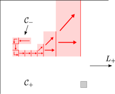
Figure 7. Steps (1) and (2) of the algorithm

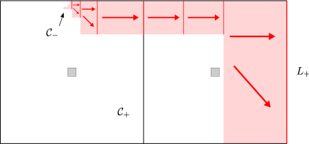
Figure 8. Steps (3)–(5) of the algorithm

We repeat this construction, growing in scale each time, until we are on scale $s_{m}$, then again until we have a block of size $|x-y|/100$, at a distance less than $|x-y|/10$ from $x$. This gives us most of the sequence of blocks with negative index.

We do the same for $y$, getting most of the (reverse) sequence of blocks with positive index, then join the two chains together using Lemmas 5.6 and 5.7. ∎

6. Validity of the Poincaré inequality: the case $\mathbf{a}\in\ell^{2}\setminus\ell^{1}$

In this section we address the case $\mathbf{a}\in\ell^{2}\setminus\ell^{1}$. Our goal (Proposition 6.6) is to prove that in this case the carpet $S_{\mathbf{a}}$ verifies the $p$-Poincaré inequality for each $p>1$.

The overall structure of the proof is similar to that in the previous section. According to Theorems 2.1 and 2.5, it suffices to verify the weighted modulus lower bound (2.1) on the precarpets $S_{\mathbf{a},M}$ with constants independent of $M$. To this end, we construct suitable curve families joining pairs of points in $S_{\mathbf{a},M}$ by concatenating curve families in suitable blocks. The construction of these curve families relies on ‘building block’ lemmas analogous to Lemmas 5.4–5.7 from the previous section. However, the proofs of the ‘building block’ lemmas in the cases $\mathbf{a}\in\ell^{1}$ and $\mathbf{a}\in\ell^{2}\setminus\ell^{1}$ are quite different, and require two completely different methods.

Recall that in the case $\mathbf{a}\in\ell^{1}$, the thinnest part of the carpet has positive length, so we were able to use combinatorial constructions to build modular curve families avoiding all omitted squares in the precarpet $S_{\mathbf{a},M}$.

In the case $\mathbf{a}\in\ell^{2}$, considering only curves which pass through a thin part of the carpet cannot suffice. We instead construct a larger curve family using “bending” machinery which we will develop in subsection 6.2. We use this bending machinery to verify the $p$-Poincaré inequality for $p>1$ via Keith’s theorem 2.1. (This machinery does not apply to the previous case, as the Hölder conjugate exponent $q$ must be finite in order to use Proposition 6.11.)

The bending machinery, and hence our building block lemmas for $p>1$, require the following condition:

(6.1) $$a_{i}<a_{**}\qquad\mbox{for all $i$,}$$

where $a_{**}\in(0,a_{*})$ is a fixed, universal constant whose value is determined in subsection 6.2. Here as always we have $\mathbf{a}=(a_{1},a_{2},\ldots)\in\ell^{2}$.

As before, Theorem 2.2 permits us to reduce to the case that (6.1) holds, because any $S_{\mathbf{a}}$ with $\mathbf{a}\in\ell^{2}$ is the finite union of similar copies of some carpet $S_{\mathbf{a}^{\prime}}$, where $\mathbf{a}^{\prime}\in\ell^{2}$ and all entries of $\mathbf{a}^{\prime}$ are less than $a_{**}$, glued along their boundaries. For the remainder of this section, we impose assumption (6.1).

Fix $p>1$ with Hölder conjugate $q<\infty$. We first define a notion of $q$-connection which generalizes the previous notion of $\infty$-connection. As we will employ bending machinery in this section rather than restricting to paths in the thin part of the carpet, the choice of the distinguished set $\pi_{M}$ is simpler in this setting. For a directed block $(\mathcal{C},L)$ in a square $T^{\prime}$, we let $\pi_{M}(L)=L$ and we let $h$ be the corresponding bijection (which now works out to be the restriction of an affine map).

Definition 6.1.

Suppose that the directed block $(\mathcal{C}_{2},L_{2})$ follows the directed block $(\mathcal{C}_{1},L_{1})$, and let $h\colon\pi_{M}(L_{1})\to\pi_{M}(L_{2})$ be the natural ordered bijection. A path family $\Gamma$ on $\pi_{M}(L_{1})$ in $\mathcal{C}_{2}$ is called an $q$-connection (with constant $C$) if $\gamma(1)=h(\gamma(0))$ for each $\gamma\in\Gamma$, and if $\nu_{\Gamma}\ll\mathcal{H}^{2}{\begin{picture}(12.0,12.0)\put(2.0,0.0){\line(1,0){8.0}} \put(2.0,0.0){\line(0,1){8.0}} \end{picture}\operatorname{spt}(\Gamma)}$ with

(6.2) $$\left\|\frac{d\nu_{\Gamma}}{d\mathcal{H}^{2}}\right\|_{L^{q}(\mathcal{C}_{2};\mathcal{H}^{2})}\leq C\left(\mathcal{H}^{1}(\pi_{M}(L_{1}))\right)^{-1+2/q}.$$

The mysterious exponent on the right hand side of (6.2) can be justified by a dimensional analysis. Note that the measure $\nu_{\Gamma}$ is homogeneous of degree $1$ relative to the scalings $x\mapsto\lambda x$, $\lambda>0$, of $\mathbb{R}^{2}$. Hence the Radon–Nikodym derivative $\tfrac{d\nu_{\Gamma}}{d\mathcal{H}^{2}}$ is homogeneous of degree $-1$. Since the $L^{q}$ norm is computed with respect to Lebesgue measure, it follows that the left hand side of (6.2) is homogeneous of degree $-1+\tfrac{2}{q}$.

In this setting of $\mathbf{a}\in\ell^{2}$, our building block lemmas take the following form. Recall that we fix $0<m\leq M$, and are given directed blocks $(\mathcal{C}_{2},L_{2})$ following $(\mathcal{C}_{1},L_{1})$ in a directed square $(T^{\prime},L^{\prime})\in\mathcal{T}_{m-1}$.

Lemma 6.2 (Expanding).

Suppose that

• $(\mathcal{C}_{1},L_{1})$ and $(\mathcal{C}_{2},L_{2})$ are coherent with $(T^{\prime},L^{\prime})$,

• the sides of $\mathcal{C}_{2}$ perpendicular to $L_{2}$ have length equal to that of $L_{1}$, and

• it holds that $\mathcal{H}^{1}(L_{2})/\mathcal{H}^{1}(L_{1})\leq 10$.

Then there is a $q$-connection $\Gamma$ in $\mathcal{C}_{2}$ with constant $C=C(\|\mathbf{a}\|_{2})$.

Lemma 6.3 (Expanding to the parent generation).

Suppose that

• $(\mathcal{C}_{1},L_{1})$ is coherent with $(T^{\prime},L_{2})$, where $L_{2}=L^{\prime}$,

• the length of $L_{1}$ is equal to the length of an edge of $\mathcal{C}_{2}$ perpendicular to $L_{2}$,

• $L_{1}$ intersects an edge of $T^{\prime}$ perpendicular to $L^{\prime}$, and

• it holds that $\mathcal{H}^{1}(L_{2})/\mathcal{H}^{1}(L_{1})\leq 10$.

Then there is a $q$-connection $\Gamma$ in $\mathcal{C}_{2}$ with constant $C=C(\|\mathbf{a}\|_{2})$.

Lemma 6.4 (Turning).

Suppose that

• $L_{1}$ and $L_{2}$ are perpendicular, and

• all edges of $\mathcal{C}_{2}$ have length equal to the length of $L_{1}$.

Then there is a $q$-connection $\Gamma$ in $\mathcal{C}_{2}$ with constant $C=C(\|\mathbf{a}\|_{2})$.

Lemma 6.5 (Going straight).

Suppose that

• $(\mathcal{C}_{1},L_{1})$ and $(\mathcal{C}_{2},L_{2})$ are coherent with $(T^{\prime},L^{\prime})$,

• $L_{1}$ and $L_{2}$ are of equal length, and

• the sides of $\mathcal{C}_{2}$ perpendicular to $L_{2}$ have length in $[\mathcal{H}^{1}(L_{1})/2,10\mathcal{H}^{1}(L_{1})]$.

Then there is a $q$-connection $\Gamma$ in $\mathcal{C}_{2}$ with constant $C=C(\|\mathbf{a}\|_{2})$.

To produce the desired $q$-connection in these lemmas, we will use the bending machinery which we develop in subsection 6.2. We therefore postpone the proof of these lemmas until that time. Assuming for the moment their validity, we complete the proof of the $p$-Poincaré inequality.

6.1. Verification of the $p$-Poincaré inequality for $p>1$

We prove the following proposition.

Proposition 6.6.

Suppose that $\mathbf{a}\in\ell^{2}$ and $p>1$. Then $S_{\mathbf{a}}$ admits a $p$-Poincaré inequality.

Proof.

This proof is virtually identical to that of Proposition 5.8, using the new building block lemmas 6.2–6.5. Lemma 5.9 remains the same, except that condition (4) is replaced by

1. For each $i=(K_{-}+1),\ldots,-1$, $(\mathcal{C}_{i},L_{i})$ follows $(\mathcal{C}_{i-1},L_{i-1})$; for each $i=1,\ldots,K_{+}-1$, $(\mathcal{C}_{i},L_{i})$ follows $(\mathcal{C}_{i+1},L_{i+1})$; $(\mathcal{C}_{0},L_{1})$ follows $(\mathcal{C}_{-1},L_{-1})$, and $(\mathcal{C}_{0},L_{-1})$ follows $(\mathcal{C}_{1},L_{1})$. In each case, $\Gamma_{i}$ is a $q$-connection with constant $C_{0}$.

This condition follows by using Lemmas 6.2–6.5 and exactly the same argument as before.

We now complete the proof of Proposition 6.6. First, concatenate the path families $\Gamma_{K_{-}},\ldots,\Gamma_{K_{+}}$ by gluing paths using the natural ordered bijection on each block. This gives a path family $\Gamma$ consisting of pairwise disjoint, rectifiable curves joining $x$ to $y$, carrying a probability measure $\sigma=\sigma_{\Gamma}$ on $\Gamma$ which agrees with $\sigma_{\Gamma_{i}}$ for each $i$ on $\mathcal{C}_{i}$. The measure $\nu=\nu_{\Gamma}$ on the support of $\Gamma$ defined as in (5.4) restricts to $\nu_{\Gamma_{i}}$ on each $\mathcal{C}_{i}$, and is absolutely continuous with respect to $\mu_{xy}$. For $i={K_{-}},\ldots,{K_{+}}$, we have the following bound on the Radon–Nikodym derivative $\frac{d\nu}{d\mu_{xy}}$:

$$\left\|\frac{d\nu}{d\mu_{xy}}\right\|_{L^{q}(\mathcal{C}_{i};\mu_{xy})} \asymp\left\|\frac{d\nu}{d\mathcal{H}^{2}}\right\|_{L^{q}(\mathcal{C}_{i};\mathcal{H}^{2})}\operatorname{diam}(\mathcal{C}_{i})^{1-1/q}$$

$$\lesssim\left(\mathcal{H}^{1}(\pi_{M}(L_{i}))\right)^{-1+2/q}\operatorname{diam}(\mathcal{C}_{i})^{1-1/q}$$

$$\lesssim\operatorname{diam}(\mathcal{C}_{i})^{-1+2/q}\operatorname{diam}(\mathcal{C}_{i})^{1-1/q}=\operatorname{diam}(\mathcal{C}_{i})^{1/q}.$$

This bound also holds on $\mathcal{C}_{K_{-}}$ and $\mathcal{C}_{K_{+}}$: note that on $\operatorname{spt}(\Gamma_{K_{-}})\subset\mathcal{C}_{K_{-}}$, both $\nu$ and $\mu_{xy}$ are comparable to the measure $A\mapsto\int_{A}1/|x-z|\ d\mathcal{H}^{2}(z)$. An elementary calculation gives

$$\left\|\frac{d\nu}{d\mu_{xy}}\right\|_{L^{q}(\mathcal{C}_{K_{-}};\mu_{xy})}\lesssim s_{M}^{1/q}\asymp\operatorname{diam}(\mathcal{C}_{K_{-}})^{1/q}.$$

An analogous argument proves the bound for $\mathcal{C}_{K_{+}}$. Summing over $i$ gives

$$\left\|\frac{d\nu}{d\mu_{xy}}\right\|_{L^{q}(\mu_{xy})}^{q}=\sum_{i={K_{-}}}^{K_{+}}\left\|\frac{d\nu}{d\mu_{xy}}\right\|_{L^{q}(\mathcal{C}_{i},\mu_{xy})}^{q}\lesssim\sum_{i={K_{-}}}^{K_{+}}\operatorname{diam}(\mathcal{C}_{i})\lesssim|x-y|.$$

If $\rho$ is admissible for $\Gamma$, then

$$1 \leq\int_{\Gamma}\int_{\gamma}\rho\,ds\,d\sigma(\gamma)=\int_{\operatorname{spt}\Gamma}\rho\ d\nu$$

$$=\int_{S_{\mathbf{a},M}}\rho\,\frac{d\nu}{d\mu_{xy}}\,d\mu_{xy}\leq\|\rho\|_{L^{p}(\mu_{xy})}\ \left\|\frac{d\nu}{d\mu_{xy}}\right\|_{L^{q}(\mu_{xy})}\lesssim\|\rho\|_{L^{p}(\mu_{xy})}\ |x-y|^{1/q}.$$

Consequently

$$\int_{S_{\mathbf{a},M}}\rho^{p}\,d\mu_{xy}\gtrsim|x-y|^{-p/q}=|x-y|^{1-p}$$

and so (2.1) holds. This completes the proof of Proposition 6.6, modulo the building block lemmas 6.2–6.5. ∎

6.2. Bending curve families

In this section, we introduce the bending machinery needed to prove Lemmas 6.2–6.5. The methods used allow us to build curve families of positive modulus in a wide class of compact planar sets, as illustrated by the following theorem, which gives a general sufficient condition for such curve families.

Theorem 6.7.

Let $D\subset\mathbb{R}^{2}$ be the closure of a domain and let $\mathbf{a}=(a_{1},a_{2},\ldots)\in\ell^{2}$ with $a_{m}\in(0,1)$ for all $m$. For each $m$, let $s_{m}=\prod_{j=1}^{m}a_{j}$, and let $\mathcal{U}_{m}$ be a family of disjoint open subsets of $D$. Assume that the following two conditions are satisfied:

• for all $U\in\mathcal{U}_{m}$, $\operatorname{diam}U\leq 2s_{m}$, and

• for all $U\in\mathcal{U}_{m}$ and all $V\in\{\partial D\}\cup\mathcal{U}_{1}\cup\mathcal{U}_{2}\cup\cdots\cup\mathcal{U}_{m}$ with $V\neq U$, we have $\operatorname{dist}(U,V)\geq\tfrac{2}{5}s_{m-1}$.

Let $S_{M}:=D\setminus\cup\{U:U\in\mathcal{U}_{1}\cup\cdots\cup\mathcal{U}_{M}\}$ and

$$S=\bigcap_{M\geq 0}S_{M}.$$

Then for all $p>1$ and all relatively open balls $B\subset S$, there exists a curve family contained in $B$ with positive $p$-modulus with respect to the measure $\mathcal{H}^{2}$ restricted to $S$.

The coefficients $2$ and $\tfrac{2}{5}$ in Theorem 6.7 have been fixed for the sake of definiteness and can be varied without changing the result.

In the setting of the carpets $S_{\mathbf{a}}$, our arguments give the following corollary, independent of Theorem 1.6.

Corollary 6.8.

For any $p>1$ and $\mathbf{a}\in\ell^{2}$, there exists a positive constant $C=C(p,\mathbf{a})$ so that the $p$-modulus of the curve family joining the left hand edge to the right hand edge of $S_{\mathbf{a}}$ is at least $C$. If $\mathbf{a}$ is monotone decreasing, then $C=C(p,\|\mathbf{a}\|_{2})$.

The basic idea of the construction in this section is as follows. We present an algorithm which accepts as input a family of curves in the plane and which yields as output a new family of curves which avoids a prespecified obstacle at a small quantitative multiplicative cost to the $p$-modulus. We apply this algorithm recursively to avoid all of the omitted sets. The algorithm in question works by splitting the family of input curves in two pieces which are deformed to pass on either side of the obstacle. (Similar ideas appear in a paper of Chris Bishop [1] on $A_{1}$ deformations of the plane.)

The curve families that we consider are axiomatized in the following definition.

Definition 6.9.

An open measured family of $C^{2}$ curves is a collection $\Gamma$ of disjoint, oriented $C^{2}$ curves in a set $X\subset\mathbb{R}^{2}$, together with a probability measure $\sigma$ on $\Gamma$, such that the union of all the curves in $\Gamma$, denoted $\operatorname{spt}\Gamma$, is an open subset of $X$. We will denote such a pair by $(\Gamma,\sigma)$, or just by $\Gamma$ if the measure $\sigma$ is understood.

There is a natural measure $\nu_{\Gamma}=\nu_{(\Gamma,\sigma)}$ defined on $\operatorname{spt}\Gamma$ by

(6.3) $$\nu_{\Gamma}(V)=\int_{\Gamma}\mathcal{H}^{1}(V\cap\gamma)d\sigma(\gamma).$$

At this point, the integral in (6.3) should be interpreted as an upper integral with value in $[0,\infty]$. However, under the conditions of Definition 6.10, $\nu_{\Gamma}$ will be a finite Borel measure.

We assume that each curve in $\Gamma$ is parameterized with nonzero speed, consistent with the specified orientation. Since each curve in $\Gamma$ is $C^{2}$, there is a vector field $\dot{\Gamma}$ defined on $\operatorname{spt}\Gamma$ such that $\dot{\Gamma}(x)$ coincides with the unit tangent vector to the unique curve $\gamma_{x}\in\Gamma$ passing through $x$ at time $t_{x}$. In fact,

(6.4) $$\dot{\Gamma}(x)=\frac{\gamma_{x}^{\prime}(t_{x})}{|\gamma_{x}^{\prime}(t_{x})|}.$$

Definition 6.10.

Fix $\delta_{0}\geq 0$ and $r_{0}>0$. Suppose $(\Gamma,\sigma)$ is an open measured family of $C^{2}$ curves, with $\nu_{\Gamma}$ defined as in (6.3). We say that $(\Gamma,\sigma)$ is a $\delta_{0}$-good family of curves on scales less than $r_{0}$ if for any ball $B(z,r)$, $z\in X$, $0<r\leq r_{0}$ we have the following properties:

• If $B(z,r)$ does not contain any endpoint of any $\gamma\in\Gamma$, then the complement of the closure of $\operatorname{spt}\Gamma$ in $B(z,r)$ is a connected open set.

• For any $x,y\in B(z,r)$,

  $$\angle(\dot{\Gamma}(x),\dot{\Gamma}(y))\leq\delta_{0}\left(\frac{|x-y|}{2r_{0}}\right)^{2/3},$$

  where $\angle(\mathbf{v},\mathbf{w})$ denotes the angle between vectors $\mathbf{v}$ and $\mathbf{w}$.

• There is a constant $A_{z,r}\in(0,\infty)$ so that on $B(z,r)\cap\operatorname{spt}\Gamma$ the Radon-Nikodym derivative $w_{\Gamma}=d\nu_{\Gamma}/d\mathcal{H}^{2}$ exists, is $\frac{2}{3}$-Hölder continuous with constant $(2r_{0})^{-2/3}A_{z,r}\delta_{0}$, and satisfies

  $$w_{\Gamma}(B(z,r)\cap\operatorname{spt}\Gamma)\subset[(1+\delta_{0})^{-1}A_{z,r},(1+\delta_{0})A_{z,r}].$$

The first condition ensures that $\overline{\operatorname{spt}\Gamma}\cap B(z,r)$ is either the empty set, one half of the ball, all of the ball except for one open gap, or all of the ball. Figure 9 illustrates typical instances of this.

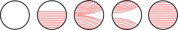
Figure 9. Structure of $\overline{\operatorname{spt}\Gamma}\cap B(z,r)$

The last two conditions guarantee that the vector field $\dot{\Gamma}$ is $\frac{2}{3}$-Hölder continuous (with suitable constant) and that the Radon-Nikodym derivative $w_{\Gamma}=\tfrac{d\nu_{\Gamma}}{d\mathcal{H}^{2}}$ exists and is locally close to constant on $\operatorname{spt}\Gamma$.

Why are the vector fields only Hölder continuous? If they were Lipschitz continuous, then by the uniqueness of solutions to ODE with Lipschitz coefficients, the curves could not split to bend round an obstacle. The choice of $\frac{2}{3}$ is fixed in view of the cubic spline which we construct in Lemma 6.13(4). This choice is merely a convenience; any Hölder exponent strictly less than one would serve our purposes equally well.

The following proposition provides the key inductive step in bending curve families with control on their modulus. We postpone its proof until subsection 6.4.

Proposition 6.11.

For any sufficiently small $\delta_{0}>0$, there exist positive constants $a^{\prime}$ and $C$ with the following property.

Suppose $(\Gamma_{i},\sigma_{i})$ is a $\delta_{0}$-good family of curves on scales smaller than $s_{i}$ in $\mathbb{R}^{2}$, for some $s_{i}>0$, and we are given $a_{i+1}\in(0,a^{\prime}]$. Let $\nu_{i}=\nu_{\Gamma_{i}}$ be the natural measure, let $w_{i}=d\nu_{i}/d\mathcal{H}^{2}$ be the corresponding weight, and set $s_{i+1}=a_{i+1}s_{i}$. Then given any $z\in\operatorname{spt}\Gamma_{i}$, with no curves in $\Gamma_{i}$ stopping inside $B(z,s_{i})$, we can deform $(\Gamma_{i},\sigma_{i})$ inside $B(z,s_{i}/5)$ into a new open measured curve family $(\Gamma_{i+1},\sigma_{i+1})$ that is $\delta_{0}$-good on scales smaller than $s_{i+1}$, so that $\operatorname{spt}\Gamma_{i+1}$ does not meet $B(z,2s_{i+1})$ and

(6.5) $$\int_{B(z,s_{i}/5)}|w_{i+1}|^{q}d\mathcal{H}^{2}\leq(1+Ca_{i+1}^{2})\int_{B(z,s_{i}/5)}|w_{i}|^{q}d\mathcal{H}^{2}.$$

By “deform”, we mean that there exists a $C^{2}$ homeomorphism of the plane which restricts to the identity outside $B(z,s_{i}/5)$, and, up to discarding finitely many curves, induces a well defined, measure preserving bijection between $(\Gamma_{i},\sigma_{i})$ and $(\Gamma_{i+1},\sigma_{i+1})$. We emphasize that the numbers $s_{i}>0$ and $a_{i+1}\in(0,a^{\prime}]$ in the statement of Proposition 6.11 are arbitrary and are not assumed to be arising from a specific sequence $\mathbf{a}$ under consideration.

Intuitively, Proposition 6.11 asserts that we can deform $\Gamma_{i}$ inside a ball $B$ on a given scale $s_{i}$ so as to avoid a prespecified obstacle of size $s_{i+1}$ (in this case, a ball of radius $2s_{i+1}$ concentric with $B$) and so that the $\ell^{q}$ norm of the associated weight increases multiplicatively by at most a factor of $1+Ca_{i+1}^{2}$, where $C$ is independent of $\mathbf{a}$. The point is that we can repeatedly apply the proposition (on smaller and smaller scales) without losing control of $\delta_{0}$.

6.3. Using the bending machinery

We now prove our building block lemmas, Theorem 6.7 and Corollary 6.8.

Proof of Lemmas 6.2–6.5.

Recall that $(\mathcal{C}_{2},L_{2})$ is a directed block following $(\mathcal{C}_{1},L_{1})$ in a directed square $(T^{\prime},L^{\prime})\in\mathcal{T}_{m-1}$. Let $\Gamma_{m}$ be the open, measured curve family consisting of straight line segments in $\mathbb{R}^{2}$ connecting each point of the interior of $L_{1}$ to the corresponding point of $L_{2}$ under the natural ordered bijection, equipped with the measure $\sigma_{m}$ induced from normalized linear measure on $L_{1}$. See Figure 10.

\psfrag{C1}{$\mathcal{C}_{1}$}\psfrag{C2}{$\mathcal{C}_{2}$}\psfrag{L1}{$L_{1}$}\psfrag{L2}{$L_{2}$}\includegraphics[width=93.94955pt]{pExpand.eps}

\psfrag{C1}{$\mathcal{C}_{1}$}\psfrag{C2}{$\mathcal{C}_{2}$}\psfrag{L1}{$L_{1}$}\psfrag{L2}{$L_{2}$}\includegraphics[width=93.94955pt]{pNextGen.eps}

\psfrag{C1}{$\mathcal{C}_{1}$}\psfrag{C2}{$\mathcal{C}_{2}$}\psfrag{L1}{$L_{1}$}\psfrag{L2}{$L_{2}$}\includegraphics[width=93.94955pt]{pTurning.eps}

\psfrag{C1}{$\mathcal{C}_{1}$}\psfrag{C2}{$\mathcal{C}_{2}$}\psfrag{L1}{$L_{1}$}\psfrag{L2}{$L_{2}$}\includegraphics[width=93.94955pt]{pStraight.eps}

Figure 10. Initial curve families for the $p>1$ case of Lemmas 5.4 - 5.7

Let $w_{m}=d\nu_{\Gamma_{m}}/d\mathcal{H}^{2}$ be the natural weight function associated to $\Gamma_{m}$. Observe that on $\operatorname{spt}\Gamma_{m}$, we have $\nu_{\Gamma_{m}}\asymp\mathcal{H}^{1}(\pi_{M}(L_{1}))^{-1}\mathcal{H}^{2}$, and that $\mathcal{H}^{2}(\operatorname{spt}\Gamma_{m})\asymp(\mathcal{H}^{1}(\pi_{M}(L_{1})))^{2}$, so

(6.6) $$\|w_{m}\|_{q}\asymp(\mathcal{H}^{1}(\pi_{M}(L_{1})))^{-1+2/q}.$$

Since a $q$-connection must lie in $\mathcal{C}_{2}\cap S_{\mathbf{a},M}$, we ‘bend’ this initial family around the subsquares of $\mathcal{C}_{2}$ that were removed in the construction of $S_{\mathbf{a},M}$. This construction is inductive, building open measured curve families $(\Gamma_{i},\sigma_{i})$ for $m\leq i\leq M$.

Observe that there exists a universal constant $\delta_{1}>1$ so that any such initial curve family $\Gamma_{m}$ is a $\delta_{1}$-good curve family on scales below $s_{m}$. We use the following sublemma.

Sublemma 6.12.

For any $\epsilon\in(0,1)$, a $\delta_{1}$-good curve family on scales below $r_{1}$ is also a $(\delta_{1}\epsilon^{1/3})$-good curve family on scales below $\epsilon r_{1}$.

Proof.

The only non-trivial estimate is the last part of Definition 6.10(((6.10))). On a ball of radius $\epsilon r_{1}$, with associated constant $A$, the ratio of maximum to minimum values of $w$ is at most

$$\frac{(1+\delta_{1})^{-1}A+(2r_{1})^{-2/3}A\delta_{1}(2\epsilon r_{1})^{2/3}}{(1+\delta_{1})^{-1}A}\leq 1+(1+\delta_{1})\delta_{1}\epsilon^{2/3}\leq(1+\delta_{1}\epsilon^{1/3})^{2}.\qed$$

Fix the constant $a_{**}$ in (6.1) so that

$$a_{**}=a^{\prime}\delta_{1}^{-3}\delta_{0}^{3}\leq a^{\prime},$$

where $\delta_{0}$ and $a^{\prime}$ are chosen by Proposition 6.11. The sublemma above shows that $\Gamma_{m}$ is a $\delta_{0}$-good curve family on scales below $s_{m}^{\prime}:=\delta_{1}^{-3}\delta_{0}^{3}s_{m}$.

The removed squares of side $s_{m+1}$ in $\mathcal{C}_{2}$ are all at least $s_{m}/2$ apart, so we apply Proposition 6.11 to $(\Gamma_{m},\sigma_{m})$ independently for some $z$ in each such removed square, with values $s_{i}=s_{m}^{\prime}$ and $s_{i+1}=s_{m+1}$; this is valid since $s_{m+1}/s_{m}^{\prime}<a^{\prime}$. Denote the resulting open, measured curve family by $(\Gamma_{m+1},\sigma_{m+1})$, which is $\delta_{0}$-good on scales below $s_{m+1}$.

By applying (6.5) around each removed square, we have that the natural weight function $w_{m+1}$ associated to $\Gamma_{m+1}$ satisfies

(6.7) $$\|w_{m+1}\|_{q}\leq(1+Ca_{m+1}^{2})^{1/q}\|w_{m}\|_{q}.$$

Similarly, for $i=m+1,\ldots,M-1$, we build $(\Gamma_{i+1},\sigma_{i+1})$ from $(\Gamma_{i},\sigma_{i})$ by applying Proposition 6.11 indepenently for each removed square of side $s_{i+1}$; this is valid since $s_{i+1}/s_{i}=a_{i+1}\leq a_{**}<a^{\prime}$. We obtain a open, measured curve family $(\Gamma,\sigma)=(\Gamma_{M},\sigma_{M})$, with $\operatorname{spt}\Gamma$ in $\mathcal{C}_{2}\cap S_{\mathbf{a},M}$. Iterating the weight bound of (6.7), we see that

$$\left\|\frac{d\nu_{\Gamma}}{d\mathcal{H}^{2}}\right\|_{L^{q}(\mathcal{C}_{2},\mathcal{H}^{2})}=\|w_{M}\|_{q}\leq\left(\prod_{i=m+1}^{M}(1+Ca_{i}^{2})\right)^{1/q}\|w_{m}\|_{q}\leq\exp\left(\frac{C}{q}||\mathbf{a}||_{2}^{2}\right)\mathcal{H}^{1}(\pi_{M}(L_{1}))^{-1+2/q},$$

where this last inequality uses (6.6). This implies that the output family is a $q$-connection. ∎

A similar argument extends to give modulus bounds.

Proof of Theorem 6.7.

We fix $a^{\prime}<\frac{1}{100}$, $\delta_{0}$, and $C$ as in Proposition 6.11 and choose $M$ so that $a_{i}<a^{\prime}$ when $i\geq M$. Note that if $\mathbf{a}$ is monotone decreasing, then $M$ depends only on $\|\mathbf{a}\|_{2}$.

If $S$ has nonempty interior we are done, since open sets in $\mathbb{R}^{2}$ certainly contain curve families with positive $p$-modulus. Otherwise there exists $\mathcal{U}_{M^{\prime}}\neq\emptyset$, for some $M^{\prime}\geq M$. Choose $U\in\mathcal{U}_{M^{\prime}}$ so that $\operatorname{dist}(U,\partial D)\geq\frac{2}{5}s_{M^{\prime}-1}\geq 10s_{M^{\prime}}$. We choose a square $W\subset D$ of side $s_{M^{\prime}}$ so that $\operatorname{dist}(W,U)$ is between $2s_{M^{\prime}}$ and $3s_{M^{\prime}}$. By the assumptions of the theorem, and choice of $M$, $W$ only meets sets from $\cup_{m\geq(M^{\prime}+1)}\mathcal{U}_{m}$, which have diameter much smaller than $W$.

We choose coordinates so that $W=[0,s_{M^{\prime}}]^{2}$. Let $\Gamma_{M^{\prime}}$ be the family of curves $\{\gamma_{u}:u\in(0,s_{M^{\prime}})\}$, where $\gamma_{u}:(0,s_{M^{\prime}})\rightarrow W$ is defined as $\gamma_{u}(t)=(t,u)$. We equip $\Gamma_{M^{\prime}}$ with the probability measure $\sigma_{M^{\prime}}$ given by scaling Lebesgue measure on $(0,s_{M^{\prime}})$ by $s_{M^{\prime}}^{-1}$. Observe that $\Gamma_{M^{\prime}}$ is a $0$-good family of curves on scales below $s_{M^{\prime}}$, with $w_{M^{\prime}}\equiv s_{M^{\prime}}^{-1}$.

We now build measured curve families $(\Gamma_{m},\sigma_{m})$ for $m\geq M^{\prime}$ that are $\delta_{0}$-good on scales below $s_{m}$, with the additional property that

(6.8) $$\operatorname{spt}\Gamma_{m}\cap\big{(}[s_{M^{\prime}}/4,3s_{M^{\prime}}/4]\times\mathbb{R}\big{)}\subset S_{m}.$$

Let $\nu_{m}=\nu_{\Gamma_{m}}$ be the natural measure on $\operatorname{spt}\Gamma_{m}$ and let $w_{m}=d\nu_{m}/d\mathcal{H}^{2}$ be the corresponding weight.

The construction is inductive. Assume that we have constructed a measured curve family $(\Gamma_{m},\sigma_{m})$ that is $\delta_{0}$-good on scales below $s_{m}$. We apply Proposition 6.11 to bend $\Gamma_{m}$ around each set $V\in\mathcal{U}_{m+1}$ which meets $[s_{M^{\prime}}/8,7s_{M^{\prime}}/8]\times[-s_{M^{\prime}},2s_{M^{\prime}}]$. As the sets in $\mathcal{U}_{m+1}$ are all at least $s_{m}$ apart, we can apply Proposition 6.11 at each location independently to create a new measured curve family $(\Gamma_{m+1},\sigma_{m+1})$, which is $\delta_{0}$-good on scales below $s_{m+1}$. (Proposition 6.11 requires that no curve ends near where we bend; this is why we restrict the obstacles that we bend around.) These curve families satisfy (6.8) for $m\geq M^{\prime}$.

As in the proof of Lemmas 6.2–6.5, we conclude that for all $m\geq M^{\prime}$ the natural weight function $w_{m}$ associated to $\Gamma_{m}$ satisfies

(6.9) $$\|w_{m}\|_{q}\leq\left(\prod_{i=M^{\prime}+1}^{\infty}(1+Ca_{i}^{2})\right)^{1/q}\|w_{M^{\prime}}\|_{q}\leq\exp\left(\frac{C}{q}||\mathbf{a}||_{2}^{2}\right)\|w_{M^{\prime}}\|_{q}$$

If $\rho:B\rightarrow[0,\infty]$ is admissible for $\operatorname{mod}_{p}\,\Gamma_{m}$, that is, $1\leq\int_{\gamma}\rho\,d\mathcal{H}^{1}$ for each $\gamma\in\Gamma_{m}$, then by averaging over $\Gamma_{m}$ with respect to $\sigma_{m}$, we see that

(6.10) $$\begin{split}1\leq\int_{\Gamma_{m}}\int_{\gamma}\rho\ d\mathcal{H}^{1}d\sigma_{m}(\gamma)=\int_{\operatorname{spt}\Gamma_{m}}\rho\ d\nu_{m}=\int_{\operatorname{spt}\Gamma_{m}}\rho\,w_{m}\ d\mathcal{H}^{2}\leq\|\rho\|_{p}\ \|w_{m}\|_{q},\end{split}$$

where $\frac{1}{p}+\frac{1}{q}=1$. Combining (6.9), (6.10) and $\mathbf{a}\in\ell^{2}$, we see that $\operatorname{mod}_{p}\,\Gamma_{m}$ is uniformly bounded from below independent of $m$.

Each curve $\gamma\in\Gamma_{m}$ has a subcurve $\gamma^{\prime}$ which joins the set $\{s_{M^{\prime}}/4\}\times\mathbb{R}$ to $\{3s_{M^{\prime}}/4\}\times\mathbb{R}$, and $\gamma^{\prime}\subset S_{m}$. Let $\Gamma_{m}^{\prime}$ be the collection of all such curves. By basic properties of the modulus, $\operatorname{mod}_{p}\,\Gamma_{m}^{\prime}\geq\operatorname{mod}_{p}\,\Gamma_{m}$.

Thus for every $m\geq M^{\prime}$, there is a curve family $\Gamma_{m}^{\prime}$ in $S_{m}$ with $p$-modulus bounded from below independent of $m$. By the upper semicontinuity of modulus (see, for instance, Heinonen–Koskela [19, §3] or Keith [22, Theorem 1]), this bound will continue to the limit. ∎

Proof of Corollary 6.8.

Again, choose $a^{\prime}$ as in Proposition 6.11 and choose $M$ so that $a_{i}<a^{\prime}$ when $i\geq M$. The $p$-modulus of the family of curves joining the left and right edges of the carpet $S_{\mathbf{a}}$ is bounded from below by the $p$-modulus of the family of curves $\Gamma$ joining the left and right edges of the strip $([0,1]\times[0,s_{M}])\cap S_{\mathbf{a}}$.

Let $\Gamma_{M}$ be the family of horizontal lines in $T=[0,1]\times[0,s_{M}]$, with induced natural weight $w_{M}$, equal to $s_{M}^{-1}$ on $T$, and so having $\|w_{M}\|_{q}=s_{M}^{-1/p}$. The argument in the proof of Theorem 6.7, in particular (6.9) and (6.10), give that any admissible function $\rho$ for $\Gamma$ satisfies

$$1\leq\|\rho\|_{p}\exp\left(\frac{C}{q}\|\mathbf{a}\|_{2}^{2}\right)\|w_{M}\|_{q}.$$

Therefore, as $\|w_{M}\|_{q}\leq C(\mathbf{a})<\infty$, we have $\operatorname{mod}_{p}(\Gamma)>0$. Finally, we note that in the case when $\mathbf{a}$ is monotone decreasing, then $M$ can be chosen only depending on $||\mathbf{a}||_{2}$ (and not on the actual sequence $\mathbf{a}$). This implies that $\|w_{M}\|_{q}\leq C(\|\mathbf{a}\|_{2})$, and this establishes the final claim of the corollary. ∎

It remains to establish Proposition 6.11. This is the goal of the following subsection. The argument is rather technical although essentially elementary. The reader is invited to skip the remainder of this section on a first reading of the paper.

6.4. Compressing curve families: the proof of Proposition 6.11

The following construction is standard. For the convenience of the reader we provide a short proof.

Lemma 6.13.

There is a $C^{2}$ function $\varphi:[-1,1]\rightarrow[0,1]$ which satisfies

1. $\varphi|_{[-0.1,0.1]}\equiv 1$,

2. the support of $\varphi$ lies in $[-0.9,0.9]$,

3. $|\varphi^{\prime}|\leq 5/2$, $|\varphi^{\prime\prime}|\leq 25/2$, and

4. $|\varphi^{\prime}|\leq 14\varphi^{2/3}$.

Proof.

Choose $\varphi^{\prime\prime}:[-1,1]\rightarrow\mathbb{R}$ to be the simplest piecewise linear function whose graph passes through the points $(\pm 1,0)$, $(\pm 0.9,0)$, $(\pm 0.7,b)$, $(\pm 0.3,-b)$, $(\pm 0.1,0)$, and $(0,0)$, where $b>0$ is a constant to be determined.

Assuming that $\varphi^{\prime}(-1)=\varphi(-1)=0$, we integrate to find $\varphi$. Note that $\varphi|_{[-0.1,0.1]}\equiv 0.08b$, so we choose $b=1/0.08=25/2$. With this choice, $|\varphi^{\prime}|\leq 0.2b=5/2$ and $|\varphi^{\prime\prime}|\leq b=25/2$. Hence conditions (1), (2) and (3) are satisfied.

Finally, note that for $0\leq h\leq 0.2$, $\varphi^{\prime\prime}(-0.9+h)=5bh=\frac{125}{2}h$, $\varphi^{\prime}(-0.9+h)=\frac{5}{2}bh^{2}=\frac{125}{4}h^{2}$ and $\varphi(-0.9+h)=\frac{5}{6}bh^{3}=\frac{125}{12}h^{3}$, so

$$|\varphi^{\prime}(-0.9+h)|=5\left(\frac{3}{2}\right)^{2/3}|\varphi(-0.9+h)|^{2/3}\leq 10|\varphi(-0.9+h)|^{2/3}.$$

This bound also applies for $x\in[0.7,0.9]$. On the other hand, for $x\in[-0.7,0.7]$ we have $\varphi(x)\geq\varphi(-0.7)=\frac{1}{12}$ and $|\varphi^{\prime}(x)|\leq\frac{5}{2}$, so $|\varphi^{\prime}(x)|\leq\frac{5}{2}=\frac{5}{2}\cdot 12^{2/3}\left(\frac{1}{12}\right)^{2/3}\leq 14|\varphi(x)|^{2/3}$. ∎

We now begin the proof of Proposition 6.11.

Proof of Proposition 6.11.

We fix a positive constant $\delta_{0}\leq\tfrac{1}{200}$. We will choose a large positive integer $N=N(\delta_{0})\geq 5$; the precise choice will be made later in the proof. Finally, we assume that $a^{\prime}\leq 10^{-2-N}$; we only consider $a_{i}<a^{\prime}$.

Let $(\Gamma_{i},\sigma_{i})$ be a $\delta_{0}$-good family of curves on scales smaller than $s_{i}$, let $\nu_{i}$ be the corresponding measure as defined in (6.3), and suppose that $z\in\operatorname{spt}\Gamma_{i}$. We can apply an isometry of $\mathbb{R}^{2}$ to reduce to the case when $z=0$,

$$B(z,2s_{i+1}) \subset P:=[-2s_{i+1},2s_{i+1}]^{2}$$

$$\subset Q:=[-10^{N}s_{i+1},10^{N}s_{i+1}]^{2}$$

$$\subset R:=[-s_{i}/10,s_{i}/10]^{2}\subset B(z,s_{i}/5),$$

and $\dot{\Gamma_{i}}(0)$ has horizontal slope. This last assertion, in conjunction with Definition 6.10((6.10)), implies that all curves in $R$ have slopes within $(1/5)\delta_{0}$ of zero. In particular, each curve $\gamma\in\Gamma_{i}$ is a graph over the $x$-axis inside $R$. Henceforth we will assume that each curve is given in graph form: $y=\gamma(x)$. Nevertheless, we continue to denote by $\gamma=\{(x,\gamma(x))\}$ the graph itself.

We choose a curve $\gamma_{0}$ which passes near $P$ and either bounds an existing gap in $Q$, or is far from an existing gap in $Q$. To be precise, let $U$ be the complement of $\overline{\operatorname{spt}\Gamma_{i}}$ in $B(z,s_{i}/5)$ which, by condition (6.10), is a connected open set. Moreover, $\partial_{\infty}U\cap B(z,s_{i}/5)$ lies in one or two $C^{2}$ curves whose slopes satisfy, along with $\Gamma_{i}$, condition ((6.10)). If $U$ meets $L=\{0\}\times[-3s_{i+1},3s_{i+1}]$, choose $\gamma_{0}$ which bounds an edge of $U$ meeting $L$ (as $(0,0)\notin U$, such a $\gamma_{0}$ exists). If $U$ does not meet $L$, choose $\gamma_{0}\in\Gamma_{i}$ which passes through $(0,-3s_{i+1})$ or $(0,3s_{i+1})$, chosen so that

(6.11) $$\operatorname{dist}(\gamma_{0}(0),U)\geq 5s_{i+1}.$$

(Recall that $\gamma_{0}$ is a graph over the $x$-axis and we have normalized so that $z=0$.)

We will compress the curves inside $Q$ into the complement of $P$, leaving everything unchanged in $R\setminus Q$. To build $\Gamma_{i+1}$ we will delete $\gamma_{0}$ from $\Gamma_{i}$ if necessary, and apply a diffeomorphism on $X\setminus\gamma_{0}$ to compress the remaining curves around $P$. The two options in the choice of $\gamma_{0}$ correspond to either enlarging an existing gap in $\Gamma_{i}$, or creating a new gap at least $4s_{i+1}$ from any previous gap.

We rescale the function $\varphi$ from Lemma 6.13 to the scale of $Q$ by defining

$$\tilde{\varphi}(x)=6s_{i+1}\varphi\left(\frac{x}{10^{N}s_{i+1}}\right).$$

Note that $|\tilde{\varphi}^{\prime}|\leq 10^{2-N}$, $|\tilde{\varphi}^{\prime\prime}|\leq 10^{2-2N}s_{i+1}^{-1}$, and

(6.12) $$|\tilde{\varphi}^{\prime}|\leq 10^{2-N}\left(\frac{\tilde{\varphi}}{2s_{i+1}}\right)^{2/3}.$$

We now define the local compression map $H:Q\setminus\{\gamma_{0}\}\rightarrow Q$. Let $g:Q\setminus\{\gamma_{0}\}\rightarrow[-1,1]$ be given by

$$g(x,y)=\begin{cases}\varphi\left(\frac{y-\gamma_{0}(x)}{10^{N}s_{i+1}-\gamma_{0}(x)}\right)&\text{if }y\in(\gamma_{0}(x),10^{N}s_{i+1})\\ -\varphi\left(\frac{\gamma_{0}(x)-y}{10^{N}s_{i+1}+\gamma_{0}(x)}\right)&\text{if }y\in(-10^{N}s_{i+1},\gamma_{0}(x)).\end{cases}$$

Since the functions $\gamma_{0}$ and $\varphi$ are $C^{2}$ and $10^{N}s_{i+1}-\gamma_{0}$ and $10^{N}s_{i+1}+\gamma_{0}$ take values in $[0.99\cdot 10^{N}s_{i+1},1.01\cdot 10^{N}s_{i+1}]$, $g$ is $C^{2}$. The function $g$ varies from $0$ near the top of $Q$ to $1$ just above $\gamma_{0}$, and from $-1$ just below $\gamma_{0}$ to $0$ near the bottom of $Q$. Next let

$$h(x,y)=y+\tilde{\varphi}(x)\cdot g(x,y),$$

and define

$$H(x,y)=\big{(}x,h(x,y)\big{)}.$$

Both $h$ and $H$ are $C^{2}$, moreover, $H$ is a diffeomorphism onto its image.

Extend $g$ to be zero outside $Q$ and extend $H$ to be the identity outside $Q$. The new collection of curves is defined by pushing forward by the local compression map $H$:

(6.13) $$\Gamma_{i+1}=\{H(\gamma):\gamma\in\Gamma_{i},\gamma\neq\gamma_{0}\}.$$

The probability measure $\sigma_{i}$ on $\Gamma_{i}$ pushes forward in the obvious way to a probability measure on $\Gamma_{i+1}$ that we denote by $\sigma_{i+1}$. We define $\dot{\Gamma}_{i+1}$ and $\nu_{i+1}$ as in (6.4) and (6.3). Since $H(Q\setminus\{\gamma_{0}\})$ and $P$ are disjoint, so are $\operatorname{spt}\Gamma_{i+1}$ and $P$.

Proposition 6.14.

$(\Gamma_{i+1},\sigma_{i+1})$ is a $\delta_{0}$-good family of curves on scales below $s_{i+1}$, and $\|w_{i+1}\|_{q}\leq 2\|w_{i}\|_{q}$ on $Q$.

Assuming for the moment the validity of Proposition 6.14 we quickly complete the proof of Proposition 6.11. By condition (((6.10))), we have, for $A=A_{z,s_{i}}$,

(6.14) $$\int_{Q}w_{i}^{q}\,d\mathcal{H}^{2}\leq(1+\delta_{0})^{q}A^{q}\mathcal{H}^{2}(Q)\leq(1+\delta_{0})^{q}A^{q}\cdot 10^{2N}s_{i+1}^{2}.$$

As $z\in\operatorname{spt}\Gamma_{i}$, by condition (6.10), we know that $\mathcal{H}^{2}(\operatorname{spt}\Gamma_{i}\cap R)\geq\frac{1}{3}\mathcal{H}^{2}(R)=75^{-1}s_{i}^{2}$. So we bound

(6.15) $$\int_{R}w_{i}^{q}\,d\mathcal{H}^{2}\geq(1+\delta_{0})^{-q}A^{q}\mathcal{H}^{2}(\operatorname{spt}\Gamma_{i}\cap R)\geq 75^{-1}(1+\delta_{0})^{-q}A^{q}s_{i}^{2}.$$

Note $w_{i+1}=w_{i}$ on $R\setminus Q$, and Proposition 6.14 controls $w_{i+1}$ on $Q$. Therefore, by (6.14) and (6.15) we have

$$\int_{R}w_{i+1}^{q}\,d\mathcal{H}^{2} \leq\int_{R\setminus Q}w_{i}^{q}\,d\mathcal{H}^{2}+2^{q}\int_{Q}w_{i}^{q}\,d\mathcal{H}^{2}$$

$$\leq\int_{R}w_{i}^{q}\,d\mathcal{H}^{2}+Ca_{i+1}^{2}\int_{R}w_{i}^{q}\,d\mathcal{H}^{2}$$

$$=(1+Ca_{i+1}^{2})\int_{R}w_{i}^{q}\,d\mathcal{H}^{2},$$

where $C=75\cdot 2^{q}(1+\delta_{0})^{2q}10^{2N}$. This completes the proof of Proposition 6.11. ∎

The proof of Proposition 6.14 is divided into three lemmas. In all three of these lemmas, the context is the modified measured curve family $(\Gamma_{i+1},\sigma_{i+1})$ defined in (6.13).

Lemma 6.15.

Condition (6.10) of Definition 6.10 is satisfied.

Proof.

Recall that the curve $\gamma_{0}$ was chosen in one of two ways. First, suppose that $\gamma_{0}$ was chosen to contain part of the boundary of $U=B(z,s_{i}/5)\setminus\overline{\operatorname{spt}\Gamma_{i}}$. It is clear that the deformation $H$ has only enlarged this set, and it is easy to see that $\Gamma_{i+1}$ will satisfy condition (6.10).

Now in the remainder of this proof, we suppose that $\gamma_{0}\in\Gamma_{i}$ was chosen so that $\operatorname{dist}(\gamma_{0}(0),U)\geq 5s_{i+1}$. We must check that the new open set opened up along $\gamma_{0}$ will not result in two open gaps in $\operatorname{spt}\Gamma_{i+1}$ in a common $s_{i+1}$-ball.

Denote the curve which bounds the edge of $U$ closest to $\gamma_{0}$ by $\gamma_{1}$. Without loss of generality, we may assume that $\gamma_{0}(x)\leq\gamma_{1}(x)$ for all $x\in I:=[-10^{N}s_{i+1},10^{N}s_{i+1}]$. To complete the proof of this lemma, it suffices to show that $\gamma_{1}(x)-\gamma_{0}(x)\geq 4s_{i+1}$ for all $x\in I$, since then in the image they will remain sufficiently far apart.

Let $\sigma_{0}$ be the $\sigma_{i}$ measure of those curves of $\Gamma_{i}$ which lie between $\gamma_{0}$ and $\gamma_{1}$. For $x_{1}\leq x_{2}$, let

$$T[x_{1},x_{2}]=\{(x,y)\in Q\cap\operatorname{spt}\Gamma_{i}:x_{1}\leq x\leq x_{2},\ \gamma_{0}(x)<y<\gamma_{1}(x)\}.$$

By (6.3), for any $x\in I$, $h>0$ we have $\sigma_{0}h\leq\nu_{i}(T[x,x+h])$. On the other hand, by condition (((6.10))) we have $\nu_{i}(T[x,x+h])\leq(\gamma_{1}(x)-\gamma_{0}(x)+h/100)h(1+\delta_{0})A$, for the appropriate value of the constant $A=A_{z,r}$. Combining these and letting $h\to 0$, we see that

(6.16) $$\sigma_{0}\leq(1+\delta_{0})A(\gamma_{1}(x)-\gamma_{0}(x)).$$

Likewise, by considering $T[0,h]$, we see that

$$(\gamma_{1}(0)-\gamma_{0}(0)-h/100)h(1+\delta_{0})^{-1}A\leq\nu_{i}(T[0,h])\leq 1.01\sigma_{0}h,$$

and therefore

(6.17) $$(\gamma_{1}(0)-\gamma_{0}(0))(1+\delta_{0})^{-1}A\leq 1.01\sigma_{0}.$$

Combining (6.11), (6.16) and (6.17), we see that

$$5s_{i+1}\leq\gamma_{1}(0)-\gamma_{0}(0)\leq(1+\delta_{0})A^{-1}1.01\sigma_{0}\leq(1+\delta_{0})^{2}1.01(\gamma_{1}(x)-\gamma_{0}(x)).$$

Therefore $\gamma_{0}$ and $\gamma_{1}$ are always at least $4s_{i+1}$ apart in $Q$. ∎

Lemma 6.16.

Condition ((6.10)) of Definition 6.10 is satisfied.

Proof.

Let us consider $u_{1},u_{2}\in R\cap(\operatorname{spt}\Gamma_{i+1})$ so that $|u_{1}-u_{2}|\leq 2s_{i+1}$. Note that $u_{k}=H(v_{k})$ for some $v_{k}\in\operatorname{spt}\Gamma_{i}\cap R$, $k\in\{1,2\}$. If $v_{1}$ and $v_{2}$ lie on different sides of $\gamma_{0}$ then one can calculate that $|v_{1}-v_{2}|\leq 1.02|u_{1}-u_{2}|$, as $v_{k}$ and $u_{k}$ lie on the same vertical line and the slope of $\gamma_{0}$ is close to zero. When $v_{1}$ and $v_{2}$ are on the same side of $\gamma_{0}$, the same estimate follows from (6.28) below. Write

$$v_{k}=(x_{k},\gamma_{k}(x_{k}))=(\operatorname{id}\otimes\gamma_{k})(x_{k})$$

for some $\gamma_{k}\in\Gamma_{i}$. We calculate the differential of the function $h\circ(\operatorname{id}\otimes\gamma_{k})$ as follows:

(6.18) $$(h\circ(\operatorname{id}\otimes\gamma_{k}))^{\prime}(x_{k})=C_{1k}+C_{2k}+C_{3k},$$

where $C_{1k}=\gamma^{\prime}_{k}(x_{k})$, $C_{2k}=\tilde{\varphi}^{\prime}(x_{k})g(v_{k})$, and

$$C_{3k}=\tilde{\varphi}(x_{k})(g\circ(\operatorname{id}\otimes\gamma_{k}))^{\prime}(x_{k}).$$

Eventually, we want to estimate the difference between $(h\circ(\operatorname{id}\otimes\gamma_{1}))^{\prime}(x_{1})$ and $(h\circ(\operatorname{id}\otimes\gamma_{2}))^{\prime}(x_{2})$. In view of (6.18), we write $\Delta C_{1}$, $\Delta C_{2}$, and $\Delta C_{3}$ for the differences of the summands. We will estimate everything in terms of the scale-invariant quantity

(6.19) $$\alpha(u_{1},u_{2}):=\left(\frac{|u_{1}-u_{2}|}{2s_{i+1}}\right)^{2/3}.$$

To estimate $\Delta C_{1}$ we use the following elementary fact: for any $v,w\in[-1/4,1/4]$, the vectors $\mathbf{v}=(1,v)$ and $\mathbf{w}=(1,w)$ satisfy

(6.20) $$\tfrac{1}{2}|v-w|\leq\Bigl{|}|\mathbf{v}|^{-1}\mathbf{v}-|\mathbf{w}|^{-1}\mathbf{w}\Bigr{|}\leq 2|v-w|,$$

as one quickly sees from the identity

$$\frac{\big{|}|\mathbf{v}|^{-1}\mathbf{v}-|\mathbf{w}|^{-1}\mathbf{w}\big{|}^{2}}{|v-w|^{2}}=\frac{2}{(1+v^{2})(1+w^{2})+(1+vw)\sqrt{1+v^{2}}\sqrt{1+w^{2}}}\ .$$

Recall that $\dot{\Gamma}_{i}(v_{k})=\frac{(1,\gamma_{k}^{\prime}(x_{k}))}{\sqrt{1+\gamma_{k}^{\prime}(x_{k})^{2}}}$ for $k\in\{1,2\}$. Since $\dot{\Gamma}_{i}(v_{k})$ is a unit vector,

(6.21) $$|\dot{\Gamma}_{i}(v_{1})-\dot{\Gamma}_{i}(v_{2})|=2\sin\left(\tfrac{1}{2}\angle(\dot{\Gamma}_{i}(v_{1}),\dot{\Gamma}_{i}(v_{2}))\right)\leq\angle(\dot{\Gamma}_{i}(v_{1}),\dot{\Gamma}_{i}(v_{2})).$$

An application of (6.20) gives

(6.22) $$\begin{split}|\Delta C_{1}|&=|\gamma_{1}^{\prime}(x_{1})-\gamma_{2}^{\prime}(x_{2})|\leq 2|\dot{\Gamma}_{i}(v_{1})-\dot{\Gamma}_{i}(v_{2})|\leq 2\angle(\dot{\Gamma}_{i}(v_{1}),\dot{\Gamma}_{i}(v_{2}))\\ &\leq 2\delta_{0}\left(\frac{|v_{1}-v_{2}|}{2s_{i}}\right)^{2/3}\leq 3\delta_{0}a_{i+1}^{2/3}\alpha(u_{1},u_{2}),\end{split}$$

where $\alpha(u_{1},u_{2})$ is defined as in (6.19).

If one of the points $v_{1}$ and $v_{2}$ lies outside $Q$, then both are close to the edge of $Q$, where $H$ is the identity, thus

(6.23) $$|\Delta C_{2}|=|\Delta C_{3}|=0.$$

We therefore assume that both $v_{1}$ and $v_{2}$ are in $Q$.

Suppose $v_{1}$ and $v_{2}$ lie on opposite sides of $\gamma_{0}$. Since $|v_{1}-v_{2}|\leq 3s_{i+1}$, we have that $|\tilde{\varphi}(x_{1})|+|\tilde{\varphi}(x_{2})|\leq 2|u_{1}-u_{2}|$. Therefore, using (6.12) we see that

(6.24) $$\begin{split}|\Delta C_{2}|&=|\tilde{\varphi}^{\prime}(x_{1})g(v_{1})-\tilde{\varphi}^{\prime}(x_{2})g(v_{2})|\leq|\tilde{\varphi}^{\prime}(x_{1})|+|\tilde{\varphi}^{\prime}(x_{2})|\\ &\leq 10^{2-N}\left(\frac{\tilde{\varphi}(x_{1})}{2s_{i+1}}\right)^{2/3}+10^{2-N}\left(\frac{\tilde{\varphi}(x_{2})}{2s_{i+1}}\right)^{2/3}\\ &\leq 4\cdot 10^{2-N}\alpha(u_{1},u_{2}).\end{split}$$

Since $v_{1}$ and $v_{2}$ are both close to $\gamma_{0}$, they are both in the region where $|g|=1$, whence

(6.25) $$\Delta C_{3}=0.$$

It remains to bound $\Delta C_{2}$ and $\Delta C_{3}$ when $v_{1}$ and $v_{2}$ lie on the same side of $\gamma_{0}$. Without loss of generality, we may assume that both $v_{1}$ and $v_{2}$ are above $\gamma_{0}$. Then $g(v_{k})=\varphi(A_{k}/B_{k})$ where $A_{k}=\gamma_{k}(x_{k})-\gamma_{0}(x_{k})$ and $B_{k}=10^{N}s_{i+1}-\gamma_{0}(x_{k})$. Note that

$$|A_{k}|\leq 1.01\cdot 10^{N}s_{i+1},\quad|B_{k}|\in[0.99\cdot 10^{N}s_{i+1},1.01\cdot 10^{N}s_{i+1}],$$

$$|A_{1}-A_{2}|\leq 2|v_{1}-v_{2}|,\quad|B_{1}-B_{2}|\leq\frac{1}{100}|v_{1}-v_{2}|.$$

To estimate $|g(v_{1})-g(v_{2})|$ we use the simple estimate

(6.26) $$\begin{split}\left|\frac{A_{1}}{B_{1}}-\frac{A_{2}}{B_{2}}\right|\leq\frac{|A_{1}-A_{2}|\cdot|B_{2}|+|A_{2}|\cdot|B_{1}-B_{2}|}{|B_{1}B_{2}|}\leq 3\cdot 10^{-N}\left(\frac{|v_{1}-v_{2}|}{s_{i+1}}\right).\end{split}$$

Thus

(6.27) $$|g(v_{1})-g(v_{2})|=\left|\varphi\left(\frac{A_{1}}{B_{1}}\right)-\varphi\left(\frac{A_{2}}{B_{2}}\right)\right|\leq\|\varphi^{\prime}\|_{\infty}\left|\frac{A_{1}}{B_{1}}-\frac{A_{2}}{B_{2}}\right|\leq 10^{1-N}\left(\frac{|v_{1}-v_{2}|}{s_{i+1}}\right).$$

Since $u_{1}-u_{2}=v_{1}-v_{2}+(0,\tilde{\varphi}(x_{1})g(v_{1})-\tilde{\varphi}(x_{2})g(v_{2}))$, the estimate $|u_{1}-u_{2}|\geq 0.99|v_{1}-v_{2}|$ follows from the following bound.

(6.28) $$\begin{split}|\tilde{\varphi}(x_{1})g(v_{1})-\tilde{\varphi}(x_{2})g(v_{2})|&\leq|\tilde{\varphi}(x_{1})-\tilde{\varphi}(x_{2})|\,\|g\|_{\infty}+\|\tilde{\varphi}\|_{\infty}|g(v_{1})-g(v_{2})|\\ &\leq 10^{2-N}|x_{1}-x_{2}|+6s_{i+1}\cdot 10^{1-N}\left(\frac{|v_{1}-v_{2}|}{s_{i+1}}\right)\leq 10^{3-N}|v_{1}-v_{2}|.\end{split}$$

Observe too that

(6.29) $$|\tilde{\varphi}^{\prime}(x_{1})-\tilde{\varphi}^{\prime}(x_{2})|\leq\|\tilde{\varphi}^{\prime\prime}\|_{\infty}\,|x_{1}-x_{2}|\leq 10^{2-2N}s_{i+1}^{-1}|v_{1}-v_{2}|\leq 10^{3-2N}\alpha(u_{1},u_{2}).$$

From (6.27) we have $|g(v_{1})-g(v_{2})|\leq 10^{2-N}\alpha(u_{1},u_{2})$, which combines with (6.29) to get

(6.30) $$\begin{split}|\Delta C_{2}|&\leq|\tilde{\varphi}^{\prime}(x_{1})|\,|g(v_{1})-g(v_{2})|+|\tilde{\varphi}^{\prime}(x_{1})-\tilde{\varphi}^{\prime}(x_{2})|\,|g(v_{2})|\\ &\leq 10^{2-N}\cdot 10^{2-N}\alpha(u_{1},u_{2})+10^{3-2N}\alpha(u_{1},u_{2})\leq 10^{5-2N}\alpha(u_{1},u_{2}).\end{split}$$

Finally, we must bound $|\Delta C_{3}|$. As $v_{1}$, $v_{2}$ both lie above $\gamma_{0}$, we have

$$(g\circ(\operatorname{id}\otimes\gamma_{k}))^{\prime}(x_{k})=E_{k}\varphi^{\prime}(A_{k}/B_{k}),$$

where $A_{k}$ and $B_{k}$ are as defined above and

$$E_{k}=\frac{A_{k}^{\prime}B_{k}-A_{k}B_{k}^{\prime}}{B_{k}^{2}},\quad A_{k}^{\prime}=\gamma_{k}^{\prime}(x_{k})-\gamma_{0}^{\prime}(x_{k}),\quad B_{k}^{\prime}=\gamma_{0}^{\prime}(x_{k}).$$

Now $\max\{|A_{k}^{\prime}|,|B_{k}^{\prime}|\}\leq\tfrac{1}{100}$, so $|E_{k}|\leq 3\cdot 10^{-2-N}s_{i+1}^{-1}$ and $(g\circ(\operatorname{id}\otimes\gamma_{k}))^{\prime}(x_{k})\leq 10^{-1-N}s_{i+1}^{-1}$. Since $v_{1}$ and $v_{2}$ lie on the same side of $\gamma_{0}$, we have

$$\max\{|A_{1}-A_{2}|,|B_{1}-B_{2}|\}\leq 10s_{i+1}\alpha(u_{1},u_{2})\quad\mbox{and}\quad\max\{|A_{1}^{\prime}-A_{2}^{\prime}|,|B_{1}^{\prime}-B_{2}^{\prime}|\}\leq\alpha(u_{1},u_{2}),$$

so

$$|E_{1}-E_{2}| =\left|\frac{A_{1}^{\prime}B_{1}-A_{1}B_{1}^{\prime}}{B_{1}^{2}}-\frac{A_{2}^{\prime}B_{2}-A_{2}B_{2}^{\prime}}{B_{2}^{2}}\right|$$

$$\leq 10^{1-4N}s_{i+1}^{-4}\left|(A_{1}^{\prime}B_{1}-A_{1}B_{1}^{\prime})B_{2}^{2}-(A_{2}^{\prime}B_{2}-A_{2}B_{2}^{\prime})B_{1}^{2}\right|$$

$$=10^{1-4N}s_{i+1}^{-4}\left|B_{1}B_{2}^{2}(A_{1}^{\prime}-A_{2}^{\prime})+A_{2}^{\prime}B_{1}B_{2}(B_{2}-B_{1})+A_{2}B_{1}^{2}(B_{2}^{\prime}-B_{1}^{\prime})\right.$$

$$\qquad\left.+B_{1}^{\prime}B_{1}^{2}(A_{2}-A_{1})+A_{1}B_{1}^{\prime}(B_{1}+B_{2})(B_{1}-B_{2})\right|$$

$$\leq 10^{1-4N}s_{i+1}^{-4}\left(2\cdot 10^{1+3N}s_{i+1}^{3}\alpha(u_{1},u_{2})+3\cdot 10^{2N}s_{i+1}^{3}\alpha(u_{1},u_{2})\right)\leq 10^{3-N}s_{i+1}^{-1}\alpha(u_{1},u_{2}).$$

Thus $|(g\circ(\operatorname{id}\otimes\gamma_{1}))^{\prime}(x_{1})-(g\circ(\operatorname{id}\otimes\gamma_{2}))^{\prime}(x_{2})|$ is equal to

$$\begin{split}\left|E_{1}\,\varphi^{\prime}\left(\frac{A_{1}}{B_{1}}\right)-E_{2}\,\varphi^{\prime}\left(\frac{A_{2}}{B_{2}}\right)\right|&\leq\left|E_{1}-E_{2}\right|\cdot\left|\varphi^{\prime}\left(\frac{A_{1}}{B_{1}}\right)\right|+|E_{2}|\cdot\left|\varphi^{\prime}\left(\frac{A_{1}}{B_{1}}\right)-\varphi^{\prime}\left(\frac{A_{2}}{B_{2}}\right)\right|\\ &\leq\left|E_{1}-E_{2}\right|\cdot\|\varphi^{\prime}\|_{\infty}+|E_{2}|\cdot\|\varphi^{\prime\prime}\|_{\infty}\cdot\left|\frac{A_{1}}{B_{1}}-\frac{A_{2}}{B_{2}}\right|\\ &\leq 10^{4-N}s_{i+1}^{-1}\alpha(u_{1},u_{2})+10^{1-2N}s_{i+1}^{-1}\alpha(u_{1},u_{2})\leq 10^{5-N}s_{i+1}^{-1}\alpha(u_{1},u_{2}),\end{split}$$

while

$$|\tilde{\varphi}(x_{1})-\tilde{\varphi}(x_{2})|\leq||\tilde{\varphi}^{\prime}||_{\infty}|x_{1}-x_{2}|\leq 10^{2-N}|v_{1}-v_{2}|.$$

Putting all this together,

(6.31) $$\begin{split}|\Delta C_{3}|&\leq|\tilde{\varphi}(x_{1})|\,\left|(g\circ(\operatorname{id}\otimes\gamma_{1}))^{\prime}(x_{1})-(g\circ(\operatorname{id}\otimes\gamma_{2}))^{\prime}(x_{2})\right|\\ &\qquad\qquad+|\tilde{\varphi}(x_{1})-\tilde{\varphi}(x_{2})|\,\left|(g\circ(\operatorname{id}\otimes\gamma_{2}))^{\prime}(x_{2})\right|\\ &\leq 6s_{i+1}\cdot 10^{5-N}s_{i+1}^{-1}\alpha(u_{1},u_{2})+10^{2-N}|v_{1}-v_{2}|\cdot 10^{-1-N}s_{i+1}^{-1}\\ &\leq 10^{6-N}\alpha(u_{1},u_{2})+10^{2-2N}\alpha(u_{1},u_{2})\leq 10^{7-N}\alpha(u_{1},u_{2}).\end{split}$$

We can now tie all these estimates together. Using (6.21) again, we estimate

$$\begin{split}\angle(\dot{\Gamma}_{i+1}(u_{1}),\dot{\Gamma}_{i+1}(u_{2}))&\leq\frac{\pi}{2}|\dot{\Gamma}_{i+1}(u_{1})-\dot{\Gamma}_{i+1}(u_{2})|\\ &\leq\pi|(h\circ(\operatorname{id}\otimes\gamma_{1}))^{\prime}(x_{1})-(h\circ(\operatorname{id}\otimes\gamma_{2}))^{\prime}(x_{2})|.\end{split}$$

This follows from (6.20) upon noting that

$$\dot{\Gamma}_{i+1}(u_{k})=(H\circ(\operatorname{id}\otimes\gamma_{k}))^{\prime}(x_{k})/|(H\circ(\operatorname{id}\otimes\gamma_{k}))^{\prime}(x_{k})|$$

and $(H\circ(\operatorname{id}\otimes\gamma_{k}))^{\prime}(x_{k})=(1,(h\circ(\operatorname{id}\otimes\gamma_{k}))^{\prime}(x_{k}))$.

We combine (6.22), (6.23), (6.24), (6.25), (6.30), (6.31) and $N\geq 4$ to conclude that

$$\begin{split}\angle(\dot{\Gamma}_{i+1}(u_{1}),\dot{\Gamma}_{i+1}(u_{2}))&\leq\pi\left(|\Delta C_{1}|+|\Delta C_{2}|+|\Delta C_{3}|\right)\\ &\leq\pi\left(3\delta_{0}a_{i+1}^{2/3}+4\cdot 10^{2-N}+10^{7-N}\right)\alpha(u_{1},u_{2})\leq\delta_{0}\left(\frac{|u_{1}-u_{2}|}{2s_{i+1}}\right)^{2/3},\end{split}$$

where the last inequality holds provided that $N=N(\delta_{0})$ is chosen large enough. This completes the proof of Lemma 6.16. ∎

Lemma 6.17.

Condition (((6.10))) of Definition 6.10 is satisfied, and $\|w_{i+1}\|_{q}\leq 2\|w_{i}\|_{q}$ on $Q$.

Proof.

Let us write $\|D_{\dot{\Gamma_{i}}}H(v)\|$ for the magnitude of the directional derivative of $H$ in the direction of $\dot{\Gamma}_{i}$ at the point $v$. Since $H$ is $C^{2}$ on an open set,

$$w_{i+1}(H(v))JH(v)=\|D_{\dot{\Gamma}_{i}}H(v)\|w_{i}(v)$$

for every $v$ in the domain of $H$; here $JH$ denotes the Jacobian of $H$. Thus, for $u\in\operatorname{spt}\Gamma_{i+1}$,

(6.32) $$w_{i+1}(u)=JH^{-1}(u)\ \|D_{\dot{\Gamma}_{i}}H(H^{-1}(u))\|\ w_{i}(H^{-1}(u)).$$

We want to show that, on any given ball of radius $s_{i+1}$, there is a constant $A^{\prime}$ so that $w_{i+1}$ takes values in $[(1+\delta_{0})^{-1}A^{\prime},(1+\delta_{0})A^{\prime}]$ and is $\frac{2}{3}$-Hölder continuous with constant $\frac{A^{\prime}\delta_{0}}{(2s_{i+1})^{2/3}}$.

Sublemma 6.18.

On any ball of radius $s_{i+1}$, $JH^{-1}$ is $10^{5-2N}s_{i+1}^{-1}$-Lipschitz with values in $[(1+10^{3-N})^{-1},1+10^{3-N}]$. In particular, $JH^{-1}$ is $\frac{2}{3}$-Hölder continuous with constant $\frac{10^{6-2N}}{(2s_{i+1})^{2/3}}$.

Proof.

First, we compute the differential of $H$:

$$DH(x,y)=\begin{pmatrix}1&0\\ \tilde{\varphi}^{\prime}(x)g(x,y)+\tilde{\varphi}(x)g_{x}(x,y)&1+\tilde{\varphi}(x)g_{y}(x,y)\end{pmatrix}.$$

Thus

(6.33) $$JH=1+\tilde{\varphi}(x)g_{y}(x,y).$$

Outside $Q$, near the edge of $Q$, or near $\gamma_{0}$, we have $JH\equiv 1$, so $JH^{-1}\equiv 1$. It remains to consider the case when $v_{1},v_{2}$ are in $Q$ and above $\gamma_{0}$. We see that

$$g_{y}(x,y)=\frac{1}{10^{N}s_{i+1}-\gamma_{0}(x)}\varphi^{\prime}\left(\frac{y-\gamma_{0}(x)}{10^{N}s_{i+1}-\gamma_{0}(x)}\right).$$

Now $10^{N}s_{i+1}-\gamma_{0}$ is $10^{-2}$-Lipschitz and takes values in $[0.99\cdot 10^{N}s_{i+1},1.01\cdot 10^{N}s_{i+1}]$, thus $(10^{N}s_{i+1}-\gamma_{0})^{-1}$ is $10^{-1-2N}s_{i+1}^{-2}$-Lipschitz and takes values in $[0.98\cdot 10^{-N}s_{i+1}^{-1},1.02\cdot 10^{-N}s_{i+1}^{-1}]$. On the other hand, $\varphi^{\prime}(\frac{y-\gamma_{0}(x)}{10^{N}s_{i+1}-\gamma_{0}(x)})$ has size at most $\tfrac{5}{2}$ and is Lipschitz with constant

$$\|\varphi^{\prime\prime}\|_{\infty}\left(1.01\cdot 10^{N}s_{i+1}\cdot 10^{-1-2N}s_{i+1}^{-2}+1.03\cdot 10^{-N}s_{i+1}^{-1}\right)\leq 10^{2-N}s_{i+1}^{-1}.$$

Thus $g_{y}$ has size at most $10^{1-N}s_{i+1}^{-1}$ and is Lipschitz with constant

$$1.02\cdot 10^{-N}s_{i+1}^{-1}\cdot 10^{2-N}s_{i+1}^{-1}+\frac{5}{2}\cdot 10^{-1-2N}s_{i+1}^{-2}\leq 10^{3-2N}s_{i+1}^{-2}.$$

Therefore, $JH$ takes values in $[(1+10^{3-N})^{-1},1+10^{3-N}]$ and is Lipschitz with constant

$$6s_{i+1}\cdot 10^{3-2N}s_{i+1}^{-2}+10^{1-N}s_{i+1}^{-1}\cdot 10^{2-N}\leq 10^{4-2N}s_{i+1}^{-1}.$$

Since $H^{-1}$ is $1.01$-Lipschitz, $JH^{-1}=(JH\circ H^{-1})^{-1}$ takes values in $[(1+10^{3-N})^{-1},1+10^{3-N}]$ and is Lipschitz with constant $10^{5-2N}s_{i+1}^{-1}$. ∎

Sublemma 6.19.

On any ball of radius $s_{i+1}$, $\|D_{\dot{\Gamma}_{i}}H\circ H^{-1}\|$ is $\frac{2}{3}$-Hölder continuous with constant $\frac{1}{2}\delta_{0}(2s_{i+1})^{-2/3}$ and takes values in $[1/1.01,1.01]$.

Proof.

Writing $v_{k}=(x_{k},\gamma_{k}(x_{k}))$ for $\gamma_{k}\in\Gamma_{i}$, we calculate

$$\|D_{\dot{\Gamma_{i}}}H(v_{k})\|=\frac{\|DH_{v_{k}}(1,\gamma_{k}^{\prime}(x_{k}))\|}{\|(1,\gamma_{k}^{\prime}(x_{k}))\|}=\sqrt{\frac{{1+((h\circ(\operatorname{id}\otimes\gamma_{k}))^{\prime}(x_{k}))^{2}}}{{1+(\gamma_{k}^{\prime}(x_{k}))^{2}}}}.$$

Thus $\|D_{\dot{\Gamma_{i}}}H(v_{k})\|\in[1/1.01,1.01]$. Note that $H^{-1}$ is $1.01$-Lipschitz, and that near $z=1$, $\sqrt{z}$ is $1$-Lipschitz. Thus it suffices to show that

(6.34) $$\frac{{1+((h\circ(\operatorname{id}\otimes\gamma_{k}))^{\prime})^{2}}}{{1+(\gamma_{k}^{\prime})^{2}}}\mbox{ is $\frac{2}{3}$-H\"{o}lder continuous}$$

with Hölder constant $\tfrac{1}{3}\delta_{0}(2s_{i+1})^{-2/3}$. To this end, consider the equality

(6.35) $$\frac{1+L_{1}^{2}}{1+M_{1}^{2}}-\frac{1+L_{2}^{2}}{1+M_{2}^{2}}=\frac{(1+M_{1}^{2})(L_{1}^{2}-L_{2}^{2})+(1+L_{1}^{2})(M_{2}^{2}-M_{1}^{2})}{(1+M_{1}^{2})(1+M_{2}^{2})}.$$

In our case, $M_{k}=\gamma_{k}^{\prime}$ is at most $\tfrac{1}{200}$ and is $\frac{2}{3}$-Hölder continuous with constant $3\delta_{0}a_{i+1}^{2/3}(2s_{i+1})^{-2/3}$, while $L_{k}=(h\circ(\operatorname{id}\otimes\gamma_{k}))^{\prime}$ is at most $\tfrac{1}{100}$ and is $\frac{2}{3}$-Hölder continuous with constant $\frac{1}{10}\delta_{0}(2s_{i+1})^{-2/3}$. (This follows from condition ((6.10)), for sufficiently large $N$.) In view of (6.35), (6.34) is satisfied with Hölder constant

$$\frac{1}{10}\delta_{0}(2s_{i+1})^{-2/3}+3\delta_{0}a_{i+1}^{2/3}(2s_{i+1})^{-2/3}\leq\frac{1}{3}\delta_{0}(2s_{i+1})^{-2/3}.\qed$$

Sublemmas 6.18 and 6.19 combine with (6.32) to show that $\|w_{i+1}\|_{q}\leq 2\|w_{i}\|_{q}$ on $Q$.

Sublemma 6.20.

On a ball $B$ of radius $s_{i+1}$, $A^{-1}w_{i}\circ H^{-1}$ is $\frac{2}{3}$-Hölder continuous with constant $\frac{10^{-N/2}\delta_{0}}{(2s_{i+1})^{2/3}}$ and takes values in $[(1+\delta_{0})^{-1},1+\delta_{0}]$, where $A$ is the constant from condition (((6.10))) for $B$.

Proof.

We already know that $A^{-1}w_{i}$ is $\frac{2}{3}$-Hölder continuous with constant $\frac{\delta_{0}}{(2s_{i})^{2/3}}$ and takes values in $[(1+\delta_{0})^{-1},1+\delta_{0}]$. Since $H^{-1}$ is $1.01$-Lipschitz, we conclude that $A^{-1}w_{i}\circ H^{-1}$ is $\frac{2}{3}$-Hölder with constant

$$1.01^{2/3}\frac{\delta_{0}}{(2s_{i})^{2/3}}\leq\frac{1.01a_{i+1}^{2/3}\delta_{0}}{(2s_{i+1})^{2/3}}\leq\frac{10^{-N/2}\delta_{0}}{(2s_{i+1})^{2/3}}.\qed$$

The following lemma is trivial.

Sublemma 6.21.

If $f_{i}:X\rightarrow[M_{i}^{-1},M_{i}]$ is $\alpha$-Hölder continuous with constant $L_{i}$ for $i\in\{1,2,3\}$, then $g:X\rightarrow[(M_{1}M_{2}M_{3})^{-1},M_{1}M_{2}M_{3}]$ given by $g=f_{1}f_{2}f_{3}$ is $\alpha$-Hölder continuous with constant $L_{1}M_{2}M_{3}+M_{1}L_{2}M_{3}+M_{1}M_{2}L_{3}$.

Sublemmas 6.18 to 6.21 together with (6.32) combine to show that $A^{-1}w_{i+1}$ takes values in $[1/1.02,1.02]$ and is $\frac{2}{3}$-Hölder continuous with constant at most

$$(2s_{i+1})^{-2/3}\left(10^{6-2N}(1.01)(1+\delta_{0})+(1+10^{3-N})\frac{\delta_{0}}{2}(1+\delta_{0})+(1+10^{3-N})(1.01)10^{-N/2}\delta_{0}\right),$$

which is bounded above by $\tfrac{3}{4}\delta_{0}(2s_{i+1})^{-2/3}$ provided $N$ is large enough.

Thus on balls of radius $s_{i+1}$, the ratio of maximum to minimum values of $w_{i+1}$ (which is the same as the ratio for $A^{-1}w_{i+1}$) is at most

$$\left(\frac{1}{1.02}\right)^{-1}\left(\frac{1}{1.02}+\frac{3}{4}\delta_{0}\right)=1+1.02\frac{3}{4}\delta_{0}\leq(1+\delta_{0})^{2}.$$

We can choose $A^{\prime}\in[A/1.02,1.02A]$ as appropriate for the given ball to conclude that the Hölder constant for $w_{i+1}$ on the ball is at most $A\frac{3}{4}\delta_{0}(2s_{i+1})^{-2/3}\leq\frac{A^{\prime}\delta_{0}}{(2s_{i+1})^{2/3}}$. This completes the proof of Lemma 6.16.

Conditions (A), (B) and (C) having been verified for the new measured curve family $(\Gamma_{i+1},\sigma_{i+1})$, the proof of Proposition 6.14 is now complete. ∎

7. Uniformization by round carpets and slit carpets

In this section we prove Corollaries 1.9 and 1.10 from the introduction, on the existence of round and slit carpets supporting Poincaré inequalities.

The proof of Corollary 1.9 relies on the following uniformization theorem of Bonk [3, Theorem 1.1 and Corollary 1.2].

Theorem 7.1 (Bonk).

Let $\{D_{i}:i\in I\}$ be a family of pairwise disjoint domains in $\mathbb{R}^{2}$ with Jordan curve boundaries $S_{i}=\partial D_{i}$. Assume that the curves $\{S_{i}\}$ are uniformly relatively separated uniform quasicircles. Then there exists a quasiconformal map $f:\mathbb{R}^{2}\to\mathbb{R}^{2}$ so that $f(D_{i})$ is a disc for all $i\in I$. In particular, if $T$ is a planar carpet whose peripheral circles are uniformly relatively separated uniform quasicircles, then $T$ can be mapped to a round carpet $T^{\prime}$ by a quasisymmetric homeomorphism $f$. Furthermore, if $T$ has measure zero, then $f$ is unique up to post-composition with a Möbius transformation.

A Jordan curve $S\subset\mathbb{R}^{2}$ is a quasicircle if it is the image of $\mathbb{S}^{1}$ under a quasiconformal map of $\mathbb{R}^{2}$. A family of Jordan curves $\{S_{i}\}_{i\in I}$ consists of uniform quasicircles if there exists $K\geq 1$ so that each $S_{i}$ is the image of $\mathbb{S}^{1}$ under a $K$-quasiconformal map of $\mathbb{R}^{2}$. Finally, a family of Jordan curves $\{S_{i}\}_{i\in I}$ is uniformly relatively separated if there exists $c>0$ so that

(7.1) $$\frac{\operatorname{dist}(S_{i},S_{j})}{\min\{\operatorname{diam}S_{i},\operatorname{diam}S_{j}\}}\geq c\qquad\forall i,j\in I,i\neq j.$$

Theorem 7.1 is stated in [3] for the extended complex plane $\widehat{\mathbb{C}}$ endowed with the spherical metric. However, an application of the (conformal) stereographic projection mapping converts the statement in [3] to our formulation.

7.1. Quasisymmetric uniformizability of $S_{\mathbf{a}}$ by round carpets

In this subsection we prove Corollary 1.9.

For any $\mathbf{a}$, the peripheral circles of the carpet $S_{\mathbf{a}}$ are uniformly separated. Indeed, when $\mathbf{a}\in c_{0}$, the uniform relative separation condition (7.1) holds in the following stronger form:

(7.2) $$\lim_{\max\{\operatorname{diam}S_{i},\operatorname{diam}S_{j}\}\to 0}\frac{\operatorname{dist}(S_{i},S_{j})}{\min\{\operatorname{diam}S_{i},\operatorname{diam}S_{j}\}}\to\infty.$$

Since the peripheral circles are rigid squares, they are uniform quasicircles. By Theorem 7.1, $S_{\mathbf{a}}$ is quasisymmetrically uniformized by a round carpet $T^{\prime}$ whenever $\mathbf{a}\in c_{0}$.

When $\mathbf{a}\not\in\ell^{2}$ (and so $S_{\mathbf{a}}$ has zero Lebesgue measure), $T^{\prime}$ is rigid, i.e., unique up to the application of a Möbius transformation.

When $\mathbf{a}\in\ell^{2}$ (and so $S_{\mathbf{a}}$ has positive Lebesgue measure), we observe that $T^{\prime}=f(S_{\mathbf{a}})$ is an Ahlfors $2$-regular subset of $\mathbb{R}^{2}$(the volume upper bound is trivial; the lower bound follows from the quasisymmetry of $f$ as in Corollary 3.10 and Remark 3.6(1) of [33]). It now follows from Theorem 1.6 and a result of Koskela and MacManus [27, Theorem 2.3] that the round carpet $T^{\prime}$ supports a $p$-Poincaré inequality for some $p<2$.

7.2. Quasisymmetric uniformizability of $S_{\mathbf{a}}$ by slit carpets

We now turn to the proof of Corollary 1.10.

Let $S_{\mathbf{a}}$ be a carpet with $\mathbf{a}\in\ell^{2}$. For each $m$, the interior $S_{\mathbf{a},m}^{o}$ of the precarpet $S_{\mathbf{a},m}$ is a finitely connected domain in the plane. By Koebe’s uniformization theorem (see for instance [14, V§2]), $S_{\mathbf{a},m}^{o}$ can be conformally uniformized to a parallel slit domain $D_{m}$. Now the identity map between the Euclidean metric and the internal metric $\delta$ on $D_{m}$ is conformal, hence $S_{\mathbf{a},m}^{o}$ is conformally equivalent to $(D_{m},\delta)$.

By Proposition 3.1 and the proof of Theorem 1.6, the precarpets $S_{\mathbf{a},m}$ are Ahlfors $2$-regular and support a $p$-Poincaré inequality for any $p>1$ with constants independent of $m$. In particular, such precarpets are $2$-Loewner in the Euclidean metric; since they are quasiconvex (with constant independent of $m$) they are also $2$-Loewner in the internal metric.

It is straightforward to check that the domains $(D_{m},\delta)$ are LLC. We now appeal to a theorem of Heinonen [17, Theorem 6.1] which asserts that any quasiconformal map from a bounded domain which is Loewner in the internal metric to a bounded LLC domain is quasisymmetric. The preceding result is quantitative in the usual sense; in our situation this implies that the relevant quasisymmetric distortion function is independent of $m$. Moreover, the target domains $(D_{m},\delta)$ are uniformly Ahlfors $2$-regular by an argument similar to that used in subsection 7.1.

Passing to the limit as $m\to\infty$, we obtain a quasisymmetric map from $S_{\mathbf{a}}$ onto an Ahlfors $2$-regular parallel slit carpet. To complete the proof, we again use [27, Theorem 2.3] to conclude that the target carpet supports a $p$-Poincaré inequality for some $p<2$.

References

- [1] Bishop, C. J. An weight not comparable with any quasiconformal Jacobian. In In the tradition of Ahlfors-Bers. IV, vol. 432 of Contemp. Math. Amer. Math. Soc., Providence, RI, 2007, pp. 7–18.
- [2] Bishop, C. J., and Tyson, J. T. Locally minimal sets for conformal dimension. Ann. Acad. Sci. Fenn. Ser. A I Math. 26 (2001), 361–373.
- [3] Bonk, M. Uniformization of Sierpiński carpets in the plane. Invent. Math. 186, 3 (2011), 559–665.
- [4] Bonk, M., Kleiner, B., and Merenkov, S. Rigidity of Schottky sets. Amer. J. Math. 131, 2 (2009), 409–443.
- [5] Bonk, M., and Merenkov, S. Quasisymmetric rigidity of Sierpiński carpets. Annals of Math.. to appear.
- [6] Bourdon, M., and Pajot, H. Poincaré inequalities and quasiconformal structure on the boundaries of some hyperbolic buildings. Proc. Amer. Math. Soc. 127, 8 (1999), 2315–2324.
- [7] Bourdon, M., and Pajot, H. Quasi-conformal geometry and hyperbolic geometry. In Rigidity in dynamics and geometry (Cambridge, 2000). Springer, Berlin, 2002, pp. 1–17.
- [8] Burago, D., Burago, Y., and Ivanov, S. A course in metric geometry, vol. 33 of Graduate Studies in Mathematics. American Mathematical Society, Providence, RI, 2001.
- [9] Buser, P. A note on the isoperimetric constant. Ann. Sci. École Norm. Sup. (4) 15 (1982), 213–230.
- [10] Cheeger, J. Differentiability of Lipschitz functions on metric measure spaces. Geom. Funct. Anal. 9 (1999), 428–517.
- [11] Doré, M., and Maleva, O. A compact null set containing a differentiability point of every Lipschitz function. Math. Ann. 351, 3 (2011), 633–663.
- [12] Durand Cartagena, E., Jaramillo, J. A., and Shanmugalingam, N. The -Poincaré inequality in metric measure spaces. Michigan Math. J. 61, 1 (2012), 63–85.
- [13] Durand Cartagena, E., and Tyson, J. T. Rectifiable curves in Sierpiński carpets. Indiana Univ. Math. J. 60, 1 (2011), 285–309.
- [14] Goluzin, G. M. Geometric theory of functions of a complex variable. Translations of Mathematical Monographs, Vol. 26. American Mathematical Society, Providence, R.I., 1969.
- [15] Hajłasz, P. Sobolev spaces on an arbitrary metric space. Potential Anal. 5 (1996), 403–415.
- [16] Hanson, B., and Heinonen, J. An -dimensional space that admits a Poincaré inequality but has no manifold points. Proc. Amer. Math. Soc. 128, 11 (2000), 3379–3390.
- [17] Heinonen, J. Quasiconformal mappings onto John domains. Rev. Mat. Iberoamericana 5 (1989), 97–123.
- [18] Heinonen, J. A capacity estimate on Carnot groups. Bull. Sci. Math. 119 (1995), 475–484.
- [19] Heinonen, J., and Koskela, P. Quasiconformal maps in metric spaces with controlled geometry. Acta Math. 181 (1998), 1–61.
- [20] Heinonen, J., Koskela, P., Shanmugalingam, N., and Tyson, J. T. Sobolev classes of Banach space-valued functions and quasiconformal mappings. J. Anal. Math. 85 (2001), 87–139.
- [21] Jerison, D. The Poincaré inequality for vector fields satisfying Hörmander’s condition. Duke Math. J. 53 (1986), 503–523.
- [22] Keith, S. Modulus and the Poincaré inequality on metric measure spaces. Math. Z. 245, 2 (2003), 255–292.
- [23] Keith, S. A differentiable structure for metric measure spaces. Adv. Math. 183, 2 (2004), 271–315.
- [24] Keith, S., and Laakso, T. Conformal Assouad dimension and modulus. Geom. Funct. Anal. 14, 6 (2004), 1278–1321.
- [25] Keith, S., and Zhong, X. The Poincaré inequality is an open ended condition. Annals of Math. 167, 2 (2008), 575–599.
- [26] Koskela, P. Upper gradients and Poincaré inequalities. In Lecture notes on analysis in metric spaces (Trento, 1999), Appunti Corsi Tenuti Docenti Sc. Scuola Norm. Sup., Pisa, 2000, pp. 55–69.
- [27] Koskela, P., and MacManus, P. Quasiconformal mappings and Sobolev spaces. Studia Math. 131 (1998), 1–17.
- [28] Laakso, T. Ahlfors -regular spaces with arbitrary admitting weak Poincaré inequalities. Geom. Funct. Anal. 10 (2000), 111–123.
- [29] Mackay, J., and Tyson, J. T. Conformal dimension: theory and application, vol. 54 of University Lecture Series. American Mathematical Society, 2010.
- [30] Merenkov, S. A Sierpiński carpet with the co-Hopfian property. Invent. Math. 180, 2 (2010), 361–388.
- [31] Merenkov, S. Planar relative Schottky sets and quasisymmetric maps. Proc. London Math. Soc. (3) 104, 3 (2012), 455–485.
- [32] Semmes, S. Finding curves on general spaces through quantitative topology, with applications to Sobolev and Poincaré inequalities. Selecta Math. 2 (1996), 155–295.
- [33] Tyson, J. T. Analytic properties of locally quasisymmetric mappings from Euclidean domains. Indiana Univ. Math. J. 49, 3 (2000), 995–1016.