Pinning effect and QPT-like behavior for two particles confined by a core-shell potential

Abstract

We study the ground state entanglement, energy and fidelities of a two-electron system bounded by a core-shell potential, where the core width is varied continuously until it eventually vanishes. This simple system displays a rich and complex behavior: as the core width is varied, this system is characterized by two peculiar transitions where, for different reasons, it displays characteristics similar to a few-particle quantum phase transition. The first occurrence corresponds to something akin to a second order quantum phase transition, while the second transition is marked by a discontinuity, with respect to the driving parameter, in the first derivatives of quantities like energy and entanglement. The study of this system allows to shed light on the sudden variation of entanglement and energy observed in Ref. Abdullah et al., 2009. We also compare the core-shell system with a system where a core well is absent: this shows that, even when extremely narrow, the core well has a relevant ‘pinning’ effect. Interestingly, depending on the potential symmetry, the pinning of the wavefunction may either halve or double the system entanglement (with respect to the no-core-well system) when the ground state is already bounded to the outer (shell) well. In the process we discuss the system fidelity and show the usefulness of considering the particle density fidelity as opposed to the more commonly used – but much more difficult to access – wavefunction fidelity. In particular we demonstrate that – for ground-states with nodeless spatial wavefunctions – the particle density fidelity is zero if and only if the wavefunction fidelity is zero.

I Introduction

The realization of the importance of entanglement triggered a rethink in the way one can understand and quantify some quantum processes. Indeed, quantum information theory (QIT) has stemmed from the application of entanglement and the superposition principle to the processing and transmission of data,Nielsen and Chuang (2000) and it is now acknowledged that entanglement can play a central role in the description and understanding of quantum phase transitions (QPTs).Larsson and Johannesson (2006, 2005); Chen et al. (2006) In QIT and QPTs it is important to determine how a quantum state changes under quantum operations or by varying external parameters. The fidelity Anandan (1991); Nielsen and Chuang (2000) – extensively used in QIT to assess the ‘closeness’ of different quantum states – may naturally encompass the effect of a driving parameter on a system, and, as such, it has been proposed as a key tool in understanding QPTs.Zanardi and Paunković (2006); Zanardi et al. (2007); You et al. (2007) Entanglement and fidelity can then provide a common language for QIT and QPTs.Amin and Choi (2009); Rezakhani et al. (2010); Quan et al. (2006) The definition of a QPT has been widened by some authors to include changes in the quantum state of few-particle systems such as singlet-triplet transitions in a single quantum dot.Roch et al. (2009) Few-particle systems have also been used to characterize the predictive power of QPT indicators for a system undergoing a QPT in the thermodynamical limit.Oh (2009)

In previous work, Abdullah et al. (2009) it was shown that the transition from a core-shell to a double well potential induces a sudden variation of both the entanglement and the energy of two electrons initially confined within the core well. This variation becomes sharper as the confining potential becomes harder, i.e. more similar to a rectangular-like potentials. This steep variation was regarded as something potentially akin to a QPT but in the few-particle case.

In order to understand this phenomenon, in this paper we will study systems related to Ref. Abdullah et al., 2009 and characterized by rectangular-like confining potential. We will focus on how ground-state entanglement, energy, and fidelities are affected by varying the potential core width and show that these simple systems encompass indeed a rich and complex behavior. The system we will mainly concentrate on is given by two electrons trapped within a core-shell potential, whose core reduces in width until it eventually disappears (see Fig. 1). This may represent a (core-shell) quantum dot with an externally-driven confining potential: quantum dots are one of the most promising hardware for the physical realization of QIT devices,Loss and DiVincenzo (1998); Burkard et al. (1999); Reina et al. (2000); Biolatti et al. (2002); Li et al. (2003); Pazy et al. (2003); Feng et al. (2004); Hodgson et al. (2007); Spiller et al. (2007) hence, our findings may be of interest for QIT applications. The system ground state is initially bound to the core well, but will become bound to the outer well (or shell) as the core width is reduced to zero and the outer well width increases. We will show that the corresponding sharp entanglement variation is characterized by two very different transitions. The first presents elements akin to a second-order QPT and is associated with the transition of the ground state from the core to the outer well; the second is marked by a discontinuity in the energy and entanglement derivatives with respect to the driving parameter, and we demonstrate that it is due to the peculiarities of the confining potential. We will also explicitly discuss the implications of these findings for the system described in Ref. Abdullah et al., 2009.

Our analysis is important in the context of local sensitivity analysis. In particular, due to the pivotal role that the entanglement plays in severalnot quantum protocols (such as quantum algorithmsJozsa and Linden (2003), quantum teleportationBennett et al. (1993) and some quantum cryptography protocolsHeiss (2002)) here we report on the sensitivity of the entanglement with respect to small variations of the external parameter,Rabitz et al. (1983); Swillam et al. (2008) characterize the region of the parameter space over which the entanglement shows the steepest variation and, consequently, ascertain the possibility of employing the potential variations as entanglement ‘switch’. In fact our calculations show that the presence of an inner core has a strong pinning effect on the entanglement even when the ground state is already bound to the outer well. Depending on the system geometry, it may in fact either halve the entanglement (symmetric system) or double its value (asymmetric systems) when compared to the corresponding system without core well. This might potentially be exploited to induce sharp variations (switch) of the entanglement by modifying small regions of the confining potential.

Finally, in the spirit of density-functional theory,Hohenberg and Kohn (1964) we will study whether the particle density can be used to track the system’s ground state behavior via a particle-density fidelity. We note that, from an experimental point of view, the density is a more accessible quantity than the full system wavefunction; our results show that, at least for the system at hand, the particle-density fidelity delivers information similar to the wavefunction fidelity. Importantly we will demonstrate that, for ground-states with nodeless spatial wavefunctions, the particle-density fidelity is zero if and only if the wavefunction fidelity is zero.

II Symmetric potential, model systems

We will first concentrate on systems with a symmetric confining potential (see Fig. 1).

We consider three one-dimensional systems, each consisting of two interacting electrons bound by a confining potential and whose Hamiltonian in effective atomic units is

$$H=\sum_{j=1}^{2}\left[-\frac{1}{2}\frac{\partial^{2}}{\partial x^{2}_{j}}+V_{i}(x_{j},R)\right]+U\left(x_{1},x_{2}\right).$$ (1)

Here we set $U\left(x_{1},x_{2}\right)=\delta(x_{1}-x_{2})$ to represent a contact Coulomb repulsion between the electrons. $V_{i}(x_{j},R)$ are the confining potentials characterizing the three systems, $i=DIW,OWO\text{ and }DW$, see below.

II.1 System with a ‘disappearing’ inner well

The potential of the ‘disappearing’ inner well (DIW) system, $V_{DIW}(x;R)$, is characterized by an inner (core) and an outer shell well, see Fig. 1. As the parameter $R$ increases, the inner well width, $W^{iw}$, becomes narrower and the outer well width, $W^{ow}$, increases as

$$W^{iw}(R)=\left\{\begin{array}[]{ll}w-R&\text{for }R<w\\ 0,&\text{for }R\geq w\end{array}\right.$$ (4)

$$W^{ow}(R)=w+R.$$ (5)

Taking $V_{0}$ as the depth of the outer well, we can write

$$V_{DIW}(x;R<w)=\left\{\begin{array}[]{ll}2V_{0}\!\!&\text{for }\left|\frac{W^{iw}}{2}\right|>|x|\\ V_{0}\!\!&\text{for }\left|\frac{W^{ow}}{2}\right|>|x|\geq\left|\frac{W^{iw}}{2}\right|\\ 0\!\!&\text{otherwise}\end{array}\right.$$ (6)

and

$$V_{DIW}(x;R\geq w)=\left\{\begin{array}[]{ll}V_{0}&\text{for }\left|\frac{W^{ow}}{2}\right|>|x|\\ 0&\text{otherwise}.\end{array}\right.$$ (7)

$V_{DIW}$ has a compact representation through the Heaviside step function,

$$V_{DIW}(x;R)=V^{iw}(x;R)+V^{ow}(x;R),$$ (8)

where

$$V^{iw}(x;R)\equiv V_{0}\left[\theta\left(x+(w-R)/2\right)\theta\left(-x+(w-R)/2\right)\right]$$ (9)

and $V^{ow}(x;R)=V^{iw}(x;-R)$ describe the inner and the outer well, respectively. Eq. (8) is equivalent to Eqs. (6) and (7) if we assign $\theta(0)=0$. This is consistent with considering the Heaviside step function $\theta(x)$ as, for example, the limit (in a distribution sense Hoskins (1979)) for $p\rightarrow\infty$ of

$$\theta_{p}\left(x\right)=\frac{1-e^{-\left(px\right)^{2}}}{1+e^{-mpx}},$$ (10)

where $p$ and $m$ are positive integers. With $p\sim 10$ and $m\sim 20$, we get a smooth, ‘softer’ version of $V_{DIW}$. As $p\rightarrow\infty$ arguments similar to the ones developed in Ref. Abdullah et al., 2009 seem to suggest a discontinuity in the entanglement entropy and energy derivatives (and hence something reminiscent of a QPT in the few-particle regime). The chosen parametrization for the potential will help us to better understand this limit.

II.2 Benchmark system

The confining potential of the ‘outer well only’ (OWO) system is given by $V_{OWO}\equiv V^{ow}$, see inset of Fig. 1. We use this system as a benchmark.

II.3 Core-shell to double well system

This is the rectangular-like limit of the system considered in Ref. Abdullah et al., 2009. As the driving parameter changes, this potential is modified from a core-shell to a double-well potential. The explicit expression of this potential in the rectangular-like limit can be written as

$$V_{DW}(x;R)=V_{0}\big{[}\theta(-x+(w-R)/2)\theta(x+(3w-R)/2)$$

$$+\theta(-x+(3w-R)/2)\theta(x+(w-R)/2)\big{]}.$$ (11)

Here the transformations $R_{DW}=2w-R$ and $d=w/2$ give the control parameter and the inter-well distance as used in Ref. Abdullah et al., 2009, respectively.

For the subsequent calculations, unless otherwise stated, we use $w=5$ $a_{0}$, where $a_{0}$ is the Bohr radius, and $V_{0}=-10$ Hartree.

Figure 1: Potential $V_{DIW}$ versus $x$ for $R=4\,a_{0}$. Inset: same as main panel but for $R=5\,a_{0}$, for which DIW and OWO systems coincide.

III Results for Entanglement and Energy (DIW and OWO systems)

To calculate the ground-state properties, we directly diagonalize the Hamiltonian Eq. (1), by writing its eigenfunctions $\Psi_{k}$ as a linear combination of single-particle basis functions and truncating the corresponding expansion as

$$\Psi_{k}(x_{1},x_{2})=\sum_{j_{1}=1}^{M}\sum_{j_{2}=1}^{M}a_{j_{1},j_{2};k}\eta_{{}_{j_{1}}}(x_{1};\omega)\eta_{{}_{j_{2}}}(x_{2};\omega),$$ (12)

where $\eta_{{}_{j}}(x;\omega)$ are the eigenfunctions of the one-dimensional harmonic oscillator with angular frequency $\omega$. A single-particle basis size of $M=50$ with $\omega=2$ ensures good convergence of the results at any $R$.

We calculate the particle-particle spatial entanglementCoe et al. (2008) and the ground-state energy of the system for $4\,a_{0}\leq R\leq 8\,a_{0}$. For the DIW system $R=4\,a_{0}$ corresponds to a core-shell structure with the two electrons confined in the inner well, while for $R\geq 5\,a_{0}$ we have $V_{DIW}=V_{OWO}$.

III.1 Energy

First we consider the ground state energy $E_{0}$ of the DIW system (solid line in Fig. 2A) against the benchmark (OWO, dashed line).

As $R$ becomes larger, the inner well narrows and the energy of the two-electron state increases, until the electrons are eventually ‘forced’ into the outer well. The ground state energy leaves the inner well at $R\equiv R_{c}=4.96\,a_{0}$. This corresponds to an inner to outer well ratio of $0.0039$. Hereafter, we will refer to the parameter region around $R_{c}$ as the ‘migration region’: for these values of the driving parameter the system wavefunction is the most sensitive to driving parameter changes. Here the electron wavefunction ‘expands’ into the outer well and, as a consequence of this, the system shows the most interesting behavior. This region of high sensitivity is relatively narrow and in fact for $R\geqslant 5\,a_{0}$ the ground state energy becomes a very slowly-varying, decreasing function of $R$.

The first derivative of the ground state energy with respect to the driving parameter, $dE_{0}/dR$, displays a discontinuity at $R=5\,a_{0}$, but it is smooth elsewhere (see Fig. 2B). This discontinuity is found in the first derivatives with respect to $R$ of all the quantities we consider. $dE_{0}/dR$ has a maximum at $R=4.7\,a_{0}$. From Fig. 2B (inset and main panel) we see that at first the shrinking of the inner well increases the ground state energy with an increasing “speed”. However, in the migration region the change in the ground-state energy rapidly slows down: in this region the wavefunction is starting to spread into the larger outer well, hence moving towards a regime where $E_{0}$ is almost constant with $R$.

The second derivative of $E_{0}$ with respect to $R$ displays a marked minimum at $R=4.90\,a_{0}$ and an infinite discontinuity at $R=5\,a_{0}$, see Fig. 2C.

The behaviors of the Coulomb energy $\left\langle U\right\rangle$, and of the kinetic energy $\left\langle T\right\rangle$ are plotted in the upper panel of Fig. 3, where $\left\langle\dots\right\rangle$ indicates the ground-state expectation value. For the DIW potential, both display a maximum located at $R=4.47\,a_{0}$ (corresponding to an inner to outer well ratio of $0.058$). The ratio between the Coulomb and the kinetic interactions, Fig. 3B, provides an unambiguous signature of the migration point $R_{c}$, whereas no particular structure emerges from the visual inspection of both Coulomb and kinetic energy separately, Fig. 3A.

Figure 2: Ground state energy $E_{0}$ (panel A), first and second derivative of $E_{0}$ with respect to $R$ (panel B and C, respectively) for the DIW (solid line) and OWO (dashed line) potentials as functions of the driving parameter $R$. In all the three panels the inset zooms on the ‘migration region’ with $R_{c}=4.96\,a_{0}$ indicated by a vertical dotted line.

III.2 Entanglement

We calculate the spatial entanglementCoe et al. (2008) using the von Neumann entropy $S$ and the linear entropy $L$,

$$S=-Tr\rho_{red}\log_{2}\rho_{red},$$ (13)

$$L=Tr(\rho_{red}-\rho_{red}^{2})=1-Tr\rho^{2}_{red},$$ (14)

where $\rho_{red}=Tr_{A}|\Psi\rangle\langle\Psi|$ is the reduced density matrix found by tracing out the spatial degrees of freedom of one of the two particles (subsystem ‘A’ ) and $\Psi$ is the ground-state. We consider also the position space-information entropy $S_{n}$,

$$S_{n}=-\int n(x)\ln n(x)dx,$$ (15)

where $n(x)$ is the system particle density.

For a pure bipartite state the von Neumann entropy $S$ is the unique function that satisfies all the entanglement measurement conditions,Amico et al. (2008); Plenio and Virmani (2007) while the linear entropy $L$ is computationally convenient and quantifies the entanglement in the sense that it gives an indication of the number and spread of terms in the Schmidt decomposition of the state. The position-space information entropy $S_{n}$ can be considered as an approximation to $S$ when off diagonal terms are neglected Coe et al. (2008) and is written in terms of the particle density, so it could be more easily and directly accessed by experiments.

Figure 3: Panel A: Coulomb energy, $\left\langle U\right\rangle$, and kinetic energy, $\langle T\rangle$, for the DIW and OWO potentials as a function of the driving parameter $R$. Inset: as main panel, but in the neighborhood of the migration point $R_{c}$, marked by a vertical dotted line. Panel B: Ratio between the Coulomb interaction energy and the kinetic energy, $\langle U\rangle/\langle T\rangle$, versus $R$ for both the DIW and OWO potential. Inset: details of the ‘migration region’ with the vertical dotted line indicating the point $R=R_{c}$. Panel C: The von Neumann ($S$, dotted line), and rescaled linear ($L_{r}$, solid line) and space-information ($S_{n,r}$, dashed line) entropies as functions of $R$ for the DIW system. The rescaling was chosen in such a way that $L_{r}$ and $S_{n,r}$ are equal to $S$ at $R=8\,a_{0}$. This results in $L_{r}=3.04L$ and $S_{n,r}=0.15S_{n}$.

In Fig. 3B, the linear, von Neumann, and position-space information entropy are plotted as a function of $R$ for the DIW system. $L$ and $S_{n}$ have been rescaled so that they have the same value of $S$ at $R=8\,a_{0}$. All quantities show the same qualitative behavior, $L$ and $S$ rescaling almost perfectly onto each other. In particular, all quantities show a non-differentiable point at $R=5\,a_{0}$ and present a minimum located in the same $R$ region. However, the minimum of $S_{n}$ ($R=4.45\,a_{0}$) is nearer to the maximum of $\left\langle U\right\rangle$ than the minima of the other two entropies ($R=4.51\,a_{0}$ for $L$ and $R=4.52\,a_{0}$ for $S$), and is more pronounced.

By the Hohenberg-Kohn theorem, Hohenberg and Kohn (1964) the ground state particle density uniquely determines all the ground-state properties of the system, so in principle the ground-state entanglement for this system could be written as a functional of the density; the overall similarity between $S_{n}$ – explicitly written as a functional of the density – and the two entanglement measures $S$ and $L$ reinforces the idea that pertinent information can be extracted from the electron density. As for the DIW system $L$ can be rescaled very well onto $S$, we will continue using the computationally convenient linear entropy $L$.

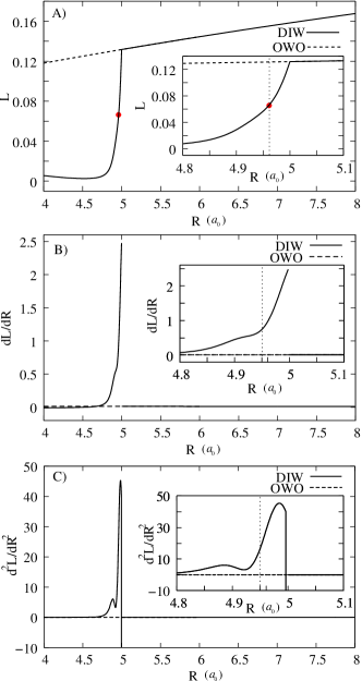
Figure 4: Panel A: Linear entropy ($L$) as a function of R for the DIW and OWO potentials. The dots indicates the value of $L_{DIW}$ at $R=R_{c}$. Panels B and C: first and second derivatives with respect to $R$ of the the linear entropy as a function of $R$. In all three panels, the inset represents the respective function around the migration point $R_{c}$, the latter being highlighted by the vertical dotted line.

The linear entropy of the DIW, $L_{DIW}$, and of the OWO system are compared in Fig. 4A. $L_{DIW}$ displays three regions. The first is characterized by a slow variation in entropy with a shallow minimum at $R=4.51\,a_{0}$. In the second region ($4.9\,a_{0}\lesssim R<5\,a$) the entropy increases very rapidly, and finally for $R>5a_{0}$ the entropy increases linearly with $R$. The first derivative of $L_{DIW}$ (Fig. 4B) presents a shoulder-like structure connecting the first and second regions; then, after the boost in the rate of change of the entropy, the derivative has a finite discontinuity at $R=5\,a_{0}$. The second derivative of $L_{DIW}$ presents two maxima at $R=4.89\,a_{0}$ and $R=4.99\,a_{0}$, and a minimum at $R=4.92\,a_{0}$. It has an infinite discontinuity at $R=5\,a_{0}$

The rate of change of the entropy shown in Fig. 4 is the result of the competing effects of the confinement strength and of the Coulomb repulsion. However, since it is the ratio between these two factors which governs the response of the system to a variation of the driving parameter, a maximum of $\left\langle U\right\rangle$ corresponds here to a minimum of the entanglement as these extrema occur when the electrons are most confined and hence in an almost factorized state.Abdullah et al. (2009) The decrease of $\left\langle U\right\rangle$ is a signature of the wavefunction spilling into the outer well and, consequently, of an increasing influence of Coulomb correlations in shaping the wavefunction with a corresponding increase of the entanglement. In the migration region (with $\left\langle U\right\rangle(R_{c})$ being approximately $7\%$ of its maximum value), the wavefunction density is substantially spread within the outer well, and small variations of $R$ produce large changes in the entanglement.

We note that in Ref. Marchisio et al., 2010, a system similar to DIW, with an inner well shrinking in width but never disappearing, was studied. In this a case no discontinuity in any derivative of the relevant quantities were found.

III.3 Comparison between the DIW and the OWO potentials

In Figs. 2A and 4A $E_{0}$ and $L$ are plotted for both the OWO and DIW potential. At $R=R_{c}$ the many-body ground-state is bounded to the outer well, and in particular $E_{0}^{DIW}(R_{c})\approx 0.99E_{0}^{OWO}(R_{c})$. In contrast, $L_{DIW}(R_{c})$, which is marked by a dot in Fig. 4, is approximately half of the corresponding entanglement value in the OWO case. We underline that here the inner well has a finite depth but the inner to outer well ratio is only $0.0039$, so, from a geometric point of view, the inner well should be negligible. However in the region $R_{c}\leq R<5$ the behavior of $\left\langle U\right\rangle$, with $\left\langle U\right\rangle_{DIW}>\left\langle U\right\rangle_{OWO}$, suggests that the electrons remain strongly pinned to the inner well region even though the width of the latter is basically negligible. As a consequence a very narrow inner well is able to modify the distribution of the electrons in such a way that their entanglement is highly and non-linearly reduced. This ‘pinning property’ of the entanglement might open possibilities of rapidly and efficiently modifying the entanglement in a nanostructure system.

IV Ground-state wavefunction and particle-density behavior

In Fig. 5 the high sensitivity of the system wavefunction to small changes of the driving parameter in the migration region is explicitly demonstrated. The figure in fact shows the wavefunction contour plots for $R=4.5\,a_{0}$ ($\sim$ maximum of $\left\langle U\right\rangle_{DIW}$, panel A), $R=R_{c}$ (‘migration’ point, panel B) and $R=5\,a_{0}$ (value at which the inner well disappears, panel C). The wavefunction becomes more and more confined until $R\approx 4.5\,a_{0}$, for which it displays a single maximum (panel A). A further reduction of the inner well width induces the wavefunction to leak into the outer well (compare scales on axis of panels A and B). Around $R\approx R_{c}$ the wavefunction starts to separate into two lobes, but remains largest close to the inner well (pinning effect). As $R$ increases beyond $R_{c}$, the shape of the wavefunction displays two well-defined lobes, reflecting the effect of the electron-electron repulsion combined with the diminished confinement strength (panel C). The wavefunction width and height though remain roughly constant, compare panels B and C. We note that the wavefunction shape appears to change “smoothly” as $R$ increases and, in particular, no detectable change in the geometry of the wavefunction seems to take place at $R=5\,a_{0}$, where the non-differentiable points of the entropy and energies are both located.

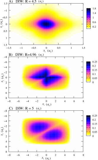
Figure 5: (color online) Contour plot of the wavefunction against the particles’ positions $x_{1}$ and $x_{2}$ for the DIW potential at $R=4.5\,a_{0}$ ($\sim$ maximum of $\left\langle U\right\rangle_{DIW}$ and minimum of $L$, panel A), $R=R_{c}=4.96\,a_{0}$ (panel B), and $R=5\,a_{0}$ (point at which $W^{iw}_{DIW}=0$, panel C).

As already mentioned, the particle density $n(x;R)$ should uniquely capture the system ground-state behavior, so we will now check if the density shape is more susceptible than the wavefunction to the shrinking and disappearance of the inner well. In Fig. 6 the density is plotted for various values of $R$. We see that, as $R$ increases, the height of the central (and only) peak diminishes. For $R\approx R_{c}$ the density develops two shoulders and at $R=5\,a_{0}$ the central peak disappears and is replaced by two peaks which are symmetric around the origin. This can more clearly be seen in the inset. At least for the system at hand, the pinning from the inner well has a more clear-cut effect on the shape of the density than on the shape of the wavefunction, as in particular it determines the presence or absence of a central peak for the particle density. At difference with the wavefunction, the change in the number of peaks of the particle density associated to the disappearance of the central maximum can then be associated with the discontinuity in the derivatives of energy and entanglement caused by the disappearance of the inner well.

Figure 6: Density $n(x;R)$ for the DIW potential plotted against the position $x$ for four different values of $R$ (as labeled). Inset: zoom of main panel for $R\approx 5$.

V Fidelity of the ground-state wavefunction

The fidelity between two states quantifies their similarity and as such has been extensively used in quantum information theory.Nielsen and Chuang (2000) More recently the fidelity has been introduced as a method for the characterization of QPTs:Zanardi and Paunković (2006); Zanardi et al. (2007); Campos Venuti et al. (2008) a signature of QPT is an abrupt change in the wavefunction,Sachdev (2000) and this suggests the evaluation of the fidelity between states across the critical point as a good choice for the identification of a QPT. Here we will use this method to better understand the system behavior in the migration region.

For our system the ground-state fidelity is given by

$$F(R_{1},R_{2})=|\left\langle\psi(x_{1},x_{2};R_{1})\left|\psi(x_{1},x_{2};R_{2})\right.\right\rangle|;$$ (16)

following Eq. (12) we then calculate it as $F(R_{1},R_{2})=\left|\sum_{j1,j2=1}^{M}a_{j_{1},j_{2},n}(R_{1})a_{j_{1},j_{2},n}(R_{2})\right|$. $F(R_{1},R_{2})$ can be interpreted in two complementary ways,Wootters (1981) and according to this we will consider two different sets of values for $R_{1}$ and $R_{2}$.

In quantum information theory, the fidelity can be seen as a generalization of a measure of similarity between two classical probability distributions.Nielsen and Chuang (2000) Let us take $R_{1}=R_{0}$, where $\psi(R_{0})$ is the reference state, then the fidelity is the overlap between this initial state and the wavefunction $\psi(R)$ calculated as $R_{2}=R$ varies in the parameter space. The fidelity $F(R_{0},R)$ clearly depends on the choice of the reference state. The fact that the minimum of the entanglement corresponds to a quasi-product state (see Fig. 4, panel A), which evolves towards a highly entangled state as $R$ increases, suggests as a natural choice $R_{0}=4.52\,a_{0}$, corresponding to the minimum of the linear entropy.

Alternatively, the fidelity can be seen as a geometrical object connected to the Fubini-Study distance between quantum states,Zanardi et al. (2007) where the square distance between infinitesimally close states can be approximated as $ds_{FS}^{2}\approx 2(1-F)$. In this case the fidelity is calculated between two wavefunctions depending on infinitesimally different parameters, $\psi(R)$ and $\psi(R+\delta R)$. At the critical point, where there is an abrupt change in $\psi$, this function has a minimum and possibly a discontinuity.

Figure 7: Panel A: fidelity $F(R_{0},R)$ vs $R$ for $R_{0}=4.52\,a_{0}$. Inset: first derivative of $F(R_{0},R)$ vs $R$. Panel B: fidelity $F(R,R+\delta R)$ vs $R$ with $\delta R=0.002$. Inset: as for the main panel, but zooming on the region of the fidelity minimum. The plots refer to the DIW and OWO potential (as labeled); the vertical dotted line corresponds to $R_{c}$.

In Fig. 7, the fidelities $F(R_{0},R)$ and $F(R,R+\delta R)$ are plotted as a function of $R$ (panel A and B, respectively). $F(R_{0},R)$ displays three distinct regimes, in accordance with the behavior of all the other quantities studied so far. In particular, we see that for $4.8\,a_{0}\lesssim R<5\,a_{0}$ we have a dramatic decrease of the fidelity: the wavefunction is rapidly changing from a quasi-product state towards a triplet-like entangled stateAbdullah et al. (2009) (compare Fig. 5, panels A and C). The derivative $dF(R_{0},R)/dR$ presents a minimum at $R\approx 4.92\,a_{0}$, near the migration point $R_{c}$. For $R>5\,a_{0}$ the fidelity is almost constant and drastically reduced, with $F(R_{0},R=5)\approx 0.19$: in this region the wavefunction is nearly orthogonal to the reference state. We note that $F(R_{0},R)$ is not differentiable at $R=5\,a_{0}$.

The behavior of $F(R,R+\delta R)$ (Fig. 7B) shows that the most significant changes in the wavefunction are confined to the migration region, around a marked minimum at $R=4.93$, again very close to $R_{c}$. $F(R,R+\delta R)$, which for real wavefunctions and $N$ particles can be approximated as

$$F(R,R+\delta R)\approx 1-\frac{\delta R^{2}}{2}\!\!\int\!\!\left(\frac{\partial\psi(x_{1}\ldots x_{N};R)}{\partial R}\right)^{2}\!\!\!\!dx_{1}\ldots dx_{N},$$ (17)

shows a discontinuity at $R=5\,a_{0}$, in accordance with the discontinuity found in the derivatives of all the quantities discussed so far.

VI Fidelity of the particle density

For a $1$-particle system with control parameter $R$ we have that the particle density is $n(x;R)=|\psi(x;R)|^{2}$ so, in this case, the fidelity may be written in terms of the density as $F(R_{1},R_{2})=\int\sqrt{n(x;R_{1})n(x;R_{2})}dx$.

We may generalize this to a ‘density fidelity’ by using the density arising from $N$-particle systems,

$$n(x,R)=N\int|\psi(x,x_{2}\ldots,x_{n};R)|^{2}dx_{2}\ldots dx_{n}.$$ (18)

and defining the ‘density fidelity’ as

$$F_{n}(R_{1},R_{2})=\frac{1}{N}\int\sqrt{n(x;R_{1})n(x;R_{2})}dx.$$ (19)

$F_{n}(R_{1},R_{2})$ has the properties expected from a fidelity, that is $0\leq F_{n}(R_{1},R_{2})\leq 1$ and it measures the overlap between particle densities as the driving parameter $R$ is varied. We will also demonstrate that $F_{n}(R_{1},R_{2})$ vanishes if and only if the corresponding wavefunction fidelity $F(R_{1},R_{2})$ vanishes.

We note that a density fidelity has been proposed for lattice systems and linked with QPTs in Ref. Shi-Jian, 2009. We initially calculate the density fidelity with respect to $R_{0}$. $F_{n}(R_{0},R)$ shows a non-differentiable point at $R=5\,a_{0}$ corresponding to the disappearance of the inner well (Fig. 8A); its derivative in respect to $R$ is plotted in the inset. We note the similarity between the behavior of $F_{n}(R_{0},R)$ and $F(R_{0},R)$ and between their derivatives, the main difference being that the residual fidelity for $R>\,5a_{0}$ is larger for the density than for the wavefunction.

Figure 8: Panel A: Density fidelity $F_{n}\left(R_{0},R\right)$, $R_{0}=4.52\,a_{0}$, for the DIW system, plotted against the parameter $R$. Inset: Derivative of $F_{n}\left(R_{0},R\right)$ with respect to $R$ plotted against $R$ ($R_{0}=4.52\,a_{0}$). Panel B: $F_{n}\left(R,R+\delta R\right)$ with $\delta R=0.002$, plotted against the parameter $R$ for the DIW system.

We show $F_{n}(R,R+\delta R)$, where $\delta R=0.002$, in Fig. 8 (panel B). As for the corresponding wavefunction fidelity, here the discontinuity at $R=5\,a_{0}$ appears directly in the ‘density fidelity’. Again the behavior of $F_{n}(R,R+\delta R)$ and $F(R,R+\delta R)$ are very similar (compare Fig. 8B with the inset of Fig. 7B), with the density preserving a slightly higher fidelity at its minimum, which occurs at $R=4.92\,a_{0}$

In the DIW system, viewing the density seems to more clearly and readily display the fast changes in the ground state properties corresponding to the discontinuity in the derivatives of $E_{0}$ and $L$ than viewing the wavefunction (see comments to Figs. 5 and 6). This may be due to the lesser formal complexity of the density, which is always a function of a single position vector – $x$ in the present case – as opposed to the complex many-body wavefunction, a function of $N$ position vectors whose parameter space is clearly more difficult to analyse and visualize. In addition the particle density fidelity is able to predict all the other notable features of the wavefunction fidelity, such as the minimum occurring around $R\approx R_{c}$. As noted, minima in the fidelity $F(R,R+\delta R)$ are associated to abrupt changes in the wavefunction and may signal the occurrence of a QPT, so, in accordance with Ref. Shi-Jian, 2009, our results suggests that the density fidelity may be used as an alternative to the wavefunction fidelity to understand brisk changes in the ground state and hence to study QPTs. This is in line with the Hohenberg-Kohn theorem which in its simplest form shows that for non-degenerate ground-states, the density uniquely determines the many-body wavefunction and so all the properties of the system.Hohenberg and Kohn (1964) We point out that the particle density is a much easier quantity to calculate (and to experimentally access) than the full many-body wavefunction. As such the use of the fidelity density might become of great help in understanding phenomena such as QPTs. Similarly its characteristics as highlighted above suggest that it could be a useful tool for local sensitivity analysis.

VI.1 One-to-one correspondence between vanishing of ground state particle density fidelity and wavefunction fidelity

We will now demonstrate the important property that, for systems with finite external potentials and ground-states with nodeless spatial wavefunctions, the density fidelity is zero if and only if the ground-state spatial wavefunction fidelity is zero.

The nodeless spatial ground-state wavefunction of a time-independent Hamiltonian may always be taken to be real and positive, so for any two such $N$-particle ground-state wavefunctions $\psi_{1}$ and $\psi_{2}$ we may define the real positive function

$$f_{1,2}(x)\equiv\int\psi_{1}\psi_{2}dx_{2}\dots dx_{N}.$$ (20)

For any fixed $x$ this defines an inner product, as positive definiteness is satisfied by $f_{1,1}(x)=n(x)/N>0$ for finite external potentials. The Cauchy-Schwarz inequality can then be written as

$$\int\psi_{1}\psi_{2}dx_{2}\ldots dx_{N}$$

$$\leq\left(\int\left|\psi_{1}\right|^{2}dx_{2}\dots dx_{N}\int\left|\psi_{2}\right|^{2}dx_{2}\dots dx_{N}\right)^{\frac{1}{2}}.$$ (21)

integrating both sides with respect to $x$ leads to

$$F\leq F_{n}$$ (22)

and so if $F_{n}$ tends to zero, so must $F$.

For a general wavefunction, a fidelity of zero does not imply a density fidelity of zero as for example two excited state wavefunctions may both be non-zero in some finite region of space but still be orthogonal. In addition, if we compare wavefunctions arising from different forms of inter-particle interactions, say attractive and repulsive, then, again, the density cannot always discriminate between orthogonal wavefunctions. This can be explicitly seen by considering the limiting case of infinite inter-particle attraction or repulsion. Let us consider two particles in one dimension: in the case of infinite attraction their wavefunction will satisfy $\psi_{A}(x_{1},x_{2})=0$ if $x_{1}\neq x_{2}$, while for infinite repulsion we have $\psi_{R}(x_{1},x_{2})=0$ if $x_{1}=x_{2}$, otherwise both $\psi>0$. Clearly we obtain $\int\psi_{A}\psi_{R}dx_{1}dx_{2}=0$. Let us now consider the single particle densities. In general it will be $n_{R}(x)=\int|\psi_{R}(x,x_{1})|^{2}dx_{1}>0$. To ensure normalization, $\psi_{A}(x_{1},x_{2})^{2}=\phi_{1}(x_{1})^{2}\delta(x_{1}-x_{2})$, with $\phi_{1}(x_{1})$ itself normalized, giving a corresponding single particle density $n_{A}(x)=|\phi_{1}(x)|^{2}>0$. It follows that the related density fidelity $\int\sqrt{n_{R}(x)n_{A}(x)}dx$ is different from zero.

However, if we assume the requirements needed for standard DFT, i.e. ground state and same inter particle interaction, then we can argue that the density fidelity can detect orthogonal, nodeless ground-state wavefunctions. The lack of nodes in the ground states means that we can choose a phase so that both our wavefunctions are never negative. Here a fidelity of zero corresponds to the hypothetical situation when the wavefunctions do not overlap at all. When the inter particle interaction is fixed this lack of overlap arises because the wavefunctions are spatially distinct, and so the densities will not overlap. Hence for ground-states with nodeless spatial wavefunctions, the density fidelity is zero if and only if the spatial wavefunction fidelity is zero.

VII QPT-like transition (symmetric systems)

As pointed out previously, a minimum in $F(R,R+\delta R)$ may highlight a QPT and certainly witnesses a rapid change in the wavefunction. In our case the, minimum in $F(R,R+\delta R)$ observed in Fig. 7 corresponds to the transition between two separate sets of ground states; the first set bounded by the inner and the second set bounded by the outer well. Fig. 7A shows that this transition is between states that are almost orthogonal. As the width of the inner well is reduced, the energy gap between these set of states reduces: this transition has some of the characteristics of a second-order QPT.

This is apparent when looking at the ground state energy derivatives: $d^{2}E_{0}/dR^{2}$ presents in this region a marked minimum, which in turn corresponds to an inflection point in the energy first derivative. If this were a full-fledged QPT, this inflection point would have a vertical tangent, and hence the minimum in $d^{2}E_{0}/dR^{2}$ would become a divergency.

As discussed in Refs Wu et al., 2006 and Wu et al., 2004, a second-order QPT should be signaled by a corresponding structure in the first derivative of the entanglement. The first derivative of the entanglement entropy presents indeed a structure (a shoulder) whose width can be defined by the first maximum-minimum structure in $d^{2}L/dR^{2}$, i.e $4.89\,a_{0}\leq R\leq 4.92\,a_{0}$ (see Fig.4, panels B and C): this shoulder indeed frames the region of the minimum of $d^{2}E_{0}/dR^{2}$. The bulk of the wavefunction change should occur in the region of the minimum of $F(R,R+\delta R)$: in Fig. 9 we then present the wavefunction at $R=4.91\,a_{0}$ (panel A) and $R=R_{c}=4.96\,a_{0}$ (panel B). The plots confirm a quite substantial change in the wavefunction, which smears over the upper well as $R$ increases, changing from a single, pointed peak towards a two-lobe geometry.

As for the case of a finite-size system which would undergo a QPT in the thermodynamic limit,Osterloh et al. (2002) the transition we observe in the wavefunction occurs over a (small) parameter region and slightly away from the expected ‘critical’ value of the driving parameter, i.e., for $R\lesssim R_{c}$.

Figure 9: Ground-state wavefunction plotted against the particles’ positions $x_{1}$ and $x_{2}$ for the DIW potential at $R=4.91\,a_{0}$ , panel A, and $R=R_{c}=4.96\,a_{0}$, panel B.

VIII Origin of the discontinuities observed at $R=w$

It was demonstrated in Ref. Wu et al., 2006, 2004 that a discontinuity in the first (second) derivative of the ground-state energy with respect to the driving parameter – a signal of a QPT – may correspond to a discontinuity in the (derivative of the) ground-state entanglement.

What we observe in the present case at $R=w$ is instead a discontinuity in the same order derivatives of the ground-state energy and entanglement. Moreover, all the other quantities under study, such as $\left\langle U\right\rangle$ or $S_{n}$, are non-differentiable at the same point. A similar situation was speculated for the limit $p\to\infty$ in Ref. Abdullah et al., 2009. Here we would like to clarify the origin of the discontinuities we observe.

First of all we can extract from the fidelities important information on the ground state wavefunction behavior at $R=w$: the continuity of $F(R_{0},R)$ shows that the ground-state wavefunction is continuous, on average, at $R=w$ (see Fig. 7A). However the discontinuity of $\partial F(R_{0},R)/\partial R|_{R=w}$ indicates a discontinuous derivative for the wave function at the same point (inset of Fig. 7A). The discontinuity of $\partial\psi(\bm{x};R)/\partial R$ at $R=w$ is confirmed by the discontinuity of $F(R,R+\delta R)$ at the same point, see Eq. (17).

To understand the above picture we consider the Hamiltonian for a general potential

$$H(R)=H_{0}+\sum_{j}V(x_{j},R),$$ (23)

where $H_{0}={T}+{{U}}$ is independent from the driving parameter $R$, $T$ is the kinetic energy, and ${U}$ is the electron-electron interaction. From the Hellmann-Feynman theorem we have

$$\frac{dE(R)}{dR}=\sum_{j}\left\langle\psi(\bm{x};R)\left|\frac{\partial V(x_{j};R)}{\partial R},\right|\psi(\bm{x};R)\right\rangle,$$ (24)

where $\bm{x}=(x_{1},\dots x_{N})$ represents the coordinates of the $N$ particles. Consequently, if $\partial V(x_{j};R)/\partial R$ is discontinuous with respect to the parameter $R$, then this discontinuity could propagate to $d{E}/d{R}$.

We note that in the case of a first order QPT, the discontinuity in $d{E}/d{R}$ should arise from the wavefunction, and not from the potential. In the present case, while the fidelity indicates a continuous wavefunctions, not only $d{E}/d{R}$, but also all the other quantities used as indicators for a QPT, present a point of non-analyticity at $R=w=5\,a_{0}$. It is hence necessary to understand how a discontinuity in the potential would affect the other quantities of interest, and in particular if, in contrast with the situation in Refs. Wu et al., 2004, Wu et al., 2006, it would produce discontinuities in the first derivative of both energy and entanglement entropies.

By considering the time-independent Schrödinger equation associated to Eq. (23) we can write

$$-\frac{T\psi(\bm{x};R)}{\psi(\bm{x};R)}-\frac{{U}\psi(\bm{x};R)}{\psi(\bm{x};R)}+E(R)=\sum^{2}_{j=1}V(x_{j};R).$$ (25)

Eq. (25) is well-defined for a nodeless ground state wavefunction and can be seen as a family of equations labeled by the continuous parameter $R$. Eq. (25) shows that if the potential is discontinuous only at a set of points of measure zero then, at most, it may only directly cause $\psi$ and/or $T\psi$ to be discontinuous on that same set of points. Hence, for finite discontinuities, these discontinuities will not propagate to any integrated quantities such as expectation values. We then continue by assuming that $\psi$ and ${T}\psi$ are, at worst, discontinuous over a set of points of measure zero. We differentiate Eq. (25) with respect to $R$, and use Eq. (24) to obtain

$$-\frac{1}{\psi(\bm{x};R)}T\frac{\partial{\psi(\bm{x};R)}}{\partial{R}}+\frac{\left[T\psi(\bm{x};R)\right]}{\psi^{2}(\bm{x};R)}\frac{\partial{\psi(\bm{x};R)}}{\partial{R}}$$

$$=\sum_{j}\left[\frac{\partial V(x_{j};R)}{\partial R}-\left\langle\psi(\bm{x};R)\left|\frac{\partial V(x_{j};R)}{\partial R}\right|\psi(\bm{x};R)\right\rangle\right].$$ (26)

Finite discontinuities in the potential may mean that its derivative with respect to $R$ will comprise delta functions, and hence that, unless accidental cancellations occur, these discontinuities will propagate to $\left\langle\partial{V(x_{j};R)}/\partial{R}\right\rangle$. Let us assume that they are such that $\left\langle\partial{V(x_{j};R)}/\partial{R}\right\rangle$ is discontinuous at $R=\tilde{R}$. Then, on the right-hand side of Eq. (26) we have two discontinuous functions with respect to $R$, but as the second term does not depend on $\bm{x}$, the right-hand side is actually discontinuous at $(\bm{x};\tilde{R})$ for all or almost all values of $\bm{x}$ since no accidental cancellations can hold for all $\bm{x}$. This means that the left hand side of Eq. (26) will present the same discontinuities. As $\psi(\bm{x};R)$ and $T\psi$ are at least continuous almost everywhere with respect to $\bm{x}$ at $(\bm{x};\tilde{R})$, this implies that $\partial{\psi(\bm{x};R)}/{\partial{R}}$ has indeed to be discontinuous at $(\bm{x};\tilde{R})$ for all or almost all $\bm{x}$ and hence the first derivative in respect to $R$ of any functional of $\psi$ will be in general discontinuous at $R=\tilde{R}$. This is exactly what we observe.

In Appendix A1 we illustrate these points by explicitly analyzing the effect of the finite discontinuity at the point $(x=0;R=w)$ in $V_{DIW}$.

In the next section we will instead consider a counter-example for which, due to an accidental cancellation, $\left\langle\partial{V(x_{j};R)}/\partial{R}\right\rangle$ – and hence all first derivatives in respect to $R$ – remains continuous even in the presence of discontinuities in $V(x_{j};R)$ similar to the ones of the DIW potential.

IX Core-shell to double well potential

In Ref. Abdullah et al., 2009 it was speculated that, in the rectangular-like potential limit, the observed sharp transitions in energies and entanglement would display non-analyticities as the potential changes from a core-shell structure to a double well potential. The behavior of the entanglement and its derivatives in this limit is shown in Fig. 10.

Figure 10: Upper panel: Entanglement entropy $L$ plotted against $R$ for the potential of Eq. (11) and $w=5a_{0}$. Inset: same as main panel but plotted in respect to $R_{DW}$ for an easier comparison with Ref. Abdullah et al., 2009. Middle panel and lower panel: $dL/dR$ and $d^{2}L/dR^{2}$, respectively, vs $R$ for the potential of Eq. (11) and for $w=5\,a_{0}$. The insets present the transition region and the vertical dotted line the migration point $R_{c}=4.98\,a_{0}$ for the potential Eq. (11).

Figure 11: Panel A, B and C: $d^{2}E_{0}/dR^{2}$, $F(R_{0},R)$ and $F(R,R+\delta R)$ for the DW potential with respect to $R$. The insets in panel A and C present the details of the transition region; the inset in B depicts the first derivative of $F(R_{0},R)$ with respect to $R$ and with $R_{0}=4.76a_{0}$.

For the DW potential Eq. (11), the plot of $F(R_{0},R)$ (Fig. 11B, with $R_{0}=4.76a_{0}$ the minimum of $L$ for this system) confirms that the reference state, almost factorized and bounded to the inner well, is practically orthogonal to the triplet-like ground state reached after the transition to the double well potential.Abdullah et al. (2009) However a QPT-like transition occurs only when the ground state bounded to the inner well migrates to the outer well, see the shoulder in $dL/dR$ and the minimum of $d^{2}E_{0}/dR^{2}$ in Figs. 10B and 11A, respectively. The subsequent transition to a double-well potential merely further isolates the two lobes of the wavefunction from each other. The sharp increase in entanglement which corresponds to this further change, does not then signal any further QPT-like point, as confirmed by the absence of additional structures in $d^{2}E_{0}/dR^{2}$ and $F(R,R+\delta R)$ (see Fig. 11A and Fig. 11C).

Interestingly, in contrast with the DIW case, the discontinuity at $R=w$ of $\left\langle\partial{V(x_{j};R)}/\partial{R}\right\rangle$ is accidentally removed in this system. As a result the derivatives with respect to $R$ of the various quantities of interest, as well as $F(R,R+\delta R)$, do not present discontinuities (see Figs. 10 and 11). Details are given in Appendix A2.

X Asymmetric potential

We will now consider the possibility for the position of the inner well, with respect to the symmetry axis of the outer well, to be shifted toward left (see Fig. 12, upper panels) and we will refer to these asymmetric potentials as Asymmetric Disappearing inner Well (ADW) potentials. In Fig 12D, the inner well position is left-shifted by a quantity $w_{a}=2\,a_{0}$, where $w_{a}$ is the distance between the symmetry axes of the inner and outer well. In panels 12C and 12B, $w_{a}=1.5\,a_{0}$ and $w_{a}=1\,a_{0}$, respectively, while the system described in panel 12A, which represents the symmetric case $w_{a}=0\,a_{0}$, is taken as benchmark. The width of the inner well follows Eq. (4) with $w=5\,a_{0}$, shrinking from $W^{iw}=1\,a_{0}$ for $R=4\,a_{0}$ to $W^{iw}=0\,a_{0}$ for $R=5\,a_{0}$. The width of the outer well is assumed constant, $W^{ow}=w$. The depth of the wells is $V^{ow}_{0}=-15$ Hartree and s $V^{iw}_{0}=-10$ Hartree for the outer and inner well discontinuity (barrier) rispective. Henceforth, the letters A, B, C, D are used to indicate the four systems whose potential is depicted in the respective panels of Fig 12.

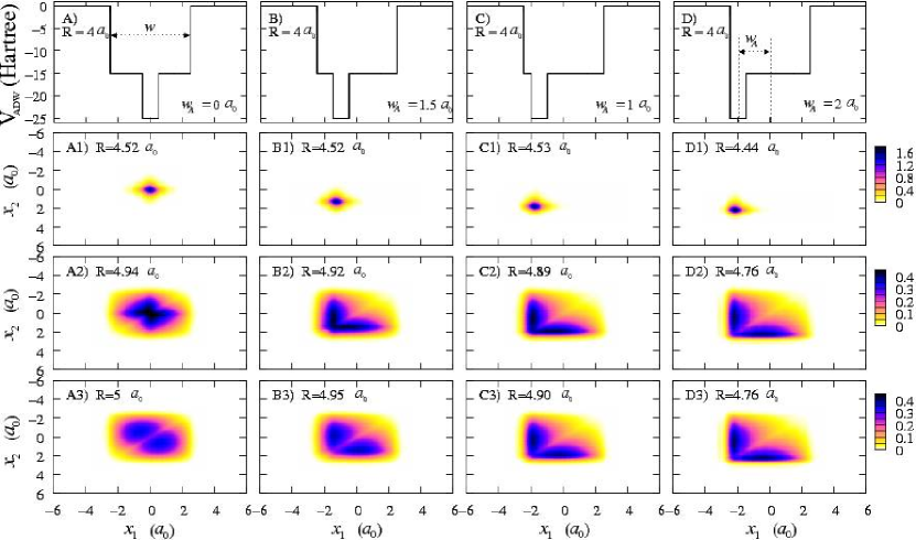
Figure 12: (Color online) Panels B to D: Asymmetric Disappearing inner Well (ADW) potential $w_{a}=1\,a_{0}$ Vs the coordinate $x\equiv x_{1}$. Panel B and C, same as above but for $w_{a}=1.5\,a_{0}$ and $w_{a}=2\,a_{0}$. Panel A: symmetric case ($w_{a}=0\,a_{0}$). Panels A1 to D1: Contour plots of the wavefunction against the particles’ positions ($x_{1}$, $x_{2}$) at the minimum of $L(R)$. Panels A2 to D2: same as above but in correspondence of the ‘migration’ point. Panels A3 to D3: same as above but in correspondence of the maximum of the entropy.

The entanglement (linear entropy) and its derivatives, $dL/dR$ and $d^{2}L/dR^{2}$, are plotted in the three panels of Fig. 13, respectively. For $R\approx 4\,a_{0}$, the many-body wavefunction is well-confined inside the inner well. Thus the entanglement of systems A to D shows there approximately the same behaviour, independently of the position of the inner well with respect to the symmetry axis of the outer well. The second row of panels in Fig 12, namely A1,B1,C1 and D1, shows the contour plots of the two-body wavefunction with respect to the particles’ coordinates $x_{1}$ and $x_{2}$ in correspondence of the minimum of the linear entropy. With the exception of the case D ( Fig. 12D1 ), the contour plots are very similar where the wavefunction is significantly different from zero. This, in turn, is reflected in a similar position of the minimum of the linear entropy. In fact, using the subscripts A, B, C and D to indicate the four potentials, we have that the minima of $L(R)$ are at $R_{A}=4.52\,a_{0}$, $R_{B}=4.52\,a_{0}$, $R_{C}=4.53\,a_{0}$, and $R_{D}=4.44\,a_{0}$.

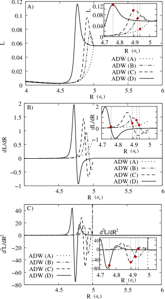
Figure 13: Panel A, B and C: $L(R)$, $dL/dR$ and $d^{2}L/dR^{2}$ plotted as a function of the driving parameter $R$ for the four potentials depicted in Fig. 12. The region of major variations of these quantities are detailed in the inset inside the respective panels. The dotted vertical lines highlight the migration point for each potential.

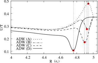
Figure 14: Ratio $\langle U\rangle/\langle T\rangle$ (Coulomb energy over kinetic energy) for the four potential represented in Fig. 12 with respect to $R$. The dotted vertical lines highlight the migration point for each case A, B, C and D.

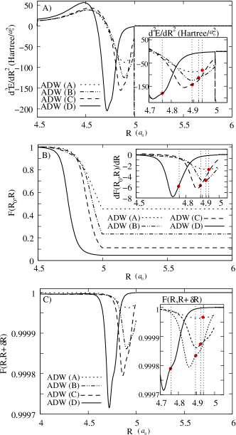
Figure 15: Panel A, B and C: $d^{2}E/dR^{2}$, $F(R_{0},R)$ and $F(R,R+\delta R)$ plotted as a function of the driving parameter $R$ for the four potentials depicted in Fig. 12. $R_{0}$ is the value of the parameter at which $L(R)$ reaches its minimum for each potential in Fig. 12, where $\delta R=0.002\,a_{0}$ for all four cases. The inset represent the region around the migration point for the panels $A$ and $C$, while in panel $B$ the inset depicts the derivative of $F(R_{0},R)$ with respect to $R$. The dotted vertical lines highlight the migration point for each potential.

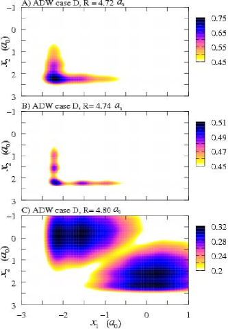
Figure 16: Panel A, B, C: Asymmetric Disappearing inner Well (ADW) case D. Contour plots of the wavefunction against the particles’ positions ($x_{1}$, $x_{2}$) at $R=4.72\,a_{0}$ (minimum of $d^{2}E/dR^{2}$ and $F(R,R+\delta R)$) $R=4.74\,a_{0}$ and $R=4.80\,a_{0}$ respectively

As $R$ increases, the ground-state approaches the migration point. Consequently, the particles become progressively bounded by very different confinement potentials: symmetric for A, and increasingly asymmetric from B to D. As the ground state wavefunction ‘spreads’ in the upper well, the larger is $w_{a}$, the more the wavefunction is distorted by a combination of the pinning effect due to the finite size of the inner well and the presence of the left hand side potential barrier of the outer well. The third row of panels in Fig 12 highlights the increasingly marked asymmetry in correspondence of the migration points, located at $R_{D}=4.76\,a_{0}$, $R_{C}=4.89\,a_{0}$, $R_{B}=4.92\,a_{0}$ and $R_{A}=4.94\,a_{0}$ (panels from A2 to D2).

The most interesting feature is, however, the marked maximum of the entanglement entropy for the three asymmetric potentials. In particular, the maximum of $L_{D}(R)$ is twice as large as the maximum value reached in the symmetric case. For the symmetric case, the maximum entanglement is reached at $R=5\,a_{0}$. The other maxima are located at $R_{D}=4.76\,a_{0}$, $R_{C}=4.90\,a_{0}$ and $R_{B}=4.95\,a_{0}$, hence the maximum of the entropy is reached at a value of $R$ which become closer and closer to the migration point as the asymmetry increases. For case D, the two values coincide. These and the appearance of the entanglement maxima may be understood by looking at Fig. 12A3 to Fig. 12D3, which display the contour plot of the wavefunction at the entanglement maxima: (i) the pinning effect localizes most of the wavefunction at the location of the inner well, while (ii) the reduced distance of outer well walls from the inner well in the asymmetric potentials further reduces the possibility for the wavefunction to significantly expand in the outer well. Due to (i) and (ii), as the asymmetry increases, the wavefunction becomes more strongly separated into two lobes and more strongly localized in two narrow peaks. These two characteristics imply that more information could be learned about the second particle position once the first is measured and hence means a larger entanglement with respect to the symmetric case. In particular, for case D, both (i) and (ii) are maximized at the migration point, which then corresponds to the maximum of the entanglement.

Using the same argument as in Sec. VIII, it is easy to show that the expectation value of the first derivative with respect to $R$ of the potential $ADW$, is discontinuous at $R=5\,a_{0}$. It follows that for this value of $R$, the function $L(R)$ is non-differentiable for all four cases, see Fig. 13B. Finally, we note that, for each asymmetric potential, the minimum of the second derivative of the entropy $d^{2}L/dR^{2}$ occurs approximately in correspondence of the migration point; while the extreme point of the ratio $\langle U\rangle/\langle T\rangle$ signals the migration point for both symmetric and asymmetric geometries of the confinement, see Fig. 14.

XI QPT-like transition (asymmetric systems)

Similarly to the symmetric case (see Sec. VII), also for asymmetric potentials the minimum of $d^{2}E/dR^{2}$ and of the fidelity $F(R,R+\delta R)$ is reached at the same value of the driving parameter: $R_{D}=4.72\,a_{0}$, $R_{C}=4.86\,a_{0}$, $R_{B}=4.89\,a_{0}$ and $R_{A}=4.91\,a_{0}$, see Fig. 15A and Fig. 15C. In addition, the minimum of $dF(R_{0},R)/dR$ also occurs at very similar values of $R$, namely $R_{D}=4.72\,a_{0}$, $R_{C}=4.87\,a_{0}$, $R_{B}=4.90\,a_{0}$ and $R_{A}=4.91\,a_{0}$. Notably the minima of $d^{2}E/dR^{2}$ and $F(R,R+\delta R)$ become the more pronounced the more asymmetric the system is.

The shoulder structure of $dL/dR$ observed in symmetric systems in correspondence to the migration point (and discussed in Sec. VII) develops now into a maximum-minimum structure (middle panel in Fig. 13). Here the maximum corresponds to the minimum of $d^{2}E/dR^{2}$ fairly precisely for systems B (maximum of $dL/dR$ at $R=4.90$, minimum of $d^{2}E/dR^{2}$ at $R=4.89$) and precisely for systems C and D. This coincidence of $d^{2}E/dR^{2}$ and $dL/dR$ extrema has been shown to signal QPTs in some systemsGu et al. (2003); Chen et al. (2006). We then expect the system at hand to display related characteristics, and in particular a rapid evolution between two (almost) orthogonal states. This is confirmed by Fig. 15B showing that when the driving parameter is swept across the minimum structure of $d^{2}E/dR^{2}$ ($4.5\lesssim R\lesssim 5$) the system rapidly evolves between two almost orthogonal states.

The minimum of $d^{2}E/dR^{2}$ and of $F(R,R+\delta R)$ becomes the more pronounced the more asymmetric the system is, indicating a more marked QPT-like behavior. We expect then a qualitative change of the wavefunction to occur on an even smaller parameter range, i.e. when sweeping the driving parameter just across the minimum itself. This is indeed the case: by looking at the wave-function countour plots for system D, we see that by sweeping the driving parameter in the range $4.71\lesssim R\lesssim 4.74$ the wavefunction evolves from having a single maximum positioned at the inner well, to having additional, marked, lateral maxima. These display the increasing importance of Coulomb correlations over confinement (compare Fig. 16 panels A and B).

Interestingly in the asymmetric systems the ‘migration’ point marks a secondary structure (a shoulder) on the right of the minimum of $F(R,R+\delta R)$ and $d^{2}E/dR^{2}$. In this region the wavefunction maximum located above the inner well disappears, and, due to Coulomb correlations, a valley develops between the wavefunction lobes (Fig. 16C).

The very narrow parameter region between the minimum of $F(R,R+\delta R)$ and $d^{2}E/dR^{2}$ and the ‘migration’ point represents the crossover from confinement to Coulomb correlations as the leading term in shaping the wave-function characteristics. In this region the entanglement is extremely sensitive to variations of the external parameter, going from its almost minimum to its maximum value (seeFig. 13). This very strong sensitivity could be exploited to envisage entanglement ’switches’.

XII Conclusions

We studied a set of systems of two electrons confined by a potential which evolves from a core-shell to a single well potential. For symmetric confining potentials (DIW system) as the driving parameter $R$ increases, the inner well width is reduced while the width of the outer well increases. The system ground state is initially bounded to the inner well with a wavefunction in a quasi-product state (entanglement minimum and Coulomb energy maximum). In the region around the point where the two electrons’ ground-state migrates into the outer well, the energy and the entanglement entropies are continuous and differentiable. However, here various QPT markers display a behavior similar to the one of a second-order QPT: in particular the second derivative of the ground state energy, as well as the fidelity $F(R,R+\delta R)$, displays a minimum, and the first derivative of the ground state entanglement presents a structure around this minimum. we then associate this parameter region to a ‘QPT-like’ transition. The wavefunction indeed undergoes here a drastic change, quickly evolving from a quasi-product towards a triplet-like state. We showed that a similar QPT-like transition characterizes also the evolution from a core-shell to a double-well potential described in Ref. Abdullah et al., 2009.

We compared the results for the DIW system with a benchmark system where only the outer well is present, and noticed that a very narrow inner well has a strong pinning effect on the entanglement (and fidelity) of the system. In particular for this symmetric system, the entanglement may be reduced by half by the presence of an inner well, even when the ground state is already bounded to the outer well.

We also consider systems (ADW) with the position of the core well being asymmetric with respect to the shell. We show that, in the ’migration’ region, their sensitivity to small variation of the driving parameter is even greater than for the symmetric case, with the entanglement displaying a sharp maximum at the ‘migration’ point and a value as high at twice the maximum value of a system without the inner well and about four times the value of a corresponding DIW system. This property might be exploited to create entanglement switches by moving the position of the inner well with respect to the outer well confining potential.

The maximum in the entanglement of ADW systems derives from a combination of the ’pinning effect’ by the inner core and of the asymmetric confinement (in respect to the pinning center) provided by the outer shell. This interplay results in the high probability of the second particle to be found in a more sharply defined small region of space, once the position of the first is measured, hence the increase in entanglement. In this region the analysis of QPT markers, and in particular the coincidence of the minimum of the energy second order derivative with the maximum of the entanglement entropy first order derivative, confirms a QPT-like behavior for the system wavefunction. This transition occurs in the region where, as the wavefunction expands from the inner to the outer well, Coulomb correlations starts to substantially modify its shape, and is due to the interplay between confinement by the core well, Coulomb interactions, and confinement by the outer well.

We demonstrated that a potential which is characterized by a driving parameter $R$ and has a finite discontinuity, even just at a single point $(\tilde{x},\tilde{R})$, may induce a discontinuity in the derivative of the ground-state wavefunction at $\tilde{R}$ for any (or almost any) value of $x$. This in turn induces a non differentiability at $\tilde{R}$, with respect to $R$, of any functional of the ground state and in particular – and in contrast with QPT signatures – of the same order derivatives of energy and entanglement. This is the case for the DIW potential described in this work: here the non-analytic behavior of ground state energy and entanglement, which is reminiscent of the one encountered in QPT, derives instead in a non-trivial way from the finite discontinuity at a single point of the confining potential. To underline the peculiarity of this connection we also presented a counter-example in which similar discontinuities in the potential do not transfer to other quantities. This is the case of the rectangular-like limit of the potential considered in Ref. Abdullah et al., 2009, where exact cancellations occur, and hence the ground state wavefunction and all related quantities, such as the entanglement and energy, remain differentiable at any $R$.

We presented a detailed analysis of the particle density fidelity, and showed that, for the ground state, this quantity provides similar information to the wavefunction fidelity, but may be calculated directly from the more accessible particle density. In particular we demonstrate that, for ground-states with nodeless spatial wavefunctions, the particle density fidelity is zero if and only if the wave function fidelity is zero.

Our results suggest that the entanglement of two particles confined in a controllable core-shell structure would display QPT-like characteristics as the ground states ‘migrates’ from the inner well to the outer shell, including a well defined minimum of both the wavefunction and particle density fidelities. In the corresponding narrow driving parameter range our calculations demonstrate a high sensitivity of the entanglement to variations of the core well size and/or position.

Finally our results show that the particle density fidelity may complement or perhaps even replace the traditional wavefunction fidelity as a diagnostic tool of the ground state of those systems for which the particle density may be experimentally accessed.

Appendix A Effect of the finite discontinuity of the confining potential

A.1 Core-shell to single well potential (DIW potential)

We note from Eq. (6) and Eq. (7) that $V_{DIW}(x;R)$ undergoes linear transformations (contraction of the inner well, dilatation of the upper well) which are continuous everywhere in $R$ with the exception of the point $(x=0;R=w)$. Treating the potentials $V_{DIW}(x;R)$ as a family of square integrable functions (this condition is verified for $R<\infty$), the usual distance can be defined and in particular we have that $D\big{(}V_{DIW}(x;w-\delta R),V_{DIW}(x;w)\big{)}=\sqrt{\int\left|V_{DIW}(x,w-\delta R)-V_{DIW}(x,w)\right|^{2}dx}$ goes to zero continuously as $\delta R\rightarrow 0$. This means that the disappearance of the inner well at $R=w$ marks the transition between two potentials which differ over a set of measure zero.

We now consider the expectation value of the derivative of our potential, $\langle{\partial V_{DIW}(x;R)}/{\partial R}\rangle$, which is directly related to the derivative of the ground-state energy, see Eq. (24).

Of the two components of $V_{DIW}$, see Eq. (8), only the derivative of $V^{iw}$ will contribute to a possible discontinuity at $(x=0;R=w)$, as the outer well is simply widening as $R$ increases. Its derivative is given by

$$\frac{\partial V^{iw}(x;R)}{\partial R}=$$

$$-\frac{V_{0}}{2}\left\{\delta\left(x+\frac{w-R}{2}\right)\theta\left(-x+\frac{w-R}{2}\right)\right.$$

$$+\left.\theta\left(x+\frac{w-R}{2}\right)\delta\left(-x+\frac{w-R}{2}\right)\right\}.$$ (27)

We can calculate $\langle{\partial V^{iw}(x;R)}/{\partial R}\rangle$ with the help of the property

$$\int_{-\infty}^{+\infty}n(x;R)\theta(\pm x+x_{0})\delta(\mp x+x_{0})dx=c_{x_{0}}n(\pm x_{0};R)$$ (28)

where $c_{x_{0}}=1$ for $x_{0}>0$, $c_{x_{0}}=0$ for $x_{0}\leq 0$. By using the symmetry $n(x;R)=n(-x;R)$ and considering $R<w$, we find

$$\left.\langle\frac{\partial V^{iw}(x;R)}{\partial R}\rangle\right|_{R<w}=-\frac{V_{0}}{2}n(W^{iw}/2;R).$$ (29)

On the other hand, for $R>w$, we obtain

$$\left.\langle\frac{\partial V^{iw}(x_{j};R)}{\partial R}\rangle\right|_{R>w}=0.$$ (30)

For $R\to w^{\pm}$, the above equations give

$$\left.\langle\frac{\partial V^{iw}(x;R)}{\partial R}\rangle\right|_{R\to w^{+}}-\left.\langle\frac{\partial V^{iw}(x;R)}{\partial R}\rangle\right|_{R\to w^{-}}=\frac{V_{0}}{2}n(0;w).$$ (31)

Here $n(0;w)$ is different from zero, and hence the expectation value of the derivative of the potential with respect to $R$ is discontinuous at $R=w$.

As a consequence, the derivative of the wavefunction with respect to $R$ is discontinuous at $(\bm{x};R=w)$ for all or almost all $\bm{x}$, and this explains the discontinuities observed in $F(R,R+\delta R)$ and $F_{n}(R,R+\delta R)$ and in the derivatives in respect to $R$ of entanglement, energies, $F(R_{0},R)$, and $F_{n}(R_{0},R)$.

A.2 Core-shell to double well potential (DW potential)

Similarly to the DIW potential, the potential in Eq. (11) displays a finite discontinuity in respect to $R$ at $(x=0;R=w)$.

For $R<w$, Eq. (11) is similar to the DIW potential except that in Eq. (11) the outer well decreases as the inner well does. For $R\geq w$, Eq. (11) describes two separated wells which move further apart and decrease in width as $R$ increases.

By repeating calculations similar to the ones done for $V_{DIW}$ we obtain

$$\left.\langle\frac{\partial V_{DW}(x_{j};R)}{\partial R}\rangle\right|_{R\to w^{\pm}}=-\frac{V_{0}}{2}\big{[}n\big{(}0;w)+n\big{(}w;w)],$$ (32)

which shows that no discontinuity appears in the limit $R\to w^{\pm}$ in the hypothesis that the wavefunction, and hence $n(x,R)$ is a continuous function of $R$: in this case, even if $\partial V_{DW}/\partial R$ does contain delta function-type discontinuities, there is no discontinuity in $\langle\partial V_{DW}/\partial R\rangle$ and hence the derivative of the wavefunction is continuous as well as the derivatives of the other functions discussed in this paper. This picture is confirmed by Fig. 10 where calculations performed directly with the square-well potential in Eq. (11) show a steep gradient of the entanglement at $R=w=5\,a_{0}$, but not a discontinuity in its derivative.

We remark that this cancellation of the discontinuity is accidental and is due to the fact that the depth of the inner well is the same as the height of the barrier between the double-well structure. The discontinuity reappears if this symmetry is lifted.

References

- Abdullah et al. (2009) S. Abdullah, J. P. Coe, and I. D’Amico, Phys. Rev. B 80, 235302 (2009).
- Nielsen and Chuang (2000) M. A. Nielsen and I. L. Chuang, Quantum Computation and Quantum Information (Cambridge University Press, 2000), ISBN 521635039.
- Larsson and Johannesson (2006) D. Larsson and H. Johannesson, Phys. Rev. A 73, 042320 (2006).
- Larsson and Johannesson (2005) D. Larsson and H. Johannesson, Phys. Rev. Lett. 95, 196406 (2005).
- Chen et al. (2006) Y. Chen, P. Zanardi, Z. D. Wang, and F. C. Zhang, New Journal of Physics 8, 97 (2006).
- Anandan (1991) J. Anandan, Journal Foundations of Physics 21, 1265 (1991).
- Zanardi and Paunković (2006) P. Zanardi and N. Paunkovi, Phys. Rev. E 74, 031123 (2006).
- Zanardi et al. (2007) P. Zanardi, P. Giorda, and M. Cozzini, Phys. Rev. Lett. 99, 100603 (2007).
- You et al. (2007) W.-L. You, Y.-W. Li, and S.-J. Gu, Phys. Rev. E 76, 022101 (2007).
- Amin and Choi (2009) M. H. S. Amin and V. Choi, Phys. Rev. A 80, 062326 (2009).
- Rezakhani et al. (2010) A. T. Rezakhani, D. F. Abasto, D. A. Lidar, and P. Zanardi, arxiv (2010).
- Quan et al. (2006) H. T. Quan, Z. Song, X. F. Liu, P. Zanardi, and C. P. Sun, Phys. Rev. Lett. 96, 140604 (2006).
- Roch et al. (2009) N. Roch, S. Florens, V. Bouchiat, W. Wernsdorfer, and F. Balestro, Nature 453, 633 (2009).
- Oh (2009) S. Oh, Physics Letters A 373, 644 (2009).
- Loss and DiVincenzo (1998) D. Loss and D. P. DiVincenzo, Phys. Rev. A 57, 120 (1998).
- Burkard et al. (1999) G. Burkard, D. Loss, and D. P. DiVincenzo, Phys. Rev. B 59, 2070 (1999).
- Reina et al. (2000) J. H. Reina, L. Quiroga, and N. F. Johnson, Phys. Rev. A 62, 012305 (2000).
- Biolatti et al. (2002) E. Biolatti, I. D’Amico, P. Zanardi, and F. Rossi, Phys. Rev. B 65, 075306 (2002).
- Li et al. (2003) X. Li, Y. Wu, D. Steel, D. Gammon, T. H. Stievater, D. S. Katzer, D. Park, C. Piermarocchi, and L. J. Sham, Science 301, 809 (2003).
- Pazy et al. (2003) E. Pazy, E. Biolatti, T. Calarco, I. D’Amico, P. Zanardi, F. Rossi, and P. Zoller, Europhys. Lett. 62 (2003).
- Feng et al. (2004) M. Feng, I. D’Amico, P. Zanardi, and F. Rossi, Europhysics Lett. 66, 14 (2004).
- Hodgson et al. (2007) T. E. Hodgson, M. F. Bertino, N. Leventis, and I. D’Amico, J. Appl. Phys. 101, 114319 (2007).
- Spiller et al. (2007) T. P. Spiller, I. D’Amico, and B. W. Lovett, New Journal of Physics 9, 20 (2007).
- (24) The sensitivity analysis is called local since it is based on the study of the partial derivative of the quantities of interest (such as the energy and the linear entropy of the two-electron system) with respect to the external parameter(s), see Rabitz et al., 1983.
- Jozsa and Linden (2003) R. Jozsa and N. Linden, Proceedings of the Royal Society of London. Series A: Mathematical, Physical and Engineering Sciences 459, 2011 (2003).
- Bennett et al. (1993) C. H. Bennett, G. Brassard, C. Crépeau, R. Jozsa, A. Peres, and W. K. Wootters, Phys. Rev. Lett. 70, 1895 (1993).
- Heiss (2002) D. Heiss, ed., Fundamentals of Quantum Innformation (Springer, 2002), ISBN 3540433678.
- Rabitz et al. (1983) H. Rabitz, M. Kramer, and D. Dacol, Annual Review of Physical Chemistry 34, 419 (1983).
- Swillam et al. (2008) M. A. Swillam, M. H. Bakr, X. Li, and M. J. Deen, Optics Communications 281, 4459 (2008), ISSN 0030-4018.
- Hohenberg and Kohn (1964) P. Hohenberg and W. Kohn, Phys. Rev. 136, B864 (1964).
- Hoskins (1979) R. Hoskins, Generalised Function (Ellis Horwood Limited, 1979), ISBN 0853121052.
- Coe et al. (2008) J. P. Coe, A. Sudbery, and I. D’Amico, Phys. Rev. B 77, 205122 (2008).
- Amico et al. (2008) L. Amico, R. Fazio, A. Osterloh, and V. Vedral, Rev. Mod. Phys. 80, 517 (2008).
- Plenio and Virmani (2007) M. B. Plenio and S. Virmani, Quantum Inf. Comput. 7 (2007).
- Marchisio et al. (2010) P. P. Marchisio, J. P. Coe, and I. D’Amico, Journal of Physics: Conference Series 245, 012051 (2010).
- Campos Venuti et al. (2008) L. Campos Venuti, M. Cozzini, P. Buonsante, F. Massel, N. Bray-Ali, and P. Zanardi, Phys. Rev. B 78, 115410 (2008).
- Sachdev (2000) S. Sachdev, Quantum Phase Transitions (Cambridge University Press, 2000), ISBN 0521582547.
- Wootters (1981) W. K. Wootters, Phys. Rev. D 23, 357 (1981).
- Shi-Jian (2009) G. Shi-Jian, Chinese Physics Letters 26, 026401 (2009).
- Wu et al. (2006) L.-A. Wu, M. S. Sarandy, D. A. Lidar, and L. J. Sham, Phys. Rev. A 74, 052335 (2006).
- Wu et al. (2004) L.-A. Wu, M. S. Sarandy, and D. A. Lidar, Phys. Rev. Lett. 93, 250404 (2004).
- Osterloh et al. (2002) A. Osterloh, L. Amico, G. Falci, and R. Fazio, Nature 416, 608 (2002).
- Gu et al. (2003) S.-J. Gu, H.-Q. Lin, and Y.-Q. Li, Phys. Rev. A 68, 042330 (2003).