Super Fractal Interpolation Functions

Abstract

In the present work, the notion of Super Fractal Interpolation Function (SFIF) is introduced for finer simulation of the objects of the nature or outcomes of scientific experiments that reveal one or more structures embedded in to another. In the construction of SFIF, an IFS is chosen from a pool of several IFS at each level of iteration leading to implementation of the desired randomness and variability in fractal interpolation of the given data. Further, an expository description of our investigations on the integral, the smoothness and determination of conditions for existence of derivatives of a SFIF is given in the present work.

Keywords : Fractal, Interpolation, Super Fractals, Iteration, Attractor, Iterated Function Systems, Smoothness, Dimension

Mathematics Subject Classification: 28A80,41A05

1 Introduction

Barnsley [1] introduced Fractal Interpolation Function (FIF) using the theory of Iterated Function System (IFS). Since then, a growing numbers of papers have been published showing relation between fractals and wavelets [8, 10], fractal functions and Kiesswetter-like functions [14] and on fractal dimension [13, 11]. Later, Barnsley et. al. extended the idea of FIF to produce more flexible interpolation functions called Hidden-variable FIF (HFIF) which were generally non-self affine. Dalla [7] found bounds on fractal dimension for the graphs of non-affine FIFs. In 1989, Barnsley and Harrington [4] constructed an IFS to show that a FIF can be indefinitely integrated, giving rise to a hierarchy of smoother functions and developed results on differentiability of a FIF.

Fractal Interpolation Function, constructed as attractor of a single Iterated Function System (IFS) by virtue of self-similarity alone, is not rich enough to describe an object found in nature or output of a certain scientific experiment. The objects of nature generally reveal one or more structures embedded in to another. Similarly, the outcomes of several scientific experiments exhibit randomness and variation at various stages. Therefore, more than one IFSs are needed to model such objects. Barnsley [5, 3, 6] introduced the class of super fractal sets constructed by using multiple IFSs to simulate such objects. Massopust [12] constructed super fractal functions and V-variable fractal functions by joining pieces of fractal functions which are attractor of finite family of IFss. However, for a data set arising from nature or a scientific experiment, a solution of fractal interpolation problem based on several IFS has not been investigated so far. To fill this gap, the notion of Super Fractal Interpolation Function (SFIF) is introduced in the present work. The construction of SFIF requires the use of more than one IFS wherein, at each level of iteration, an IFS can be chosen from a pool of several IFS. This approach is likely to ensure desired randomness and variability needed to facilitate better geometrical modeling of objects found in nature and results of certain scientific experiments. The construction of SFIF is followed in the present paper by the investigations of its smoothness, its integral and determination of conditions for existence of its derivatives.

The organization of the present paper is as follows: In Section 2, for a given finite set of data, the method of construction of a Super Fractal Interpolation Function (SFIF) is developed. At each level of iteration, an IFS is chosen from a pool of IFS in our construction of SFIF. For a sample interpolation data, a computational model of SFIF, illustrating the construction method given in Section 2, is presented in Section 3. The fractal dimension and average fractal distance are computed for various SFIFs constructed in this section. Finally, in Section 4, it is found that for a SFIF passing through a given interpolation data, its integral is also a SFIF, albeit for a different interpolation data. An expository description of smoothness of a SFIF and conditions for existence of derivatives of a SFIF is also given in this section.

2 Construction of SFIF

In this section, the notion of Super Fractal Interpolation Function (SFIF) is introduced via its construction based on more than one IFS.

Let $S_{0}=\{(x_{i},y_{i})\in\mathbb{R}^{2}:i=0,\ldots N\}$ be the set of given interpolation data. For $k=1,\ldots,M$, $M>1$ and $n\ =\ 1,\ldots,N$, let the functions $\ \omega_{n,k}:I\times\mathbb{R}\rightarrow I\times\mathbb{R}$ be defined by

$$\omega_{n,k}(x,y)=(L_{n}(x),G_{n,k}(x,y))\ \mbox{for all}\ (x,y)\in\mathbb{R}^{2}$$ (2.1)

where, the contractive homeomorphisms $L_{n}:I\rightarrow I_{n}$ are given by

$$L_{n}(x)=a_{n}x+b_{n}=\frac{(x_{n}-x_{n-1})x+(x_{N}x_{n-1}-x_{0}x_{n})}{(x_{N}-x_{0})}$$ (2.2)

and the functions $G_{n,k}:I\times\mathbb{R}\rightarrow\mathbb{R}$ defined by

$$G_{n,k}(x,y)=e_{n,k}x+\gamma_{n,k}y+f_{n,k}$$ (2.3)

satisfy the join-up conditions

$$G_{n,k}(x_{0},y_{0}) =y_{n-1}\quad\mbox{and}\quad G_{n,k}(x_{N},y_{N})=y_{n}.$$ (2.4)

Here, $\gamma_{n,k}$ are free parameters chosen such that $|\gamma_{n,k}|<1$ and $\gamma_{n,k}\neq\gamma_{n,l}$ for $k\neq l$. By (2.4), it is observed that $\ \omega_{n,k}$ are continuous functions. The Super Iterated Function System (SIFS) that is needed to construct SFIF corresponding to the set of given interpolation data $S_{0}=\{(x_{i},y_{i})\in\mathbb{R}^{2}:i=0,1\ldots,N\}$ is now defined as the pool of IFS

$$\Big{\{}\big{\{}\mathbb{R}^{2};\omega_{n,k}:n=1,\ldots,N\big{\}},\ k=1,\ldots,M\Big{\}}$$ (2.5)

where, the functions $\omega_{n,k}$ are given by (2.1).

To introduce a SFIF associated with SIFS (2.5), let $\{W_{k}:\mathcal{H}(\mathbb{R}^{2})\rightarrow\mathcal{H}(\mathbb{R}^{2}),k=1,\ldots,M\}$, be a collection of continuous functions defined by $W_{k}(G)=\bigcup\limits_{n=1}^{N}\omega_{n,k}(G)\ \mbox{where},\ \omega_{n,k}(G)=\omega_{n,k}(x,y)\ \mbox{for all}\ (x,y)\in G$. Since, $h(W_{k}(A),W_{k}(B))\leq\max\limits_{1\leq n\leq N}\gamma_{n,k}\ h(A,B)$, where $h$ is Hausdorff metric on $\mathcal{H}(\mathbb{R}^{2})$, $\left\{\mathcal{H}(\mathbb{R}^{2});\ W_{1},\ldots,W_{M}\right\}$ is a hyperbolic IFS. Hence, by Banach fixed point theorem, there exists an attractor $\mathcal{A}\in\mathcal{H}(\mathcal{H}(\mathbb{R}^{2}))$.

Let $\Lambda$ be the code space on $M$ natural numbers ${1,2,\ldots,M}$ . For $\sigma=\sigma_{1}\sigma_{2}\ldots\sigma_{k}\ldots\in\Lambda$, define the function $\phi:\Lambda\rightarrow\mathcal{H}(\mathbb{R}^{2})$ by

$$\phi(\sigma)=\lim\limits_{k\rightarrow\infty}W_{\sigma_{k}}\circ W_{\sigma_{k-1}}\circ\ldots\circ W_{\sigma_{1}}(G),\ G\in\mathcal{H}(\mathbb{R}^{2}).$$ (2.6)

It is shown that [2] $\phi(\sigma)$ exists, belongs to $\mathcal{A}$ and is independent of $G\in\mathcal{H}(\mathbb{R}^{2})$. Also, the function $\phi$ is onto and continuous [2]. In the construction of SFIF, for a $\sigma=\sigma_{1}\sigma_{2}\ldots\in\Lambda$, let the action of SIFS (2.5) at the iteration level $j$ be defined by $S_{j}=W_{\sigma_{j}}(S_{j-1})$, where $S_{0}$ is the set of given interpolation data. It is easily seen that the set,

$$G_{\sigma}\equiv\phi(\sigma)=~{}\lim\limits_{k\rightarrow\infty}W_{\sigma_{k}}\circ\ldots\circ W_{\sigma_{1}}(S_{0})=\lim\limits_{k\rightarrow\infty}S_{k}$$ (2.7)

is the attractor of SIFS (2.5) for a fixed $\sigma\in\Lambda$. The following theorem shows that $G_{\sigma}$ is the graph of a continuous function $g_{\sigma}$.

Theorem 2.1

Let $G_{\sigma}$ be the attractor of SIFS (2.5) for $\sigma=\sigma_{1}\sigma_{2}\ldots\sigma_{k}\ldots\in\Lambda$. Then, $G_{\sigma}$ is graph of a continuous function $g_{\sigma}:I\rightarrow\mathbb{R}$ such that $g_{\sigma}(x_{n})=y_{n}$ for all $\ n=0,\ldots,N$.

• Let $g_{0}$ be a function whose graph is $S_{0}$. Then, the set $S_{k}$, $k\geq 1$, is graph of the function $g_{\sigma_{k}}$, where $g_{\sigma_{k}}(x)=G_{i_{k},\sigma_{k}}\big{(}L_{i_{k}}^{-1}(x),g_{\sigma_{k-1}}(L_{i_{k}}^{-1}(x))\big{)}$. It is easily seen that $g_{\sigma_{k}}(x)=G_{i_{k},\sigma_{k}}\bigg{(}L_{i_{k}}^{-1}(x),G_{i_{k-1},\sigma_{k-1}}\Big{(}.,\ldots G_{i_{1},\sigma_{1}}(L_{i_{1}}^{-1}\circ\ldots\circ L_{i_{k}}^{-1}(x),g_{0}(L_{i_{1}}^{-1}\circ\ldots\circ L_{i_{k}}^{-1}(x)))\ldots\Big{)}\bigg{)}$ . Therefore, it follows by (2.7) that the set $G_{\sigma}$ is graph of the function $g_{\sigma}=\lim\limits_{k\rightarrow\infty}g_{\sigma_{k}}$.

  For proving the continuity of the function $g_{\sigma}$, consider $\tau_{1}^{*}\tau_{2}^{*}\ldots\tau^{*}_{j}\ldots\in\Lambda$ where $\tau^{*}_{j}\neq 1$ for some $j\in\mathbb{N}$ and $\tau^{*}_{i}=1$ for $i\in\mathbb{N}$ and $i\neq j$. We first show that $G_{\tau^{*}}$ is graph of a continuous function $g_{\tau^{*}}$. If not, then $G_{\tau^{*}}=\phi(\tau^{*})$ is graph of a function $g_{\tau^{*}}$ that is not continuous so that there exist a $\delta_{1}>0$ such that whenever $x_{1},x_{2}\in I$ and $|x_{1}-x_{2}|<\delta_{1}$,

  $$|g_{\tau^{*}}(x_{1})-g_{\tau^{*}}(x_{2})|>\epsilon.$$ (2.8)

  It is known that [1], for $\tau=\bar{1}\in\Lambda$, $G_{\tau}=\phi(\tau)$, with $\phi$ defined by (2.6), is graph of a continuous function $g_{\tau}:I\rightarrow\mathbb{R}$ such that $g_{\tau}(x_{n})=y_{n}$, $n=0,1,\ldots,N$. Consequently, there exists a $\delta_{2}>0$ such that $|x_{1}-x_{2}|<\delta_{2}$ implies $|g_{\tau}(x_{1})-g_{\tau}(x_{2})|<\frac{\epsilon}{3}$. Also, since $\phi$ is a continuous map, there exists $\delta_{3}>0$ such that, for $\tau$ and $\tau^{*}$ satisfying $d_{c}(\tau,\tau^{*})=\frac{|\tau_{j}-\tau_{j}^{*}|}{(M+1)^{j}}<\delta_{3}$, $\max\limits_{x\in I}|g_{\tau}(x)-g_{\tau^{*}}(x)|<\frac{\epsilon}{3}$. Thus, for $\delta=\min(\delta_{1},\delta_{2},\delta_{3})$ and $x_{1},x_{2}$ satisfying $|x_{1}-x_{2}|<\delta$, $|g_{\tau^{*}}(x_{1})-g_{\tau^{*}}(x_{2})|\leq|g_{\tau^{*}}(x_{1})-g_{\tau}(x_{1})|+|g_{\tau}(x_{1})-g_{\tau}(x_{2})|+|g_{\tau}(x_{2})-g_{\tau^{*}}(x_{2})|<\epsilon$, a contradiction to (2.8). Hence, $G_{\tau^{*}}$ is graph of continuous function $g_{\tau^{*}}$.

  Now, consider the sequence $\sigma_{n}=\sigma_{1,n}\sigma_{2,n}\ldots....$ with $\sigma_{j,n}=\sigma_{j}$ for $j\leq n$ and $\sigma_{j,n}=1$ for $j>n$. It is easily seen that as $n$ tends to infinity, $\sigma_{n}$ tends to $\sigma$ with respect to the metric $d_{c}$. Using the arguments of previous paragraph inductively, it follows that $G_{\sigma_{n}}=\phi(\sigma_{n})$ is graph of a continuous function $g_{\sigma_{n}}$ defined on $I$. Let $G_{\sigma}=\phi(\sigma)$ be graph of a function $g_{\sigma}$. By continuity of $\phi$, $G_{\sigma_{n}}$ tends to $G_{\sigma}$ with respect to Hausdorff metric $h$ as $n\rightarrow\infty$, which implies that $g_{\sigma_{n}}$ tends to $g_{\sigma}$ with respect to Maximum metric as $n\rightarrow\infty$. Hence, there exist an $\epsilon>0$ such that $\max\limits_{x\in I}|g_{\sigma_{n}}(x)-g_{\sigma}(x)|<\frac{\epsilon}{3}$. Since $g_{\sigma_{n}}$ is continuous on $I$, there exits a $\delta>0$ such that $|x-y|<\delta$ implies $|g_{\sigma_{n}}(x)-g_{\sigma_{n}}(y)|~{}<~{}\frac{\epsilon}{3}$. Therefore, $|g_{\sigma}(x)-g_{\sigma}(y)|\leq|g_{\sigma}(x)-g_{\sigma_{n}}(x)|+|g_{\sigma_{n}}(x)-g_{\sigma_{n}}(y)|+|g_{\sigma_{n}}(y)-g_{\sigma}(y)|<\epsilon$ for $|x-y|<\delta$ implying that the function $g_{\sigma}$ is continuous on $I$. This establishes that the attractor $G_{\sigma}$ of SIFS (2.5) is the graph of continuous function $g_{\sigma}$.  

Theorem 2.1 is instrumental in defining a SFIF associated with SIFS (2.5) as follows:

Definition 2.1

The Super Fractal Interpolation Function (SFIF) for the given interpolation data $\{(x_{i},y_{i}):i=0,1,\ldots,N\}$ is defined as the continuous function $g_{\sigma}$ whose graph $G_{\sigma}$ is the attractor of SIFS (2.5).

Remark 2.1

Consider the family of continuous functions ${\cal G}=\{f:I\rightarrow\mathbb{R}\ \mbox{such that}\\ f\mbox{ is continuous},f(x_{0})=y_{0}\ \mbox{and}\ f(x_{N})=y_{N}\}$ with metric $d_{{\cal G}}(f,g)=\max\limits_{x\in I}|f(x)-g(x)|$. Since ${\cal G}$ is a complete metric space, it is easily seen that, for a fixed $\sigma\in\Lambda$, Read-Bajraktarevic operator $T:\Lambda\times{\cal G}\rightarrow{\cal G}$ defined as

$$T(\sigma,g)(x) =\lim\limits_{k\rightarrow\infty}\bigg{\{}G_{i_{k},\sigma_{k}}\bigg{(}L_{i_{k}}^{-1}(x),G_{i_{k-1},\sigma_{k-1}}\Big{(}L_{i_{k-1}}^{-1}\circ L_{i_{k}}^{-1}(x),G_{i_{k-2},\sigma_{k-2}}\big{(}.,\ldots$$

$$\quad\quad\quad\quad G_{i_{1},\sigma_{1}}(L_{i_{1}}^{-1}\circ\ldots\circ L_{i_{k}}^{-1}(x),g(L_{i_{1}}^{-1}\circ\ldots\circ L_{i_{k}}^{-1}(x)))\ldots\big{)}\Big{)}\bigg{)}\bigg{\}},$$ (2.9)

is a contraction map on ${\cal G}$ and so it has a unique fixed point in ${\cal G}$. It is observed that, SFIF $g_{\sigma}$ satisfies $g_{\sigma}=T(\sigma,g_{\sigma})$.

Remark 2.2

The notion of SFIF can further be generalized by introducing a fixed parameter $\kappa\ (0\leq\kappa<1)$ in the join-up conditions (2.4) as follows:

$$\left.\begin{array}[]{ll}G_{n,k}(x_{0},\kappa x_{0}+(1-\kappa)y_{0})&=\kappa x_{n-1}+(1-\kappa)y_{n-1}\\ G_{n,k}(x_{N},\kappa x_{N}+(1-\kappa)y_{N})&=\kappa x_{n}+(1-\kappa)y_{n}.\end{array}\right\}$$

The above condition ensures that there exits a unique attractor $G_{\sigma,\kappa}\in{\cal H}(\mathbb{R}^{2})$ of SIFS (2.5). By the arguments similar to those in the proof of Theorem 2.1, $G_{\sigma,\kappa}$ is graph of a continuous function $g_{\sigma,\kappa}$, called henceforth Parameterized SFIF or $\kappa$-SFIF.

3 Computational Model of SFIF

Our method of construction developed in Section 2 is employed in the present section for generating various SFIF for a sample interpolation data $S_{0}=\{(0,0),(30,90),(60,70),(100,10)\}$. For identifying the corresponding SIFS $\Big{\{}\big{\{}\mathbb{R}^{2};\omega_{n,k}:n=1,2,3\big{\}},\ k=1,2\Big{\}}$, the maps $\omega_{n,k},\ k=1,2$ (c.f. (2.1)) are obtained by computing (c.f. Table 1) the values of $a_{i}$, $b_{i}$ (c.f. (2.2)) and $e_{i,1},\ f_{i,1};\ e_{i,2}$ and $f_{i,2}$ (c.f. (2.4)) with $\gamma_{i,1}=0.4$ and $\gamma_{i,2}=0.6$ for $i=1,2,3$.

In the construction of SFIF for a $\sigma=\sigma_{1}\sigma_{2}\ldots\in\Lambda$, the set $S_{j}=W_{\sigma_{j}}(S_{j-1}),\ j~{}=~{}1,2,\ldots,$ representing the action of SIFS (2.5) at the iteration level $j$ is computed. The SFIF $g_{\sigma_{(b)}}$ for $\sigma_{(b)}=\bar{1}$ (c.f. Figs. 1(a)- 1(c), blue curve) is constructed by the action of IFS $\{\mathbb{R}^{2};\omega_{n,1},n=1,\ldots,N\}$ at every level of iteration. Similarly, SFIF $g_{\sigma_{(g)}}$ for $\sigma_{(g)}=\bar{2}$ (c.f. Figs. 1(a)- 1(c), green curve) is constructed by the action of IFS $\{\mathbb{R}^{2};\omega_{n,2},n=1,\ldots,N\}$ at every level of iteration. The SFIF $g_{\sigma_{(r)}}$ for $\sigma_{(r)}=\overline{112}$ (c.f. Fig. 1(a), red curve) is constructed by the action of IFS $\{\mathbb{R}^{2};\omega_{n,1},n=1,\ldots,N\}$ at $j^{th}$ level of iteration if $j$ is not divisible by $3$ and by the action of IFS $\{\mathbb{R}^{2};\omega_{n,2},n=1,\ldots,N\}$ if $j$ is divisible by $3$. Likewise, SFIF $g_{\sigma_{(r)}}$ for $\sigma_{(r)}=\overline{221}$ (c.f. Fig. 1(b), red curve) is constructed by the action of IFS $\{\mathbb{R}^{2};\omega_{n,1},n=1,\ldots,N\}$ at $j^{th}$ level of iteration if $j$ is divisible $3$ and otherwise by the action of IFS $\{\mathbb{R}^{2};\omega_{n,2},n=1,\ldots,N\}$. Finally, SFIF $g_{\sigma_{(r)}}$ for $\sigma_{(r)}=\overline{12}$ (c.f. Fig. 1(c), red curve) is constructed by the action of IFS $\{\mathbb{R}^{2};\omega_{n,1},n=1,\ldots,N\}$ at $j^{th}$ level of iteration if $j$ is not divisible by $2$ and by the action of IFS $\{\mathbb{R}^{2};\omega_{n,2},n=1,\ldots,N\}$ if $j$ is divisible by $2$.

	i=1	i=2	i=3
$a$	0.3	0.3	0.4
$b$	0	30	60
$e_{i,1}$	0.86	-0.24	-0.64
$f_{i,1}$	0	90	70
$e_{i,2}$	0.84	-0.26	-0.66
$f_{i,2}$	0	90	70

Table 1: Computed Values of $a_{i},b_{i},e_{i,1},f_{i,1},e_{i,2},f_{i,2}$, $i=1,2,3$, for sample data $S_{0}$

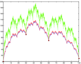
(a) $\sigma_{(r)}=\overline{112}$

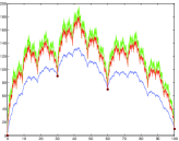
(b) $\sigma_{(r)}=\overline{221}$

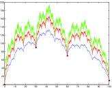
(c) $\sigma_{(r)}=\overline{12}$

$$\mbox{Blue Curve ({\color[rgb]{0,0,1}{---}}):}\ SFIFg_{\sigma_{(b)}}\ \mbox{for}\ \sigma_{(b)}=\bar{1}\ \mbox{in}(a),(b)\ \mbox{and}\ (c),$$

$$\mbox{Green Curve ({\color[rgb]{0,1,0}{---}}):}\ SFIFg_{\sigma_{(g)}}\ \mbox{for}\ \sigma_{(g)}=\bar{2}\ \mbox{in}(a),(b)\ \mbox{and}\ (c),$$

$$\mbox{Red Curve ({\color[rgb]{1,0,0}{---}}):}\ SFIFg_{\sigma_{(r)}}\ \mbox{for}\ \sigma_{(r)}=\overline{112}\ \mbox{in}(a),\ \mbox{for}\ \sigma_{(r)}=\overline{221}\ \mbox{in}\ (b)\ \mbox{and}\ \mbox{for}\ \sigma_{(r)}=\overline{12}\ \mbox{in}\ (c)$$

Figure 1: SFIFs for $\sigma_{(b)}=\bar{1}$, $\sigma_{(g)}=\bar{2}$ and different choices of $\sigma_{(r)}$

The SFIFs $g_{\sigma_{(b)}}\ \mbox{for}\ \sigma_{(b)}=\bar{1}$ and $g_{\sigma_{(g)}}\ \mbox{for}\ \sigma_{(g)}=\bar{2}$ are in fact FIFs (c.f. Figs. 1(a)- 1(c), blue and green curves ), since these are constructed with a single element of SIFS (2.5).

Heuristically, in terms of their fractal dimension [1], the graphs of SFIF $g_{\sigma_{(r)}}$ appear to fill more space in $\mathbb{R}^{2}$ than the graph of FIF $g_{\sigma_{(b)}}$ and less space in $\mathbb{R}^{2}$ than the graph of FIF $g_{\sigma_{(g)}}$. In fact, the fractal dimension of graphs of FIF $g_{\sigma_{(b)}}$ and $g_{\sigma_{(g)}}$ are computed as $1.3069$ and $1.5199$ respectively whereas the fractal dimension of SFIF $g_{\sigma_{(r)}}$ with $\sigma_{(r)}=\overline{112}$ (c.f. Fig. 1(a), red curve) is $1.3632$, the fractal dimension of SFIF $g_{\sigma_{(r)}}$ with $\sigma_{(r)}=\overline{221}$ (c.f. Fig. 1(b), red curve) is $1.4572$ and the fractal dimension of SFIF $g_{\sigma_{(r)}}$ with $\sigma_{(r)}=\overline{12}$ (c.f. Fig. 1(c), red curve) is $1.4182$.

Further, for FIFs $g_{\sigma_{(b)}}$ and $g_{\sigma_{(g)}}$, the average fractal distance defined as $\\ d_{F}(f,g)=\frac{1}{(b-a)}\left(\int\limits_{a}^{b}|f(x)-g(x)|^{2}dx\right)^{1/2}$ for the functions $f$ and $g$, continuous on a closed interval $[a,b]$, is $d_{F}(g_{\sigma_{(b)}},g_{\sigma_{(g)}})=0.297$. It is observed that (i) for SFIF $g_{\sigma_{(r)}}$ with $\sigma_{(r)}=\overline{112}$, $d_{F}(g_{\sigma_{(b)}},g_{\sigma_{(r)}})=0.022$ while $d_{F}(g_{\sigma_{(g)}},g_{\sigma_{(r)}})=0.276$. So, if the data generating function is at one third average fractal distance from FIF $g_{\sigma_{(b)}}$, then SFIF $g_{\sigma_{(r)}}$ is a better approximation of the data generating function, since $g_{\sigma_{(r)}}$ is closer to $g_{\sigma_{(b)}}$ than $g_{\sigma_{(g)}}$ (c.f. Fig. 1(a)) i.e. $d_{F}(g_{\sigma_{(b)}},g_{\sigma_{(r)}})<d_{F}(g_{\sigma_{(g)}},g_{\sigma_{(r)}})$. (ii) For SFIF $g_{\sigma_{(r)}}$ with $\sigma_{(r)}=\overline{221}$, $d_{F}(g_{\sigma_{(b)}},g_{\sigma_{(r)}})=0.228$ while $d_{F}(g_{\sigma_{(g)}},g_{\sigma_{(r)}})=0.071$. So, if the data generating function is at one third average fractal distance from FIF $g_{\sigma_{(g)}}$, then SFIF $g_{\sigma_{(r)}}$ is a better approximation of such data generating function, since $g_{\sigma_{(r)}}$ is closer to $g_{\sigma_{(g)}}$ than $g_{\sigma_{(b)}}$ (c.f. Fig. 1(b)) and (iii) for $g_{\sigma_{(r)}}$ with $\sigma_{(r)}=\overline{12}$, $d_{F}(g_{\sigma_{(b)}},g_{\sigma_{(r)}})=0.138$ and $d_{F}(g_{\sigma_{(g)}},g_{\sigma_{(r)}})=0.162$. So, if the data generating function lies in the middle of FIFs $g_{\sigma_{(b)}}$ and $g_{\sigma_{(g)}}$, then SFIF $g_{\sigma_{(r)}}$ (c.f. Fig. 1(c)) is a better approximation of such data generating function.

4 Integral and Derivative of SFIF

In this section, for a SFIF passing through a given interpolation data, its integral is shown to be also a SFIF, albeit for a different interpolation data. Further, in this section, the smoothness of SFIF is investigated in terms of its Lipschitz exponent and it is found that, in general, a SFIF may not be differentiable. This, as a natural follow up, led to determining in this section the conditions for existence of derivatives of a SFIF.

In order to study the integral of a SFIF, a SIFS

$$\Big{\{}\big{\{}\mathbb{R}^{2};\ \omega_{n,k}(x,y)=(L_{n}(x),G_{n,k}(x,y)):n=1,\ldots,N\big{\}},\ k=1,\ldots,M\Big{\}},$$ (4.1)

associated with the data $\{(x_{i},y_{i})\in\mathbb{R}^{2}:i=0,\ldots,N\}$ is considered, where $\ L_{n}(x)=a_{n}x+b_{n}$ are given by (2.2) and the functions $\ G_{n,k}(x,y)$ defined by

$$G_{n,k}(x,y)=\gamma_{n,k}y+q_{n,k}(x),\quad n=1,\ldots,N.$$ (4.2)

satisfy the join up conditions given by (2.4). Here, $\gamma_{n,k}$ are free parameters chosen such that $|\gamma_{n,k}|<1$ and $\gamma_{n,k}\neq\gamma_{n,l}$ for $k\neq l$ and $q_{n,k}(x)$ are affine functions. Condition (2.4) ensures that there exits a unique attractor $G_{\sigma}\in{\cal H}(\mathbb{R}^{2})$ of SIFS (4.1). By the arguments similar to those in the proof of Theorem 2.1, $G_{\sigma}$ is graph of a continuous function $g_{\sigma}$.

The following notations [4] are needed in the sequel for tidy presentation of our results:

$$\left.\begin{array}[]{ll}\hat{\gamma}_{n,k}&=a_{n}\gamma_{n,k}\\ \hat{y}_{N,k}&=\hat{y}_{0}+\frac{\sum\limits_{j=1}^{N}a_{j}\big{[}\int\limits_{x_{0}}^{x_{N}}q_{j,k}(t)\ dt\big{]}}{1-\sum\limits_{j=1}^{N}a_{j}\gamma_{j,k}}\\ \hat{y}_{n,k}&=\hat{y}_{0}+\sum\limits_{j=1}^{n}a_{j}\big{[}\gamma_{j,k}(\hat{y}_{N,k}-\hat{y}_{0})\ +\int\limits_{x_{0}}^{x_{N}}q_{j,k}(t)\ dt\big{]}\\ \hat{q}_{n,k}(x)&=\hat{y}_{n-1,k}-a_{n}\gamma_{n,k}\hat{y}_{0}+a_{n}\int\limits_{x_{0}}^{x}q_{n,k}(t)\ dt\end{array}\right\}$$ (4.7)

where, $\hat{y}_{0}$ is an arbitrary real number. To determine an interpolation data through which the integral of SFIF passes, let the affine functions $q_{n,k}(x)$ in (4.2) satisfy :

$$\frac{\sum\limits_{j=1}^{N}a_{j}\int\limits_{x_{0}}^{x_{N}}q_{j,k}}{1-\sum\limits_{j=1}^{N}a_{j}\gamma_{j,k}} =\frac{\sum\limits_{j=1}^{N}a_{j}\int\limits_{x_{0}}^{x_{N}}q_{j,l}}{1-\sum\limits_{j=1}^{N}a_{j}\gamma_{j,l}}\neq 1\quad\mbox{for }\ k\neq l,\ k,l=1,\ldots,M.$$ (4.8)

For example, for $a_{j}=\frac{1}{N}$, $\gamma_{j,k}=\gamma_{k}$ and $q_{j,k}=(1-\gamma_{k})(e_{j}x+f_{j})$ for $j=1,\ldots,N$, the condition (4.8) is satisfied. Then, $\hat{y}_{i,k}=\hat{y}_{i,l}=\hat{y}_{i}$ for $i=0,\ldots,N$; $k,l=1,\ldots,M$ and $\hat{y}_{N}-\hat{y}_{0}\neq 1$.

The SIFS associated with the data $\{(x_{i},\hat{y}_{i})\in\mathbb{R}^{2}:i=0,\ldots N\}$ is now defined as the pool of IFS

$$\Big{\{}\big{\{}\mathbb{R}^{2};\ \hat{\omega}_{n,k}(x,y)=(L_{n}(x),\hat{G}_{n,k}(x,y)):\ n=1,\ldots,N\big{\}},k=1,\ldots,M\Big{\}}$$ (4.9)

where, the functions

$$\hat{G}_{n,k}(x,y) =\hat{\gamma}_{n,k}y+\hat{q}_{n,k}(x)$$ (4.10)

satisfy the join-up conditions $\ \hat{G}_{n,k}(x_{0},\hat{y}_{0})=\hat{y}_{n-1}\$ and $\ \hat{G}_{n,k}(x_{N},\hat{y}_{N})=\hat{y}_{n}$. These join-up conditions ensure that there exits a unique attractor $\hat{G}_{\sigma}\in{\cal H}(\mathbb{R}^{2})$ of SIFS (4.9). The following theorem shows that the integral of SFIF is also a SFIF albeit for interpolation data $\{(x_{i},\hat{y}_{i})\in\mathbb{R}^{2}:i=0,\ldots N\}$.

Theorem 4.1

For the interpolation data $\{(x_{i},y_{i})\in\mathbb{R}^{2}:i=0,\ldots N\}$, let $g_{\sigma}$ be SFIF corresponding to SIFS (4.1) for $\sigma\in\Lambda$. Then, the integral

$$\hat{g}_{\sigma}(x)=\hat{y}_{0}+\int\limits_{x_{0}}^{x}g_{\sigma}(t)\ dt$$ (4.11)

is SFIF associated with SIFS (4.9) for the interpolation data $\{(x_{i},\hat{y}_{i}):i=0,\ldots,N\}$.

• Using (4.11) and (2.1), it is observed that,

  $$\hat{g}_{\sigma}(L_{i_{k}}\circ\ldots\circ L_{i_{1}}(x)) =\hat{g}_{\sigma}(L_{i_{k}}\circ\ldots\circ L_{i_{1}}(x_{0}))+\left(\prod\limits_{j=1}^{k}a_{i_{j}}\gamma_{i_{j},\sigma_{j}}\right)\Big{(}\hat{g}_{\sigma}(x)-\hat{y}_{0}\Big{)}$$

  $$\quad\mbox{}+\sum\limits_{p=1}^{k}\left(\prod\limits_{j=p+1}^{k}a_{i_{j}}\gamma_{i_{j},\sigma_{j}}\right)a_{i_{p}}\int\limits_{L_{i_{p-1}}\circ\ldots\circ L_{i_{1}}(x_{0})}^{L_{i_{p-1}}\circ\ldots\circ L_{i_{1}}(x)}q_{i_{p},\sigma_{p}}(t).$$ (4.12)

  Also, by (4.11),

  $$\hat{g}_{\sigma}(L_{i_{k}}\circ\ldots\circ L_{i_{1}}(x_{0})) =\hat{y}_{0}+\sum\limits_{p=1}^{k}\bigg{(}\prod\limits_{j=p+1}^{k}a_{i_{j}}\gamma_{i_{j},\sigma_{j}}\bigg{)}\bigg{\{}\sum\limits_{l=1}^{i_{p}-1}a_{l}\bigg{[}\gamma_{l,\sigma_{p}}(\hat{y}_{N}-\hat{y}_{0})$$

  $$\quad\mbox{}+\int\limits_{x_{0}}^{x_{N}}q_{l,\sigma_{p}}(t)\ dt\bigg{]}+a_{i_{p}}\int\limits_{x_{0}}^{L_{i_{p-1}}\circ\ldots\circ L_{i_{1}}(x_{0})}q_{i_{p},\sigma_{p}}(t)\bigg{\}}.$$

  The above identity and (4.7) give

  $$\hat{g}_{\sigma}(L_{i_{k}}\circ\ldots\circ L_{i_{1}}(x_{0}))$$

  $$=\bigg{(}\prod\limits_{j=1}^{k}a_{i_{j}}\gamma_{i_{j},\sigma_{j}}\bigg{)}\hat{y}_{0}$$

  $$\quad\mbox{}+\sum\limits_{p=1}^{k}\bigg{(}\prod\limits_{j=p+1}^{k}a_{i_{j}}\gamma_{i_{j},\sigma_{j}}\bigg{)}\bigg{\{}\hat{y}_{i_{p}-1}-a_{i_{p}}\gamma_{i_{p},\sigma_{p}}\ \hat{y}_{0}+a_{i_{p}}\int\limits_{x_{0}}^{L_{i_{p-1}}\circ\ldots\circ L_{i_{1}}(x_{0})}q_{i_{p},\sigma_{p}}(t)\bigg{\}}.$$ (4.13)

Now, substituting the value of $\hat{g}_{\sigma}(L_{i_{k}}\circ\ldots\circ L_{i_{1}}(x_{0}))$ from (Proof) in (Proof), it follows that

$$\hat{g}_{\sigma}(L_{i_{k}}\circ\ldots\circ L_{i_{1}}(x)) =\hat{G}_{i_{k},\sigma_{k}}\bigg{(}L_{i_{k-1}}\circ\ldots\circ L_{i_{1}}(x),\hat{G}_{i_{k-1},\sigma_{k-1}}\Big{(}.,\ldots$$

$$\quad\quad\quad\quad\hat{G}_{i_{2},\sigma_{2}}\big{(}L_{i_{1}}(x),\hat{G}_{i_{1},\sigma_{1}}(x,\hat{g}_{\sigma}(x))\big{)}\ldots\Big{)}\bigg{)}.$$

Thus, $\hat{g}_{\sigma}$ is SFIF associated with SIFS (4.9).  

Remark 4.1

In case of $\kappa$-SFIF $g_{\sigma,\kappa}$ (c.f. Remark 2.2), using the lines of proof of Theorem 4.1, it follows that the integral of $\kappa$-SFIF is not a $\kappa$-SFIF but integral of $g_{\sigma,\kappa}+\xi_{\sigma}$, where $\xi_{\sigma}$ is defined by

$$\xi_{\sigma}(x)=\gamma_{i_{n},\sigma_{n}}\left[\xi_{\sigma}(L_{n}^{-1}(x))-\kappa(1-L_{n}^{-1}(x))\right]+\kappa(1-x)$$ (4.14)

for $x\in I_{n}$, is a $\kappa$-SFIF for the interpolation data $\{(x_{i},\hat{y}_{i})\in\mathbb{R}^{2}:i=0,\ldots N\}$, provided

$$\frac{\sum\limits_{j=1}^{N}a_{j}[\int\limits_{x_{0}}^{x_{N}}(q_{j,k}(t)-\kappa\gamma_{j,k}(1-t))dt]}{1-\sum\limits_{j=1}^{N}a_{j}\gamma_{j,k}} =\frac{\sum\limits_{j=1}^{N}a_{j}[\int\limits_{x_{0}}^{x_{N}}(q_{j,l}(t)-\kappa\gamma_{j,l}(1-t))dt]}{1-\sum\limits_{j=1}^{N}a_{j}\gamma_{j,l}}\neq 1\quad\mbox{holds}.$$

Here, $\hat{y}_{j,k}$ , $\hat{q}_{j,k}(x),\ j=1,2,\ldots,N$, in (4.7) are given by

$$(1-\kappa)\hat{y}_{N,k} =\kappa(x_{0}-x_{N})+(1-\kappa)\hat{y}_{0}$$

$$\mbox{}+\frac{\sum\limits_{n=1}^{N}a_{n}\bigg{\{}\int\limits_{x_{0}}^{x_{N}}q_{n,k}(t)\ dt+\kappa\int\limits_{x_{0}}^{x_{N}}(1-L_{n}(t))\ dt-\kappa\ \gamma_{n,k}\int\limits_{x_{0}}^{x_{N}}(1-t)\ dt\bigg{\}}}{1-\sum\limits_{n=1}^{N}a_{n}\gamma_{n,k}}$$

$$(1-\kappa)\hat{y}_{j,k} =\kappa(x_{0}-x_{j})+(1-\kappa)\hat{y}_{0}+\sum\limits_{n=1}^{j}a_{n}\bigg{[}\gamma_{n,k}\bigg{\{}(1-\kappa)(\hat{y}_{N,k}-\hat{y}_{0})$$

$$\quad\mbox{}+\kappa\int\limits_{x_{0}}^{x_{N}}t\ dt\bigg{\}}+\int\limits_{x_{0}}^{x_{N}}\{\kappa(1-L_{n}(t))+q_{n,k}(t)\}\ dt\bigg{]}$$

and

$$\hat{q}_{j,k}(x) =\kappa x_{j-1}+(1-\kappa)\hat{y}_{j-1,k}-a_{j}\gamma_{j,k}\bigg{[}\kappa x_{0}+(1-\kappa)\hat{y}_{0}+\kappa\int\limits_{x_{0}}^{x}(1-t)\ dt\bigg{]}$$

$$\quad\mbox{}+a_{j}\kappa\int\limits_{x_{0}}^{x}(1-L_{j}(t))\ dt+a_{j}\int\limits_{x_{0}}^{x}q_{j,k}(t)\ dt.$$ (4.15)

For investigating the smoothness of a SFIF, the following notations are needed:

$$\lambda =\min\{\lambda_{n,k}:n=1,2,\ldots,N,\ k=1,2,\ldots M\},\mbox{where}\ \lambda_{n,k}\ \mbox{are real numbers}$$

$$\hskip 227.62204pt\mbox{ satisfying}\ 0<\lambda_{n,k}\leq 1$$

$$C_{1} =\max\{\frac{|\gamma_{n,k}|}{|I_{n}|^{\lambda}}:n=1,2,\ldots,N,\ k=1,2,\ldots,M\},\mbox{where}\ \gamma_{n,k}\ \mbox{are real numbers}$$

$$\hskip 227.62204pt\mbox{satisfying}\ |\gamma_{n,k}|\leq 1.$$

$$\mbox{Modulus of continuity of }\ g_{\sigma}(x)\ \mbox{as}\ \omega(g_{\sigma},t)=\max\limits_{|h|\leq t}\max\limits_{x}|g_{\sigma}(x+h)-g_{\sigma}(x)|$$ (4.16)

The smoothness of a SFIF in terms of its Lipscitz exponent is given by the following theorem:

Theorem 4.2

Let $g_{\sigma}$ be a SFIF corresponding to SIFS (4.1) with $q_{n,k}\in\mbox{Lip}\ \lambda_{n,k}$, $0<\lambda_{n,k}\leq 1$. Then,

1. for $C_{1}<1$, $\ g_{\sigma}\in Lip\ \lambda$

2. for $C_{1}=1$, $\ \omega(g_{\sigma},t)=O(|t|^{\lambda}\log|t|)$

3. for $C_{1}>1$, $\ g_{\sigma}\in Lip\ \bar{\lambda}$,

where, $\bar{\lambda}\leq\max\limits_{\begin{subarray}{c}n=1,\ldots,N\\ k=1,\ldots,M\end{subarray}}\left(\frac{\log\gamma_{n,k}}{\log a_{n}}\right)$ and $C_{1}$, $\lambda$ are given by (4).

• The method of proof is similar to that in [9], wherein $\gamma_{n}$ is replaced by $\gamma_{n,\sigma_{n}}$.  

Remark 4.2

It follows from Theorem 4.2 that $g_{\sigma}\in Lip\ \overline{\lambda_{k}}$ for $C_{1}\geq C_{1,k}>1$, where $C_{1,k}=\max\{\frac{|\gamma_{n,k}|}{|I_{n}|^{\lambda_{k}}}:n=1,2,\ldots,N\}$ and $\overline{\lambda_{k}}\leq\max\{\frac{\log|\gamma_{n,k}|}{\log|I_{n}|}:n=1,2,\ldots,N\}$.

Remark 4.3

In case of $\kappa$-SFIF $g_{\sigma,\kappa}$(c.f. Remark 2.2), the smoothness result analogous to Theorem 4.2 can be obtained as follows: (i) $g_{\sigma,\kappa}\in Lip\ \lambda$ for $C_{1}<1$, (ii) $\ \omega(g_{\sigma,\kappa},t)=O(|t|^{\lambda}\log|t|)$ for $C_{1}=1$ and (iii) $g_{\sigma,\kappa}\in Lip\ \bar{\lambda}$ for $C_{1}>1$, $\bar{\lambda}\leq\max\{(\log\gamma_{n,k})/(\log a_{n}):n=1,2,\ldots,N,\ k=1,2,\ldots,M\}$.

In general, a SFIF belonging to certain Lipschitz class, need not be differentiable. This, as a natural follow up, leads to identification of conditions for the existence of derivative of a SFIF in the following proposition:

Proposition 4.1

For the interpolation data $\{(x_{i},y_{i})\in\mathbb{R}^{2}:i=0,1,\ldots N\}$, let $g_{\sigma}$ be a SFIF corresponding to SIFS (4.1) for $\sigma\in\Lambda$. Then, $\hat{g}_{\sigma}^{\prime}$ exists and $\hat{g}_{\sigma}^{\prime}(x)=g_{\sigma}(x)$ if and only if $\ \hat{g}_{\sigma}$ is a SFIF associated with SIFS (4.9) for the interpolation data $\{(x_{i},\hat{y}_{i}):i=0,1,\ldots,N\}$, provided $\hat{\gamma}_{j,k}=a_{j}\gamma_{j,k}$ and $\frac{d}{dx}(\hat{q}_{j,k}(x))=a_{j}q_{j,k}(x)$ hold.

• If $\ \hat{g}_{\sigma}^{\prime}(x)=g_{\sigma}(x)$, then $\ \hat{g}_{\sigma}(x)=\hat{y}_{0}+\int\limits_{x_{0}}^{x}g_{\sigma}(t)\ dt$, so that “ if ” part follows from Theorem 4.1. Conversely, suppose $\ \hat{g}_{\sigma}\$ is a SFIF associated with SIFS (4.9) for the interpolation data $\{(x_{i},\hat{y}_{i}):i=0,\ldots,N\}$. Then,

  $$\hat{g}_{\sigma}(L_{i_{k}}\circ\ldots\circ L_{i_{1}}(x)) =\left(\prod\limits_{j=1}^{k}\hat{\gamma}_{i_{j},\sigma_{j}}\right)\hat{g}_{\sigma}(x)$$

  $$\quad\mbox{}+\sum\limits_{p=1}^{k}\left(\prod\limits_{j=p+1}^{k}\hat{\gamma}_{i_{j},\sigma_{j}}\right)\hat{q}_{i_{p},\sigma_{p}}(L_{i_{p-1}}\circ\ldots\circ L_{i_{1}}(x)).$$ (4.17)

  Since, $\frac{d}{dx}(\hat{q}_{j,k}(x))=a_{j}q_{j,k}(x)$

  $$\hat{q}_{j,k}(x) =\hat{q}_{j,k}(x_{0})+a_{j}\int\limits_{x_{0}}^{x}q_{j,k}(t)dt=\hat{y}_{j-1}-a_{j}\gamma_{j,k}\hat{y}_{0}+a_{j}\int\limits_{x_{0}}^{x}q_{j,k}(t)dt.$$ (4.18)

  Substituting (4.18) and $\hat{\gamma}_{j,k}=a_{j}\gamma_{j,k}$ in (Proof),

  $$\hat{g}_{\sigma}(L_{i_{k}}\circ\ldots\circ L_{i_{1}}(x)) =\Big{(}\prod\limits_{j=1}^{k}a_{i_{j}}\gamma_{i_{j},\sigma_{j}}\Big{)}\hat{g}_{\sigma}(x)+\sum\limits_{p=1}^{k}\Big{(}\prod\limits_{j=p+1}^{k}a_{i_{j}}\gamma_{i_{j},\sigma_{j}}\Big{)}\times$$

  $$\quad\mbox{}\times\Big{[}\hat{y}_{i_{p}-1}-a_{i_{p}}\gamma_{i_{p},\sigma_{p}}\hat{y}_{0}+a_{i_{p}}\int\limits_{x_{0}}^{L_{i_{p-1}}\circ\ldots\circ L_{i_{1}}(x)}q_{i_{p},\sigma_{p}}(t)dt\Big{]}.$$ (4.19)

  For a fixed $\sigma\in\Lambda$, it is easily seen that the Read-Bajraktarevic operator $\hat{T}$ defined by

  $$\hat{T}(\sigma,g)(x) =\lim\limits_{k\rightarrow\infty}\bigg{\{}\Big{(}\prod\limits_{j=1}^{k}a_{i_{j}}\gamma_{i_{j},\sigma_{j}}\Big{)}g(L_{i_{1}}^{-1}\circ\ldots\circ L_{i_{k}}^{-1}(x))+\sum\limits_{p=1}^{k}\Big{(}\prod\limits_{j=p+1}^{k}a_{i_{j}}\gamma_{i_{j},\sigma_{j}}\Big{)}\times$$

  $$\quad\mbox{}\times\Big{[}\hat{y}_{i_{p}-1}-a_{i_{p}}\gamma_{i_{p},\sigma_{p}}\hat{y}_{0}+a_{i_{p}}\int\limits_{x_{0}}^{L_{i_{p}}^{-1}\circ\ldots\circ L_{i_{k}}^{-1}(x)}q_{i_{p},\sigma_{p}}(t)dt\Big{]}\bigg{\}}$$ (4.20)

  is a contraction map on ${\cal\hat{G}}=\{f:I\rightarrow\mathbb{R}\ \ \mbox{such that}\ f\ \mbox{ is continuous},\ f(x_{0})=\hat{y}_{0}\ \mbox{and}\\ f(x_{N})=\hat{y}_{N}\}$. By (Proof), the function $\hat{g}_{\sigma}$ is a fixed point of $\hat{T}$. Also, by Theorem 4.1, the function $h(x)=\hat{y}_{0}+\int\limits_{x_{0}}^{x}g_{\sigma}(t)\ dt\$ is a SFIF associated with SIFS (4.9) satisfying (Proof). Consequently, $h$ also is a fixed point of $\hat{T}$. Hence, by uniqueness of fixed point of Read-Bajraktarevic operator $\hat{T}$, $\ \hat{g}_{\sigma}(x)=\hat{y}_{0}+\int\limits_{x_{0}}^{x}g_{\sigma}(t)\ dt\$ which implies that $\hat{g}_{\sigma}^{\prime}$ exists and $\hat{g}_{\sigma}^{\prime}(x)=g_{\sigma}(x)$, since $g_{\sigma}$ being a SFIF corresponding to SIFS (4.1), is a continuous function.  

For the investigation of $n^{th}$ derivative of SFIF, denote

$$G_{i,k,j}(x,y)=\gamma_{i,k,j}\ y+q_{i,k,j}(x)$$ (4.21)

where, $G_{i,k,0}(x,y)=G_{i,k}(x,y)$, $\ q_{i,k,0}(x)=q_{i,k}(x)$, $\ \gamma_{i,k,0}=\gamma_{i,k}\$ and $\ G_{i-1,k,j}(x_{N},y_{N,k,j})=G_{i,k,j}(x_{0},y_{0,k,j})$, $\ i=1,\ldots,N,\ k=1,\ldots,M\ \mbox{and}\ j=0,1,\ldots,n$. To determine interpolation data through which derivatives of SFIF passes, let the affine maps $q_{i,k,j}(x)$ in (4.21) satisfy :

$$\frac{\sum\limits_{p=1}^{N}a_{p}\int\limits_{x_{0}}^{x_{N}}q_{p,k,j}}{1-\sum\limits_{p=1}^{N}a_{p}\gamma_{p,k,j}}=\frac{\sum\limits_{p=1}^{N}a_{p}\int\limits_{x_{0}}^{x_{N}}q_{p,l,j}}{1-\sum\limits_{p=1}^{N}a_{p}\gamma_{p,l,j}}\neq 1,$$ (4.22)

where $\hat{y}_{0,j},j=0,1,\ldots,n$ are arbitrary real numbers. For example, for $a_{i}=\frac{1}{N}$, $\gamma_{i,k,j}=\gamma_{k,j}$ and $q_{i,k,j}=(1-\gamma_{k})\bar{q}_{i,j}(x)$, where $\bar{q}_{i,j}(x)$ are polynomials of degree $n-j$ for $i=1,\ldots,N$, the condition (4.22) is satisfied. Then, $\hat{y}_{i,k,j}=\hat{y}_{i,l,j}=\hat{y}_{i,j}$ for $i=1,\ldots,N$, $k,l=1,\ldots,M$ and $j=0,1,\ldots,n$.

The SIFS associated with the interpolation data $\{(x_{i},y_{i,j}):i=0,1,\ldots,N\}$, $j=0,1,\ldots,n$, is now defined as

$$\Big{\{}\big{\{}\mathbb{R}^{2};\ \omega_{i,k,j}(x,y)=(L_{i}(x),G_{i,k,j}(x,y)):i=1,\ldots,N\big{\}},\ k=1,\ldots,M\Big{\}}.$$ (4.23)

It is observed that SIFS (4.23) reduces to SIFS (4.1) if $j=0$. The following theorem gives the existence of derivatives of a SFIF.

Theorem 4.3

Let the functions $G_{i,k,j}(x,y)$ defined in (4.21) be such that, for some integer $n\geq~{}0$, $|\gamma_{i,k}|<a_{i}^{n}$, $\ q_{i,k}\in C^{n}[x_{0},x_{N}],\ i=1,2,\ldots,N,\ k=1,2,\ldots,M$ and $g_{\sigma}$ be a SFIF corresponding to SIFS (4.23) for $j=0$ and $\sigma\in\Lambda$. Then, for $j=1,2,\ldots,n$, $g_{\sigma}^{(j)}$ exists and is a SFIF associated with SIFS (4.23) for the interpolation data $\{(x_{i},y_{i,j}):i=0,1,\ldots,N\}$, provided $\gamma_{i,k,j}=\frac{\gamma_{i,k}}{a_{i}^{j}}\$ and $\ q_{i,k,j}(x)=\frac{q_{i,k,j-1}^{(1)}(x)}{a_{i}}$.

• The equation $G_{1,k,j}\left(x_{0},y_{0,j}\right)=y_{0,j}\$ gives $\ y_{0,j}=\frac{\gamma_{1,k}}{a_{1}^{j}}y_{0,j}+\frac{q_{1,k}^{(j)}(x_{0})}{a_{1}^{j}}\$ which implies $\\ y_{0,j}=\frac{q_{1,k}^{(j)}(x_{0})}{(a_{1}^{j}-\gamma_{1,k})}$. Similarly, $\ G_{N,k,j}\left(x_{N},y_{N,j}\right)=y_{N,j}\$ gives $y_{N,j}=\frac{q_{N,k}^{(j)}(x_{N})}{(a_{N}^{j}-\gamma_{N,k})}$. By Proposition 4.1, it now follows that, for $j=1,2,\ldots,n$, $g_{\sigma}^{(j)}(x)$ is the SFIF associated with SIFS $\Big{\{}\big{\{}\mathbb{R}^{2};\ \omega_{i,k,j}(x,y)=(L_{i}(x),G_{i,k,j}(x,y)):i=1,2,\ldots,N\big{\}},\ k=1,2,\ldots,M\Big{\}}$.  

Remark 4.4

In the case of $\kappa$-SFIF, Remark 4.1 and Theorem 4.3 suggest that the function $\tilde{g}_{\sigma,\kappa}^{(j)}=g_{\sigma,\kappa}^{(j)}(x)-\sum\limits_{p=1}^{j}\xi_{\sigma}^{(p-1)}(x)$, with $\xi_{\sigma}$ given by (4.14), is $\kappa$-SFIF associated with the SIFS

$$\Big{\{}\big{\{}\mathbb{R}^{2};\ \omega_{i,k,j}:i=1,2,\ldots,N\big{\}},\ k=1,2,\ldots,M\Big{\}},j=0,1,\ldots,n.$$

Using (4.14) and (4.1), it is easily seen that $\ y_{0,1}=\frac{q_{1,k}^{(1)}(x_{0})}{(1-\kappa)(a_{1}-\gamma_{1,k})}-\frac{\kappa}{1-\kappa}\$ and $\\ y_{N,k,1}=\frac{q_{N,k}^{(1)}(x_{N})}{(1-\kappa)(a_{N}-\gamma_{N,k})}-\frac{\kappa}{1-\kappa}$. Also, $\ y_{0,j}=\frac{q_{1,k}^{(j)}(x_{0})}{(1-\kappa)(a_{1}^{j}-\gamma_{1,k})}\quad\mbox{and}\ y_{N,k,j}=\frac{q_{N,k}^{(j)}(x_{N})}{(1-\kappa)(a_{N}^{j}-\gamma_{N,k})}$,
$k=1,2,\ldots,M$, for $j>1$.

5 Conclusions

In the present work, the notion of Super Fractal Interpolation Function (SFIF) is introduced for finer simulation of the objects of the nature or outcomes of scientific experiments that reveal one or more structures embedded in to another. Since, in the construction of SFIF, at each level of iteration, an IFS can be chosen from a pool of several IFS, the desired randomness and variability can be implemented in fractal interpolation of the given data. Thus, SFIF may be used as a tool for better geometrical modeling of objects found in nature and results of certain scientific experiments. Also, an expository description of investigations on the integral, the smoothness and determination of conditions for existence of derivatives of a SFIF is given in the present work. It is proved that, for a SFIF passing through a given interpolation data, its integral is also a SFIF, albeit for a different interpolation data. The smoothness of a SFIF is given in terms of its Lipschitz exponent. A SFIF $g_{\sigma}$, for $C_{1}\neq 1$, belongs to a Lipschitz class and, for $C_{1}=1$, $\ \omega(g_{\sigma},t)=O(|t|^{\lambda}\log|t|)$. It is seen that the smoothness of SFIF depend on free variables $\gamma_{n,k}$ as well as on the smoothness of affine functions $q_{n,k}(x)$ occurring in its definition. Further, sufficient conditions for existence of derivatives of a SFIF are derived in the present paper. Our results on SFIF found here are likely to have wide applications in areas like pattern-forming alloy solidification in chemistry, blood vessel patterns in biology, signal processing, fragmentation of thin plates in engineering, stock markets in finance, wherein significant randomness and variability is observed in simulation of various processes.

References

[1]
Barnsley M.F.
Fractal functions and interpolation.
Constructive Approximation, 2:303–329, 1986.
[2]
Barnsley M.F.
Fractals Everywhere.
Academic Press, Orlando, Florida, 1988.
[3]
Barnsley M.F.
Super Fractals.
Cambridge University Press, 2006.
[4]
Barnsley M.F. and Harrington A.N.
The calculus of fractal interpolation functions.
Journal of Approximation Theory, 57:14–34, 1989.
[5]
Barnsley M.F., Hutchinson J.E., and Stenflo O.
A fractal valued random iteration algorithm and fractal hierarchy.
Fractals, 13(2):111–146, 2005.
[6]
Barnsley M.F., Hutchinson J.E., and Stenflo O.
V-variable fractals: Fractals with partial self similarity.
Advances in Mathematics, 218:2051–2088, 2008.
[7]
Dalla L., Drakopoulos V., and Prodromou M.
On the box dimension for a class of non-affine fractal interpolation
functions.
Analysis in Theory and Applications, 19(3):220–233, 2003.
[8]
Donovan G.C., Geronimo J.S., Hardin D.P., and Massopust P.R.
Construction of orthogonal wavelets using fractal interpolation
function.
SIAM Journal on Mathematical Analysis, 27(4):1158–1192, 1996.
[9]
Gang C.
The smoothness and dimension of fractal interpolation function.
Applied Mathematics - A Journal of Chinese Universities: Series
B, 11:409–428, 1996.
[10]
Guo W., Jiang J., and Qiao L.
Parametrization of balanced multiwavelet.
Analysis in Theory and Applications, 26(4):383–400, 2010.
[11]
Liang Y. and Su W.
Connection between the order of fractional calculus and fractional
dimensions of a type of fractal functions.
Analysis in Theory and Applications, 23(4):354–362, 2007.
[12]
Massopust P.
Interpolation and Approximation with Splines and Fractals.
Oxford University Press, 2010.
[13]
Yanyan L. and Jun W.
Dimensions for random self-conformal sets.
Analysis in Theory and Applications, 19(3):342–354, 2003.
[14]
Yong T. and Guangjun Y.
Construction of some kiesswetter-like functions -the continuous but
non-different-iable function defined by quinary decimal.
Analysis in Theory and Applications, 20(1):58–68, 2004.