Piezoelectric resonance in Rochelle salt: the contribution of diagonal strains

Abstract

Within the framework of two-sublattice Mitsui model with taking into account the shear strain $\varepsilon_{4}$ and the diagonal strains $\varepsilon_{2}$ and $\varepsilon_{3}$, a dynamic dielectric response of Rochelle salt X-cuts is considered. Experimentally observed phenomena of crystal clamping by high frequency electric field, piezoelectric resonance and microwave dispersion are described. It is shown that the lowest resonant frequency is always associated with the $\varepsilon_{4}$ shear mode

1 Introduction

Crystals of Rochelle salt have been attracting an interest of physicists due to their practical applications in past, and now from the fundamental point of view mostly. In contrast to most of the known ferroelectrics, in Rochelle salt the ferroelectric phase exists only in a temperature interval between two second order phase transitions at 255 and 297 K. Spontaneous polarization $P_{1}$ is accompanied by shear strain $\varepsilon_{4}$. The ferroelectric phase is monoclinic (P$2_{1}11$); both paraelectric phases are orthorhombic (P$2_{1}2_{1}2_{1}$); all phases are non-centrosymmetric and piezoelectric.

Dynamical dielectric response of Rochelle salt exhibits several dispersion regions. Those are related to the domain wall motion [1, 2, 3] (below 1 kHz), piezoelectric resonance [3, 4, 6] (between 10 kHz and 10 MHz), microwave relaxation [7], and the submillimeter (100-700 GHz) resonances [8]. While the very low and very high frequency dispersions are relatively well studied, the presence of the piezoelectric resonance dispersion in Rochelle salt is acknowledged at best. Quantitative data is available mostly for the temperature dependence of the first resonance frequency [4, 5, 6], whereas very little information has been obtained [4] about details of the temperature or frequency dependence of the dielectric permittivity, mode assignment for different crystal cuts, etc.

Behavior of Rochelle salt is usually described within a two-sublattice Ising model with an asymmetric double-well potential (Mitsui model [9, 10, 11]). The pseudospin dynamics is considered within the Bloch equations or Glauber approach methods.

Rochelle salt is a perfect example of a system, whose dynamic dielectric response cannot be correctly described without taking into account the deformational effects. Their influence is revealed, in particular, in the phenomena of piezoelectric resonance and crystal clamping by a high-frequency measuring field, none of which can be obtained within theories based on underformable versions of the Mitsui model [10, 12]. Such theories yield a diverging relaxation time at the Curie point and, as a result, incorrect temperature behavior of the microwave permittivity near the phase transitions.

In [13] the dynamic dielectric permittivity of Rochelle salt has been calculated, using the model with piezoelectric coupling [14] with the shear strain $\varepsilon_{4}$, for the entire frequency range from the static limit (in the ferroelectric phase from about 1 kHz) to 10¹¹ Hz, including the piezoelectric resonance region. For a coupled dynamics of the shear strain $\varepsilon_{4}$ – pseudospin system, the standard methods of description of the lattice strain dynamics [5] based on Newtonian equations of motion has been combined with the Glauber approach to pseudospin dynamics. Evolution of the dielectric permittivity from the static free crystal value via the piezoelectric resonances to the clamped crystal value and to the microwave relaxation has been described. Recently, in [15] it has been pointed out that boundary conditions in [13] were not set correctly, which resulted in the underestimated values of the resonant frequencies; a correct equation for the resonant frequencies related to the shear $\varepsilon_{4}$ mode has been obtained [15].

In the paraelectric phases in Rochelle salt the longitudinal field $E_{1}$ excites only the shear mode $\varepsilon_{4}$, as $d_{14}$ is there the only non-zero piezoelectric coefficient associated with $E_{1}$. However, in the ferroelectric phase it can also excite the extensional modes associated with the diagonal strains $\varepsilon_{1}$, $\varepsilon_{2}$, and $\varepsilon_{3}$ via the non-zero coefficients $d_{11}$, $d_{12}$, $d_{13}$. The contributions of the extensional modes to the dielectric permittivity of Rochelle salt at frequencies far from the piezoelectric resonance region are not expected to be crucial, due to smallness of $d_{1i}$ ($i=1,2,3$) in comparison with $d_{14}$. The presence of these modes, however, changes the permittivity in the resonance region, at least giving rise to additional resonance peaks, and this should be explored.

In this paper we follow the same approach that has been used previously [13] for the case with only one shear mode. The modification of the Mitsui model of [16] that takes into account both the shear strain $\varepsilon_{4}$ and the diagonal strains is exploited. The drawbacks of the previous calculations related to setting the boundary conditions are removed. The expression for the dynamic dielectric permittivity and equations for the resonant frequencies of Rochelle salt X-cuts is obtained.

2 System thermodynamics in presence of diagonal strains

For the sake of the reader’s convenience, we shall present here the expressions for the related to the shear strain $\varepsilon_{4}$ thermodynamic and physical characteristics of Rochelle salt obtained within the modified two-sublattice Mitsui model with the shear strain $\varepsilon_{4}$ and with the diagonal strains [16].

The system behavior is described in terms of the following linear combinations of the mean values of the pseudospins belonging to different sublattices

$$\xi=\frac{1}{2}(\langle\sigma_{q1}\rangle+\langle\sigma_{q2}\rangle),\quad\sigma=\frac{1}{2}(\langle\sigma_{q1}\rangle-\langle\sigma_{q2}\rangle);$$

$\xi$ is the parameter of ferroelectric ordering in the system.

The thermodynamic potential of the model [16] within the mean field approximation reads

$$g_{2E}(T)=U_{seed}+\frac{J+K}{4}\xi^{2}+\frac{J-K}{4}\sigma^{2}-\frac{2\ln 2}{\beta}-\frac{1}{\beta}\ln\cosh\frac{\gamma+\delta}{2}\cosh\frac{\gamma-\delta}{2},$$ (1)

where ${U_{seed}}$ is the phenomenological part of the thermodynamical potential, representing the energy of the host lattice of heavy ions which forms the asymmetric double-well potentials for the pseudospins (see [16]); $\beta=1/k_{B}T$, $k_{B}$ is the Boltzmann constant, and

$$\gamma=\beta\left(\frac{J+K}{2}\xi-2\psi_{4}\varepsilon_{4}+\mu_{1}E_{1}\right),\quad\delta=\beta\left(\frac{J-K}{2}\sigma+\Delta\right).$$

Here $\mu_{1}$ is the effective dipole moment. The model parameter $\psi_{4}$ describes the internal field created by the piezoelectric coupling with $\varepsilon_{4}$. It is assumed that a longitudinal electric field $E_{1}$ is applied.

The parameters $J$, $K$ are the Fourier-transforms (at ${\bf k}=0$) of the constants of interaction between pseudospins belonging to the same and to different sublattices, respectively. They, along with the double well potential asymmetry parameter $\Delta$, are assumed [16] to be linear functions of the diagonal strains

$$J\pm K=J_{0}\pm K_{0}+2\sum\limits_{i=1}^{3}{\psi_{i}^{\pm}\varepsilon_{i}},\quad\Delta=\Delta_{0}+\sum\limits_{i=1}^{3}{\psi_{3i}\varepsilon_{i}}.$$ (2)

The stress-strain relations and polarization have been obtained in the following form [16]

$$\sigma_{i}=\sum\limits_{j=1}^{3}c_{ij}^{E0}[\varepsilon_{j}-\alpha_{j}^{0}(T-T_{j}^{0})]-\frac{1}{2v}\psi_{i}^{+}\xi^{2}-\frac{1}{2v}\psi_{i}^{-}\sigma^{2}-\frac{1}{v}\psi_{3i}\sigma,\quad({i}=1-3)$$

$$\sigma_{4}=c_{44}^{E0}\varepsilon_{4}-e_{14}^{0}E_{1}+2\frac{\psi_{4}}{v}\xi,$$ (3)

$$P_{1}=e_{14}^{0}\varepsilon_{4}+\chi_{11}^{\varepsilon 0}E_{1}+\frac{\mu_{1}}{v}\xi.$$ (4)

$\sigma_{i}$ are the components of the stress tensor in Voigt notations; $c_{ij}^{E0}$ are the “seed” elastic constants; $\alpha_{i}^{0}$ are the “seed” thermal expansion coefficients.

3 Vibrations of X-cuts of Rochelle salt

We consider vibrations of a thin rectangular $L_{y}\times L_{z}$ plate of a Rochelle salt crystal cut in the (100) plane (X-cut) induced by time-dependent electric field $E_{1}=E_{1t}\exp(i\omega t)$. This field gives rise to the shear strain $\varepsilon_{4}$ at all temperatures, as well as to the diagonal strains $\varepsilon_{1}$, $\varepsilon_{2}$, $\varepsilon_{3}$ in the ferroelectric phase. We take into account the in-plane vibrational modes, allowed by the system symmetry, and neglect the out-of-plane mode associated with $\varepsilon_{1}$.

Dynamics of the pseudospin subsystem will be described within the Glauber approach [17], where the kinetic equations for the time-dependent averages $\xi$ and $\sigma$ have the form [14]

$$-\alpha\frac{d}{dt}\xi=\xi-\frac{1}{2}[\tanh\frac{1}{2}(\gamma+\delta)+\tanh\frac{1}{2}(\gamma-\delta)],$$

$$-\alpha\frac{d}{dt}\sigma=\sigma-\frac{1}{2}[\tanh\frac{1}{2}(\gamma+\delta)-\tanh\frac{1}{2}(\gamma-\delta)].$$ (5)

Here $\alpha$ is the parameter setting the scale of the dynamic processes in the pseudospin subsystem. The form of (5) is not affected by inclusion of the diagonal strains into consideration.

Dynamics of the strains will be described by the standard method, using classical (Newtonian) equations of motion [18] of an elementary volume

$$\rho\frac{\partial^{2}\eta_{i}}{\partial t^{2}}=\sum_{k}\frac{\partial\sigma_{ik}}{\partial x_{k}},$$ (6)

where $\rho=1.767$ g/cm³ is the crystal density, $\eta_{i}$ are the displacements of an elementary volume along the axis $x_{i}$, $\sigma_{ik}$ are components of the the mechanical stress tensor. Relevant to our case are the displacements $\eta_{2}$ and $\eta_{3}$, giving the strains

$$\varepsilon_{2}=\frac{\partial\eta_{2}}{\partial y},\quad\varepsilon_{3}=\frac{\partial\eta_{3}}{\partial z},\quad\varepsilon_{4}=\frac{\partial\eta_{2}}{\partial z}+\frac{\partial\eta_{3}}{\partial y}.$$

At small deviations from the equilibrium the dynamic variables $\xi$, $\sigma$, and $\varepsilon_{j}$ (or $\eta_{i}$) can be presented as sums of the equilibrium values and of the fluctuational deviations, while the deviations are taken to be in the form of harmonic waves

$$\xi=\tilde{\xi}+\xi_{t}(y,z)\exp(i\omega t),\quad\sigma=\tilde{\sigma}+\sigma_{t}(y,z)\exp(i\omega t),\quad\eta_{i}=\tilde{\eta}_{i}+\eta_{it}(y,z)\exp(i\omega t).$$

Equations (2)-(4), (5), and (6) can be expanded in terms of these deviations up to the linear terms. For $\tilde{\xi}$ and $\tilde{\sigma}$ we obtain the same equations that follow from the condition of the thermodynamic potential (1) extremum [16].

From (2)-(4) we get the following constitutive equations

$$\sigma_{i}(y,z)=\sum\limits_{j=1}^{3}c_{ij}^{E0}\varepsilon_{jt}(y,z)-\frac{1}{v}\psi_{i}^{+}\tilde{\xi}\xi_{t}(y,z)-\frac{1}{v}\psi_{i}^{-}\tilde{\sigma}\sigma_{t}(y,z)-\frac{1}{v}\psi_{3i}\sigma_{t}(y,z),$$

$$\sigma_{4}(y,z)=c_{44}^{E0}\varepsilon_{4t}(y,z)-e_{14}^{0}E_{1t}+2\frac{\psi_{4}}{v}\xi_{t}(y,z),$$ (7)

$$P_{1t}(y,z)=e_{14}^{0}\varepsilon_{4t}(y,z)+\chi_{11}^{\varepsilon 0}E_{1t}+\frac{\mu_{1}}{v}\xi_{t}(y,z).$$ (8)

(for $i=1-3$). Taking these into into account, from (5), and (6) we get the following system of equations

$$-\alpha\frac{d}{dt}\xi_{t}+a_{1}\xi_{t}+a_{2}\sigma_{t}+a_{32}\varepsilon_{2t}+a_{33}\varepsilon_{3t}+a_{34}\varepsilon_{4t}=a_{02}E_{1t},$$

$$-\alpha\frac{d}{dt}\sigma_{t}+b_{1}\xi_{t}+b_{2}\sigma_{t}+b_{32}\varepsilon_{2t}+b_{33}\varepsilon_{3t}+b_{34}\varepsilon_{4t}=b_{02}E_{1t},$$

$$\rho\frac{\partial^{2}\eta_{2t}}{\partial t^{2}}=c_{22}^{E0}\frac{\partial^{2}\eta_{2t}}{\partial y^{2}}+c_{23}^{E0}\frac{\partial^{2}\eta_{2t}}{\partial y\partial z}+c_{44}^{E0}(\frac{\partial^{2}\eta_{2t}}{\partial z^{2}}+\frac{\partial^{2}\eta_{3t}}{\partial y\partial z})+$$

$$\quad{}+\frac{2\psi_{4}}{v}\frac{\partial\xi_{t}}{\partial z}-\frac{1}{v}[\psi^{+}_{2}\tilde{\xi}\frac{\partial\xi_{t}}{\partial y}+(\psi_{2}^{-}\tilde{\sigma}+\psi_{32})\frac{\partial\sigma_{t}}{\partial y}],$$

$$\rho\frac{\partial^{2}\eta_{3t}}{\partial t^{2}}=c_{23}^{E0}\frac{\partial^{2}\eta_{2t}}{\partial y\partial z}+c_{33}^{E0}\frac{\partial^{2}\eta_{3t}}{\partial z^{2}}+c_{44}^{E0}(\frac{\partial^{2}\eta_{3t}}{\partial y^{2}}+\frac{\partial^{2}\eta_{2t}}{\partial y\partial z})+$$ (9)

$$\quad{}+\frac{2\psi_{4}}{v}\frac{\partial\xi_{t}}{\partial y}-\frac{1}{v}[\psi^{+}_{3}\tilde{\xi}\frac{\partial\xi_{t}}{\partial y}+(\psi_{3}^{-}\tilde{\sigma}+\psi_{33})\frac{\partial\sigma_{t}}{\partial z}],$$

with

$$a_{1}=-1+\beta\frac{J+K}{4}\lambda_{1},\quad a_{2}=\beta\frac{K-J}{4}\lambda_{2},$$

$$a_{32,3}=\frac{\beta}{2}[\tilde{\xi}\lambda_{1}\psi^{+}_{2,3}-\lambda_{2}(\psi^{-}_{2,3}\tilde{\sigma}+\psi_{32,3})],\quad a_{34}=-\beta\psi_{4}\lambda_{1},\quad a_{02}=-\frac{\beta\mu_{1}}{2}\lambda_{1},$$

$$b_{1}=-\beta\frac{J+K}{4}\lambda_{2},\quad b_{2}=-1+\beta\frac{J-K}{4}\lambda_{2},\quad$$

$$b_{32,3}=-\frac{\beta}{2}[\tilde{\xi}\lambda_{2}\psi^{+}_{2,3}-\lambda_{1}(\psi^{-}_{2,3}\tilde{\sigma}+\psi_{32,3})],\quad b_{34}=\beta\psi_{4}\lambda_{2},\quad b_{02}=\frac{\beta\mu_{1}}{2}\lambda_{2}.$$

(Hereafter it is implied that the deviations are functions of $y$ and $z$.) We introduced the following notations

$$\lambda_{1}=1-\xi^{2}-\sigma^{2},\quad\lambda_{2}=2\xi\sigma.$$

Solving the two first equations of (9) with respect to $\xi_{t}$ at $\eta_{2t}=\eta_{3t}=0$ (regime of a mechanically clamped crystal), substituting the result into (8), and differentiating that with respect to the field, we find the dynamic dielectric permittivity of a clamped crystal

$$\varepsilon_{11}^{\varepsilon}(\omega)=\varepsilon_{11}^{\varepsilon 0}+4\pi\frac{\beta\mu_{1}^{2}}{2v}F_{1}(\alpha\omega),\quad\varepsilon_{11}^{\varepsilon 0}=1+4\pi\chi_{11}^{\varepsilon 0}.$$ (10)

where

$$F_{1}(\alpha\omega)=\frac{i\alpha\omega\lambda_{1}+\varphi_{3}}{(i\alpha\omega)^{2}+(i\alpha\omega)\varphi_{1}+\varphi_{2}},\quad\varphi_{1}=2-\frac{\beta J}{2}\lambda_{1},$$

$$\varphi_{2}=1-\frac{\beta J}{2}\lambda_{1}-\beta^{2}\frac{K^{2}-J^{2}}{16}(\lambda_{1}^{2}-\lambda_{2}^{2}),\quad\varphi_{3}=\lambda_{1}+\frac{\beta(K-J)}{4}(\lambda_{1}^{2}-\lambda_{2}^{2}).$$

This is the same expression that has been obtained previously [13] for the Mitsui model with the shear strain $\varepsilon_{4}$, but without the diagonal strains.

In the regime of a mechanically free crystal, the two first equations of (9) give

$$\xi_{t}(y,z)=\frac{\beta\mu_{1}}{2}F_{1}(\alpha\omega)E_{1t}-\beta\psi_{4}F_{1}(\alpha\omega)\varepsilon_{4t}(y,z)-$$

$$\quad{}-\frac{\beta}{2}F_{42}^{\xi}(\alpha\omega)\varepsilon_{2t}(y,z)-\frac{\beta}{2}F_{43}^{\xi}(\alpha\omega)\varepsilon_{3t}(y,z),$$

$$\sigma_{t}(y,z)=\frac{\beta\mu_{1}}{2}F_{1}^{\sigma}(\alpha\omega)E_{1t}-\beta\psi_{4}F_{1}^{\sigma}(\alpha\omega)\varepsilon_{4t}(y,z)-$$

$$\quad{}-\frac{\beta}{2}F_{42}^{\sigma}(\alpha\omega)\varepsilon_{2t}(y,z)-\frac{\beta}{2}F_{43}^{\sigma}(\alpha\omega)\varepsilon_{3t}(y,z),$$ (11)

where

$$F_{4j}^{\xi}(\alpha\omega)=\frac{\varphi_{4j}+(i\alpha\omega)[\tilde{\xi}\lambda_{1}\psi_{j}^{+}-(\psi_{j}^{-}\tilde{\sigma}+\psi_{3j})\lambda_{2}]}{D(\omega)},$$

$$F_{4j}^{\sigma}(\alpha\omega)=-\frac{-\tilde{\xi}\lambda_{1}\psi_{j}^{+}+(\psi_{j}^{-}\tilde{\sigma}+\psi_{3j})\varphi_{5}+(i\alpha\omega)[\tilde{\xi}\lambda_{2}\psi_{j}^{+}-(\psi_{j}^{-}\tilde{\sigma}+\psi_{3j})\lambda_{1}]}{D(\omega)},$$

$$F_{1}^{\sigma}(\alpha\omega)=-\frac{\lambda_{2}(1+i\alpha\omega)}{D(\omega)},$$

$$D(\omega)=(i\alpha\omega)^{2}+(i\alpha\omega)\varphi_{1}+\varphi_{2},$$

$$\varphi_{4i}=\psi_{i}^{+}\xi\varphi_{3}-\left({\psi_{i}^{-}\sigma+\psi_{3i}}\right)\lambda_{2},\quad\varphi_{5}=\lambda_{1}-\frac{\beta(K+J)}{4}(\lambda_{1}^{2}-\lambda_{2}^{2}).$$

Hence, the field-dependent part of polarization is

$$P_{1t}(y,z)=\left[\chi_{11}^{\varepsilon 0}+\frac{\beta\mu_{1}^{2}}{2v}F_{1}(\alpha\omega)\right]E_{1t}+\sum_{i=2,3,4}e_{1i}(\omega)\varepsilon_{it}(y,z),$$ (12)

where

$$e_{12,3}(\omega)=\frac{\beta\mu_{1}}{2v}F_{42,3}^{\xi}(\alpha\omega),\quad e_{14}(\omega)=e_{14}^{0}-\frac{\beta\mu_{1}\psi_{4}}{v}F_{1}(\alpha\omega)$$ (13)

are dynamic piezoelectric coefficients.

The observable dynamic dielectric permittivity at constant stress $\chi_{11}^{\sigma}(\omega)$ is expressed via the derivative from the polarization averaged over the sample volume

$$\varepsilon_{11}^{\sigma}(\omega)=1+\frac{4\pi}{L_{y}L_{z}}\frac{\partial{}}{\partial E_{1t}}\int_{0}^{L_{y}}dy\int_{0}^{L_{z}}dzP_{1t}(y,z)=$$

$$\quad=\varepsilon_{11}^{\varepsilon}(\omega)+4\pi\sum_{i=2,3,4}e_{1i}(\omega)\frac{\partial}{\partial E_{1t}}\overline{\varepsilon_{it}(y,z)},$$ (14)

where

$$\overline{\varepsilon_{it}}=\frac{1}{L_{y}L_{z}}\int_{0}^{L_{y}}dy\int_{0}^{L_{z}}dz\varepsilon_{it}(y,z).$$

The remaining problem is to find $\varepsilon_{it}(y,z)$.

Taking into account (3), from the two last equation of (9) it follows that

$$-\rho\omega^{2}\eta_{2t}=\tilde{c}_{22}^{E}(\omega)\frac{\partial^{2}\eta_{2t}}{\partial y^{2}}+2\tilde{c}_{24}^{E}(\omega)\frac{\partial^{2}\eta_{2t}}{\partial y\partial z}+\tilde{c}_{44}^{E}(\omega)\frac{\partial^{2}\eta_{2t}}{\partial z^{2}}+$$

$$\qquad{}+\tilde{c}_{24}^{E}(\omega)\frac{\partial^{2}\eta_{3t}}{\partial z^{2}}+[\tilde{c}_{44}^{E}(\omega)+\tilde{c}_{23}^{E}(\omega)]\frac{\partial^{2}\eta_{3t}}{\partial y\partial z}+\tilde{c}_{34}^{E}(\omega)\frac{\partial^{2}\eta_{3t}}{\partial z^{2}},$$

$$-\rho\omega^{2}\eta_{3t}=\tilde{c}_{24}^{E}(\omega)\frac{\partial^{2}\eta_{2t}}{\partial y^{2}}+[\tilde{c}_{23}^{E}(\omega)+\tilde{c}_{44}^{E}(\omega)]\frac{\partial^{2}\eta_{2t}}{\partial y\partial z}+\tilde{c}_{34}^{E}(\omega)\frac{\partial^{2}\eta_{2t}}{\partial z^{2}}+$$

$$\qquad{}+\tilde{c}_{44}^{E}(\omega)\frac{\partial^{2}\eta_{3t}}{\partial z^{2}}+2\tilde{c}_{34}^{E}(\omega)\frac{\partial^{2}\eta_{3t}}{\partial y\partial z}+\tilde{c}_{33}^{E}(\omega)\frac{\partial^{2}\eta_{3t}}{\partial z^{2}},$$ (15)

which is nothing but the Christoffel equations, with the frequency-dependent elastic constants $\tilde{c}_{ij}^{E}(\omega)$ given by the model expressions

$$\tilde{c}_{i4}^{E}(\omega)=\frac{\beta\psi_{4}}{v}F_{4i}^{\xi}(\alpha\omega),$$

$$\tilde{c}_{ij}^{E}(\omega)=c_{ij}^{E0}-\frac{\beta}{2v}\Bigl{\{}\psi_{j}^{+}\tilde{\xi}F_{2i}^{\xi}(\alpha\omega)+(\psi_{j}^{-}\sigma+\psi_{3j})F_{2i}^{\sigma}(\alpha\omega)\Bigr{\}},$$

$$\tilde{c}_{44}^{E}(\omega)=c_{44}^{E0}-\frac{2\beta\psi_{4}^{2}}{v}F_{1}(\alpha\omega).$$ (16)

Their frequency variation is perceptible only in the region of the microwave dispersion of the dielectric susceptibility. However, in the piezoelectric resonance region, which is expected to be in the $10^{4}-10^{7}$ Hz range, depending on temperature and sample dimensions, well separated from the region of the microwave relaxation, $\tilde{c}_{ij}^{E}(\omega)$ and $e_{ij}(\omega)$ (13) are very close to the corresponding static quantities (see [16, 19]) and coincide with them at $\omega\to 0$.

We can rewrite (15) in a different form, where it will be more convenient to set the boundary conditions. We differentiate (15) with respect to $y$ and $z$, transforming it into three equations for the strains $\varepsilon_{2t}$, $\varepsilon_{3t}$, $\varepsilon_{4t}$ instead of the displacements $\eta_{2t}$ and $\eta_{3t}$

$$-\rho\omega^{2}\varepsilon_{2t}=\tilde{c}_{22}^{E}(\omega)\frac{\partial^{2}\varepsilon_{2t}}{\partial y^{2}}+\tilde{c}_{24}^{E}(\omega)\frac{\partial^{2}\varepsilon_{2t}}{\partial y\partial z}+\tilde{c}_{44}^{E}(\omega)\frac{\partial^{2}\varepsilon_{2t}}{\partial z^{2}}+$$

$$\qquad{}+\tilde{c}_{24}^{E}(\omega)\frac{\partial^{2}\varepsilon_{4t}}{\partial y^{2}}+[\tilde{c}_{44}^{E}(\omega)+\tilde{c}_{23}^{E}(\omega)]\frac{\partial^{2}\varepsilon_{3t}}{\partial y^{2}}+\tilde{c}_{34}^{E}(\omega)\frac{\partial^{2}\varepsilon_{3t}}{\partial y\partial z},$$

$$-\rho\omega^{2}\varepsilon_{3t}=\tilde{c}_{24}^{E}(\omega)\frac{\partial^{2}\varepsilon_{2t}}{\partial y\partial z}+[\tilde{c}_{23}^{E}(\omega)+\tilde{c}_{44}^{E}(\omega)]\frac{\partial^{2}\varepsilon_{2t}}{\partial z^{2}}+\tilde{c}_{34}^{E}(\omega)\frac{\partial^{2}\varepsilon_{4t}}{\partial z^{2}}+$$

$$\qquad{}+\tilde{c}_{44}^{E}(\omega)\frac{\partial^{2}\varepsilon_{3t}}{\partial y^{2}}+\tilde{c}_{34}^{E}(\omega)\frac{\partial^{2}\varepsilon_{3t}}{\partial y\partial z}+\tilde{c}_{33}^{E}(\omega)\frac{\partial^{2}\varepsilon_{3t}}{\partial z^{2}},$$

$$-\rho\omega^{2}\varepsilon_{4t}=\tilde{c}_{24}^{E}(\omega)\frac{\partial^{2}\varepsilon_{2t}}{\partial y^{2}}+[\tilde{c}_{22}^{E}(\omega)+\tilde{c}_{23}^{E}(\omega)]\frac{\partial^{2}\varepsilon_{2t}}{\partial y\partial z}+[2\tilde{c}_{24}^{E}(\omega)+\tilde{c}_{34}^{E}(\omega)]\frac{\partial^{2}\varepsilon_{2t}}{\partial z^{2}}+$$

$${}\qquad+[\tilde{c}_{24}^{E}(\omega)+2\tilde{c}_{34}^{E}(\omega)]\frac{\partial^{2}\varepsilon_{3t}}{\partial y^{2}}+[\tilde{c}_{23}^{E}(\omega)+\tilde{c}_{33}^{E}(\omega)]\frac{\partial^{2}\varepsilon_{3t}}{\partial y\partial z}+\tilde{c}_{34}^{E}(\omega)\frac{\partial^{2}\varepsilon_{3t}}{\partial z^{2}}+$$

$$\qquad{}+\tilde{c}_{44}^{E}(\omega)[\frac{\partial^{2}\varepsilon_{4t}}{\partial y^{2}}+\frac{\partial^{2}\varepsilon_{4t}}{\partial z^{2}}].$$ (17)

The boundary conditions for $\varepsilon_{it}$ follow from the assumption that the crystal is simply supported, that is, it is traction free at its edges (at $y=0$, $y=L_{y}$, $z=0$, $z=L_{z}$, to be denoted as $\Sigma$)

$$\sigma_{1}|_{\Sigma}=\sigma_{2}|_{\Sigma}=\sigma_{3}|_{\Sigma}=\sigma_{4}|_{\Sigma}=0.$$ (18)

In our previous consideration [13] this condition was fulfilled at the corners of the crystal plate only, not at all its edges. Eventually that led to an incorrect expression for the resonance frequencies.

Substituting (18) into the constitutive relations (7) and using (3), we obtain the boundary conditions for the strains in the following form

$$\varepsilon_{it}|_{\Sigma}\equiv\varepsilon_{i0}=d_{1i}(\omega)E_{1t},$$ (19)

where

$$d_{1i}(\omega)=\sum\limits_{j=1}^{4}s_{ij}^{E}(\omega)e_{1j}(\omega),$$ (20)

$e_{1i}(\omega)$ is given by (13), and $s_{ij}^{E}(\omega)$ are the elements of a matrix inverse to $\tilde{c}_{ij}^{E}(\omega)$ determined in (16).

Let us consider first the case of the paraelectric phases (at $\tilde{\xi}=0$). Then

$$\varepsilon_{20}=\varepsilon_{30}=0,$$ (21)

as expected from the symmetry considerations. As we shall show later, from this boundary condition it follows that

$$\varepsilon_{2t}(y,z)=\varepsilon_{3t}(y,z)=0,$$

at all $(y,z)$. Then the system (17) reduces to a single equation for $\varepsilon_{4t}(y,z)$

$$-\rho\omega^{2}\varepsilon_{4t}=\tilde{c}_{44}^{E}(\omega)[\frac{\partial^{2}\varepsilon_{4t}}{\partial y^{2}}+\frac{\partial^{2}\varepsilon_{4t}}{\partial z^{2}}].$$ (22)

Its solution is

$$\varepsilon_{4t}(y,z)=\varepsilon_{40}+$$ (23)

$$+\varepsilon_{40}\sum_{k,l=0}^{\infty}\frac{16}{(2k+1)(2l+1)\pi^{2}}\frac{\omega^{2}}{(\omega_{kl}^{(4)})^{2}-\omega^{2}}\sin\frac{\pi(2k+1)y}{L_{y}}\sin\frac{\pi(2l+1)z}{L_{z}},$$

with $\omega^{(4)}_{kl}$ given by

$$\omega_{kl}^{(4)}=\sqrt{\frac{\tilde{c}_{44}^{E}(\omega^{(4)}_{kl})\pi^{2}}{\rho}\left[\frac{(2k+1)^{2}}{L_{y}^{2}}+\frac{(2l+1)^{2}}{L_{z}^{2}}\right]}.$$ (24)

Since in the paraelectric phases

$$\varepsilon_{40}=\frac{e_{14}(\omega)}{\tilde{c}_{44}^{E}(\omega)}E_{1t}=d_{14}(\omega)E_{1t},$$

we have that

$$\overline{\varepsilon_{4t}}=R_{4}(\omega)d_{14}(\omega)E_{1t},$$

where

$${R_{4}(\omega)}=1+\sum_{k,l=0}^{\infty}\frac{64}{(2k+1)^{2}(2l+1)^{2}\pi^{4}}\frac{\omega^{2}}{(\omega_{kl}^{(4)})^{2}-\omega^{2}}.$$ (25)

Thus the dielectric permittivity reads

$$\varepsilon_{11}^{\sigma}(\omega)=\varepsilon_{11}^{\varepsilon}(\omega)+4\pi R_{4}(\omega)e_{14}(\omega)d_{14}(\omega).$$ (26)

Let us analyze the above results. In the static limit ($\omega\to 0$, $R_{4}(\omega)\to 1$) from (26) we obtain the static permittivity of a free crystal (see [19]); in the high frequency limit ($\sum_{k,l=0}^{\infty}{64}/[(2k+1)^{2}(2l+1)^{2}\pi^{4}]=1$, and $R_{4}(\omega)\to 0$) we get a dynamic permittivity (10) of a mechanically clamped crystal, exhibiting relaxational dispersion in the microwave region. Thus, eq. (26) explicitly describes the effect of crystal clamping by high-frequency electric field.

In the intermediate frequency region, it has a resonance dispersion with numerous peaks ar frequencies where ${\rm Re}[R_{4}(\omega)]\to\infty$. In this frequency range we can neglect the frequency dependence of $\tilde{c}_{44}^{E}(\omega)$ and reduce the equation for the resonance frequencies (24) to an explicit expression by putting in it $\tilde{c}_{44}^{E}(\omega)\to c_{44}^{E}$.

Comparing (24) to the expression obtained previously [13] for a square X-cut

$$\omega_{k}=\frac{\pi(2k+1)}{L}\sqrt{\frac{\tilde{c}_{44}^{E}(\omega_{k})}{\rho}},$$

we can see that the incorrectly set boundary conditions [13] led to the $\sqrt{2}$ times smaller lowest resonance frequency than the correct one. However, the low and high frequency limits of the permittivity [13] (the static value and the clamped values with the relaxational dispersion in the microwave region) were correct.

Now we shall proceed to the case of the ferroelectric phase. The system of second-order partial differential equations (17) will be solved numerically using the finite element method. However, its main features, such as most of the resonant frequencies, including the lowest one, can be obtained analytically, if we take into account the fact that $c_{22}$, $c_{33}$, $c_{44}^{E}$, $c_{23}\gg c_{24}^{E}$, $c_{34}^{E}$. Neglecting in (17) the terms proportional to $c_{24}^{E}$, $c_{34}^{E}$ (in the paraelectric phases $c_{24}^{E}=c_{34}^{E}=0$ exactly) we get

$$-\rho\omega^{2}\varepsilon_{2t}=\tilde{c}_{22}^{E}(\omega)\frac{\partial^{2}\varepsilon_{2t}}{\partial y^{2}}+\tilde{c}_{44}^{E}(\omega)\frac{\partial^{2}\varepsilon_{2t}}{\partial z^{2}}+[\tilde{c}_{44}^{E}(\omega)+\tilde{c}_{23}^{E}(\omega)]\frac{\partial^{2}\varepsilon_{3t}}{\partial y^{2}},$$

$$-\rho\omega^{2}\varepsilon_{3t}=[\tilde{c}_{23}^{E}(\omega)+\tilde{c}_{44}^{E}(\omega)]\frac{\partial^{2}\varepsilon_{2t}}{\partial z^{2}}+\tilde{c}_{44}^{E}(\omega)\frac{\partial^{2}\varepsilon_{3t}}{\partial y^{2}}+\tilde{c}_{33}^{E}(\omega)\frac{\partial^{2}\varepsilon_{3t}}{\partial z^{2}},$$

$$-\rho\omega^{2}\varepsilon_{4t}=[\tilde{c}_{22}^{E}(\omega)+\tilde{c}_{23}^{E}(\omega)]\frac{\partial^{2}\varepsilon_{2t}}{\partial y\partial z}+[\tilde{c}_{23}^{E}(\omega)+\tilde{c}_{33}^{E}(\omega)]\frac{\partial^{2}\varepsilon_{3t}}{\partial y\partial z}+$$

$$\qquad{}+\tilde{c}_{44}^{E}(\omega)[\frac{\partial^{2}\varepsilon_{4t}}{\partial y^{2}}+\frac{\partial^{2}\varepsilon_{4t}}{\partial z^{2}}].$$ (27)

The system is partially split, with the two first equations depending on $\varepsilon_{2t}$ and $\varepsilon_{3t}$ only. We look for the solutions in the form of series

$$\varepsilon_{it}=\varepsilon_{i0}+E_{1t}\sum_{n_{y}n_{z}}D_{i}^{n_{y}n_{z}}\sin\frac{\pi n_{y}y}{L_{y}}\sin\frac{\pi n_{z}z}{L_{z}},\quad i=2,3,4.$$ (28)

It is easy to verify that the boundary conditions (19) are satisfied.

Substituting (28) into the two first equations of (27) and noting that we can write that

$$\varepsilon_{i0}=\varepsilon_{i0}\sum_{kl}\frac{16}{\pi^{2}(2k+1)(2l+1)}\sin\frac{\pi(2k+1)y}{L_{y}}\sin\frac{\pi(2l+1)z}{L_{z}},$$

we obtain

$$D_{2}^{kl}=\frac{16}{\pi^{2}(2k+1)(2l+1)}\frac{1}{\Delta_{kl}^{(23)}(\omega)}\left[-d_{13}(\omega)(\tilde{c}_{23}^{E}(\omega)+\tilde{c}_{44}^{E}(\omega))\frac{\pi^{2}(2k+1)^{2}}{L_{y}^{2}}+\right.$$

$$\qquad\qquad\left.+d_{12}(\omega)\left(\tilde{c}_{44}^{E}(\omega)\frac{\pi^{2}(2k+1)^{2}}{L_{y}^{2}}+\tilde{c}_{33}^{E}(\omega)\frac{\pi^{2}(2l+1)^{2}}{L_{z}^{2}}-\rho\omega^{2}\right)\right],$$

$$D_{3}^{kl}=\frac{16}{\pi^{2}(2k+1)(2l+1)}\frac{1}{\Delta_{kl}^{(23)}(\omega)}\left[-d_{12}(\omega)(\tilde{c}_{23}^{E}(\omega)+\tilde{c}_{44}^{E}(\omega))\frac{\pi^{2}(2l+1)^{2}}{L_{z}^{2}}+\right.$$

$$\qquad\qquad+\left.d_{13}(\omega)\left(\tilde{c}_{22}^{E}(\omega)\frac{\pi^{2}(2k+1)^{2}}{L_{y}^{2}}+\tilde{c}_{44}^{E}(\omega)\frac{\pi^{2}(2l+1)^{2}}{L_{z}^{2}}-\rho\omega^{2}\right)\right].$$ (29)

with

$$\Delta_{kl}^{(23)}(\omega)=[\tilde{c}_{22}^{E}(\omega)\frac{\pi^{2}(2k+1)^{2}}{L_{y}^{2}}+\tilde{c}_{44}^{E}(\omega)\frac{\pi^{2}(2l+1)^{2}}{L_{z}^{2}}-\rho\omega^{2}]\times$$

$$\qquad\times[\tilde{c}_{44}^{E}(\omega)\frac{\pi^{2}(2k+1)^{2}}{L_{y}^{2}}+\tilde{c}_{33}^{E}(\omega)\frac{\pi^{2}(2l+1)^{2}}{L_{z}^{2}}-\rho\omega^{2}]-$$

$$\quad-(\tilde{c}_{23}^{E}(\omega)+\tilde{c}_{44}^{E}(\omega))^{2}\frac{\pi^{2}(2k+1)^{2}}{L_{y}^{2}}\frac{\pi^{2}(2l+1)^{2}}{L_{z}^{2}}.$$ (30)

Note that owing to the boundary conditions (21), in the paraelectric phases $D_{2}^{n_{y}n_{z}}=D_{3}^{n_{y}n_{z}}=0$. It means that the extensional modes associated with the strains $\varepsilon_{2}$ and $\varepsilon_{3}$ are not excited by the longitudinal field $E_{1}$, which is expected from the symmetry considerations for the orthorhombic point group of Rochelle salt. The same results are obtained by the numerical finite element method calculations for the complete system (17).

Substituting the found $\varepsilon_{2t}(y,z)$ and $\varepsilon_{3t}(y,z)$ from (28) with (29) into the third equation of (27) and then reexpanding two first terms in its right-hand-side in series over $\sin\frac{\pi n_{y}y}{L_{y}}\sin\frac{\pi n_{z}z}{L_{z}}$, we obtain that

$$D_{4}^{kl}=\left[\frac{16d_{14}(\omega)}{\pi^{2}(2k+1)(2l+1)}+\sum_{mn}\frac{8}{\pi^{2}}Q_{mn}p_{km}p_{ln}\right]\frac{\omega^{2}}{(\omega^{(4)}_{kl})^{2}-\omega^{2}},$$ (31)

with

$$Q_{mn}=[\tilde{c}_{22}^{E}(\omega)+\tilde{c}_{23}^{E}(\omega)]D_{2}^{mn}+[\tilde{c}_{33}^{E}(\omega)+\tilde{c}_{23}^{E}(\omega)]D_{3}^{mn},$$ (32)

and

$$p_{km}=\frac{1}{m+k+1}$$

if $k$ and $m$ are of the same parity, and

$$p_{km}=\frac{1}{m-k}$$

otherwise.

The averaged over the sample volume strains occurring in the expression for the permittivity are then equal

$$\overline{\varepsilon_{it}}=R_{i}(\omega)d_{1i}(\omega)E_{1t}$$ (33)

with

$$R_{i}(\omega)=1+\sum_{k,l}\frac{4D^{kl}_{i}}{\pi^{2}(2k+1)(2l+1)d_{1i}(\omega)}$$ (34)

and $D_{i}^{kl}$ given by (29) and (31). Finally, the permittivity is

$$\varepsilon_{11}^{\sigma}(\omega)=\varepsilon_{11}^{\varepsilon}(\omega)+4\pi\sum_{i=2,3,4}e_{1i}(\omega)d_{1i}(\omega)R_{i}(\omega).$$ (35)

We are in a position now to determine the resonant frequencies of the permittivity in the ferroelectric phase. Those occur at $R_{i}(\omega)\to\infty$ and are of two types. The first type of resonances is given by $R_{2,3}(\omega)\to\infty$, that is by equation

$$\Delta_{kl}^{(23)}(\omega)=0,$$ (36)

and it is associated with the extensional modes of $\varepsilon_{2}$ and $\varepsilon_{3}$. Solutions of (36), to be denoted as $\omega_{kl}^{(23)}$, exist at all temperatures, but the corresponding modes are not excited in the paraelectric phases. Therefore, these resonances are present in the ferroelectric phase only. On the other hand, $R_{4}(\omega)\to\infty$ both at $\omega=\omega^{(23)}_{kl}$ and at $\omega=\omega^{(4)}_{kl}$ given by (24). The resonances given by (24) originate from the shear vibrational mode associated with $\varepsilon_{4}$ and persist in the paraelectric phases. Such a division is, however, artificial, as the modes are coupled. All three strains calculated numerically from the complete system (17) have resonances at the same frequencies.

4 Numerical analysis

The set of the model parameters, providing a fair description of dielectric, piezoelectric, and elastic characteristics of Rochelle salt, its microwave permittivity, as well as thermal expansion of the crystal and the effects of hydrostatic and uniaxial pressures has been obtained in [16, 19]. No additional theory parameters need to be determined apart from those. However, the sample dimensions should be specified. In the present paper we shall use $L_{y}=1.60$ cm, $L_{z}=2.45$ cm of the Rochelle salt X-cut sample, for which experimental data on the resonant frequencies and the dielectric permittivity in the resonance region are available [4]. The static (equilibrium) values of the dynamic variables $\tilde{\xi}$, $\tilde{\sigma}$, $\tilde{\varepsilon}_{i}$ are calculated by minimization of the thermodynamic potential (1) with respect to $\tilde{\xi}$, maximization with respect to $\tilde{\sigma}$, and from equations (3). Eqs. (17) for the strains were solved numerically with the finite element method package FreeFem++ [20]. The solutions were used to find $\overline{\varepsilon_{it}}$ and, hence, the permittivity.

In figures 1 and 2 we show the spatial distribution of the fluctuational parts of the strains $\varepsilon_{it}(y,z)/E_{1t}$ at different frequencies, obtained by solving the full system (17) with the boundary conditions (19). Note that the gray scales are different for each graph.

The distributions have a single extremum at the sample center at low frequencies (up to the frequency of the first resonance); then the extrema multiply. Above the resonances, $\varepsilon_{it}(y,z)$ are zeros in most of the plate, only going to the boundary values given by (19) within very narrow strips near the sample edges. It illustrates the effect of crystal clamping by a high-frequency electric field.

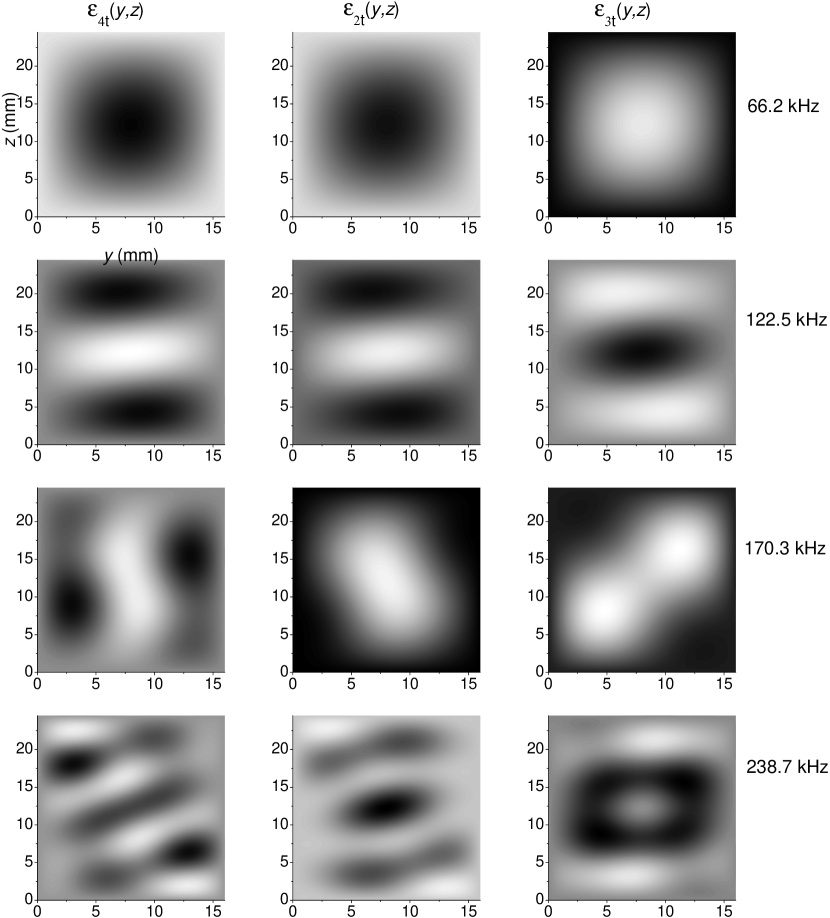
Figure 1: The distributions of the fluctuational parts of the strains $\varepsilon_{it}(y,z)/E_{1t}$ at different frequencies of a X-cut of Rochelle salt with $L_{y}=1.60$ cm, $L_{z}=2.45$ cm at 293 K.

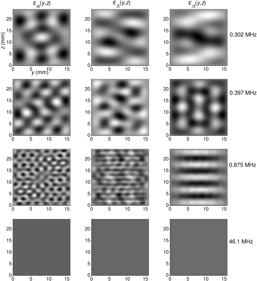
Figure 2: The same.

Figure 3 shows the frequency dependence of dynamic permittivity of the Rochelle salt X-cut (with $L_{y}=1.60$ cm, $L_{z}=2.45$ cm) within the entire frequency range of the current model applicability. That range does not include the region of the domain-related dispersion below 1 kHz [3, 1] or the submillimeter (100-700 GHz) region of resonant dispersion [8]. The experimental data shown by open symbols are for the frequencies outside the piezoelectric resonance regions of the samples used in the measurements, so the dimensions of those samples are irrelevant. The obtained evolution of the permittivity is analogous to the experimental [3] and to the previously obtained theoretical [13, 15] ones: from the static permittivity of a free crystal at low frequencies, via the piezoelectric resonance region ($10^{4}\div 10^{7}$ Hz for this sample dimensions), to the clamped crystal value, and, eventually, to a relaxational dispersion in the microwave region. A fairly good agreement with experiment is obtained.

Figure 3: Frequency dependence of dielectric permittivity of a X-cut of Rochelle salt at 293 K. Symbols are experimental points taken from [4] – $\blacksquare$, [7] – $\bigtriangledown$, [21] – $\circ$. The line: a theory. The line and $\blacksquare$ are for $L_{y}=1.60$ cm, $L_{z}=2.45$ cm. Other symbols correspond to samples of different sizes.

Now we take a closer look at the resonance region. Ability of the simplified system (27) to describe the resonant behavior of lattice strains and, henceforth, the dynamic dielectric permittivity of Rochelle salt X-cuts is demonstrated in fig. 4, showing the frequency dependence of the permittivity in the lower part of the resonant region. One can see that most of the resonant frequencies of the permittivity, calculated numerically, using the complete set of equations (17), are very well reproduced by the resonant frequencies of the simplified system (27).

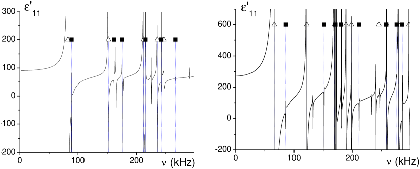
Figure 4: Frequency dependence of the dynamic dielectric permittivity of a Rochelle salt X-cut at 275 K (left) and 293 K (right). The solid line is calculated with $\overline{\varepsilon_{it}}$ found from (17). $\triangle$ and $\blacksquare$ are the resonant frequencies $\nu_{kl}^{(4)}$ and $\nu_{kl}^{(23)}$ of the simplified system (27). $L_{y}=1.60$ cm, $L_{z}=2.45$ cm.

The temperature dependence of a few lowest resonance frequencies of the simplified system (27) for this particular X-cut is shown in figure 5. It is seen that at all temperatures the lowest is the resonance frequency $\nu_{kl}^{(4)}=\omega_{kl}^{(4)}/2\pi$ associated with the shear mode at $k=l=0$. The lowest frequency $\nu_{kl}^{(23)}=\omega_{kl}^{(23)}/2\pi$ of the extensional modes (at $k=l=0$), active in the ferroelectric phase only, is higher at any temperature and at any sample dimensions and always remains finite. The shear mode frequencies $\nu_{kl}^{(4)}$, on the other hand, go to zero at the Curie temperatures at all $k$ and $l$.

The agreement with experiment for the lowest resonant frequency is quite good in the ferroelectric phase and gets worse in the upper paraelectric phase. It is, apparently, caused by a similar misfit for the elastic constant $c_{44}^{E}$ (see Eq. (24) and [19]).

       

Figure 5: Temperature dependence of the lowest resonance frequencies of the Rochelle salt X-cut with $L_{y}=1.60$ cm, $L_{z}=2.45$ cm. Lines: the theory. Solid lines: $\nu_{kl}^{(4)}$; dashed lines: $\nu_{kl}^{(23)}$. Symbols: experimental points of [4]. The numbers in parentheses are the $(k,l)$ values.

This disagreement is well revealed in the temperature variation of the dynamic dielectric permittivity of the Rochelle salt X-cut at 60 kHz shown in fig. 6 (left). There are two distinct and well resolved resonance peaks below and above the Curie point. With increasing frequency, these peaks move away from the Curie point. They are associated with the $\varepsilon_{4}$ shear mode and given by $\nu_{00}^{(4)}$. In the upper paraelectric phase, the disagreement between theory and experiment for $\nu_{res}$ seen in fig. 5 resulted in a more than 2 K difference between the theoretical and experimental temperatures of the resonant peak.

What has not been observed experimentally [4] is that apart from the two discussed peaks, in the close vicinity of the transition temperature, the permittivity also has a multitude of other resonances, which are higher order resonances of the $\varepsilon_{4}$ mode ($\nu_{kl}^{(4)}$ at $k+l>0$).

Actually, it follows from fig. 5 that at frequencies below the lowest resonant frequency of the extensional mode $\nu^{(23)}_{00}(T_{\rm C})$ at the Curie points (the threshold frequency which can be found from (36) at $c_{44}^{E}\to 0$; it equals 80 kHz for this particular X-cut), all resonances are associated with the shear $\varepsilon_{4}$ mode. Above $\nu^{(23)}_{00}(T_{\rm C})$, the resonances associated with the extensional modes appear in the ferroelectric phase.

The temperature curve of the permittivity in a wider temperature range shows (fig. 6, right) that the resonances form two packs around each Curie temperature, with the density of resonances increasing at approaching the Curie points. It can be shown that the pack widths increase with increasing frequency, which is caused by the shape of the $\nu_{kl+}^{(4)}(T)$ curves (see fig. 5) and by appearance of the $\nu_{kl}^{(23)}$ resonances. Eventually, at some sufficiently high frequency the packs overlap.

    

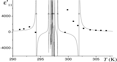
Figure 6: Temperature dependences of dynamic dielectric permittivity of the Rochelle salt X-cut with $L_{y}=1.60$ cm, $L_{z}=2.45$ cm at 60 kHz (left) and 800 kHz (right). Solid line: the theory. $\bullet$: experimental points of [4]; $\triangle$ are the resonant frequencies of the simplified system (27) given by (24).

5 Concluding remarks

Vibrations of X-cuts of Rochelle salt crystals and their influence on the dynamic dielectric permittivity are analyzed using the modified Mitsui model that takes into account the shear strain $\varepsilon_{4}$ and the diagonal strains $\varepsilon_{1}$, $\varepsilon_{2}$, $\varepsilon_{3}$ [16]. The system dynamics is described within the frequency range, starting from 1 kHz (above the dispersion associated with the domain wall motion) via the piezoelectric resonance region and the microwave relaxational dispersion up to about $10^{11}$ Hz.

Special attention is paid to the piezoelectric resonance region. Explicit expressions for the resonant frequencies, associated with the shear mode of $\varepsilon_{4}$ and with the extensional in-plane modes of $\varepsilon_{2}$, $\varepsilon_{3}$, of such cuts are derived. They are obtained at neglecting the out-of-plane mode associated with $\varepsilon_{1}$, as well as the elastic constants $c^{E}_{24}$ and $c^{E}_{34}$. The temperature behavior of the resonant frequencies is analyzed; it is shown that the lowest resonance is associated with the shear mode at all temperatures.

The changes in the calculated spatial distributions of the strains with increasing frequency visualize the effect of crystal clamping by the high-frequency electric field. Both the shear mode and the extensional modes are suppressed.

It is shown that the resonances associated with the extensional modes appear above a certain threshold frequency, and in the ferroelectric phase only, which is consistent with the symmetry considerations. In the close vicinities of the transition temperatures, the permittivity has a multitude of overlapping peaks, which are higher order resonances of the $\varepsilon_{4}$ mode.

References

• [1] J.F. Araujo, J. Mendes Filho et al, Phys. Rev. B 57, 783 (1998).
• [2] A.V. Shylโ€™nikov, N.M. Galijarova et al. Kristallografiya 31, 326 (1986).
• [3] Y.M.Poplavko, V.V.Meriakri, P.Pereverzeva, V.V.Alesheckin, and V.I.Molchanov, Fiz. Tverd. Tela (Leningrad) 15, 2515 (1974) [Sov. Phys. Solid State 15, 1672 (1974).
• [4] M.R.ย Leonovici and I.ย Bunget, Ferroelectrics 22, 835 (1979).
• [5] W.P.Mason, Phys. Rev. 55, 775 (1939).
• [6] H.ย Mueller, Phys. Rev. 58, 565 (1940).
• [7] F.ย Sandy and R.V.ย Jones, Phys. Rev. 168, 481 (1968).
• [8] A.A. Volkov, G.V. Kozlov, S.P. Lebedev, JETP 52, 722 (1980).
• [9] T. Mitsui, Phys. Rev. 111, 1259 (1958).
• [10] B. Zeks, G.C. Shukla, R.Blinc, Phys. Rev. B. 3, 2306 (1971).
• [11] B.Zeks, G.C.Shukla, R.Blinc, J. Phys. 33, supplement to N 4, c2-67-c2-68 (1972).
• [12] R.R.ย Levitskii, I.R.Zachek, T.M.Verkholyak, A.P.Moina, Condens. Matter Phys. 6, 261 (2003).
• [13] A.P.ย Moina, R.R.Levitskii and I.R.Zachek, Phys. Rev.ย B 71, 134108 (2005).
• [14] R.R.ย Levitskii, I.R.ย Zachek, T.M.ย Verkholyak, and A.P.ย Moina, Phys. Rev.ย B 67, 174112 (2003).
• [15] A. Andrusyk (2011). Piezoelectric Effect in Rochelle Salt, Ferroelectrics - Physical Effects, Mickael Lallart (Ed.), InTech, http://www.intechopen.com/articles/show/title/piezoelectric-effect-in-rochelle-salt
• [16] A.P.ย Moina, R.R.Levitskii and I.R.Zachek, Condens. Matter Phys. 14, 43602 (2011).
• [17] R.J. Glauber, J. Math. Phys. 4, 294 (1963).
• [18] W.P.ย Mason, Piezoelectric Crystals and Their Application to Ultrasonics (Van Nostrand, New York, 1950).
• [19] A.P.Moina, Condens. Matter Phys. 15 (2012). (to be published)
• [20] http://www.freefem.org/ff++
• [21] U. Schneider, P. Lunkenheimer, J. Hemberger, and A. Loidl, Ferroelectrics, 242, 71 (2000).