Theory of orbital magnetization in disordered systems

Abstract

We present a general formula of the orbital magnetization of disordered systems based on the Keldysh Green’s function theory in the gauge-covariant Wigner space. In our approach, the gauge invariance of physical quantities is ensured from the very beginning, and the vertex corrections are easily included. Our formula applies not only for insulators but also for metallic systems where the quasiparicle behavior is usually strongly modified by the disorder scattering. In the absence of disorders, our formula recovers the previous results obtained from the semiclassical theory and the perturbation theory. As an application, we calculate the orbital magnetization of a weakly disordered two-dimensional electron gas with Rashba spin-orbit coupling. We find that for the short range disorder scattering, its major effect is to the shifting of the distribution of orbital magnetization corresponding to the quasiparticle energy renormalization.

I Introduction

Magnetization is one of the most important and intriguing material properties. An adequate account of magnetization should not only include the contribution from the spin polarization of electrons, but also the contribution from the orbital motion of electrons. In crystals, due to the reduced spatial symmetry, the orbital contribution to the magnetization is usually quenched. However, in certain materials with topologically nontrivial band structures, large contributions can arise from the effective reciprocal space monopoles near the band anti-crossings. Several different methods have been employed to study the orbital magnetization (OM) in crystals Hirst ; Xiaod ; Thonhauser11 ; Xiao ; Yao ; Thonhauser ; Ceresoli06 ; Souza ; Shi ; Ceresoli07 ; Ceresoli ; Resta ; Restab ; Gata ; Gatb ; wanga ; wangb . One major difficulty in the calculation is posed by the evaluation of the operator Hirst ; Xiaod $\hat{\bm{r}}\times\hat{\bm{j}}$, because the the position $\hat{\bm{r}}$ is ill-defined in the Bloch representation. This difficulty can be avoided in a semiclassical picture or be circumvented by a transformation to the Wannier representation. Xiao et al. Xiao ; Yao presented a general formula for OM for metal and insulator, derived from a semiclassical formalism with the Berry phase corrections. Thonhauser et al. Thonhauser ; Ceresoli06 derived an expression of the OM for periodic insulators using the Wannier representation. From the elementary thermodynamics, Shi et al. Shi obtained a formula for the OM in a periodic system using the standard perturbation theory. Their result can in principle take into account the electron-electron interaction effects. A computation of the OM for periodic systems with density-functional theory was carried out by Ceresoli et al. Ceresoli .

Previous studies are mainly concerned with clean systems. However, real crystals are never perfect, disorders such as defects, impurities, phonons etc. constantly break the translational symmetry and lead to scattering events. The effect of disorder scattering on the OM has not been carefully studied so far. On one hand, the OM is a thermodynamic quantities, hence it is expected to be less susceptible to disorder scattering. On the other hand, the appearance of current operator $\hat{\bm{j}}$ in the definition suggests behaviors similar to transport quantities which might be strongly affected by the disorder scattering. Therefore, it is important and desirable to have a good understanding of the role played by the disorder scattering in the OM.

In this paper, we present a general formula of the OM in disordered systems based on the Keldysh Green’s function theory in the gauge-covariant Wigner space Onoda06 ; Onoda ; Onoda08 ; Sinova ; Haug . This approach was developed as a systematic approach to the nonequilibrium electron dynamics under external fields. Our formula derived from this approach shares the advantage of being able to capture the disorder effects in a systematic way and ensure the gauge invariance property from the very beginning. We show that in the clean limit, our formula reduces to the previous results obtained from other approaches. As an application, we study the OM in a disordered two-dimensional electron gas with the Rashba spin-orbit coupling. We find that the OM is robust against short range disorders. The main effect of the scattering by short range disorders is a rigid shift of the distribution of OM in energy.

The structure of this paper is organized as follows. In Sec. II.1, we outline the Keldysh Green’s function formalism which is employed for our derivation. Our general formula of OM is presented in Sec. II.2. In Sec. III, we apply the formula to study the OM of a two-dimensional disordered electron gas with the Rashba spin-orbit coupling. Summary and conclusion are given in Sec. IV. Some details of the calculation are provided in the appendices.

II Orbital magnetization of disordered systems

II.1 Keldysh Green’s function formalism

We employ the Keldysh Green’s function formalism in the Wigner representation Onoda06 , which has recently been used to study the current response of multi-band systems under an electric field Onoda ; Onoda08 . In the Wigner representation, Green’s functions and the self-energies are expressed as functions of the center-of-mass coordinates ($T$,$\bm{X}$), the energy $\varepsilon$ and the mehanic momentum p. The energy and the mechanic momentum are the Fourier transforms of the relative time and space coordinates respectively.

The Dyson equations in the presence of external electromagnetic fields can be written as

$$\left[\varepsilon\underline{\hat{I}}-\underline{\hat{H}}_{0}(\textbf{p})-\underline{\hat{\Sigma}}(\varepsilon)\right]\star\underline{\hat{G}}(\varepsilon,\textbf{p}) = \underline{\hat{I}},$$ (1a)

$$\underline{\hat{G}}(\varepsilon,\textbf{p})\star\left[\varepsilon\underline{\hat{I}}-\underline{\hat{H}}_{0}(\textbf{p})-\underline{\hat{\Sigma}}(\varepsilon)\right] = \underline{\hat{I}}.$$ (1b)

Each quantity with an underline in the above equations is a matrix in Keldysh space. Specifically, we have

$$\begin{matrix}\underline{\hat{G}}&\equiv&\left(\begin{array}[]{cc}\hat{G}^{R}&2\hat{G}^{<}\\ 0&\hat{G}^{A}\end{array}\right),\end{matrix}\quad\begin{matrix}\underline{\hat{\Sigma}}&\equiv&\left(\begin{array}[]{cc}\hat{\Sigma}^{R}&2\hat{\Sigma}^{<}\\ 0&\hat{\Sigma}^{A}\end{array}\right),\end{matrix}$$ (2)

$$\begin{matrix}\underline{\hat{H}}_{0}&\equiv&\left(\begin{array}[]{cc}\hat{H}_{0}&0\\ 0&\hat{H}_{0}\end{array}\right),\end{matrix}\quad\begin{matrix}\underline{\hat{I}}&=&\left(\begin{array}[]{cc}\hat{\sigma}^{0}&0\\ 0&\hat{\sigma}^{0}\end{array}\right),\end{matrix}$$ (3)

where $\hat{G}^{(R,A,<)}$ are the (retarded, advanced, lesser) Green functions, and $\hat{\Sigma}^{(R,A,<)}$ are the corresponding self-energies, $\hat{H}_{0}$ is the Hamiltonian in the absence of external electromagnetic fields, $\hat{\sigma}^{0}$ is the identity matrix. The $\star$ operator in Eq.(1) is defined as

$$\star\equiv\exp\left[\frac{iq\hbar}{2}F^{\mu\nu}\left(\overleftarrow{\partial}_{p^{\mu}}\overrightarrow{\partial}_{p^{\nu}}-\overleftarrow{\partial}_{p^{\nu}}\overrightarrow{\partial}_{p^{\mu}}\right)\right],$$ (4)

with the differential operators $\overleftarrow{\partial}$ and $\overrightarrow{\partial}$ operating on the left-hand and the right-hand sides respectively, $\bm{q}=-\left|e\right|$ is the electron charge, and $F^{\mu\nu}=\partial_{X_{\mu}}A^{\nu}(X)-\partial_{X_{\nu}}A^{\mu}(X)$ is the electromagnetic field tensor, $\mu$ and $\nu$ label the four dimensional space-time components and the Einstein summation convention is assumed. It should be noted that the energy $\varepsilon$ and the mechanic momentum p include the electromagnetic potentials $A^{\mu}(X)$, both are gauge invariant quantities. The $\star$ operator in Eq.(1) only involves the physical fields, so it is also gauge invariant. In this formalism the gauge invariance is respected from the very beginning and easily maintained during the perturbative expansion, which is an important advantage Onoda06 .

Here we consider the situation with a uniform weak magnetic field along the z-direction, i.e. $\textbf{B}=(0,0,B)$. Then the various quantities can be expanded in terms of $B$. In particular, Green’s functions and the self-energies can be expressed as

$$\hat{G}^{\alpha}(\varepsilon,\textbf{p}) = \hat{G}^{\alpha}_{0}(\varepsilon,\textbf{p})+e\hbar B\hat{G}^{\alpha}_{B}(\varepsilon,\textbf{p})+O(B^{2}),$$ (5)

$$\hat{\Sigma}^{\alpha}(\varepsilon) = \hat{\Sigma}^{\alpha}_{0}(\varepsilon)+e\hbar B\hat{\Sigma}^{\alpha}_{B}(\varepsilon)+O(B^{2}),$$ (6)

with $\alpha=R,A,<$ for the retarded, advanced and lesser components respectively. Here functions with the subscript 0 are of zeroth order in the external magnetic field strength (note that they include scattering effects). We have

$$\hat{G}^{R(A)}_{0}(\varepsilon,\textbf{p})=\left[\varepsilon-\hat{H}_{0}(\textbf{p})-\hat{\Sigma}^{R(A)}_{0}(\varepsilon)\right]^{-1},$$ (7)

$$\hat{G}^{<}_{0}(\varepsilon,\textbf{p})=\left[\hat{G}^{A}_{0}(\varepsilon,\textbf{p})-\hat{G}^{R}_{0}(\varepsilon,\textbf{p})\right]f(\varepsilon),$$ (8)

where $f(\varepsilon)$ is the Fermi distribution. The functions with subscript $B$ are the linear response coefficient to the external field. They can be solved from the Dyson equation. It is usually convenient to decompose the lesser component $\hat{G}^{<}_{B}$ and $\hat{\Sigma}^{<}_{B}$ (which are related to particle distribution) into two parts, with one part from the Fermi surface and the other part from the Fermi sea Streda ,

$$\hat{G}^{<}_{B}(\varepsilon,\textbf{p})\!\!=\hat{G}^{<}_{B,I}(\varepsilon,\textbf{p})\partial_{\varepsilon}f(\varepsilon)\!\!+\!\!\hat{G}^{<}_{B,II}(\varepsilon,\textbf{p})f(\varepsilon)$$ (9)

$$\hat{\Sigma}^{<}_{B}(\varepsilon)=\hat{\Sigma}^{<}_{B,I}(\varepsilon)\partial_{\varepsilon}f(\varepsilon)+\hat{\Sigma}^{<}_{B,II}(\varepsilon)f(\varepsilon).$$ (10)

From the Dyson equation (kept to the linear order in $B$), it is straightforward to show that

$$\hat{G}^{<}_{B,I}=\hat{\Sigma}^{<}_{B,I}=0,\\$$ (11)

i.e. there is no Fermi surface term in the linear order lesser component, and for the Fermi sea term we have

$$\hat{G}^{<}_{B,II}(\varepsilon,\textbf{p})=\hat{G}^{A}_{B}(\varepsilon,\textbf{p})-\hat{G}^{R}_{B}(\varepsilon,\textbf{p}),$$ (12)

$$\hat{\Sigma}^{<}_{B,II}(\varepsilon)=\hat{\Sigma}^{A}_{B}(\varepsilon)-\hat{\Sigma}^{R}_{B}(\varepsilon).$$ (13)

The retarded and advanced Green’s function $\hat{G}^{R(A)}_{B}$ and self-energy $\hat{\Sigma}^{R(A)}_{B}$ are determined from the following self-consistent equations

$$\hat{G}^{R(A)}_{B} = \frac{i}{2}\left[\hat{G}^{R(A)}_{0}\hat{v}_{x}(\partial_{p_{y}}\hat{G}^{R(A)}_{0})-(\partial_{p_{y}}\hat{G}^{R(A)}_{0})\hat{v}_{x}\hat{G}^{R(A)}_{0}\right]$$ (14)

$$+\hat{G}^{R(A)}_{0}\hat{\Sigma}^{R(A)}_{B}\hat{G}^{R(A)}_{0},$$

where the velocity operator is defined as $\hat{v}_{i}\equiv\frac{1}{i\hbar}\left[\hat{x}_{i},\hat{H}\right]$.

In this approach, the disorder effects are captured by the self-energies $\hat{\Sigma}^{R(A)}_{0}$ and $\hat{\Sigma}^{R(A)}_{B}$, which allows a systematic perturbative treatment. In the weak disorder regime, the self-consistent $T$-matrix approximation provides a good approximation scheme. In this approximation, we have

$$\hat{\Sigma}^{R(A)}_{0}(\varepsilon) = n_{\rm{imp}}\hat{T}^{R(A)}_{0}(\varepsilon),$$ (15)

and

$$\hat{\Sigma}^{R(A)}_{B}(\varepsilon)\! = \!n_{\rm imp}\hat{T}^{R(A)}_{0}(\varepsilon)\!\!\int\!\!\!\frac{d^{2}\textbf{p}}{(2\pi\hbar)^{2}}\!\hat{G}^{R(A)}_{B}(\varepsilon,\textbf{p})\hat{T}^{R(A)}_{0}(\varepsilon)\!,$$

where $n_{\rm imp}$ is the impurity concentration and the $T$-matrix is expressed as

$$\hat{T}^{R(A)}_{0}(\varepsilon) = \hat{V}_{\text{imp}}\left(1-\int\frac{d^{2}\textbf{p}}{(2\pi\hbar)^{2}}\hat{G}^{R(A)}_{0}(\varepsilon,\textbf{p})\hat{V}_{\text{imp}}\right)^{-1},$$

with $\hat{V}_{\text{imp}}$ being the impurity potential.

The equilibrium Green’s functions $\hat{G}^{R(A)}_{0}$ and the self energies $\hat{\Sigma}^{R(A)}_{0}$ can be obtained by solving Eqs. (7),  (15) and  (LABEL:eq:g^R,A:0) self-consistently. Then the linear order coefficients $\hat{G}^{R(A)}_{B}$ and $\hat{\Sigma}^{R(A)}_{B}$ can be solved from Eqs. (14) and  (LABEL:eq:Sigma^R,A:b). Finally, we can obtain $\hat{G}^{<}_{B,II}$ through Eq. (12) and the linear response of the system in the external magnetic field can be completely determined.

The lesser Green’s function contains the information of particle distribution. In our case, both the external magnetic field and the disorder scattering affect the quasiparticle distribution. Before we proceed, it is interesting to observe how the non-trivial band geometry (described by the Berry curvature) can be captured by the present Wigner space Green’s function formalism. For a homogeneous system, the electron density can be written as

$$\bm{n}_{e}=\frac{1}{i}\int\frac{d\varepsilon}{2\pi}\int\frac{d^{2}\textbf{p}}{(2\pi\hbar)^{2}}\mathrm{tr}\left[\hat{G}^{<}(\varepsilon,\textbf{p})\right].$$ (18)

In the absence of the disorder scattering, the eigenstates are well-defined Bloch states grouped into energy bands. Using the theorem of residues, we can express the ground state electron density in the presence of a constant magnetic field as (see Appendix C)

$$\bm{n}_{e} = \sum_{n,occ}\int\!\frac{d^{2}\textbf{p}}{(2\pi\hbar)^{2}}\left[1+\frac{e}{\hbar}\textbf{B}\cdot\bm{\Omega}_{n}(\textbf{p})\right].$$ (19)

The summation is over all the occupied states, and $\bm{\Omega}_{n}(\textbf{p})\!=\!i\langle{\bm{\nabla}_{\textbf{p}}u_{n\textbf{p}}|\times|\bm{\nabla}_{\textbf{p}}u_{n\textbf{p}}}\rangle$ is the Berry curvature of the Bloch state $|n,\textbf{p}\rangle=e^{i\textbf{p}\cdot\textbf{x}/\hbar}|u_{n\textbf{p}}\rangle$. It can be seen that the Fermi-sea volume is changed linearly by a magnetic field when the Berry curvature is nonzero. This effect was previous interpreted as the modification of phase space density of states Xiao .

II.2 Formula of orbital magnetization

We start from the standard thermodynamic definition of the OM density at zero temperature Shi :

$$\bm{M}=-\left(\frac{\partial K}{\partial\bm{B}}\right)_{\mu},$$ (20)

where $K=E-\mu N$ is the grand thermodynamic potential, $B$ is a weak magnetic field. Since we are concerned with the orbital contribution, the small Zeeman coupling between the electron spin and external field will be dropped. The potential $\bm{K}$ can be expressed through the lesser Green’s function,

$$\bm{K}=\frac{1}{i}\int\frac{d\varepsilon}{2\pi}\int\frac{d^{2}\textbf{p}}{(2\pi\hbar)^{2}}\mathrm{tr}\left[\left(\hat{H}-\mu\right)\hat{G}^{<}(\varepsilon,\textbf{p})\right].$$ (21)

Using Eqs. (20),  (21) and  (9), we find that the OM can be written as

$$\bm{M} = -ie\hbar\int\frac{d\varepsilon}{2\pi}\int\frac{d^{2}\textbf{p}}{(2\pi\hbar)^{2}}\mathrm{tr}\left[\left(\hat{H}-\mu\right)\right.$$ (22)

$$\times\left.\left(\hat{G}^{A}_{B}(\varepsilon,\textbf{p})-\hat{G}^{R}_{B}(\varepsilon,\textbf{p})\right)\right]f(\varepsilon).$$

From this expression, we can see that the OM has contributions from the whole Fermi sea, with no separate Fermi surface contribution such as that for the transport quantities.

In this formula, the impurity scattering effect comes in through two terms: the self-energy $\hat{\Sigma}^{R,A}_{0}$ which modifies the ground state electronic structure and the vertex corrections associated with $\hat{\Sigma}^{R,A,<}_{B}$ which represent an interplay between the magnetic field and the impurity scattering. We may separate out the terms containing $\hat{\Sigma}^{R,A,<}_{B}$ and write the OM explicitly as

$$\bm{M}=\bm{M}^{I}+\bm{M}^{II},$$ (23)

where

$$\bm{M}^{I}=\frac{e\hbar}{2} \int\!\frac{d\varepsilon}{2\pi}f(\varepsilon)\int\!\frac{d^{2}\textbf{p}}{(2\pi\hbar)^{2}}$$

$$\times\sum_{ij}\text{Tr} \left[\epsilon_{ij}(\hat{H}-\mu)\hat{G}^{A}_{0}(\varepsilon,\textbf{p})\hat{v}_{i}\hat{G}^{A}_{0}(\varepsilon,\textbf{p})\hat{v}_{j}\hat{G}^{A}_{0}(\varepsilon,\textbf{p})\right.$$ (24)

$$\left.-(\hat{G}^{A}_{0}\rightarrow\hat{G}^{R}_{0})\right],$$

and

$$\bm{M}^{II}=-ie\hbar\int\!\frac{d\varepsilon}{2\pi}f(\varepsilon)\int\!\frac{d^{2}\textbf{p}}{(2\pi\hbar)^{2}}$$

$$\times\text{Tr}\left[(\hat{H}-\mu)\hat{G}^{A}_{0}\hat{\Sigma}^{A}_{B}\hat{G}^{A}_{0}-(\hat{H}-\mu)\hat{G}^{R}_{0}\hat{\Sigma}^{R}_{B}\hat{G}^{R}_{0}\right],$$ (25)

where $\epsilon_{ij}$ with $i,j\in\{x,y\}$ is the 2D antisymmetric tensor, and the second term in the bracket in Eq.(24) means that the second term is the same as the first term except that all the $\hat{G}^{A}_{0}$ are replaced by $\hat{G}^{R}_{0}$. Such a decomposition scheme was also adopted in the study of anomalous Hall conductivity Onoda08 , and in that context, the two parts are referred to as the intrinsic part and extrinsic part respectively. It should be noted that the intrinsic part $\bm{M}^{I}$ also has impurity scattering effects in it (see Eq. (7) and Eq. (15)), it is intrinsic in the sense that it only contains quantities that are of zeroth order in the external field. As for the extrinsic part $\bm{M}^{II}$, it is easy to see that it is already linear order in $n_{\rm imp}$ (see Eq. (LABEL:eq:Sigma^R,A:b)). Therefore in the weak scattering regime, the extrinsic part is expected to be much smaller than the intrinsic part.

The above formula is our main result. From this formula, we see that there is no separate Fermi surface contributions like those in the transport quantities, which is consistent with OM being a thermodynamic equilibrium property. This formula applies for both insulators and metals. The quantities in this formula can be calculated from the Dyson equation according to our prescription described in the previous section. It can also be straightforwardly implemented in the numerical calculation, either from effective models or from first principles.

In the clean limit, we only have the intrinsic part. The general result reduces to (see Appendix D for the derivation)

$$\bm{M} = \sum_{n\textbf{p}}f_{n\textbf{p}}\left[\bm{m}_{n}(\textbf{p})-\frac{e}{\hbar}(\epsilon_{n\textbf{p}}-\mu)\bm{\Omega}_{n}(\textbf{p})\right],$$ (26)

where $\bm{m}_{n}(\textbf{p})\!=\!(e/2\hbar)i\langle\bm{\nabla}_{\textbf{p}}u_{n\textbf{p}}|[\epsilon_{n}(\textbf{p})-\hat{H}_{0}(\textbf{p})]\times|\bm{\nabla}_{\textbf{p}}u_{n\textbf{p}}\rangle$ is the orbital moment of the Bloch state $|n,\textbf{p}\rangle$ and $\bm{\Omega}_{n}(\textbf{p})\!=\!i\langle{\bm{\nabla}_{\textbf{p}}u_{n\textbf{p}}|\times|\bm{\nabla}_{\textbf{p}}u_{n\textbf{p}}}\rangle$ is the Berry curvature. The first term in Eq. (26) is a sum of the orbital magnetic moments associated with each Bloch state Chang ; Sundaram , and the second term is a Berry-phase correction to the OM. Therefore, the OM can be written as

$$\bm{M} = \mathcal{M}_{\text{m}}+\mathcal{M}_{\Omega}.$$ (27)

This clean limit result was previously derived from the standard perturbation theory of quantum mechanics by Shi et al.  Shi and also from the semiclassical theory by Xiao et al.  Xiao . Now it is also reproduced as a special limiting case of our general formula.

III Application to a two-dimensional electron gas with Rashba spin-orbit coupling

III.1 Model

We apply our theory to study the model of a two-dimensional disordered electron gas with Rashba spin-orbit coupling. The Hamiltonian for the system reads

$$\hat{H} = \hat{H}_{0}+\hat{H}_{\text{imp}},$$ (28a)

$$\hat{H}_{0} = \frac{p^{2}}{2m}\hat{\sigma}^{0}+\alpha\left(p_{x}\hat{\sigma}^{y}-p_{y}\hat{\sigma}^{x}\right)-\Delta_{0}\hat{\sigma}^{z},$$ (28b)

$$\hat{H}_{\text{imp}} = u_{\text{imp}}\hat{\sigma}^{0}\sum_{\vec{r}_{\rm imp}}\delta(\vec{r}-\vec{r}_{\rm imp}),$$ (28c)

where $(\hat{\sigma}^{x},\hat{\sigma}^{y},\hat{\sigma}^{z})$ are the three Pauli matrices and $\hat{\sigma}^{0}$ is the identity matrix, $\alpha$ is the strength of the spin-orbit coupling, and term $-\Delta_{0}\hat{\sigma}^{z}$ is the spin splitting which can be introduced by the exchange coupling with a nearby ferromagnet or magnetic dopants. $\hat{H}_{\text{imp}}$ is the disorder potential from the randomly distributed short range impurities with strength $u_{\text{imp}}$. The energy dispersion of the Hamiltonian $\hat{H}_{0}$ is given by

$$\bm{E}_{\lambda}(p)=\frac{p^{2}}{2m}-(-1)^{\lambda}\sqrt{\Delta^{2}_{0}+\alpha^{2}p^{2}},$$ (29)

where $\lambda=1,2$ labels the upper and lower band respectively. When the Rashba coupling energy scale Garelli $m\alpha^{2}$ is larger than the Zeeman coupling strength the minima of the lower band occur at a finite wave vector and the dispersion assumes a Mexican hat shape (see Fig. 1 (a)). When the Zeeman coupling dominates over the Rashba energy, the minimum of the lower band $\bm{E}_{2}$ occurs at the origin (see Fig. 2 (a)).

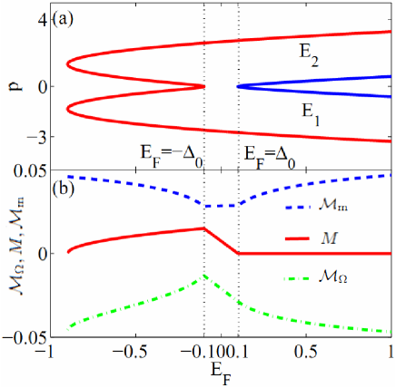
Figure 1: (Color online) (a) Electronic band dispersions of our model given by Eq. (29). (b) Orbital magnetization ($\bm{M}$, solid red curve) of disordered free system and its two components $\mathcal{M}_{\text{m}}$ (dashed blue curve) and $\mathcal{M}_{\Omega}$ (dash-dotted green curve) as functions of Fermi energy $E_{F}$. They are plotted in units of $e/{\hbar}$. The parameters are chosen as $2m\alpha^{2}=3.59$ and $\Delta_{0}=0.1$.

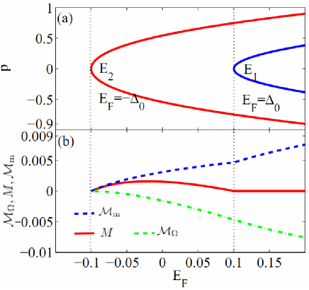
Figure 2: (Color online) (a) Electronic band dispersions of our model given by Eq. (29). (b) Orbital magnetization ($\mathcal{M}$, solid red curve) of disorder free system and its two components $\mathcal{M}_{\text{m}}$ (dashed blue curve) and $\mathcal{M}_{\Omega}$ (dash-dotted green curve) as functions of Fermi energy $E_{F}$. They are plotted in units of $e/{\hbar}$. The parameters are chosen as $2m\alpha^{2}=0.08$ and $\Delta_{0}=0.1$.

Let’s first consider the clean limit, in which case the orbital magnetic moment and the Berry curvature of each Bloch state can be calculated straightforwardly:

$$\bm{m}_{1}(\bm{p})=\bm{m}_{2}(\bm{p})=\frac{e}{2\hbar}\frac{\Delta_{0}\alpha^{2}}{\Delta^{2}_{0}+\alpha^{2}p^{2}},$$ (30)

$$\bm{\Omega}_{1}(\bm{p})=-\bm{\Omega}_{2}(\bm{p})=-\frac{1}{2}\frac{\Delta_{0}\alpha^{2}}{(\Delta^{2}_{0}+\alpha^{2}p^{2})^{\frac{3}{2}}}.$$ (31)

It is interesting to observe that for the same wavevector the orbital moments of the two bands have the same magnitude and the same sign, while the Berry curvatures have the same magnitude but opposite signs. It should also be noted that both the orbital moment and the Berry curvature would vanish if either $\alpha$ or $\Delta_{0}$ vanishes. From Eq.(26), we further see that the OM is nonzero only when both the spin-orbit coupling and the exchange coupling are present.

Analytical expressions of the OM can be easily obtained for the clean limit using Eq.(26). For example, for the case with $E_{F}>\Delta_{0}$, we have

$$\bm{M} = \frac{e\Delta_{0}}{4\pi\hbar}(E_{F}\!+\!\frac{\Delta^{2}_{0}}{2m\alpha^{2}})\left[\frac{1}{(\Delta^{2}_{0}+\alpha^{2}p_{F_{1}}^{2})^{\frac{1}{2}}}\!-\!\frac{1}{(\Delta^{2}_{0}+\alpha^{2}p_{F_{2}}^{2})^{\frac{1}{2}}}\right]$$ (32)

$$+\frac{e\Delta_{0}}{8\pi m\hbar\alpha^{2}}[(\Delta^{2}_{0}+\alpha^{2}p_{F_{1}}^{2})^{\frac{1}{2}}-(\Delta^{2}_{0}+\alpha^{2}p_{F_{2}}^{2})^{\frac{1}{2}}],$$

where $p_{F_{1,2}}$ is the Fermi momenta of the two bands.

III.2 Results

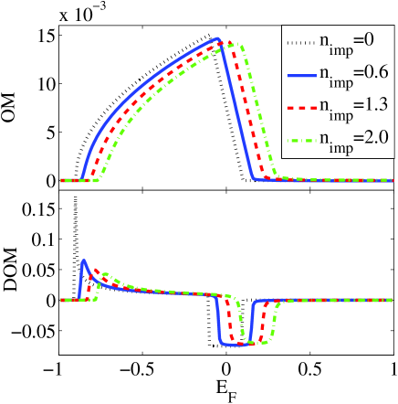
Figure 3: (Color online) (a) Orbital magnetization (OM) as a function of Fermi energy $E_{F}$ with different impurity concentration $n_{\text{imp}}$. (b) Density of OM with different impurity concentration $n_{\text{imp}}$. These quantities are plotted in units of $e/{\hbar}$. The parameters are chosen as $2m\alpha^{2}=3.59$, $\Delta_{0}=0.1$, and $u_{\text{imp}}=0.1$.

Now we analyze the OM of the disordered 2D Rashba model in detail. The calculation procedure follows our discussion in Sections  II.1 and  II.2. Since we have seen that both the spin-orbit coupling and the exchange coupling are essential ingredient for the OM, in the following we shall consider two different regimes of the model determined by the competition between the Rashba spin-orbit coupling and the exchange coupling. For each regime, we first analyze the clean limit where the physical picture is more transparent, and then study the influence of disorder scattering which is the focus in this paper.

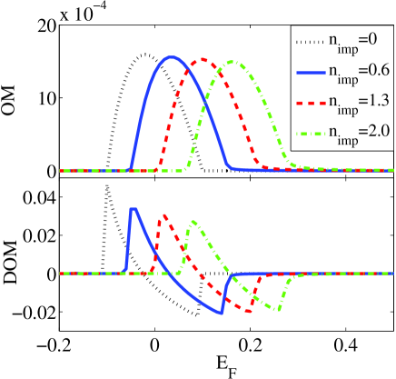
Figure 4: (Color online) (a) Orbital magnetization (OM) as a function of Fermi energy $E_{F}$ with different impurity concentration $n_{\text{imp}}$. (b) Density of OM with different impurity concentration $n_{\text{imp}}$. These quantities are plotted in units of $e/{\hbar}$. The parameters are chosen as $2m\alpha^{2}=0.08$, $\Delta_{0}=0.1$, and $u_{\text{imp}}=0.1$.

We first consider the regime where the Rashba coupling dominates over the exchange coupling, i.e. $2m\alpha^{2}\gg\Delta_{0}$. The typical band dispersion in this regime is shown in Fig. 1 (a) (with $2m\alpha^{2}=3.59$ and $\Delta_{0}=0.1$). In this regime, the bottom of the lower band occurs at a finite wavevector. The energy spectrum around the origin has an effective Dirac cone structure with a local gap $2\Delta_{0}$ at $p=0$. Both the orbital moment and the Berry curvature are concentrated near this band anticrossing point, as is evident from Eqs.(30) and (31). Fig. 1 (b) shows the OM for the clean limit. The orbital moment contribution $\mathcal{M}_{\text{m}}$ and the Berry curvature contribution $\mathcal{M}_{\Omega}$ are also plotted in Fig. 1 (b). We can see that as the Fermi energy $E_{F}$ increases from the lower band bottom, $\mathcal{M}_{\Omega}$ increases while $\mathcal{M}_{\text{m}}$ decreases. The increasing rate of $\mathcal{M}_{\Omega}$ is higher than the decreasing rate of $\mathcal{M}_{\text{m}}$, so the overall OM is increasing. The OM reaches its maximum when $E_{F}=-\Delta_{0}$, which corresponds to the local band top around the origin in momentum space. As the Fermi energy sweeps across the local energy gap between $-\Delta_{0}$ and $+\Delta_{0}$, the OM decreases approximately linearly with $E_{F}$. The linearity can be understood by noticing that from Eq.(26)) the derivative of the OM with respect to $E_{F}$ is just the momentum space integral of the Berry curvature. The Berry curvature distribution is concentrated near the band anticrossing point, corresponding to the small region around the origin in the present model. When the Fermi energy is within the gap, the Berry curvature integral only has contribution from the lower band and is almost constant, therefore leading to the linear energy dependence of OM. This linear decrease of OM stops when the Fermi energy touches the bottom of the upper band at $+\Delta_{0}$. Above the upper band bottom, $\mathcal{M}_{\Omega}$ and $\mathcal{M}_{\text{m}}$ almost cancel each other and the OM is vanishingly small. Throughout the spectrum, $\mathcal{M}_{\text{m}}$ is positive while $\mathcal{M}_{\Omega}$ is negative, corresponding to the paramagnetic and diamagnetic responses respectively. This has a clear explanation in the semiclassical picture: $\mathcal{M}_{\text{m}}$ is due to the self-rotation of the wavepacket which is paramagnetic, while $\mathcal{M}_{\Omega}$ is from the center-of-mass motion of the wavepacket hence is diamagnetic Xiaod .

When the exchange coupling dominates over the Rashba energy, The minimum of the lower band occurs at the origin. Compared with the previous case, there is no local gap at $p=0$. The typical band dispersion is shown in Fig. 2 (a) (with $\Delta_{0}=0.1$ and take $2m\alpha^{2}=0.08$). The overall shape of the OM is similar to that for the first case. Its distribution over spectrum is mainly below the upper band bottom. However, due to the absence of the local gap, the kink point at $-\Delta_{0}$ in Fig. 1 (a) merges with the lower band bottom. Moreover, the two contributions $\mathcal{M}_{\Omega}$ and $\mathcal{M}_{\text{m}}$ strongly cancel each other and the resulting OM is much smaller.

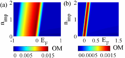
Figure 5: (Color online) Orbital magnetization (OM) as functions of Fermi energy $E_{F}$ and the impurity concentration $n_{\text{imp}}$ in units of $e/{\hbar}$. The parameters are chosen as $\Delta_{0}=0.1$, and $u_{\text{imp}}=0.1$, except the Rashba energy: (a) $2m\alpha^{2}=3.59$, (b) $2m\alpha^{2}=0.08$.

Now let’s consider the effects of disorder scattering on the OM in our model. When the disorder scattering is turned on, the translational invariance is broken. We can no longer define quantities such as $\mathcal{M}_{\Omega}$ and $\mathcal{M}_{\text{m}}$. Their effects are merged into the sophisticated expression in Eq.(23). Fig. 3 (a) and Fig. 4 (a) show the OM versus $E_{F}$ for the two regimes we discussed above. The different curves in each figure correspond to different impurity concentrations $n_{\text{imp}}$. Compared with the clean limit where $n_{\text{imp}}=0$, we see that the shape of the OM curve is almost unchanged but mainly its position is shifted by the scattering. This behavior is more obvious when we look at the density of OM shown in Fig. 3 (b) and Fig. 4 (b). For the clean limit, we see that the major contribution to the OM is from the states at the band bottom and at the local band edge. The effect of disorder scattering here is to shift the the density of OM distribution in energy. Such a shift can be understood by noticing that the OM only has the Fermi sea contribution. The main effect of scattering in Eq.(23) is the shift of energy arising from the real part of the self-energy correction Groth . For the short range disorder model, the disorder potential is a constant in momentum space, hence the self-energy is independent of the state, which results in a rigid energy shift for all the states. For a general disorder potential, the energy shift would be generally different for different states therefore the distribution of OM would be distorted. The effects of finite range disorders are currently under investigation.

To leading order, the shift should be linear in the disorder density $n_{\text{imp}}$. In Fig. 5 we plot the OM as a function of $E_{F}$ and $n_{\text{imp}}$. The linear dependence of the energy shift in $n_{\text{imp}}$ is clearly observed. Apart from the energy shift, the scattering induced state broadening is manifested as the smoothing of the peaks of the density of OM, which can be clearly observed in Fig. 3 (b) and Fig. 4 (b). The peaks of OM are only slightly decreased by the scattering. This means that the OM carried by the electronic states are quite robust against scattering.

IV Conclusions

In summary, we have derived a formula of the the OM of disordered electron systems based on the Keldysh Green’s function theory. This approach was developed as a systematic approach to the nonequilibrium electron dynamics under external fields. In the formula, OM is expressed in terms of the Green’s functions and self-energies, which can be solved from the Dyson equations, and systematic approximation schemes to the disorder effects can be employed. We find that there is no Fermi surface contribution like in the case of the current response. Our formula applies not only for insulators but also for metallic systems, where the quasiparicle behavior is usually strongly modified by the disorder scattering. It can also be straightforwardly implemented in the numerical calculation. In the clean limit, our formula reduces to the previous result obtained from other approaches. As an application, we calculate the OM of a weakly disordered two dimensional electron gas with Rashba spin-orbit coupling. The result shows that in the simplest white noise short range disorder model, the OM is robust against weak scattering and the main effect of scattering is a rigid shift of the distribution of OM in energy, which can be attributed to the real part of the self energy.

Appendix A Self-consistent equation for $\hat{\Sigma}^{R}_{0}$ and explicit forms of $\hat{G}^{R}_{0}$

The Green functions and self-energies in the absence of the external fields are obtained from the coupled self-consistent equations (7),  (15) and  (LABEL:eq:g^R,A:0). In our model, a direct analytical integration in $\varepsilon$ shows that

$$\Sigma^{R0}_{0}(\varepsilon) = \frac{n_{\rm imp}u_{\text{imp}}\left(1-u_{\text{imp}}g^{R0}_{0}(\varepsilon)\right)}{(1-u_{\text{imp}}g^{R0}_{0}(\varepsilon))^{2}-u_{\text{imp}}^{2}g^{Rz}_{0}(\varepsilon)^{2}},$$ (33)

$$\Sigma^{Rz}_{0}(\varepsilon) = \frac{n_{\rm imp}u_{\text{imp}}^{2}g^{Rz}_{0}(\varepsilon)}{(1-u_{\text{imp}}g^{R0}_{0}(\varepsilon))^{2}-u_{\text{imp}}^{2}g^{Rz}_{0}(\varepsilon)^{2}},$$ (34)

$$\Sigma^{Rx}_{0}(\varepsilon) = \Sigma^{Ry}_{0}(\varepsilon)=0,$$ (35)

$$g^{R0}_{0}(\varepsilon) = \frac{m}{4\pi\hbar^{2}}\sum_{\sigma}\ln\frac{G^{R}_{0}(\varepsilon,\Lambda,\sigma)}{G^{R}_{0}(\varepsilon,0,\sigma)}-m\alpha^{2}\tilde{g}^{R}_{0}(\varepsilon),\ \ \ \ \ \ \ \$$ (36)

$$g^{Rz}_{0}(\varepsilon) = (-\Delta_{0}+\Sigma^{Rz}_{0}(\varepsilon))\tilde{g}^{R}_{0}(\varepsilon),$$ (37)

and

$$\tilde{g}^{R}_{0}(\varepsilon) = \frac{m}{4\pi\hbar^{2}R^{R}(\varepsilon)}\big{[}\sum_{\sigma}\sigma\ln\left(\varepsilon-p^{2}/2m\right.\big{.}$$ (38)

$$\left.\big{.}+\mu-\Sigma^{R0}_{0}(\varepsilon)+m\alpha^{2}+\sigma R^{R}(\varepsilon)\right)\big{]}_{p=0}^{p=\Lambda},$$

$$G^{R}_{0}(\varepsilon,p,\pm) = \big{(}\varepsilon-p^{2}/2m\!+\!\mu\!-\!\Sigma^{R0}_{0}(\varepsilon)\big{.}$$ (39)

$$\big{.}\mp\sqrt{\alpha^{2}p^{2}+(\!-\!\Delta_{0}\!+\!\Sigma^{Rz}_{0}(\varepsilon))^{2}}\big{)}^{-1},$$

$$R^{R}(\varepsilon) = \left((m\alpha^{2})^{2}+2m\alpha^{2}(\varepsilon+\mu-\Sigma^{R0}_{0}(\varepsilon))\right.$$

$$\left.+(-\Delta+\Sigma^{Rz}_{0}(\varepsilon))^{2}\right)^{\frac{1}{2}},$$

where $\Lambda$ is the cut-off in momentum integration, and

$$\hat{G}^{R}_{0}(\varepsilon) = G^{R0}_{0}(\varepsilon)\hat{\sigma}^{0}+\sum_{\l=x,y,z}G^{Rl}_{0}(\varepsilon)\hat{\sigma}^{l},$$ (41)

with

$$G^{R0}_{0}(\varepsilon,\textbf{p}) = \left(\varepsilon-p^{2}/2m+\mu-\Sigma^{R0}_{0}(\varepsilon)\right)\tilde{G}^{R}_{0}(\varepsilon,p),$$

$$G^{Ri}_{0}(\varepsilon,\textbf{p}) = \left(-\alpha\epsilon_{ijz}p_{j}+\delta_{iz}(-\Delta_{0}+\Sigma^{Rz}_{0}(\varepsilon))\right)\tilde{G}^{R}_{0}(\varepsilon,p),$$

$$\tilde{G}^{R}_{0}(\varepsilon,p) = (\varepsilon-p^{2}/2m+\mu-\Sigma^{R0}_{0}(\varepsilon))^{2}$$ (44)

$$+\alpha^{2}p^{2}+(-\Delta_{0}+\Sigma^{Rz}_{0}(\varepsilon))^{2},$$

and $\epsilon_{ijl}$ is the anti-symmetric tensor, ($i$, $j$, $l$, $\cdots$) label the Cartesian components. The same results have been obtained in Ref. Onoda08, .

For each $\varepsilon$, the self-energy can be calculated by iterations which can be performed until the the prescribed accuracy is reached.

Appendix B Self-consistent equation for $\hat{G}^{R}_{B}$ and $\hat{\Sigma}^{R}_{B}$ and their explicit forms

The equations for solving the first order corrections $\hat{G}^{R}_{B}$ and $\hat{\Sigma}^{R}_{B}$ are presented here. Using Eqs. (14) and (LABEL:eq:Sigma^R,A:b), the retarded Green’s function $\hat{G}^{R}_{B}$ can be rewritten as

$$\hat{G}^{R}_{B}(\varepsilon) = G^{R0}_{B}(\varepsilon)\hat{\sigma}^{0}+\vec{G}^{R}_{B}(\varepsilon)\cdot\hat{\sigma},$$ (45)

with

$$G^{R0}_{B}(\varepsilon,\textbf{p}) = (G^{R0}_{0}(\varepsilon,\textbf{p})^{2}+\vec{G}^{R}_{0}(\varepsilon,\textbf{p})^{2})\Sigma^{R0}_{B}(\varepsilon)+2G^{R0}_{0}(\varepsilon)\vec{G}^{R}_{0}(\varepsilon,\textbf{p})\cdot\vec{\Sigma}^{R}_{B}(\varepsilon)$$ (46a)

$${}+\tilde{G}^{R}_{0}(\varepsilon,\textbf{p})(\partial_{p_{x}}\hat{H}_{0}(\textbf{p})\times\vec{G}^{R}_{0}(\varepsilon,\textbf{p}))\cdot(\partial_{p_{y}}\hat{H}_{0}(\textbf{p})),$$

$$\vec{G}^{R}_{B}(\varepsilon,\textbf{p}) = \tilde{G}^{R}_{0}(\varepsilon,\textbf{p})\vec{\Sigma}^{R}_{B}(\varepsilon)-\tilde{G}^{R}_{0}(\varepsilon,\textbf{p})G^{R0}_{0}(\varepsilon,\textbf{p})(\partial_{p_{x}}\hat{H}_{0}(\textbf{p}))\times(\partial_{p_{y}}\hat{H}_{0}(\textbf{p}))$$ (46b)

$${}-\tilde{G}^{R}_{0}(\partial_{p_{x}}H^{0}_{0}(\textbf{p}))\vec{G}^{R}_{0}(\varepsilon,\textbf{p})\times(\partial_{p_{y}}\hat{H}_{0}(\textbf{p}))+\tilde{G}^{R}_{0}(\partial_{p_{y}}H^{0}_{0}(\textbf{p}))\vec{G}^{R}_{0}(\varepsilon,\textbf{p})\times(\partial_{p_{x}}\hat{H}_{0}(\textbf{p}))$$

$${}+2\vec{G}^{R}_{0}(\varepsilon,\textbf{p})\left(G^{R0}_{0}(\varepsilon,\textbf{p})\Sigma^{R0}_{B}(\varepsilon)+\vec{G}^{R}_{0}(\varepsilon,\textbf{p})\cdot\vec{\Sigma}^{R}_{B}(\varepsilon)\right),$$

and the inner product of two vectors are defined as

$$\vec{A}\cdot\vec{B} = \sum_{\l=x,y,z}A^{l}B^{l}.$$ (47)

From Eqs. (LABEL:eq:Sigma^R,A:b) and  (LABEL:eq:g^R,A:0), we write the self-energy $\hat{\Sigma}^{R}_{B}(\varepsilon)$ as

$$\hat{\Sigma}^{R}_{B}(\varepsilon) = \Sigma^{R0}_{B}(\varepsilon)\hat{\sigma}^{0}+\sum_{\l=x,y,z}\Sigma^{Rl}_{B}(\varepsilon)\hat{\sigma}^{l},$$ (48)

with

$$\Sigma^{R0}_{B}(\varepsilon) = n_{\text{imp}}u_{\text{imp}}^{2}\left((1-u_{\text{imp}}g^{R0}_{0}(\varepsilon))^{2}-u_{\text{imp}}^{2}g^{Rz}_{0}(\varepsilon)^{2}\right)^{-2}$$ (49a)

$$\times\left[\left((1-u_{\text{imp}}g^{R0}_{0}(\varepsilon))^{2}+u_{\text{imp}}^{2}g^{Rz}_{0}(\varepsilon)^{2}\right)g^{R0}_{B}(\varepsilon)+2(1-u_{\text{imp}}g^{R0}_{0}(\varepsilon))u_{\text{imp}}g^{Rz}_{0}(\varepsilon)g^{Rz}_{B}(\varepsilon)\right],$$

$$\Sigma^{Rz}_{B}(\varepsilon) = n_{\text{imp}}u_{\text{imp}}^{2}\left((1-u_{\text{imp}}g^{R0}_{0}(\varepsilon))^{2}-u_{\text{imp}}^{2}g^{Rz}_{0}(\varepsilon)^{2}\right)^{-2}$$ (49b)

$$\times\left[\left((1-u_{\text{imp}}g^{R0}_{0}(\varepsilon))^{2}+u_{\text{imp}}^{2}g^{Rz}_{0}(\varepsilon)^{2}\right)g^{Rz}_{B}(\varepsilon)+2(1-u_{\text{imp}}g^{R0}_{0}(\varepsilon))u_{\text{imp}}g^{Rz}_{0}(\varepsilon)g^{R0}_{B}(\varepsilon)\right],$$

$$\Sigma^{Ri}_{B}(\varepsilon) = n_{\text{imp}}u_{\text{imp}}^{2}\left((1-u_{\text{imp}}g^{R0}_{0}(\varepsilon))^{2}-u_{\text{imp}}^{2}g^{Rz}_{0}(\varepsilon)^{2}\right)^{-1}g^{Ri}_{B}(\varepsilon),$$ (49c)

and we have

$$g^{R\alpha}_{0,B}(\varepsilon) = \int\frac{d^{2}\textbf{p}}{(2\pi\hbar)^{2}}G^{R\alpha}_{0,B},$$ (50)

where $\alpha\in\{0,x,y,z\}$. The zeroth order components $G^{R\alpha}_{0}$ are computed as in appendix A and are used as input for the above equations.

Appendix C The particle density

Here, we present the derivation of Eq.(19). In the absence of disorder scattering,

$$\hat{G}^{R,A}_{0}(\varepsilon,\textbf{p})=[\varepsilon-\hat{H}_{0}(\textbf{p})\pm i0^{+}]^{-1}.$$ (51)

At zero temperature, plugging Eq. (51) into Eqs. (12) and (18), we can obtain

$$\bm{n}_{e}=-\int\!\frac{d\varepsilon}{\pi}\int\!\frac{d^{2}\textbf{p}}{(2\pi\hbar)^{2}}\left\{\sum_{n}\frac{1}{\epsilon-\epsilon_{n\textbf{p}}+i0^{+}}+e\hbar B\sum_{nm}\frac{1}{(\epsilon-\epsilon_{n\textbf{p}}+i0^{+})^{2}}\frac{1}{\epsilon-\epsilon_{m\textbf{p}}+i0^{+}}\right.$$

$$\times\left.\frac{}{}\Im[\langle u_{n\bm{\textbf{missing}}{p}}|\hat{v}_{x}(\textbf{p})|u_{m\bm{\textbf{missing}}{p}}\rangle\langle u_{m\bm{\textbf{missing}}{p}}|\hat{v}_{y}(\textbf{p})|u_{n\textbf{p}}\rangle]\right\}.$$ (52)

$u_{n\textbf{p}}$ are the eigenfunctions of the unperturbed Hamiltonian and $\epsilon_{n\textbf{p}}$ the eigenvalues. The integral over $\epsilon$ contains simple and double poles. Using the residue theorem Nunner , we obtain

$$\bm{n}_{e}=\int\!\frac{d^{2}\textbf{p}}{(2\pi\hbar)^{2}}\sum_{n,occ}\{1+2ie\hbar B\sum_{m}\Im[\langle u_{n\bm{\textbf{missing}}{p}}|\hat{v}_{x}(\textbf{p})|u_{m\bm{\textbf{missing}}{p}}\rangle\langle u_{m\bm{\textbf{missing}}{p}}|\hat{v}_{y}(\textbf{p})|u_{n\textbf{p}}\rangle]\},$$ (53)

where $occ$ denotes summing over occupied states. Further simplification can be made by using the Sternheimer equation

$$\hat{\upsilon}_{j}(\textbf{p})|u_{n\textbf{p}}\rangle=(\epsilon_{n\textbf{p}}-\epsilon_{n^{\prime}\textbf{p}})|\frac{\partial u_{n\textbf{p}}}{\partial p_{j}}\rangle+\frac{\partial\epsilon_{n\textbf{p}}}{\partial p_{j}}|u_{n\textbf{p}}\rangle,$$ (54)

and we finally arrive at the equation

$$\bm{n}_{e} = \sum_{n,occ}\int\!\frac{d^{2}\textbf{p}}{(2\pi\hbar)^{2}}\left[1+\frac{e}{\hbar}\textbf{B}\cdot\bm{\Omega}_{n}(\textbf{p})\right].$$ (55)

Appendix D Orbital magnetization in the clean limit

The derivations of Eq.(27) for the OM in the clean limit are present below. When the relaxation rate vanishes, substituting Eq. (51) into Eq. (24), we can write Eq. (24) as

$$\bm{M}=e\hbar\int\!\frac{d\varepsilon}{2\pi}f(\varepsilon)\int\!\frac{d^{2}\textbf{p}}{(2\pi\hbar)^{2}}\sum_{nm}(\epsilon_{n\bm{\textbf{missing}}{p}}-\mu)\Im[\langle u_{n\bm{\textbf{missing}}{p}}|\hat{v}_{x}(\textbf{p})|u_{m\bm{\textbf{missing}}{p}}\rangle\langle u_{m\bm{\textbf{missing}}{p}}|\hat{v}_{y}(\textbf{p})|u_{n\textbf{p}}\rangle]$$

$$\times\left[\frac{1}{(\epsilon-\epsilon_{n\textbf{p}}+i0^{+})^{2}}\frac{1}{\epsilon-\epsilon_{m\textbf{p}}+i0^{+}}-\frac{1}{(\epsilon-\epsilon_{n\textbf{p}}+i0^{+})^{2}}\frac{1}{\epsilon-\epsilon_{m\textbf{p}}+i0^{+}}\right]$$ (56)

Using the residue theorem, we find that

$$\bm{M}=-e\hbar\int\!\frac{d^{2}\textbf{p}}{(2\pi\hbar)^{2}}\times[\frac{f(\epsilon_{m\textbf{p}})-f(\epsilon_{n\textbf{p}})}{(\epsilon_{m\textbf{p}}-\epsilon_{n\textbf{p}})^{2}}+\frac{f^{\prime}(\epsilon_{n\textbf{p}})}{\epsilon_{n\textbf{p}}-\epsilon_{m\textbf{p}}}]\times\Im\sum_{nm}(\epsilon_{n\textbf{p}}-\mu)[\langle u_{n\textbf{p}}|\hat{v}_{x}(\textbf{p})|u_{m\bm{\textbf{missing}}{p}}\rangle\langle u_{m\textbf{p}}|\hat{v}_{y}(\textbf{p})|u_{n\textbf{p}}\rangle]$$ (57)

where $f^{\prime}_{n\textbf{p}}\equiv\partial f(\epsilon_{n\textbf{p}})/\partial\epsilon_{n\textbf{p}}$. With the help of the Sternheimer equation Eq. (54), we obtain

$$\bm{M}=\frac{i}{2}e\hbar\int\!\frac{d^{2}\textbf{p}}{(2\pi\hbar)^{2}}\sum_{n}\left[(\epsilon_{n\bm{\textbf{missing}}{p}}-\mu)\langle{\frac{\partial u_{n\textbf{p}}}{\partial\textbf{p}}|[\epsilon_{n\textbf{p}}-\hat{H}_{0}(\textbf{p})]\times|\frac{\partial u_{n\textbf{p}}}{\textbf{p}}}\rangle f_{n\bm{p}}^{\prime}-\langle{\frac{\partial u_{n\textbf{p}}}{\partial\textbf{p}}|[\epsilon_{n\textbf{p}}+\hat{H}_{0}(\textbf{p})-2\mu]\times|\frac{\partial u_{n\textbf{p}}}{\partial\textbf{p}}}\rangle f_{n\textbf{p}}\right]\big{|}_{z}.$$

(58)

The above result can be written as

$$\bm{M} = \sum_{n\textbf{p}}\left\{\bm{m}_{n}(\textbf{p})f_{n\textbf{p}}+(\epsilon_{n\textbf{p}}-\mu)\bm{m}_{n}(\textbf{p})f_{n\textbf{p}}^{\prime}-\frac{e}{\hbar}(\epsilon_{n\textbf{p}}-\mu)\bm{\Omega}_{n\textbf{p}}(\textbf{p})\right\},$$ (59)

where $\bm{m}_{n}(\textbf{p})\!=\!(e/2\hbar)i\langle\bm{\nabla}_{\textbf{p}}u_{n\textbf{p}}|[\epsilon_{n}(\textbf{p})-\hat{H}_{0}(\textbf{p})]\times|\bm{\nabla}_{\textbf{p}}u_{n\textbf{p}}\rangle$ is the orbital moment of state $n,\textbf{p}$ and $\bm{\Omega}_{n}(\textbf{p})\!=\!i\langle{\bm{\nabla}_{\textbf{p}}u_{n\textbf{p}}|\times|\bm{\nabla}_{\textbf{p}}u_{n\textbf{p}}}\rangle$ is the Berry curvature. At zero temperature, $f^{\prime}$ becomes a $\delta$-function of $(\epsilon_{n\textbf{p}}-\mu)$, therefore we have in this case

$$\bm{M} = \sum_{n\textbf{p}}\left[\bm{m}_{n}(\textbf{p})f_{n\textbf{p}}-\frac{e}{\hbar}(\epsilon_{n\textbf{p}}-\mu)\bm{\Omega}_{n}(\textbf{p})\right].$$ (60)

References

- (1) L. L. Hirst, Rev. Mod. Phys. 69, 607 (1997).
- (2) D. Xiao, M. Chang, and Q. Niu, Rev. Mod. Phys. 82, 1959 (2010).
- (3) T. Thonhauser, Int. J. Mod. Phys. B 25, 1429 (2011).
- (4) D. Xiao, J. Shi, and Q. Niu, Phys. Rev. Lett. 95, 137204 (2005).
- (5) D. Xiao, Y. Yao, Z. Fang, and Q. Niu, Phys. Rev. Lett. 97, 026603 (2006).
- (6) T. Thonhauser, D. Ceresoli, D. Vanderbilt, and R. Resta, Phys. Rev. Lett. 95, 137205 (2005).
- (7) D. Ceresoli, T. Thonhauser, D. Vanderbilt, and R. Resta, Phys. Rev. B 74, 024408 (2006).
- (8) I. Souza and D. Vanderbilt, Phys. Rev. B 77, 054438 (2008).
- (9) J. Shi, G. Vignale, D. Xiao, and Q. Niu, Phys. Rev. Lett. 99, 197202 (2007).
- (10) D. Ceresoli and R. Resta, Phys. Rev. B 76, 012405 (2007).
- (11) D. Ceresoli, U. Gerstmann, A. P. Seitsonen, and F. Mauri, Phys. Rev. B 81, 060409 (2010).
- (12) R. Resta, D. Ceresoli, T. Thonhauser, and D. Vanderbilt, Chem. Phys. Chem. 6, 1815 (2005).
- (13) R. Resta, J. Phys.: Condens. Matter 22, 123201 (2005).
- (14) O. Gat and J. E. Avron, Phys. Rev. Lett. 91, 186801 (2003).
- (15) O. Gat and J. E. Avron, New J. Phys. 5, 44 (2003).
- (16) Z. Wang and P. Zhang, Phys. Rev. B 76, 064406 (2007).
- (17) Z. Wang, P. Zhang, and J. Shi, Phys. Rev. B 76, 094406 (2007).
- (18) S. Onoda, N. Sugimoto, and N. Nagaosa, Prog. Theor. Phys. 116, 61 (2006).
- (19) S. Onoda, N. Sugimoto, and N. Nagaosa, Phys. Rev. Lett. 97, 126602 (2006).
- (20) S. Onoda, N. Sugimoto, and N. Nagaosa, Phys. Rev. B 77, 165103 (2008).
- (21) A. A. Kovalev, Y. Tserkovnyak, K. Vyborny, and J. Sinova, Phys. Rev. B 79, 195129 (2009).
- (22) H. Haug and A.-P. Jauho, Quantum Kinetics in Transport and Optics of Semiconductors (Springer, New York, 1996).
- (23) P. Streda, J. Phys. C 15, L717 (1982).
- (24) M.-C. Chang and Q. Niu, Phys. Rev. B 53, 7010 (1996).
- (25) G. Sundaram and Q. Niu, Phys. Rev. B 59, 14915 (1999).
- (26) M. S. Garelli and J. Schliemann, Phys. Rev. B 80, 155321 (2009).
- (27) C.W. Groth, M. Wimmer, A.R. Akhmerov, J. Tworzydło, and C.W. J. Beenakker, Phys. Rev. Lett. 103, 196805 (2009).
- (28) T. S. Nunner, N. A. Sinitsyn, M. F. Borunda, V. K. Dugaev, A. A. Kovalev, Ar. Abanov, C. Timm, T. Jungwirth, J. Inoue, A. H. MacDonald, and J. Sinova, Phys. Rev. B 76, 235312 (2007).