A data-driven model for spectra:
Finding double redshifts in the Sloan Digital Sky Survey

Abstract

We present a data-driven method—heteroscedastic matrix factorization, a kind of probabilistic factor analysis—for modeling or performing dimensionality reduction on observed spectra or other high-dimensional data with known but non-uniform observational uncertainties. The method uses an iterative inverse-variance-weighted least-squares minimization procedure to generate a best set of basis functions. The method is similar to principal components analysis, but with the substantial advantage that it uses measurement uncertainties in a responsible way and accounts naturally for poorly measured and missing data; it models the variance in the noise-deconvolved data space. A regularization can be applied, in the form of a smoothness prior (inspired by Gaussian processes) or a non-negative constraint, without making the method prohibitively slow. Because the method optimizes a justified scalar (related to the likelihood), the basis provides a better fit to the data in a probabilistic sense than any PCA basis. We test the method on SDSS spectra, concentrating on spectra known to contain two redshift components: These are spectra of gravitational lens candidates and massive black-hole binaries. We apply a hypothesis test to compare one-redshift and two-redshift models for these spectra, utilizing the data-driven model trained on a random subset of all SDSS spectra. This test confirms 129 of the 131 lens candidates in our sample and all of the known binary candidates, and turns up very few false positives.

Section 1 Introduction

Data-driven models are necessary for many applications: It is rare that theoretical models are specific enough, accurate enough, or rich enough to generate all of the features of a data set. Common examples in astronomy come in the study and analysis of spectra. Redshift determination (Budavári et al. 2000; Glazebrook et al. 1998), emission-line measurements and properties of objects (Allen et al. 2011; Boroson & Lauer 2010; Boroson & Green 2009; Wild et al. 2007), decomposition into different stellar populations (Chen et al. 2009; Ferreras et al. 2006; Nolan et al. 2006) and classification of sources (Boroson & Lauer 2010; Connolly et al. 2009; Francis et al. 1992; Suzuki et al. 2006; Yip et al. 2004; Yip et al. 2004) can all in principle be performed with theory-based spectral models, but usually these models are not accurate or detailed enough to make measurements as precise as contemporary data permit. In addition to the quantitative deficiencies of theoretical models (the fact that they rarely can explain the data at the precision of the observations), theoretical models contain qualitative uncertainties—uncertainties about model assumptions and computational approximations—that inevitably propagate into results. For these reasons, the highest-performing redshift determination systems, for example, use data-driven models that involve principal components analysis (PCA) or similar approaches (e.g., Abazajian et al. 2009).

Data-driven models like PCA are excellent for describing the range of the data—the subspace of the (usually enormous) data space in which real data examples live. For this reason, data-driven models are excellent for finding outliers, objects that are unusual in the data set. This application is not well explored in astrophysics, but one of the motivations of the present investigation is to explore the use of probabilistically justified data-driven models for outlier detection.

Similarly, data-driven models are often used for classification. When a data-driven model produces “eigenspectra” or clusters or equivalent, it is tempting to see these model properties as defining classes in the data. This gets into the area of unsupervised classification, which is beyond the scope of the present work. We will just comment here that when a generic data-driven model is being used without theoretical justification (i.e. the probabilistic objective function used by the method has no straightforward relation with the underlying physical properties of the sources), it is often a mistake to interpret the internals of that model physically, however tempting that may be. This is a common problem for all unsupervised data-driven methods (including the method presented here, PCA, Non-negative matrix factorization etc.).

The standard data-driven models used for spectroscopic astronomical data are the highest-ranked principal components (from PCA or equivalent). PCA has a few advantages and a number of drawbacks. The advantages are that it is convex—there is only one optimum of the PCA objective function—and that it is entirely data-driven: The construction of the PCA requires no theoretical or external knowledge about the spectra being modeled; it is a dimensionality reduction in the space of the observed spectra.

There are many drawbacks to PCA but the most important is that the PCA returns the principal directions—the eigenvectors with maximum eigenvalues—of the variance tensor of the data; this variance tensor has contributions from intrinsic variation among spectra, and contributions from observational noise. That is, a direction in spectrum space can enter into the top principal components because it is a direction of great astrophysical variation, or because there is a lot of noise in the observations along that direction, or both. PCA is agnostic about the source of the variance, while astronomers are not; astronomers have knowledge of the amount of variance caused by observational noise. By using a method that is taking advantage of this knowledge we can obtain more realistic results that can reproduce better the properties of the data.

Other drawbacks to PCA include the following: It treats the data as having been drawn from a linear subspace of the full spectral space. This assumption is unlikely to be true in any application. As an example, in the problem of modeling spectra that we are examining in the present study, the relation between the spectral flux and the physical parameters is highly non-linear (Vanderplas & Connolly, 2009). It also has trouble separating the spectral variation that comes from amplitude changes (overall flux or luminosity changes) as distinct from variations that come from shape changes in the spectra. Various hacks have been employed to deal with this, but many of them make the linear subspace assumption even less valid than it was a priori. Finally, PCA has no idea about prior information; it is just as happy creating components with negative amplitudes as positive amplitudes and the linear subspace therefore contains many quadrants, in general, that represent spectra with completely unphysical properties (such as negative emission lines and the like).

In this Article, we introduce a new—or at least new to astrophysics—data-driven technique, heteroscedastic matrix factorization (HMF), for modeling observed spectra that overcomes some (though not all) of the problems with PCA. The principal advantage of HMF over PCA is that the method optimizes not squared error, but rather the justified probabilistic objective of chi-squared. This leads to important differences with PCA: (1) HMF builds a model of the variance in the data set not introduced by observational noise. That is, it returns a model of the noise-deconvolved spectral space, which is the space of interest to the scientific investigator. (2) HMF deals absolutely naturally with the completely generic problems of missing and badly measured data; no “patching” of the method or the input data is required to use HMF.

For dimensionality reduction or data-driven modeling of spectra (or any other data), the investigator has an enormous number of options. There are PCA, K-means, Independent Component Analysis (ICA), and factor analysis to name just a few (Roweis & Ghahramani 1999). HMF is an example of a probabilistic factor analysis; it is probabilistic because it optimizes an objective that (unlike the objective for PCA or K-means or standard ICA) is justified in terms of a likelihood; it is a factor analysis because it reduces the dimensionality of the data matrix to a product of two low-rank factors. It is our view that if the output of a dimensionality reduction or data-driven model is going to be used in probabilistic inference, it ought to emerge from a probabilistically justified method.

Because these ideas are so wide-spread there is a lot of prior art; for a tour of the matrix factorization or dimensionality reduction methods and their relationships, excellent reviews exist (Roweis & Ghahramani 1999). Similar methods to the HMF presented here have been published in the computer vision literature, in machine learning (Wilson & Ghahramani 2011; Wilson et al. 2011), in bioinformatics (Sanguinetti et al., 2005) and in the chemistry literature (as “maximum-likelihood PCA”; Wentzell et al. 1997, although without the particular regularizations we propose). The internal model of the kcorrect software (Blanton & Roweis, 2007) is a version of HMF with non-negativity constraints applied; the optimization methods we use below for non-negative HMF are adapted from that source.

While it is relatively novel (in astrophysics) to be replacing the PCA objective function with one that is probabilistically justified, it is not new to be concerned about the missing-data problems with PCA (Connolly & Szalay 1999; Budavári et al. 2009). Along these lines, various investigators have developed “patching” techniques to sensibly replace missing data (for example, Eisenstein et al. 2003; Wild et al. 2007; Budavári et al. 2009; Boroson & Lauer 2010); these methods are heuristic and bias the results relative to any probabilistic treatment in unknown ways.

Though better than PCA for the reasons given above, HMF does not directly address its linearity and prior-PDF problems. However, because the objective function has a direct likelihood interpretation, it becomes possible to incorporate the output of HMF into a Bayesian inference with properly informative prior information.

At the beginning, we mentioned outlier identification. Some of the most important outliers found in the SDSS data are double-redshift objects. Indeed, the set of luminous red galaxies that show evidence for a second (higher) redshift in their spectra include as a subset a significant fraction of all known gravitational lenses (Bolton et al., 2008). Other valuable double-redshift sources include merging galaxies, binary stars, and binary quasars. In the latter category, there are very few known examples where the best explanation for a spectrum is a bound pair of massive black holes (Komossa et al. 2008; Shields et al. 2009: Boroson & Lauer 2009; Decarli et al. 2010; Barrows et al. 2011; Eracleous et al. 2011; Tsalmantza et al. 2011). In most of the cases, the best candidates of gravitational lenses and binary black holes have been found with heuristic searches. These searches involve (in the case of gravitational lenses) looking for isolated emission lines at the second redshift, or (in the case of black-hole binaries) visual inspection of double or shifted broad emission lines. In both cases, very high quality data-driven models ought to make the searches more sensitive and more complete.

In what follows, we introduce the HMF data-driven model and methods for implementing it. We test the model and methods on SDSS spectra. We assess the value of the HMF model by asking whether it confirms the known double-redshift objects in the SDSS spectroscopic data set.

Section 2 Spectral model

Each of the $N$ observed spectra $i$ can be thought of as an ordered list or column vector $\vec{f}_{i}$ of $M$ flux density (energy per area per time per wavelength) measurements $f_{ij}$ on a grid of $M$ observer-frame wavelengths $\lambda^{\mathrm{obs}}_{j}$:

$$\vec{f}_{i}\equiv\left[\begin{array}[]{c}f_{i1}\\ f_{i2}\\ \cdots\\ f_{iM}\end{array}\right]\equiv\left[\begin{array}[]{c}f_{\lambda,i}(\lambda^{\mathrm{obs}}_{1})\\ f_{\lambda,i}(\lambda^{\mathrm{obs}}_{2})\\ \cdots\\ f_{\lambda,i}(\lambda^{\mathrm{obs}}_{M})\end{array}\right]\quad,$$ (1)

Associated with each measurement $f_{ij}$ is an uncertainty variance $\sigma_{ij}$ and we will assume in what follows that these uncertainty variances are well measured and that the uncertainties are essentially Gaussian. We will assume that off-diagonal terms (covariances) in the uncertainty variance tensor are small, or that the uncertainty variance tensor (covariance matrix) $\boldsymbol{C}_{i}$ is approximately

$$\boldsymbol{C}_{i}=\left[\begin{array}[]{cccc}\sigma_{i1}^{2}&0&&0\\ 0&\sigma_{i2}^{2}&&0\\ &&\cdots&\\ 0&0&&\sigma_{iM}^{2}\end{array}\right]\quad.$$ (2)

We want to model the spectrum of each object $i$ with a sum of $K$ linear components:

$$f_{ij}=f_{\lambda,i}(\lambda_{j})=\sum_{k=1}^{K}a_{ik}\,g_{k}(\lambda_{j})+e_{ij}\quad,$$ (3)

where the modeling is done implicitly in the object rest frame, the $a_{ik}$ are coefficients, the $g_{k}(\lambda)$ are basis spectra, and the $e_{ij}$ represents the individual noise in pixel $j$ of spectrum $i$. The noise element $e_{ij}$ is assumed to be drawn from a Gaussian of zero mean and variance $\sigma_{ij}^{2}$. The dimensionality $K$ is an investigator-set model complexity parameter, the objective setting of which is discussed briefly below. Given basis spectra $g_{k}(\lambda)$, the best set of coefficients for any observed spectrum—under the assumption of known, Gaussian uncertainties—can be found by weighted least-square fitting. The challenge is to find the best set of basis spectra.

Often in astronomy, this basis has been found by principal components analysis (or equivalent) and then selection of the largest-variance components or largest-eigenvalue eigenvectors. However, as we emphasize in Section 1, this use of PCA naturally locates the $K$-dimensional linear basis that minimizes the mean-squared error in the space in which all pixels of all spectra are treated equally: They are weighted equally in the analysis, and residuals in them are minimized by the PCA with equal aggression. This is an inappropriate approach in the real situation in which different data points come with very different uncertainty variances, and it is absolutely inapplicable when there are missing data—as there always are in real data sets.

For these reasons, we seek to find the basis set that optimizes a justified scalar objective, one that is consistent with the individual spectral pixel uncertainty variances and with the fact that there are missing data. When uncertainties are close to Gaussian with known variances, the logarithm of the likelihood is proportional to chi-squared, so we seek to find the basis functions and coefficients that minimize a total chi-squared:

$$\displaystyle\chi^{2} = X-2\,\ln p(d|m)$$

$$\chi^{2} = \sum_{i=1}^{N}\sum_{j=1}^{M}\frac{\left[f_{ij}-\sum_{k=1}^{K}a_{ik}\,g_{k}(\lambda_{j}/[1+z_{i}])\right]^{2}}{\sigma^{2}_{ij}}\quad,$$ (4)

where $X$ is a constant, $p(d|m)$ represents the likelihood function (probability of all the data given the model), and we have implicitly assumed that each spectrum $i$ under consideration at this stage is well explained by having all its flux come from a single object at a known redshift $z_{i}$. The model contains the $N\,K$ coefficients $a_{ik}$ and the $K$ functions $g_{k}(\lambda)$.

The model of equation (3) is a matrix factorization in the sense that if we think of the full set of data $f_{ij}$ as comprising a large rectangular matrix, the coefficients and basis functions provide a low-rank outer-product approximation to that matrix. The scalar objective $\chi^{2}$ is heteroscedastic in that it takes account of the fact that each matrix element has a noise contribution with a different expected variance.

Roughly speaking, we seek to find the coefficients $a_{ik}$ and basis functions $g_{k}(\lambda)$ that globally minimize the scalar $\chi^{2}$. Precisely speaking, we make two adjustments to this goal. The first is that we can’t demand global optimization; this problem is not convex. Indeed, there are enormous numbers of local minima, in both the trivial sense that there are exact degeneracies (swap two basis functions and their corresponding coefficients, or re-scale a basis function and the corresponding coefficients, and so on) and in the non-trivial sense that there are multiple qualitatively different optima. All that our methods (described in detail below) guarantee is that we have, at fixed coefficients $a_{ik}$ the globally optimal basis functions $g_{k}(\lambda)$ and that we have, at fixed basis functions $g_{k}(\lambda)$ the globally optimal coefficients $a_{ik}$.

Regularization:

The second adjustment is that we sometimes choose to impose a regularization to improve the performance or realism of the model. The first kind of regularization we can impose is a smoothness prior that improves performance at (rest-frame) wavelengths at which we have very few data. In practice, we implement this prior by constructing the basis functions $g_{k}(\lambda)$ on a grid of $M$ rest-frame wavelengths $\lambda_{j}$ and penalizing quadratically large pixel-to-pixel variations. That is, we optimize not the pure $\chi^{2}$ above but a modified scalar $\chi_{\epsilon}^{2}$

$$\chi_{\epsilon}^{2}\equiv\chi^{2}+\epsilon\,\sum_{k=1}^{K}\sum_{j=2}^{M}\left[g_{k}(\lambda_{j})-g_{k}(\lambda_{j-1})\right]^{2}\quad,$$ (5)

where $\chi^{2}$ is defined in equation (2), $\epsilon$ is a scalar that sets the strength of the smoothing. The investigator can set $\epsilon$ to tune the smoothness of the model; setting this parameter objectively is discussed briefly below. Optimization of this scalar $\chi_{\epsilon}^{2}$ is equivalent to optimization of the posterior probability distribution with a Gaussian prior applied to the pixel-to-pixel differences (for example, Kitagawa & Gersch, 1996); it is similar to what is done with Gaussian Processes (for example, Rasmussen & Williams, 2006).

The second kind of regularization we can impose is non-negativity. That is, we can optimize equation (2) but subject to the constraint that all basis functions and all coefficients are non-negative:

$$\displaystyle a_{ik} \geq 0\quad\mbox{for all $i$, $k$}$$

$$g_{k}(\lambda) \geq 0\quad\mbox{for all $k$, $\lambda$}$$ (6)

This can lead to solutions that are much more physically meaningful, especially when the objects of study are astronomical spectra of galaxies (and particularly if the galaxies are composed of components that are themselves optically thin).

Model complexity:

The model has $[N\,K+M\,K]$ free parameters, where $N$ is the number of $M$-dimensional data points (set by the size of the data set), $M$ is the number of wavelengths (set by the size of each data point), and $K$ is the number of components permitted, or the dimensionality of the model space. The dimension $K$ has to be chosen either arbitrarily by the investigator, or else by a process of model selection.

Standard frequentist model selection methods (for example, the AIC (Akaike, 1974) or the BIC (Schwarz, 1978)) compare the objective $\chi^{2}$ of equation (2) to some re-scaling of the number of degrees of freedom, which is the number of independent data measurements ($[N\,M]$ in this case) minus the number of free parameters ($[N\,K+M\,K]$ in this case). These model-selection methods are simple to implement but have many problems including—but not limited to—the following: They are only justified by certain un-stated utility assumptions; model selection requires a utility, and these leave that utility unstated. They are only justified in the case of pure linear fitting, and this model is not linear; it is bi-linear. The number of measurements is not a well-defined quantity; for example it is not clear what to do about measurements $f_{ij}$ for which the inverse variance $1/\sigma^{2}_{ij}$ is very small, or zero. In practice, also, we find that the AIC and BIC also tend to prefer very high $K$, even in situations where the data are clearly well-described by a model with low $K$. This may have to do with the assumption of Gaussianity; the AIC and BIC are strongly pulled by outliers in the data.

The standard Bayesian model selection involves performing an integral of the likelihood (which is an exponential of $\chi^{2}$) over the prior to obtain the evidence for each model. This method also has several problems including the following: A proper prior must be specified that is a function of the parameters and the dimensionality $K$; this is not only difficult, arbitrary specification can lead to spurious results. That is, the prior needs to be not just proper but in fact justified or properly informative. Evidence calculations require (in principle) integration over the entire permitted model space, which is enormous in this case; these integrals are rarely possible. Furthermore, even done correctly, the evidence integral gives the relative probabilities of the models, but that does not suffice for model selection, which requires a specified utility.

For all these reasons, we recommend leave-one-out cross-validation or some similar kind of train-and-test framework. In this technique, the model is fit to all but a “left out” subset of the data, and then the best-fit model is used to predict or model the left-out subset. If $K$ is too small, the model doesn’t have enough freedom to fit even the training set well, and if $K$ is too large, the model over-fits the training set and does worse on the test set. That is, we recommend choosing the dimensionality $K$ where the model does the best at predicting new or left-out data. This is a good, scientifically motivated utility. Also, typically, running $L$ trials of leave-one-out usually takes less than or of order $L$ times as long as the original optimization of the model, so it is not expensive. Finally, we find in practice that the cross-validation-optimal model complexity seems intuitively reasonable.

When the smoothness regularization of equation (5) is turned on, the smoothness parameter $\epsilon$ is also a model-complexity parameter; if $\epsilon$ is set near zero the model has the full bi-linear freedom; if $\epsilon$ is set large, the model cannot easily explore “spiky” parts of the parameter space. This continuous model-complexity parameter doesn’t fit into the AIC or BIC framework (which needs a clearly stated number of degrees of freedom to operate); this parameter must be set by a Bayesian-evidence or cross-validation methods. Once again, we advocate cross validation.

All that said, there is no need to set the model-complexity parameters $K$ and $\epsilon$ by any objective model-selection test. For many purposes, there will be clear limits to what is possible from hardware and computer-time constraints, or ball-park estimates of what makes sense that are good enough. Indeed, our cross-validation tests suggest that in most scientific situations, the quality of the model is a very slow function of $K$ and $\epsilon$. Heuristic (that is, by-eye or by-hand) setting of $K$ and $\epsilon$ is therefore legitimate in many or most situations, as long as there is not strong dependence of the results on these model-complexity parameters near the chosen settings.

Section 3 Optimization

The HMF spectral model is defined by the coefficients $a_{ik}$ and basis functions $g_{k}(\lambda)$ in equation (3) and the objective function in equation (2), with possible regularization for smoothness given in equation (5) or non-negativity given in equation (2). Optimization of the model is an engineering problem that is in principle independent of the arguments for the model freedom or the objective function. In practice, there is a natural optimization technique for bi-linear models like this one, which we describe here. As mentioned above, the problem is not convex, so the initialization for the optimization matters. We leave discussion of the initialization to Section 4.

In principle there are many parameterizations for the basis functions $g_{k}(\lambda)$. For any implementation of the optimization methods given here, it makes sense for the parameterization of these basis functions to be linear. For our specific purposes here, where redshifting is an important task, it makes sense for the the basis functions to be evaluations of the basis spectra on a wavelength grid that is linearly spaced in log-wavelength. That is, we set coefficients $g_{kj}$ defined by

$$\displaystyle g_{kj} \equiv g_{k}(\lambda_{j})$$

$$\ln\lambda_{j} = \ln(\lambda_{0})+j\,\Delta\quad,$$ (7)

where $\lambda_{0}$ is the minimum wavelength under consideration, and $\Delta$ is a logarithmic wavelength interval. The basis spectrum $g_{k}(\lambda)$ is defined to be the cubic-spline interpolation in logarithmic wavelength $\ln\lambda$ between the control points $g_{kj}$ at wavelengths $\lambda_{j}$ to the wavelength of interest $\lambda$. In what follows, much of the fitting is in rest-frame wavelengths, given observations in observed-frame wavelengths. The logarithmic wavelength grid and cubic spline interpolation makes redshift transformations simple and fast. It is also the case that the SDSS spectra used below are extracted on a logarithmic cubic-spline basis of this kind. In detail, we will have to put all the input data and basis spectra on the same wavelength grid.

From any initialization, we can descend to a local minimum using iterated least squares. To begin, consider the unregularized case, that is, when the objective function is $\chi^{2}$ of equation (2) and no constraints are applied to the parameters. In this case, we optimize as follows: In each step, we fix the $g_{kj}$ and find the optimal $a_{ik}$ by weighted least squares, and then hold the $a_{ik}$ fixed and find the optimal $g_{kj}$ by weighted least squares. Each iteration step is guaranteed to reduce the total $\chi^{2}$ and converges (in practice in the tests below) in ten or so iterations. We should note that by convergence here we mean that the iterated algorithm reaches a stationary point.

There are $[N\,K]$ coefficients $a_{ik}$ and $[K\,M]$ parameters $g_{kj}$ in the basis spectra. For most data sets, least-square fits with this many parameters are impossible with naïve algorithms. However, the relevant matrices are extremely sparse, in the sense that each parameter only affects a small number of data points $f_{ij}$. Any high-quality sparse-matrix linear algebra system can efficiently solve the full weighted least-square minimization problem for all the $a_{ik}$ in one shot (what we will call the “a-step”), and then the full problem for all the $g_{kj}$ (the “g-step”) in a second shot. Then iteration can proceed to convergence. However, the sparseness is very simple, so in the absence of a sparse-matrix linear algebra solver, the a-step and g-step can be split into iterated blocks. The block-diagonal a-step involves an iteration over objects $i$, and the block-diagonal g-step involves an iteration over wavelength indices $j$.

The block-diagonal a-step is, for each $i$,

$$\displaystyle\boldsymbol{A}_{i} \leftarrow {\boldsymbol{G}_{i}}^{-1}\cdot\boldsymbol{F}_{i}$$

$$\left[\boldsymbol{A}_{i}\right]_{k} \equiv a_{ik}$$

$$\left[\boldsymbol{G}_{i}\right]_{kk^{\prime}} \equiv \sum_{j=1}^{M}\frac{g_{kj}\,g_{k^{\prime}j}}{\sigma_{ij}^{2}}$$

$$\left[\boldsymbol{F}_{i}\right]_{k} \equiv \sum_{j=1}^{M}\frac{g_{kj}\,f_{ij}}{\sigma_{ij}^{2}}\quad,$$ (8)

where at fixed $i$, $\boldsymbol{A}_{i}$ is a vector of the $K$ coefficients $a_{ik}$, $\boldsymbol{G}_{i}$ is a $K\times K$ matrix to be inverted, and $\boldsymbol{F}_{i}$ is a $K$-vector. This is just weighted linear least squares at each index $i$, fixing the $g_{kj}$.

The block-diagonal g-step is, for each $j$,

$$\displaystyle\boldsymbol{G}_{j} \leftarrow {\boldsymbol{A}_{j}}^{-1}\cdot\boldsymbol{F}_{j}$$

$$\left[\boldsymbol{G}_{j}\right]_{k} \equiv g_{kj}$$

$$\left[\boldsymbol{A}_{j}\right]_{kk^{\prime}} \equiv \sum_{i=1}^{N}\frac{a_{ik}\,a_{ik^{\prime}}}{\sigma_{ij}^{2}}$$

$$\left[\boldsymbol{F}_{j}\right]_{k} \equiv \sum_{i=1}^{N}\frac{a_{ik}\,f_{ij}}{\sigma_{ij}^{2}}\quad,$$ (9)

where at fixed $j$, $\boldsymbol{G}_{j}$ is a vector of the $K$ spectral element values $g_{kj}$, $\boldsymbol{A}_{j}$ is a $K\times K$ matrix to be inverted, and $\boldsymbol{F}_{j}$ is a $K$-vector. Note the parallelism with the a-step equation (3).

Each of these iterated steps, in turn, optimizes one part of the problem leaving the other fixed; each step therefore reduces the scalar objective $\chi^{2}$ of equation (2); the pair of iterated steps can be iterated until the system reaches a minimum. These steps must be modified when smoothness (equation 5) or non-negativity (equation 2) regularizations are applied, as we discuss next.

For any $K$-dimensional linear subspace, there are many choices for the components $g_{k}$: The components can be reordered, multiplied by scalars, or replaced with linear combinations of themselves. We don’t try to break all of these degeneracies, but we do enforce the $K$ constraints that the $\vec{g}_{k}\cdot\vec{g}_{k}=1$ or $M$ or equivalent. Additionally, in a way analogous to the PCA, we orthogonalize the system of the basis functions and reorder the components according to the variance they include by diagonalize the squared matrix of their coefficients when fit to the data. More specifically we use the $K\times K$ matrix U that includes the eigenvectors of the $A^{T}A$ matrix to define the new components and coefficients as follows:

$$a_{ik}=\sum_{k^{\prime}=1}^{K}a_{ik^{\prime}}u_{k^{\prime}k}$$

$$g_{kj}=\sum_{k^{\prime}=1}^{K}u_{kk^{\prime}}g_{k^{\prime}j}$$ (10)

Optimization with smoothness prior:

The smoothness regularization—the move to the $\chi^{2}_{\epsilon}$ scalar objective of equation (5)—reduces the sparseness of the linear system. For this reason, the simple blocking of the problem in equations (3) and (3) is no longer possible as an exact solution. However, it is possible to approximate an exact solution by modifying the block-diagonal g-step to:

$$\displaystyle\boldsymbol{G}_{j} \leftarrow {\boldsymbol{A}_{j}}^{-1}\cdot\boldsymbol{F}_{j}$$

$$\left[\boldsymbol{G}_{j}\right]_{k} \equiv g_{kj}$$

$$\left[\boldsymbol{A}_{j}\right]_{kk^{\prime}} \equiv \sum_{i=1}^{N}\frac{a_{ik}\,a_{ik^{\prime}}}{\sigma_{ij}^{2}}+2\,\epsilon\,\delta_{kk^{\prime}}$$

$$\left[\boldsymbol{F}_{j}\right]_{k} \equiv \sum_{i=1}^{N}\frac{a_{ik}\,f_{ij}}{\sigma_{ij}^{2}}+\epsilon\,[g_{k[j-1]}+g_{k[j+1]}]\quad,$$ (11)

where $\delta_{kk^{\prime}}$ is the $K\times K$ identity matrix, and where small changes need to be made at $j=1$ and $j=M$:

$$\displaystyle\left[\boldsymbol{A}_{1}\right]_{kk^{\prime}} \equiv \sum_{i=1}^{N}\frac{a_{ik}\,a_{ik^{\prime}}}{\sigma_{i1}^{2}}+\epsilon\,\delta_{kk^{\prime}}$$

$$\left[\boldsymbol{F}_{1}\right]_{k} \equiv \sum_{i=1}^{N}\frac{a_{ik}\,f_{i1}}{\sigma_{i1}^{2}}+\epsilon\,g_{k2}$$

$$\left[\boldsymbol{A}_{M}\right]_{kk^{\prime}} \equiv \sum_{i=1}^{N}\frac{a_{ik}\,a_{ik^{\prime}}}{\sigma_{iM}^{2}}+\epsilon\,\delta_{kk^{\prime}}$$

$$\left[\boldsymbol{F}_{M}\right]_{k} \equiv \sum_{i=1}^{N}\frac{a_{ik}\,f_{iM}}{\sigma_{iM}^{2}}+\epsilon\,g_{k[M-1]}\quad.$$ (12)

This new g-step is justified by seeing the neighboring $g_{kj}$ pixels as “data” that constrain the model with inverse variance $\epsilon$. In case it isn’t obvious, in the above g-step, the $g_{k[j-1]}$ and $g_{k[j+1]}$ used in the smoothness term are those computed in the previous iteration.

Because the smoothness constraint makes the system less sparse, it might become sensible to use conjugate gradient method (for example, Shewchuk, 1994), which permits optimization of least-squares problems without explicit matrix decompositions or inversions. When using conjugate gradient descent we update the coefficients based with a new conjugate-gradient a-step:

$$\displaystyle a_{ik} \leftarrow a_{ik}+\alpha\,r_{ik}\quad\mbox{where}$$

$$r_{ik} = \sum_{j=1}^{M}g_{jk}\,\frac{f_{ij}-\sum_{k=1}^{K}a_{ik}\,g_{kj}}{\sigma^{2}_{ij}}$$

$$\alpha = \frac{\sum_{i=1}^{N}\sum_{k=1}^{K}r^{2}_{ik}}{\sum_{i=1}^{N}\sum_{k=1}^{K}r_{ik}\,R_{ik}}$$

$$R_{ik} = \sum_{j=1}^{M}g_{jk}\,\frac{r_{ik}\,g_{kj}}{\sigma^{2}_{ij}}\quad,$$ (13)

and a new conjugate-gradient g-step:

$$\displaystyle g_{kj} \leftarrow g_{kj}+\beta\,q_{kj}\quad\mbox{where}$$

$$q_{kj} = \sum_{i=1}^{N}a_{ik}\,\frac{f_{ij}-\sum_{k=1}^{K}a_{ik}\,g_{kj}}{\sigma^{2}_{ij}}+\epsilon\,[g_{k(j+1)}-g_{kj}]+\epsilon\,[g_{k(j-1)}-g_{kj}]$$

$$\beta = \frac{\sum_{k=1}^{K}\sum_{j=1}^{M}q^{2}_{kj}}{\sum_{k=1}^{K}\sum_{j=1}^{M}q_{kj}\,Q_{kj}}$$

$$Q_{kj} = \sum_{i=1}^{N}a_{ik}\,\frac{a_{ik}\,q_{kj}}{\sigma^{2}_{ij}}-\epsilon\,[q_{k(j+1)}-q_{kj}]-\epsilon\,[q_{k(j-1)}-q_{kj}]\quad.$$ (14)

In our limited tests in the R language, we found that conjugate gradient was much faster per iteration than the block-diagonal method but required many more iterations to converge to the same precision. We therefore used the block-diagonal a-step and g-step in everything that follows with the smoothness regularization. But the relative performance of any real system running the one-shot optmization with a sparse matrix representation, the block-diagonal versions, or the conjugate-gradient version will in principle depend on the numerical linear algebra system under use, the quantitative properties of the data and its associated noise variances, and the magnitudes of $N$, $M$, and $K$.

Optimization with non-negative constraints:

If the non-negative constraint of equation (2) is applied, normal weighted least-squares techniques cannot be used; these know nothing about constraints. Fortunately, there are straightforward algorithms for quadratic programming with linear constraints. Indeed, as we mentioned in Section 1, the non-negative HMF model has been used previously (Blanton & Roweis, 2007). Optimization in this case can proceed from all-positive initialization (to be discussed in Section 4) by purely multiplicative updates.

The non-negative a-step is:

$$a_{ik}\leftarrow a_{ik}\,\left[\sum_{j=1}^{M}\frac{1}{\sigma^{2}_{ij}}\,f_{ij}\,g_{kj}\right]\left[\sum_{n=1}^{K}\sum_{j=1}^{M}\frac{1}{\sigma^{2}_{ij}}\,a_{in}\,g_{nj}\,g_{kj}\right]^{-1}\quad,$$ (15)

and the non-negative g-step is

$$g_{kj}\leftarrow g_{kj}\,\left[\sum_{i=1}^{N}\frac{1}{\sigma^{2}_{ij}}\,f_{ij}\,a_{ik}\right]\left[\sum_{n=1}^{K}\sum_{i=1}^{N}\frac{1}{\sigma^{2}_{ij}}\,a_{ik}\,a_{in}\,g_{nj}\right]^{-1}\quad,$$ (16)

where in both cases the “inverse” is just a scalar inverse of each term, not a matrix inverse of any kind. These updates (for what might be called non-negative HMF or NNHMF) were first written down in the context of the $K$ correction system k-correct (Blanton & Roweis, 2007).

As may be obvious from those equations, the presence of negative fluxes $f_{ij}$ in the (noisy) observed spectra can lead to negative solutions for the estimated components and coefficients. For this reason, before we apply the method to the observed training set, all the negative fluxes and their corresponding errors are set to zero. In this way the data of those pixels is not taken into account when we use the non-negative a-step and g-step. Strictly speaking, this step of removing negative fluxes is unjustified, but in most cases very few pixels are affected, and the alternatives are substantially harder to implement.

The non-negative a-step and g-step are very fast, permitting large numbers of iterations ($\approx 10^{3}$), but that is good, because convergence is generally slow. To decrease the number of optimization iterations, we find that it is beneficial to iterate the non-negative a-step of equation (15) many times ($\approx 10^{2}$) during the initialization while keeping the initial basis $g_{kj}$ fixed, in order to start at a good set of initial coefficients $a_{ik}$.

In the standard method (no regularization), the basis spectra define an unconstrained linear subspace in which the spectra live; for this reason, any (non-degenerate) linear combination of the basis spectra constitute an equivalent basis. When the non-negative constraint is applied, this is no longer true; rotations, coadditions, or shears in the basis-spectrum space will in general break non-negativity. For this reason, the basis spectra cannot be orthogonalized in any sensible way; at best they can be re-scaled to ensure

$$\sum_{j=1}^{M}g_{kj}^{2}=1\quad,$$ (17)

and ordered by decreasing variance such that

$$\sum_{i=1}^{N}a_{ik}^{2}>\sum_{i=1}^{N}a_{i(k+1)}^{2}\quad.$$ (18)

We never (below) optimize with both the smoothness regularization and the non-negative regularization operating at the same time. It is left as an exercise to the reader to generalize the non-negative g-step of equation (16) to the doubly regularized case.

As a last comment we should point out that HMF (equation 2) in principle does always lead to components that are linearly independent, in the sense that no component can be strictly constructed by any linear sum of the other components. The reason for this is that if a component is in the linear subspace of the others, the optimization obtains more freedom by moving it out of the subspace.

Section 4 Initialization

In Section 2 we introduced the HMF model; in Section 3 we described how to optimize from a sensible first guess or starting point. Here we discuss the initialization, which is conceptually independent of both the model definition and the optimization choice.

An initialization consists of an initial setting for the basis spectrum parameters $g_{kj}$. It also consists of an initial setting for the amplitudes $a_{ik}$, but because—given basis spectra—the finding of these amplitudes requires only weighted least squares (given in equation 3 or the non-negative version of it given in equation 15), initialization can be thought of as only being about finding a good initial guess for the $g_{kj}$.

There are four natural (to us, anyway) choices for initialization: $K$ spectra can be chosen at random from the data sample of $N$ spectra; $K$ linearly independent mathematical basis functions such as Chebyshev Polynomials or sines and cosines can be used; $K$ principal components can be generated by a PCA; or $K$ cluster centers can be found with a K-means algorithm run in spectrum space. In our tests, PCA-initialized and K-means-initialized optimizations almost always out-performed random-spectrum and basis-function initializations. For this reason we only consider PCA and K-means in what follows (even though in the present work we make use of K-means, the diffusion K-means method seem to perform better in high dimensions; Richards et al. 2009).

PCA initialization

In what we describe as “PCA initialization” for $K$ basis spectra, we in fact generalize slightly the PCA to produce a mean spectrum and then the $[K-1]$ top eigenvectors orthogonal to it. That is, before performing PCA, we project the spectra into a subspace orthogonal to the mean spectrum, by scaling them and subtracting the mean spectrum from each one of them. The initialization we use is the mean spectrum and the top $[K-1]$ eigenvectors from the PCA in the orthogonal subspace. This methodology is rarely followed, but it is the only method that makes sense if (a) the mean is permitted to be non-zero, (b) the mean spectrum is going to be considered an eigenspectrum or component for subsequent fitting, and (c) linear independence is important, which it always is.

In detail, we did one more “conditioning” step before any of this, which was to re-scale the $M$-dimensional space (the space in which the $\vec{f}_{i}$ live) so that the mean of the $N$ variances (across spectra $i$) in each coordinate $j$ was equal. That is, we “isotropized” the space from the point of view of the observational uncertainties. We only performed this isotropization for the PCA, not for the HMF, because the HMF takes the observational uncertainties into account naturally and correctly. After the mean-subtracted PCA was performed, we re-scaled the results back to the original $M$-dimensional space for use. This scaling and re-scaling step is also rarely done, but must be if PCA is to return results that are not likely to be strongly affected by observational noise; this step effectively shrinks to small those dimensions where the variance in the sample are likely to have been dominated by measurement noise.

K-means initialization

For the case that non-negative constraints are applied to the estimated components and coefficients, we are forced to use an initialization with non-negative pixel values. Even though we could use any set of non-negative basis functions, the best initialization seems to be the results of the K-means algorithm. That is expected since the components extracted by K-means, that correspond to the centers of the groups into which the algorithm divides the training spectra, include more physical information than other non-negative initializations. We expect that the K-means results will include only positive values because if the number of groups is not very large (this might result in groups with very few spectra as members), the mean spectrum in each group very rarely includes negative values of flux caused by errors.

Section 5 Applications

To assess the power of the technique, we are going to confirm known double-redshift objects in the SDSS spectroscopic sample. More specifically, by using the method presented above, we define a small number of components that is sufficient for modeling SDSS spectra. Using these components we fit each observed spectrum at the redshift provided by SDSS. Then we repeat the fitting, but this time using one set of components at the SDSS redshift and one set of components at values of redshift that lie on a nominal grid. If a second object is present we expect the fit to be significantly improved when we use two sets of components, one at the redshift of SDSS and one at that of the second object. In the examples that follow we will demonstrate this using the SLACS sample of gravitational lenses (Bolton et al., 2008) and the four known candidates of massive Black Hole Binaries (BHBs) (Komossa et al., 2008; Bogdanovic, Eracleous & Sigurdsson, 2009; Dotti et al., 2009; Boroson & Lauer, 2009; Shields et al., 2009; Decarli et al., 2010) .

5.1 Training

In order to detect the presence of two objects at different redshifts in the SDSS spectra, we need to be able to model the spectra of all types of objects that have been observed by the survey (the primary sample of “Main Galaxies”, the luminous red galaxy sample or “LRGs”, and color-selected QSOs). To do so, we have to train our method separately for each class. For this purpose we selected a small random sample of spectra for each type of object (approximately 5000 for Main Galaxies and LRGs and 10000 for QSOs; the numbers were selected as such in order to make sure that we have at least as many objects as number of pixels, which was needed for some of the tests we performed using PCA). The spectra were taken from the 7th Data Release (DR7) of SDSS (Abazajian et al. 2009). The values of redshift were selected to be in the ranges of $0.01<z<0.06$, $0.20<z<0.50$ and $0.10<z<1.50$ for Main Galaxies, LRGs and QSOs respectively.

For the selection of the LRG spectra used in this study we followed the target selection of the LRG sample in SDSS which is based on 2 cuts, defined using magnitudes, colors and surface brightness criteria (Eisenstein et al., 2001). These criteria are suitable for redshifts in the range of values greater than 0.15 and less than 0.55. For this study we selected galaxies that meet these criteria in the redshift range from 0.2 to 0.5 (95,833 sources).

The selected samples were used to determine the maximum wavelength coverage for each type of object, that is, a wavelength area for which at least 10 sources have valid data at the bluest and the reddest wavelengths. In this way we are able to fit the part of the spectrum that is produced by the second object for a large range of redshift values. During this procedure, pixels with any of the flags: SP_MASK_FULLREJECT, SP_MASK_NODATA, SP_MASK_BRIGHTSKY, SP_MASK_NOSKY or pixels that correspond to zero noise were treated as masked. All the spectra were moved to the rest-frame by keeping the energy constant in each spectral bin while relabeling the wavelength axis. The final wavelength coverage for each object is: $3580.964<\lambda<9109.615\,\AA$ for Main Galaxies, $2544.486<\lambda<7615.528\,\AA$ for LRGs and $1522.299<\lambda<8352.183\,\AA$ for QSOs, corresponding to 4056, 4762 and 7394 pixels respectively.

For each spectrum $i$ , we obtain the official SDSS pixel flux densities $f_{ij}$ interpolated by cubic-spline interpolation onto a common rest-frame wavelength grid, logarithmically spaced in wavelength. We also obtain and interpolate the officially reported flux error variances $\sigma_{ij}^{2}$. Since only 10 spectra include data at the bluest wavelengths and only (a different) 10 include data at the reddest wavelengths, and because there are cosmic rays and other masked data artifacts, missing data are present in all the spectra of our sample. To deal with this problem we have linearly interpolated the fluxes at the masked areas, while at the missing edges we have set the fluxes equal to the first or the last non-masked pixel of the spectrum and we have set the noise of all those pixels to a very high value ($10^{-12}erg/sec/cm^{2}/$Å), so that they will not be significantly taken into account by the method; that is, we treat missing data as simply “badly measured” data so as to keep the method as straightforward as possible.

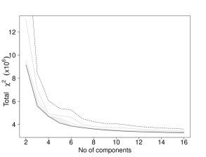
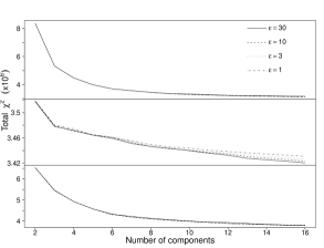
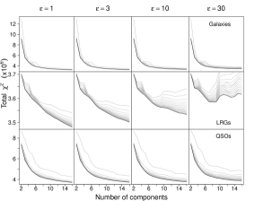
Using a number of spectra equal to the number of pixels selected for each source, we performed PCA on those data. As described in Section 4, the training data were first projected into a hyperplane orthogonal to the mean spectrum that is passing from the zero point. To do so each spectrum was scaled appropriately and the mean spectrum was subtracted from it. Additionally, the flux in each spectral bin was divided with the RMS of the error in that pixel for all the non-masked pixels in the training sample. The PCA results were used as an initialization to our method. HMF was trained with a subset of approximately 1000 spectra of each type, for a different number of components and for 16 iterations, which seems to be enough for the method to reach convergence. This can be seen in Figure 1 in which we present the results of the fitting (total $\chi^{2}$, that is, the sum of $\chi^{2}$ values over all wavelengths and all spectra) of the 1000 spectra of our sample for a different number of components. This test was also performed for four different values (1,3,10 and 30) of the smoothing factor $\epsilon$.

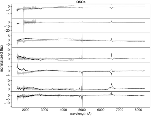
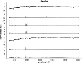
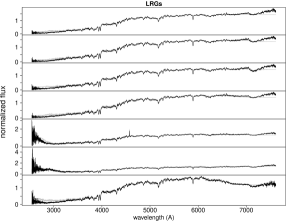
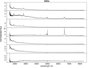
In Figure 1 we can see that the fitting of the spectra improves a lot even after the first iteration, indicating that for a given number of components HMF can achieve a better modeling of the spectra than PCA (i.e. under the assumption that the likelihood is the best scalar, for a given number of components HMF can achieve a higher-likelihood than PCA). In Figure 2 we present our new set of components plotted over the initial PCA components. We should point out that a straight comparison between the components extracted by the two methods is not meaningful since they span different subspaces of the observed data. A comparison between the methods can be achieved only by using the results of the fitting to a set of spectra. An example of such a comparison is shown in Figure 3 where both PCA and HMF components are used to fit the same set of SDSS galaxy spectra.

In Figure 1 we also present how the components and the total $\chi^{2}$ value change with the value of the smoothing factor $\epsilon$. As was expected, by increasing the value of $\epsilon$ we impose more constraints, which leads to smoother components at the cost of less accurate fits.

In the results presented above (Figure 1) we have used the same set of data to train as well as to test the method. As a first step towards cross-validation we used a new random set of 1000 spectra as a testing set. The results of the fitting of this set, at each iteration, with the extracted HMF components (when HMF is trained with the same set of spectra as before), are presented in Figure 4. In these plots with different types of line we present the results for different values of $\epsilon$. As we can see in the new test set, the best fit is achieved by different values of $\epsilon$ and not for the smallest one as before.

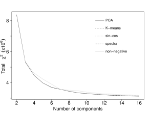
In order to check how much the method depends on the initialization we repeated our tests using different sets of components as our initial basis. In Figure 5 we present the results of the fitting for the same test set as before when a random set of spectra, the output of the K-means algorithm and a set of sin and cosin functions were used to initialize the training of HMF. More specifically, in the case that a set of random spectra was used, we selected the ones that include data at the reddest or the bluest wavelengths. In the case of the K-means initialization, we used the algorithm kmeans(stats) implemented in R with a number of centers equal to the number of components. The algorithm uses a random set of points as its initialization and therefore the results are slightly different in every run.

By comparing these results we see that they are becoming worse as we change the initialization from the PCA output, to the random spectra, to the K-means results and to the sin and cosin functions. This result is expected since the PCA results are chosen in a way to increase the percentage of the total variance they include. The most probable reason why the random spectra seem to be a better initialization than the K-means output is that we have chosen spectra that include information at the ends of the wavelength coverage, something that is probably not true in the K-means initialization where the centers are defined mainly by spectra with constant values in these areas. The sin and cosin functions lead to the worst results as expected since they include the least information compared to all the other initializations used here.

As a last test of the method we checked how a non-negative constraint affects the results. Since negative values in the spectra are caused by observational errors, modeling the spectra of astronomical sources with components that include negative values has no physical meaning. This problem can be solved be applying a non-negative constraint to our basis. The way that this is achieved is by initializing with a non-negative set of components and coefficients and iterating according to the non-negative a-step of equation (15) and the non-negative g-step of equation (16). One of the best ways to initialize this method with a set of non-negative components that include physical information is to use once again the K-means algorithm. The results of the fitting of the test set of spectra with the components extracted in this way after 2048 iterations are presented in Figure 5, while in Figure 6 we present the resulting components for each type of object for $K=7$.

By comparing those results with the ones obtained without the non-negative constraint we see that the fitting is now worse. This was expected since non-negativity is a very strict constraint. On the other hand even if the components now seem to have a better physical meaning, that is, they look more like spectra of particular type of objects, in many cases there seems to be a problem at the edges of the spectra where they tend to start from exactly zero values (for example, the components for LRG spectra). At this point we should mention that when applying the method for the non-negative case we have not used an additional smoothing constraint.

Based on the results presented here and an additional test, that is defining the minimum number of components required to detect the second redshifts in the SLACS and BHB candidate samples, we selected the optimal number of components and value of $\epsilon$. More specifically, we decided to fit the SDSS spectra using the 14, 7 and 14 components that were produced by HMF when trained with Main Galaxy, LRG and QSO spectra for 16 iterations and for $\epsilon$=3, 30 and 10 respectively. It is interesting that fewer components are needed in order to fit well the LRG SDSS spectra than the Main Galaxy and QSO spectra. This is expected, since the LRG spectra show very little variation (Eisenstein et al., 2003) in comparison to other types of sources like QSOs (Yip et al., 2004). A more detailed description of the fitting and its results is presented below.

5.2 Two-redshift models

In order to detect the presence of a second redshift in the SDSS spectra we compute the improvement of the fitting when a spectrum is fitted with two sets of componets at two different redshifts (that is, the one estimated by SDSS and another redshift) instead of only one set of components at the redshift provided by SDSS. This second redshift is scanning a regular grid of values selected to be uniform in a logarithmic scale, that is, in the same way as the wavelengths in SDSS. In this way moving to the next value of the redshift grid is equivalent to shifting the spectrum by one pixel. In practice the improvement of the fitting can be estimated by measuring the $\chi^{2}$ difference between the two fits ($\Delta\chi_{in}^{2}$):

$$\displaystyle\Delta\,\chi_{in}^{2} = \sum_{j=m}^{M^{\prime}}\frac{\left[f_{ij}-\sum_{k=1}^{K}a_{ik}\,g_{k}(\lambda_{j}/[1+z_{i}])\right]^{2}}{\sigma^{2}_{ij}}-$$ (19)

$$- \sum_{j=m}^{M^{\prime}}\frac{\left[f_{ij}-\sum_{k=1}^{K}a^{\prime}_{ik}\,g_{k}(\lambda_{j}/[1+z_{i}])-\sum_{k=1}^{K}\beta_{ik}\,g_{k}(\lambda_{j}/[1+z_{n}])\right]^{2}}{\sigma^{2}_{ij}}\quad,$$

where $m$ and $M^{\prime}$ are the first and last common pixels between the components when moved to the SDSS and the second redshift ($z_{i}$ and $z_{n}$ respectively). By definition an improvement of the fitting will result in a positive value of $\Delta\chi_{in}^{2}$. In the case that the spectrum has significant flux coming from a second object, we expect that there will be a peak in $\Delta\chi_{in}^{2}$ at a second redshift equal to the one of that object. The strength of the peak depends on the brightness and therefore the distance of the second object, the presence of emission lines in its spectrum and to some extent to the spectral coverage. As it is obvious the use of an additional set of componets always improves the fitting of the spectrum. However, this improvement is not significant and does not vary a lot for different values of the second redshift in the cases that the signature of a second object is not present in the spectrum. Finally, since we perform our search using the difference of the $\chi^{2}$ values between the two fits, values of $\Delta\chi_{in}^{2}$ that correspond to different second redshifts are directly comparable, despite the fact that they might correspond to different number of pixels in the fits.

5.3 Testing

5.3.1 The SLACS survey

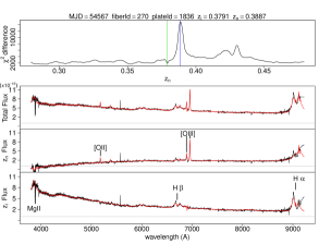
The SLACS survey (Bolton et al., 2008) includes 131 strong galaxy-galaxy gravitational lens candidates, selected by the presence of higher redshift emission lines on the top of a lower redshift stellar continuum. Using the components extracted by the method presented here (Section 5.1) for Main Galaxy and LRG SDSS spectra we applied the test described above (Section 5.2) in order to reproduce the results of the SLACS survey for the second redshift.

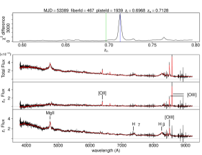
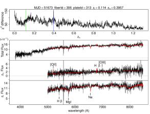
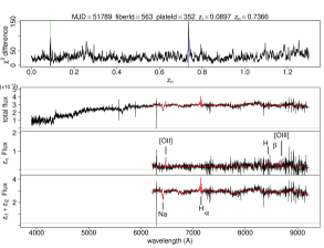
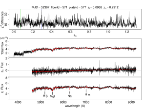
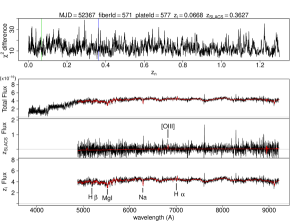
As a first step we applied the test using the 14 Main Galaxy components of Section 5.1 for both the foreground and the background object. For each spectrum of the SLACS survey we used the procedure described in Section 5.2 to search for peaks of $\Delta\,\chi_{in}^{2}$ corresponding to the second redshift. An additional criterion that we used was that the peaks (if present) should correspond to fits that did not produce negative [OIII] lines if they were included in the spectral range of the fit. In this way we detected peaks for 119 SLACS spectra at the same redshifts as those found in the SLACS survey (for an example, see Figure 8).

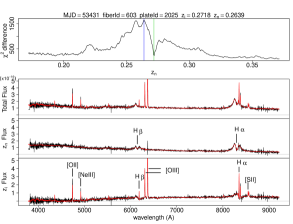
For the remaining 12 cases we applied the same procedure but this time using the LRG components to fit the foreground object and the Main Galaxy components to fit the background one. The results show that using this approach we were able to extract the same results as the SLACS survey for 6 of those spectra (an example is shown in Figure 9).

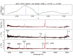
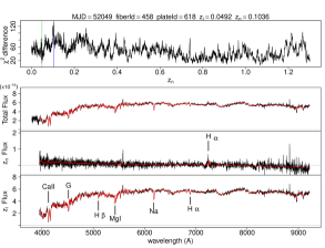
In the other 6 cases we detect a different second redshift than the one reported by Bolton et al. (2008). For those objects we applied once again our method but this time assuming the presence of three objects instead of two. More specifically, we fit the spectrum using a set of components (LRG or Main Galaxy) at the SDSS redshift, a set of components (Main Galaxy) at the second redshift to which was given the highest probability by our method, and a set of components (Main Galaxy) at a redshift scanning a regular grid of values. This time we managed to predict the SLACS second redshift for 4 additional objects (SDSS J1155+6237, SDSS J1618+4353, SDSS J1621+3931 and SDSS J1718+6424), (an example is shown in Figure 10). For at least two of these sources (SDSS J1618+4353 and SDSS J1718+6424) the presence of three objects was confirmed by high resolution HST imaging observations which showed that in these two cases the lens consists of two foreground galaxies (Bolton et al. 2006; Bolton et al. 2008).

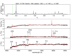
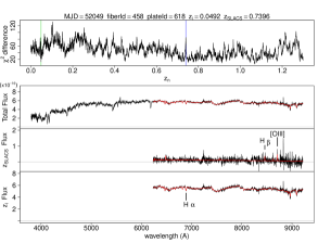
For only 2 (SDSS J1039+0513 and SDSS J1550+5258) out of the 131 spectra tested here we were not able to detect the second redshift. The results for these spectra as well as the fitting at the second redshift given by SLACS are shown in Figure 11. From this Figure it is clear that these are weak detections with no obvious signature of an additional object at the second redshift.

The results so far are very promising. Our goal is to apply this method to the whole SDSS spectroscopic sample in order to detect new gravitational lens candidates.

5.3.2 The known sample of BHB candidates

Another type of object that can be detected by the presence of two redshifts in its spectrum is the BHBs. In the case of BHBs we expect the presence of two sets of emission lines (one broad and one narrow) with a velocity shift between them, caused by the rotation of the less massive black hole around the more massive one that is located at the center of the system. Only four objects in SDSS had been selected to be BHB candidates until the completion of the tests presented here (Komossa et al., 2008; Bogdanovic, Eracleous & Sigurdsson, 2009; Dotti et al., 2009; Boroson & Lauer, 2009; Shields et al., 2009; Decarli et al., 2010). By applying our method to those spectra we followed the same procedure as in the case of gravitational lenses in order to test if we can detect the second redshift. However, since in this case the separation between the two sets of lines is expected to be small, we limited our search to redshift differences below 0.1. The second redshift can be either smaller or larger than the SDSS one.

The spectra were fitted using a set of QSO components that were extracted in Section 5.1 at the SDSS redshift and another set of the same components at a redshift scanning a narrow grid of regular values. The results for the four candidates are presented in Figure 7 where we can see that we are able to reproduce all of the four spectra with shifted broad lines given in the literature.

This method was applied to spectra of 54 586 and 3929 objects spectroscopically classified as QSOs and galaxies respectively in SDSS DR7, with 0.1$<$z$<$1.5 in order to detect more candidates of this type of object (Tsalmantza et al. 2011). The search resulted to 32 objects with peculiar spectra, nine of which can be interpreted as BHB candidates.

Section 6 Discussion

We have developed a new technique called “HMF” for dimensionality reduction, similar to PCA and other kinds of factor analysis, but based on optimization of a probabilistically justifiable objective function. The method produces—in principle—the $K$ components whose linear combination best reproduces well the whole training set of the observations, given the reported observational uncertainty variances. Because the method makes proper use of the observational uncertainties, it also deals properly with missing data; it does not require that each data point has a measurement on every axis, nor does it involve heuristic interpolation or patching of those missing data.

Since HMF is based on the minimization of a total $\chi^{2}$—unlike PCA, which is based on maximization of the observed data variance captured by the top components—it produces basis functions that fit the real data much better than the PCA results, for the same number $K$ of components, essentially by construction. In contrast to PCA, HMF is also able to extract more information from the training set because it uses many data points that could not be used with PCA, and more data dimensions or directions per data point. An example of this is that we managed to achieve maximum wavelength coverage in the HMF-generated components even though the training set included objects in a large range of redshifts, not one of which has data over the full wavelength range. PCA has one advantage over HMF, and that is speed. Even though the individual HMF $\chi^{2}$ minimization iterations steps are fast, the number of iterations make the method still much slower than PCA. This is the price of probabilistic righteousness.

At this point it is responsible to note that the “a-step, g-step” formalisms presented here represent only one choice among many for optimization: Specialists in optimization might point out that this iterative scheme is itself heuristic, and there might be far faster methods that could be found by good non-linear least-squares optimization systems. Along these lines, all derivatives of the bilinear model are easy to compute analytically.

Perhaps the biggest advantage of HMF over PCA is that, because it makes proper use of the errors, it does not require a high signal-to-noise data set for training. Because PCA models observed variance, at low signal-to-noise it captures the noise rather than the signal. HMF will not have this property, at least in the limit of large numbers. Having said that, we should mention that this does not mean that intersting results cannot be obtained by applying PCA to low signal-to-noise data. As an example we refer to the Boroson & Lauer (2010) study, where the authors have successfully identified a number of outlier sources (including a BHB candidate) using SDSS low signal-to-noise spectra.

We applied the HMF method to spectra from the SDSS, building a data-driven model of the spectra over a wide wavelength range. This model does an excellent job of explaining the spectra even with a small number $K$ of components. The number of components K that is required to sufficiently model the data in each case, depends on the training set used by the method, e.g. its dimensionality $M$, the variance that it includes, the rank of its subspace etc. In order to choose the optimal number $K$ of components a kind of cross-validation was employed: The method is trained on a training set of spectra with different values of $K$; the trained components are used to fit a test set of observed spectra not in the training set.

For the training part of the method we use a subset of the observed spectra to which we want to apply the results. One way to improve the results presented here would be to use the whole set of spectra, except the one under testing, in order to train the method. However, this requires some engineering in the case of large surveys like SDSS, and for that reason we choose to use a subsample of the data for training purposes.

Another way to improve the results would be to add prior information on the amplitudes. Based on the coefficients extracted by the fitting of the training spectra by the components, we can draw conclusions about the real amplitudes that are likely to occur in the world of real astronomical spectra. Hierarchically inferred priors in amplitude space would improve performance at low signal-to-noise, and make the method more sensitive to outliers and unrealistic solutions. However, this also requires significant engineering that goes beyond the scope of the present work.

Another disadvantage of HMF relative to PCA is the existence of many local optima—HMF is not convex. This issue can be ameliorated by using different initializations and finding the local optima that produce the best fit to the test data. Also, because there are multiple optima that differ only by permutations and linear combinations of the same basis spectra (there are subspace-description degeneracies), comparisons among resulting components extracted from different initializations (or different methods) shouldn’t be performed by straight comparison between the components themselves; different solutions ought to be compared in the data space, or in the quality of the fit to a good test set of real data.

An additional advantage of HMF over PCA is that it also provides an option for non-negative and smoothness constraints in the resulting components and coefficients. This option can help produce results that do not include unphysical features (for example, negative emission lines or features smaller in scale than the spectrograph resolution). We should keep in mind though that if applied inappropriately, these constraints can have a big impact in the results and produce a poorer fit to the observed spectra.

The model is excellent for anomaly detection: We applied the HMF model produced with the SDSS training set to the problem of confirming double-redshift objects. Of the 131 galaxy–galaxy gravitational lenses in the SLACS survey we were able to automatically detect 129, using components trained on the SDSS Main Galaxy and LRG spectra. The confirmation was made by fitting the spectra with a mixture of two sets of spectral model components, one at the SDSS redshift and one at a second redshift; the quality of fit was compared to a single-redshift fits. In a similar manner, we were able to recover a set of four previously known black-hole binary candidates. In the future, we plan to perform comprehensive automatic searches for objects of these types in the entire SDSS spectroscopic data set.

Another application of the HMF method could be for the determination of more accurate redshifts for single objects. This application could be very interesting for the case of QSOs at high redshifts, where narrow lines don’t appear in the observed optical spectral domain, and for defining template spectra for redshift estimation of objects that are going to be observed at low signal-to-noise in future surveys; by construction the method produces the best possible model of the objects under study (when the training set is appropriate).

Finally, it is worth noting that nothing in the method is specific to spectral data—it could be applied to any data for which a linear model makes sense—and nothing is specific to the delta-function basis of “spectral pixels”. The method produces a linear model; this can be passed through any linear basis functions (as it is in Blanton & Roweis 2007). Some such transformations could lead to faster or better regularized results at essentially no cost.

Figure 1: The total $\chi^{2}$ value estimated by the fit of the training set of spectra by the components produced by the method vs. the number of components for each type of object (rows) and values of $\epsilon$ (columns).

Figure 2: The first 7 components for each type of object (Main Galaxies, LRGs and QSOs) as estimated by the PCA (grey lines) and the method presented here (black lines).

Figure 3: The total $\chi^{2}$ value (sum over all spectra and all pixels) estimated by the fit of a test set of SDSS galaxy spectra ($\approx$ 1000 objects) by the HMF (grey and black lines) and the PCA (dashed line) components vs. the number of components used in each case. From the top grey line to the bottom black one, the lines correspond to the results based on different successive iterations of the HMF (i.e. from iteration 1 to 16). It is clear that the HMF components can achieve a better fitting of the observations even from the first iteration of the method.

Figure 4: The total $\chi^{2}$ value estimated by the fit of the test set of spectra by the components produced by HMF vs. the number of components for each type of object (rows: Main Galaxies, LRGs and QSOs respectively). The different types of lines represent the different values of $\epsilon$ used in each case.

Figure 5: The total $\chi^{2}$ value estimated by the fit of the test set of Main Galaxy spectra by the components produced by HMF vs. the number of components. The different types of lines represent the different initializations used (PCA, K-means, random spectra and sin and cosin functions).

Figure 6: The first 7 components for each type of object (Main Galaxies, LRGs and QSOs) as estimated by the K-means (grey lines) and the method presented here (black lines) when non-negative constraints were applied.

Figure 7: The four known BHB candidates. Top panel: The $\chi^{2}$ difference between the fitting of the spectrum with 1 and 2 sets of components. The green and blue lines represent the SDSS redshift ($z_{i}$) and the one with the largest $\chi^{2}$ difference ($z_{n}$). 2nd panel: The fitting of the spectrum (black) with both sets of components (red). 3rd panel: The part of the spectrum (black) fitted by the one set of components at the redshift with the highest $\chi^{2}$ difference (red). Bottom panel: The part of the spectrum (black) fitted by the one set of components at the SDSS redshift (red). The wavelength coverage of the fit in each panel (red line) is defined by the common area between the SDSS spectrum and the 2 sets of components when moved to the $z_{i}$ and $z_{n}$ redshifts.

Figure 8: As Figure 7 for an example of a lens candidate in the SLACS survey which was fitted with two sets of Main Galaxy components.

Figure 9: As Figure 7 for an example of a lens candidate in the SLACS survey which was fitted with one set of LRG components and one set of Main Galaxy components.

Figure 10: As Figure 7 for an example of lens candidate in the SLACS survey that was fitted with three sets of components (Main Galaxies). The bottom pannel shows the fitting of the residuals by two sets of components.

Figure 11: The 2 lens candidates in the SLACS survey that could not be confirmed by the method presented here. The left plots show the results of the fitting with the second set of components at the second redshift estimated with our method, while the right at the SLACS second redshift.

References

- Abazajian et al. (2009) Abazajian, K. N., et al., 2009, ApJS, 182, 543
- Akaike (1974) Akaike, H. 1974, IEEE Transactions on Automatic Control, 19, 716
- Allen et al. (2011) Allen, J. T., Hewett, P. C., Maddox, N., Richards, G. T., Belokurov, V. 2011, MNRAS, 410, 860
- Barrows et al. (2011) Barrows, R. S., Lacy, C. H. S., Kennefick, D., Kennefick, J., Seigar, M. S. 2011, NewA, 16, 122
- Blanton & Roweis (2007) Blanton, M. R. & Roweis, S. 2007, AJ, 133, 734
- Bolton et al. (2008) Bolton, A. S., Burles, S., Koopmans, L. V. E., Treu, T., Gavazzi, R., Moustakas, L., A., Wayth, R., Schlegel, D. J. 2008, ApJ, 682, 964
- Bolton et al. (2006) Bolton, A. S., Burles, S., Koopmans, L. V. E., Treu, T., Moustakas, L., A. 2006, ApJ, 638, 703
- Bogdanovic, Eracleous & Sigurdsson (2009) Bogdanovic, T., Eracleous, M., Sigurdsson, S. 2009, ApJ, 697, 288
- Boroson & Lauer (2010) Boroson, T. A., Lauer, T. R. 2010, AJ, 140, 390
- Boroson & Lauer (2009) Boroson, T. A., Lauer, T. R. 2009, Nature, 458, 53
- Boroson & Green (2009) Boroson, T. A., Green, R. F. 1992, ApJS, 80, 109
- Budavári et al. (2000) Budavári, T., Szalay, A. S., Connolly, A. J., Csabai, I., Dickinson, M. 2000, AJ, 120, 1588
- Budavári et al. (2009) Budavári, T., Wild, V., Szalay, A. S., Dobos, L., & Yip, C.-W. 2009, MNRAS, 394, 1496
- Chen et al. (2009) Chen, Y.-M., Wild, V., Kauffmann, G., Blaizot, J., Davis, M., Noeske, K., Wang, J.-M., Willmer, C. 2009, MNRAS, 393, 406
- Connolly & Szalay (1999) Connolly, A. J. & Szalay, A. S. 1999, AJ, 117, 2052
- Connolly et al. (2009) Connolly, A. J., Szalay, A. S., Bershady, M. A., Kinney, A. L., Calzetti, D. 1995, AJ, 110, 1071
- Decarli et al. (2010) Decarli, R., Dotti, M., Montuori, C., Liimets, T., Ederoclite, A. 2010, ApJ, 720L, 93
- Dotti et al. (2009) Dotti, M., Montuori, C., Decarli, R., Volonteri, M., Colpi, M., Haardt, F. 2009, MNRAS Letters, 398, 73
- Eisenstein et al. (2001) Eisenstein D. J., et al., 2001, AJ, 122, 2267
- Eisenstein et al. (2003) Eisenstein, D. J., et al., 2003, ApJ, 585, 694
- Eracleous et al. (2011) Eracleous, M., Boroson, T. A., Halpern, J. P., Liu, J. 2011, arXiv:1106.2952
- Ferreras et al. (2006) Ferreras, I., Pasquali, A., de Carvalho, R. R., de la Rosa, I. G., Lahav, O. 2006, MNRAS, 370, 828
- Francis et al. (1992) Francis, P. J., Hewett, P. C., Foltz, C. B., Chaffee, F. H. 1992, ApJ, 398, 476
- Glazebrook et al. (1998) Glazebrook, K., Offer, A. R., Deeley, K. 1998, ApJ, 492, 98
- Kitagawa & Gersch (1996) Kitagawa, G. & Gersch, W., 1996, Smoothness Priors Analysis of Time Series, Lecture Notes in Statistics 116 (Springer)
- Komossa et al. (2008) Komossa, S., Zhou, H., Lu, H. 2008, ApJ, 678, 81
- Nolan et al. (2006) Nolan, L. A., Harva, M. O., Kabán, A., Raychaudhury, S. 2006, MNRAS, 366, 321
- Suzuki et al. (2006) Suzuki, N. 2006, ApJS, 163, 110
- Rasmussen & Williams (2006) Rasmussen, C. E. & Williams, C., 2006, Gaussian Processes for Machine Learning (MIT Press)
- Richards et al. (2009) Richards, J. W., Freeman, P. E., Lee, A. B., Schafer, C. M. 2009, MNRAS, 399, 1044
- Roweis & Ghahramani (1999) Roweis, S. & Ghahramani, Z., 1999, Neural Computation, 11, 305
- Sanguinetti et al. (2005) Sanguinetti, G., Milo, M., Rattray, M., Lawrence, N. D. 2005, Bioinformatics, 21, 19, 3748
- Schwarz (1978) Schwarz, G. E. 1978, Annals of Statistics, 6, 461
- Shewchuk (1994) Shewchuk, J. R. 1994, http://www.cs.cmu.edu/q̃uake-papers/painless-conjugate-gradient.pdf
- Shields et al. (2009) Shields, G. A., Rosario, D. J., Smith, K. L., Bonning, E. W., Salviander, S., Kalirai, J. S., Strickler, R., Ramirez-Ruiz, E., Dutton, A. A., Treu, T., Marshall, P. J. 2009, ApJ, 707, 936
- Tsalmantza et al. (2011) Tsalmantza, P., Decarli, R., Dotti, M., Hogg, D. W. 2011, ApJ, 738, 20
- Vanderplas & Connolly (2009) Vanderplas, J., Connolly, A. 2009, AJ, 138, 1365
- Wentzell et al. (1997) Wentzell, P. D., Andrews, D. T., Hamilton, D. C., Faber, K., & Kowalski, B. R., 1997, Journal of Chemometrics, 11, 339
- Wild et al. (2007) Wild, V., Kauffmann, G., Heckman, T., Charlot, S., Lemson, G., Brinchmann, J., Reichard, T., Pasquali, A. 2007, MNRAS, 381, 543
- Wilson & Ghahramani (2011) Wilson, A. G., Ghahramani, Z. 2011, http://uai.sis.pitt.edu/papers/11/p736-wilson.pdf
- Wilson et al. (2011) Wilson, A. G., Knowles, D. A., Ghahramani, Z. 2011, arXiv:1110.4411
- Yip et al. (2004) Yip, C. W., Connolly, A. J., Vanden Berk, D. E., Ma, Z., Frieman, J. A., SubbaRao, M., Szalay, A. S., Richards, G. T., Hall, P. B., Schneider, D. P., Hopkins, A. M., Trump, J., Brinkmann, J. 2004, AJ, 128, 2603
- Yip et al. (2004) Yip, C. W., Connolly, A. J., Szalay, A. S., et al. 2004, AJ, 128, 585
![[Uncaptioned image]](/html/1201.3370/assets/x2.png)
![[Uncaptioned image]](/html/1201.3370/assets/x3.png)