Entropy of dynamical social networks

Abstract

Human dynamical social networks encode information and are highly adaptive. To characterize the information encoded in the fast dynamics of social interactions, here we introduce the entropy of dynamical social networks. By analysing a large dataset of phone-call interactions we show evidence that the dynamical social network has an entropy that depends on the time of the day in a typical week-day. Moreover we show evidence for adaptability of human social behavior showing data on duration of phone-call interactions that significantly deviates from the statistics of duration of face-to-face interactions. This adaptability of behavior corresponds to a different information content of the dynamics of social human interactions. We quantify this information by the use of the entropy of dynamical networks on realistic models of social interactions.

Introduction

Networks Dorogovtsev:2003 ; Newman:2003 ; Boccaletti:2006 ; Caldarelli:2007 ; Barrat:2008 encode information in the topology of their interactions. This is the main reason why networks are ubiquitous in complexity theory and constitute the underlying structures of social, technological and biological systems. The information encoded in social networks Granovetter:1973 ; Wasserman:1994 is essential to build strong collaborations Newman:2001 that enhance the performance of a society, to build reputation trust and to navigate Kleinberg efficiently the networks. For these reasons social networks are small world WS with short average distance between the nodes but large clustering coefficient. Therefore to understand how social network evolve, adapt and respond to external stimuli, we need to develop a new information theory of complex social networks.

Recently, attention has been addressed to entropy measures applied to email correspondence Eckmann:2004 , static networks Bianconi:2008 ; Bianconi:2008b ; Anand:2009 and mobility patterns Song:2010 . New network entropy measures quantify the information encoded in heterogenous static networks Bianconi:2008 ; Anand:2009 . Information theory tools set the limit of predictability of human mobilitySong:2010 . Still we lack methods to assess the information encoded in the dynamical social interaction networks.

Social networks are characterized by complex organizational structures revealed by network community and degree correlations Fortunato . These structures are sometimes correlated with annotated features of the nodes or of the links such as age, gender, and other annotated features of the links such as shared interests, family ties or common work locations Palla:2007 ; Lehmann . In a recent work Bianconi:2009 it has been shown by studying social, technological and biological networks that the network entropy measures can assess how significant are the annotated features for the network structure.

Moreover social networks evolve on many different time-scales and relevant information is encoded in their dynamics. In fact social networks are highly adaptive. Indeed social ties can appear or disappear depending on the dynamical process occurring on the networks such as epidemic spreading or opinion dynamics. Several models for adaptive social evolution have been proposed showing phase transitions in different universality classes Bornholdt:2002 ; Marsili:2004 ; Holme:2006 ; MaxiSanMiguel:2008 . Social ties have in addition to that a microscopic structure constituted by fast social interactions of the duration of a phone call or of a face-to-face interaction. Dynamical social networks characterize the social interaction at this fast time scale. For these dynamical networks new network measures are starting to be defined Latora:2009 and recent works focus on the implication that the network dynamics has on percolation, epidemic spreading and opinion dynamics Holme:2005 ; Vazquez:2007 ; Havlin:2009 ; Isella:2011 ; Karsai:2011a .

Thanks to the availability of new extensive data on a wide variety of human dynamics Barabasi:2005 ; Eagle:2006 ; Rybski:2009 ; Amaral:2008 ; Amaral:2009 , human mobility Brockmann:2006 ; Gonzalez:2008 ; Song:2010 and dynamical social networks Onnela:2007 , it has been recently recognized that many human activities Vazquez:2007 are bursty and not Poissonian. New data on social dynamical networks start to be collected with new technologies such as of Radio frequency Identification Devices Cattuto:2010 ; Isella:2011 and Bluetooth Eagle:2006 . These technologies are able to record the duration of social interactions and report evidence for a bursty nature of social interaction characterized by a fat tail distribution of the duration of face-to face interactions. This bursty behavior of social networks Hui:2005 ; Scherrer:2008 ; Cattuto:2010 ; Isella:2011 ; Stehle:2010 ; Zhao:2011 is coexisting with modulations coming from periodic daily (circadian rhythms) or weakly patterns Karsai:2011b . The fact that this bursty behavior is observed also in social interaction of simple animals, in the motion of rodents Chialvo , or in the use of words Motter , suggests that the underlying origin of this behavior is dictated by the biological and neurological processes underlying the dynamics of the social interaction. To our opinion this problem remains open: How much can humans intentionally change the statistics of social interactions and the level of information encoded in the dynamics of their social networks, when they are interfacing with a new technology?

In this paper we try to address this question by studying the dynamics of interactions through phone calls and comparing it with face-to-face interactions. We show that the entropy of dynamical networks is able to quantify the information encoded in the dynamics of phone-call interactions during a typical week-day. Moreover we show evidence that human social behavior is highly adaptive and that the duration of face-to-face interaction in a conference follows a different distribution than duration of phone-calls. We therefore have evidence of an intentional capability of humans to change statistically their behavior when interfacing with the technology of mobile phone communication. Finally we develop a model in order to quantify how much the entropy of dynamical networks changes if we allow modifications in the distribution of duration of the interactions.

Results

Entropy of dynamical social networks

In this section we introduce the entropy of dynamical social networks as a measure of information encoded in their dynamics. Since we are interested in the dynamics of contacts we assume to have a quenched social network $G$ of friendships, collaborations or acquaintances formed by $N$ agents and we allow a dynamics of social interactions on this network. If two agents $i,j$ are linked in the network they can meet and interact at each given time giving rise to the dynamical social network under study in this paper. If a set of agents of size $N$ is connected through the social network $G$ the agents $i_{1},i_{2},\ldots i_{n}$ can interact in a group of size $n$. Therefore at any given time the static network $G$ will be partitioned in connected components or groups of interacting agents as shown in Fig 1. In order to indicate that a social interaction is occurring at time $t$ in the group of agents $i_{1},i_{2},\ldots,i_{n}$ and that these agents are not interacting with other agents, we write $g_{i_{1},i_{2},\ldots,i_{n}}(t)=1$ otherwise we put $g_{i_{1},i_{2},\ldots,i_{n}}(t)=0$. Therefore each agent is interacting with one group of size $n>1$ or non interacting (interacting with a group of size $n=1$). Therefore at any given time

$$\sum_{{\cal G}=(i,i_{2},\ldots,i_{n})|i\in{\cal G}}g_{i,i_{2},\ldots,i_{n}}(t)=1.$$ (1)

where we indicate with ${\cal G}$ an arbitrary connected subgraph of $G$. The history ${\cal S}_{t}$ of the dynamical social network is given by ${\cal S}_{t}=\{g_{i_{1},i_{2},\ldots,i_{n}}(t^{\prime})\,\forall t^{\prime}<t\}$. If we indicated by $p(g_{i_{1},i_{2},\ldots,i_{n}}(t)=1|{\cal S}_{t})$ the probability that $g_{i_{1},i_{2},\ldots,i_{n}}(t)=1$ given the story ${\cal S}_{t}$, the likelihood that at time $t$ the dynamical networks has a group configuration $g_{i_{1},i_{2},\ldots,i_{n}}(t)$ is given by

$${\cal L}=\prod_{{\cal G}}p(g_{i_{1},i_{2},\ldots,i_{n}}(t)=1|{\cal S}_{t})^{g_{i_{1},i_{2},\ldots,i_{n}}(t)}$$ (2)

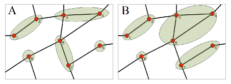
Figure 1: The dynamical social networks are composed by different dynamically changing groups of interacting agents. In panel (A) we allow only for groups of size one or two as it typically happens in mobile phone communication. In panel (B) we allow for groups of any size as in face-to-face interactions.

The entropy $S$ characterizes the logarithm of the typical number of different group configurations that can be expected in the dynamical network model at time $t$ and is given by $S=-\left\langle{\log{\cal L}}\right\rangle_{|{\cal S}_{t}}$ that we can explicitly express as

$$S=-\sum_{{\cal G}}p(g_{i_{1},i_{2},\ldots,i_{n}}(t)=1|{\cal S}_{t})\log p(g_{i_{1},i_{2},\ldots,i_{n}}(t)=1|{\cal S}_{t}).$$ (3)

According to the information theory results Cover:2006 , if the entropy is vanishing, i.e. $S=0$ the network dynamics is regular and perfectly predictable, if the entropy is larger the number of future possible configurations is growing and the system is less predictable. If we model face-to-face interactions we have to allow the possible formation of groups of any size, on the contrary, if we model the mobile phone communication, we need to allow only for pairwise interactions. Therefore, if we define the adjacency matrix of the network $G$ as the matrix $a_{ij}$, the log likelihood takes the very simple expression given by

$${\cal L}=\prod_{i}p(g_{i}(t)=1|{\cal S}_{t})^{g_{i}(t)}\prod_{ij|a_{ij}=1}p(g_{ij}(t)=1|{\cal S}_{t})^{g_{ij}(t)}$$ (4)

with

$$g_{i}(t)+\sum_{j}a_{ij}g_{ij}(t)=1,$$ (5)

for every time $t$. The entropy is then given by

$$S = -\sum_{i}p(g_{i}(t)=1|{\cal S}_{t})\log p(g_{i}(t)=1|{\cal S}_{t})$$ (6)

$$-\sum_{ij}a_{ij}p(g_{ij}(t)=1|{\cal S}_{t})\log p(g_{ij}(t)=1|{\cal S}_{t}).$$

Social dynamics and entropy of phone call interactions

We have analyzed the call sequence of subscribers of a major euroepan mobile service provider. We considered calls between users who at least once called each other during the examined $6$ months period in order to examine calls only reflecting trusted social interactions. The resulted event list consists of $633,986,311$ calls between $6,243,322$ users. For the entropy calculation we selected $562,337$ users who executed at least one call per a day during a week period. First of all we have studied how the entropy of this dynamical network is affected by circadian rhythms. We assign to each agent $i=1,2$ a number $n_{i}=1,2$ indicating the size of the group where he/she belongs. If an agent $i$ has coordination number $n_{i}=1$ he/she is isolated, and if $n_{i}=2$ he/she is interacting with a group of $n=2$ agents. We also assign to each agent $i$ the variable $t_{i}$ indicating the last time at which the coordination number $n_{i}$ has changed. If we neglect the feature of the nodes, the most simple transition probabilities that includes for some memory effects present in the data, is given by a probability $p_{n}=p_{n}(\tau,t)$ for an agent in state $n$ at time $t$ to change his/her state given that he has been in his/her current state for a duration $\tau=t-t_{i}$.

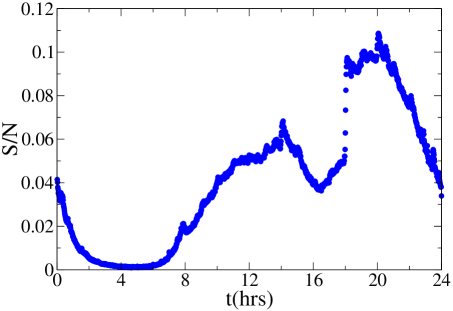
Figure 2: Mean-field evaluation of the entropy of the dynamical social networks of phone calls communication in a typical week-day. In the nights the social dynamical network is more predictable.

We have estimated the probability $p_{n}(\tau,t)$ in a typical week-day. Using the data on the probabilities $p_{n}(\tau,t)$ we have calculated the entropy, estimated by a mean-field evaluation (Check Text S1) of the dynamical network as a function of time in a typical week-day. The entropy of the dynamical social network is reported in Fig. 2. It significantly changes during the day describing the fact that the predictability of the phone-call networks change as a function of time. In fact, as if the entropy of the dynamical network is smaller and the network is an a more predictable state.

Adaptive dynamics face-to face interactions and phone call durations

In this section we report evidence of adaptive human behavior by showing that the duration of phone calls, a binary social interactions mediated by technology, show different statistical features respect to face-to-face interactions. The distributions of the times describing human activities are typically broad Barabasi:2005 ; Vazquez:2007 ; Hui:2005 ; Rybski:2009 ; Cattuto:2010 ; Isella:2011 , and are closer to power-laws, which lack a characteristic time scale, than to exponentials. In particular in Cattuto:2010 there is reported data on Radio Frequency Identification devices, with temporal resolution of 20s, showing that both distribution duration of face-to-face contacts and inter-contact periods is fat tailed during conference venues.

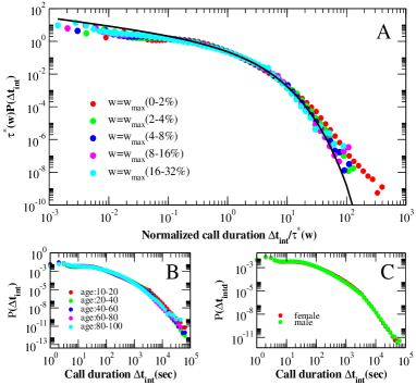
Figure 3: Probability distribution of duration of phone-calls. (A) Probability distribution of duration of phone-calls between two given persons connected by a link of weight $w$. The data depend on the typical scale $\tau^{\star}(w)$ of duration of the phone-call. (B) Probability distribution of duration of phone calls for people of different age. (C) Probability distribution of duration of phone-calls for people of different gender. The distributions shown in the panel (B) and (C) do not significantly depend on the attributes of the nodes.

Table 1: Typical times $\tau^{\star}(w)$ used in the data collapse of Fig. 3.

Weight of the link	Typical time $\tau^{\star}(w)$ in seconds (s)
(0-2%) $w_{max}$	111.6
(2-4%) $w_{max}$	237.8
(4-8%) $w_{max}$	334.4
(8-16%) $w_{max}$	492.0
(16-32%) $w_{max}$	718.8

Here we analysed the above defined mobile-call event sequence performing the measurements on all the users for the entire 6 months time period. The distribution of phone-call durations strongly deviates from a fat-tail distribution. In Fig. 3 we report this distributions and show that these distributions depend on the strength $w$ of the interactions (total duration of contacts in the observed period) but do not depend on the age, gender or type of contract in a significant way. The distribution $P^{w}(\Delta t_{in})$ of duration of contacts within agents with strenght $w$ is well fitted by a Weibull distribution

$$\tau^{*}(w)P^{w}(\Delta t_{in})=W_{\beta}\left(x=\frac{\Delta t}{\tau^{\star}(w)}\right)=\frac{1}{x^{\beta}}e^{-\frac{1}{1-\beta}x^{1-\beta}}.$$ (7)

with $\beta=0.47..$. The typical times $\tau^{*}(w)$ used for the data collapse of Figure 3 are listed in Table 1. The origin of this significant change in behavior of humans interactions could be due to the consideration of the cost of the interactions (although we are not in the position to draw these conclusions (See Fig. 4 in which we compare distribution of duration of calls for people with different type of contract) or might depend on the different nature of the communication. The duration of a phone call is quite short and is not affected significantly by the circadian rhythms of the population. On the contrary the duration of no-interaction periods is strongly affected by periodic daily of weekly rhythms. The distribution of no-interaction periods can be fitted by a double power-law but also a single Weibull distribution can give a first approximation to describe $P(\Delta t_{no}).$ In Fig. 5 we report the distribution of duration of no-interaction periods in the day periods between 7AM and 2AM next day. The typical times $\tau^{*}(k)$ used in Figure 5 are listed in Table 2.

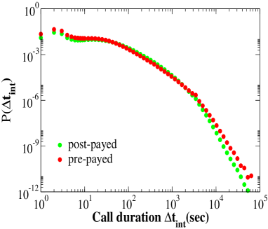
Figure 4: Probability distribution of duration of phone-calls for people with different types of contract. No significant change is observed that modifies the functional form of the distribution.

Discussion

The entropy of a realistic model of cell-phone interactions

The data on face-to-face and mobile-phone interactions show that a reinforcement dynamics is taking place during the human social interaction. Disregarding for the moment the effects of circadian rhythms and weakly patterns, a possible explanation of such results is given by mechanisms in which the decisions of the agents to form or leave a group are driven by memory effects dictated by reinforcement dynamics, that can be summarized in the following statements: i) the longer an agent is interacting in a group the smaller is the probability that he/she will leave the group; ii) the longer an agent is isolated the smaller is the probability that he/she will form a new group. In particular, such reinforcement principle implies that the probabilities $p_{n}(\tau,t)$ that an agent with coordination number $n$ changes his/her state depends on the time elapsed since his/her last change of state, i.e., $p_{n}(\tau,t)=f_{n}(\tau)$. To ensure the reinforcement dynamics any function $f_{n}(\tau)$ which is a decreasing function of its argument can be taken. In two recent papersStehle:2010 ; Zhao:2011 the face-to-face interactions have been realistically modelled with the use of the reinforcement dynamics, by choosing

$$f_{n}(\tau)=\frac{b_{n}}{(\tau+1)}.$$ (8)

with good agreement with the data when we took $b_{n}=b_{2}$ for $n\geq 2$ and $b_{1}>0$, $b_{2}>0$.

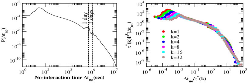
Figure 5: Distribution of non-interaction times in the phone-call data. The distribution strongly depends on circadian rhythms. The distribution of rescaled time depends strongly on the connectivity of each node. Nodes with higher connectivity $k$ are typically non-interacting for a shorter typical time scale $\tau^{\star}(k)$.

In order to model the phone-call data studied in this paper we can always adopt the reinforcement dynamics but we need to modify the probability $f_{n}(\tau)$ by a parametrization with an additional parameter $\beta\leq 1$. In order to be specific in our model of mobile-phone communication, we consider a system that consists of $N$ agents. Corresponding to the mechanism of daily cellphone communication, the agents can call each other to form a binary interaction if they are neighbor in the social network. The social network is characterized by a given degree distribution $p(k)$ and a given weight distribution $p(w)$. Each agent $i$ is characterized by the size $n_{i}=1,2$ of the group he/she belongs to and the last time $t_{i}$ he/she has changed his/her state. Starting from random initial conditions, at each timestep $\delta t=1/N$ we take a random agent. If the agent is isolated he/she will change his/her state with probability

$$f_{1}^{\beta}(\tau)=\frac{b_{1}}{(\tau+1)^{\beta}}$$ (9)

with $\tau=t-t_{i}$ and $b_{1}>0$. If he/she change his/her state he/she will call one of his/her neighbor in the social network which is still not engaged in a telephone call. A non-interacting neighbor agent will pick up the phone with probability $f_{1}^{\beta}(\tau^{\prime})$ where $\tau^{\prime}$ is the time he/she has not been interacting.

Table 2: Typical times $\tau^{\star}(k)$ used in the data collapse of Fig. 5.

Connectivity	Typical time $\tau^{\star}(k)$ in seconds (s)
k=1	158,594
k=2	118,047
k=4	69,741
k=8	39,082
k=16	22,824
k=32	13,451

If, on the contrary the agent $i$ is interacting, he/she will change his/her state with probability $f_{2}^{\beta}(\tau|w)$ depending on the weight of the link and on the duration of the phone call. We will take in particular

$$f_{2}^{\beta}(\tau|w)=\frac{b_{2}g(w)}{(\tau+1)^{\beta}}$$ (10)

where $b_{2}>0$ and $g(w)$ is a decreasing function of the weight $w$ of the link. The distributions $f_{1}^{\beta}(\tau)$ and $f_{2}^{\beta}(\tau|w)$ are parametrized by the parameter $\beta\leq 1$. As $\beta$ increases, the distribution of duration of contacts and duration of intercontact time become broader. These probabilities give rise to either Weibull distribution of duration of interactions (if $\beta<1$) or power-law distribution of duration of interaction $\beta=1$. Indeed for $\beta<1$, the probability $P^{w}_{2}(\tau)$ that a conversation between two nodes with link weight $w$ ends after a duration $\tau$ is given by the Weibull distribution (See Text S1 for the details of the derivation)

$$\tau^{*}(w)P^{w}_{2}(\tau)\propto W_{\beta}((\tau+1)/\tau^{\star}(w))$$ (11)

with $\tau^{\star}(w)=\left[{2b_{2}g(w)}\right]^{-1/(1-\beta)}$. This distribution well capture the distribution observed in mobile phone data and reported in Fig. 3 (for a discussion of the validity of the annealed approximation for predictions on a quenched network see the Text S1 ).

If, instead of having $\beta<1$ we have $\beta=1$ the probability distribution for duration of contacts is given by a power-law

$$P_{2}^{w}(\tau)\propto(\tau+1)^{-[2b_{2}g(w)+1]}.$$ (12)

This distribution is comparable with the distribution observed in face-to-face interaction during conference venues Stehle:2010 ; Zhao:2011 . The adaptability of human behavior, evident when comparing the distribution of duration of phone-calls with the duration of face-to-face interactions, can be understood as a possibility to change the exponent $\beta$ regulating the duration of social interactions.

Changes in the parameter $\beta$ correspond to a different entropy of the dynamical social network. Solving analytically this model we are able to evaluate the dynamical entropy as a function of $\beta$ and $b_{1}$. In Fig. 6 we report the entropy $S$ of the dynamical social network a function of $\beta$ and $b_{1}$ in the annealed approximation and the large network limit. In particular we have taken a network of size $N=2000$ with exponential degree distribution of average degree $\langle{k}\rangle=6$, weight distribution $P(w)=Cw^{-2}$ and function $g(w)=1/w$ and $b_{2}=0.05$. Our aim in Fig. 6 is to show only the effects on the entropy due to the different distributions of duration of contacts and non-interaction periods. Therefore we have normalized the entropy $S$ with the entropy $S_{R}$ of a null model of social interactions in which the duration of groups are Poisson distributed but the average time of interaction and non interaction time are the same as in the model of cell-phone communication. From Fig. 6 we observe that if we keep $b_{1}$ constant, the ratio $S/S_{R}$ is a decreasing function of the parameter $\beta$ indicating that the broader are the distribution of probability of duration of contacts the higher is the information encoded in the dynamics of the networks. Therefore the heterogeneity in the distribution of duration of contacts and no-interaction periods implies higher level of information in the social network. The human adaptive behavior by changing the exponent $\beta$ in face-to-face interactions and mobile phone communication effectively change the entropy of the dynamical network.

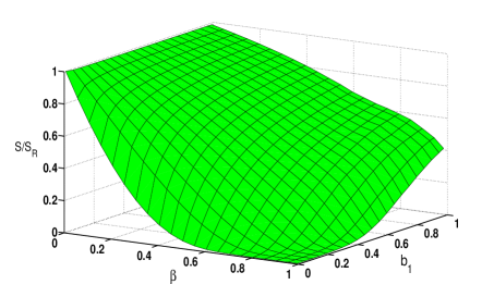
Figure 6: Entropy $S$ of social dynamical network model of pairwise communication normalized with the entropy $S_{R}$ of a null model in which the expected average duration of phone-calls is the same but the distribution of duration of phone-calls and non-interaction time are Poisson distributed. The network size is $N=2000$ the degree distribution of the network is exponential with average $\langle{k}\rangle=6$, the weight distribution is $p(w)=Cw^{-2}$ and $g(w)$ is taken to be $g(w)=b_{2}/w$ with $b_{2}=0.05$. The value of $S/S_{R}$ is depending on the two parameters $\beta,b_{1}$. For every value of $b_{1}$ the normalized entropy is smaller for $\beta\to 1$.

In conclusion, in the last ten years it has been recognized that the vast majority of complex systems can be described by networks of interacting units. Network theory has made tremendous progresses in this period and we have gained important insight into the microscopic properties of complex networks. Key statistical properties have been found to occur universally in the networks, such as the small world properties and broad degree distributions. Moreover the local structure of networks has been characterized by degree correlations, clustering coefficient, loop structure, cliques, motifs and communities. The level of information present in these characteristic of the network can be now studied with the tools of information theory. An additional fundamental aspect of social networks is their dynamics. This dynamics encode for information and can be modulated by adaptive human behavior. In this paper we have introduced the entropy of social dynamical networks and we have evaluated the information present in dynamical data of phone-call communication. By analysing the phone-call interaction networks we have shown that the entropy of the network depends on the circadian rhythms. Moreover we have shown that social networks are extremely adaptive and are modified by the use of technologies. The statistics of duration of phone-call indeed is described by a Weibull distribution that strongly differ from the distribution of face-to-face interactions in a conference. Finally we have evaluated how the information encoded in social dynamical networks change if we allow a parametrization of the duration of contacts mimicking the adaptability of human behavior. Therefore the entropy of social dynamical networks is able to quantify how the social networks dynamically change during the day and how they dynamically adapt to different technologies.

Material and Methods

In order to describe the model of mobile phone communication, we consider a system consisting of $N$ agents representing the mobile phone users. The agents are interacting in a social network $G$ representing social ties such as friendships, collaborations or acquaintances. The network $G$ is weighted with the weights indicating the strength of the social ties between agents. We use $N_{1}^{k}(t_{0},t)dt_{0}$ to denote the number of agents with degree $k$ that at time $t$ are not interacting and have not interacted with another agent since time $t^{\prime}\in(t_{0},t_{0}+{1}/{N})$. Similarly we denote by $N_{2}^{k,k^{\prime},w}(t_{0},t)dt_{0}$ the number of connected agents (with degree respectively $k$ and $k^{\prime}$ and weight of the link $w$) that at time $t$ are interacting in phone call started at time $t^{\prime}\in(t_{0},t_{0}+1/N)$. The mean-field equation for this model read,

$$\frac{\partial N_{1}^{k}(t_{0},t)}{\partial t}=-(1+ck){N_{1}^{k}(t_{0},t)}f_{1}(t_{0},t)+N\pi_{21}^{k}(t)\delta_{tt_{0}}$$

$$\frac{\partial N_{2}^{k,k^{\prime},w}(t_{0},t)}{\partial t}=-2N_{2}^{k,k^{\prime},w}(t_{0},t)f_{2}(t_{0},t|w)+N\pi_{12}^{k,k^{\prime},w}(t)\delta_{tt_{0}}$$ (13)

where the constant $c$ is given by

$$c=\frac{\sum_{k^{\prime}}\int_{0}^{t}dt_{0}N_{1}^{k^{\prime}}(t_{0},t)f_{1}(t_{0},t)}{\sum_{k^{\prime}}k^{\prime}\int_{0}^{t}dt_{0}N^{k^{\prime}}_{1}(t_{0},t)f_{1}(t_{0},t)}.$$ (14)

In Eqs. $(\ref{dN1w})$ the rates $\pi_{pq}(t)$ indicate the average number of agents changing from state $p=1,2$ to state $q=1,2$ at time $t$. These rates can be also expressed in a self-consistent way and the full system solved for any given choice of $f_{1}(t_{0},t)$ and $f_{2}(t_{0},t|w)$ (See Text S1 for details).

The definition of the entropy of dynamical social networks of a pairwise communication model, is given by Eq. (6). To evaluate the entropy of dynamical social network explicitly, we have to carry out the summations in Eq. $(6)$. These sums, will in general depend on the particular history of the dynamical social network, but in the framework of the model we study, in the large network limit will be dominated by their average value. In the following therefore we perform these sum in the large network limit. The first summation in Eq. $(6)$ denotes the average loglikelihood of finding at time $t$ a non-interacting agent given a history ${\cal S}_{t}$. We can distinguish between two eventual situations occurring at time $t$: (i) the agent has been non-interacting since a time $t-\tau$, and at time $t$ remains non-interacting; (ii) the agent has been interacting with another agent since time $t-\tau$, and at time $t$ the conversation is terminated by one of the two interacting agents.The second term in the right hand side of Eq. $(6)$, denotes the average loglikelihood of finding two agents in a connected pair at time $t$ given a history ${\cal S}_{t}$. There are two possible situations that might occur for two interacting agents at time $t$: (iii) these two agents have been non-interacting, and to time $t$ one of them decides to form a connection with the other one; (iv) the two agents have been interacting with each other since a time $t-\tau$, and they remain interacting at time $t$. Taking into account all these possibilities we have been able to use the transition probability form different state and the number of agents in each state to evaluate the entropy of dynamical networks in the large network limit (For further details on the calculation see the Text S1).

Ethics Statement

The dataset used in this study only involved de-identified information and no details about the subscribers were made available to us.

Entropy of dynamical networks
Supporting Informations
K. Zhao, M. Karsai and G. Bianconi

I The proposed model of cellphone communication

I.1 Dynamical social network for pairwise communication

We consider a system consisting of $N$ agents representing the mobile phone users. The agents are interacting in a social network $G$ representing social ties such as friendships, collaborations or acquaintances. The network $G$ is weighted with the weights indicating the strength of the social ties between agents. To model the mechanism of cellphone communication, the agents can call their neighbors in the social network $G$ forming groups of interacting agents of size two. Since at any given time a call can be initiated or terminated the network is highly dynamical. We assign to each agent $i=1,2,\dots,N$ a coordination number $n_{i}$ to indicate his/her state. If $n_{i}=1$ the agent is non-interacting, and if $n_{i}=2$ the agent is in a mobile phone connection with another agent. The dynamical process of the model at each time step $t$ can be described explicitly by the following algorithm:

• An agent $i$ is selected randomly at time $t$.

• The subsequent action of agent $i$ depends on his/her current state (i.e. $n_{i}$):

  • If $n_{i}=1$, he/she will call one of his/her non-interacting neighbors $j$ of $G$ with probability $f_{1}(t_{i},t)$ where $t_{i}$ denotes the last time at which agent $i$ has changed his/her state. Once he/she decides to call, agent $j$ will be chosen randomly in between the neighbors of $i$ with probability proportional to $f_{1}(t_{j},t)$, therefore the coordination numbers of agent $i$ and $j$ are updated according to the rule $n_{i}\rightarrow 2$ and $n_{j}\rightarrow 2$.

  • If $n_{i}=2$, he/she will terminate his/her current connection with probability $f_{2}(t_{i},t|w_{ij})$ where $w_{ij}$ is the weight of the link between $i$ and the neighbor $j$ that is interacting with $i$. Once he/she decides to terminate the connection, the coordination numbers are then updated according to the rule $n_{i}\rightarrow 1$ and $n_{j}\rightarrow 1$.

• Time $t$ is updated as $t\rightarrow t+1/N$ (initially $t=0$) and the process is iterated until $t=T_{max}$.

I.2 General solution to the model

In order to solve the model analytically, we assume the quenched network $G$ to be annealed and uncorrelated. Therefore we assume that at each time the network is rewired keeping the degree distribution $p(k)$ and the weight distribution $p(w)$ constant. Moreover we solve the model in the continuous time limit.Therefore we always approximate the sum over time-steps of size $\delta t=1/N$ by integrals over time. We use $N_{1}^{k}(t_{0},t)dt_{0}$ to denote the number of agents with degree $k$ that at time $t$ are not interacting and have not interacted with another agent since time $t^{\prime}\in(t_{0},t_{0}+{1}/{N})$. Similarly we denote by $N_{2}^{k,k^{\prime},w}(t_{0},t)dt_{0}$ the number of connected agents (with degree respectively $k$ and $k^{\prime}$ and weight of the link $w$) that at time $t$ are interacting in phone call started at time $t^{\prime}\in(t_{0},t_{0}+1/N)$. Consistently with the annealed approximation the probability that an agent with degree $k$ is called is proportional to its degree. Therefore the rate equations of the model are given by

$$\frac{\partial N_{1}^{k}(t_{0},t)}{\partial t} = -{N_{1}^{k}(t_{0},t)}f_{1}(t_{0},t)-ck{N_{1}^{k}(t_{0},t)}f_{1}(t_{0},t)+N\pi_{21}^{k}(t)\delta_{tt_{0}}$$

$$\frac{\partial N_{2}^{k,k^{\prime},w}(t_{0},t)}{\partial t} = -2N_{2}^{k,k^{\prime},w}(t_{0},t)f_{2}(t_{0},t|w)+N\pi_{12}^{k,k^{\prime},w}(t)\delta_{tt_{0}}$$ (15)

where the constant $c$ is given by

$$c=\frac{\sum_{k^{\prime}}\int_{0}^{t}dt_{0}N_{1}^{k^{\prime}}(t_{0},t)f_{1}(t_{0},t)}{\sum_{k^{\prime}}k^{\prime}\int_{0}^{t}dt_{0}N^{k^{\prime}}_{1}(t_{0},t)f_{1}(t_{0},t)}.$$ (16)

In Eqs. $(\ref{dN1w})$ the rates $\pi_{pq}(t)$ indicate the average number of agents changing from state $p=1,2$ to state $q=1,2$ at time $t$. These rates can be also expressed in a self-consistent way as

$$\pi_{21}^{k}(t) = \frac{2}{N}\sum_{k^{\prime},w}\int_{0}^{t}dt_{0}f_{2}(t_{0},t|w)N_{2}^{k,k^{\prime},w}(t_{0},t)$$

$$\pi_{12}^{k,k^{\prime},w}(t) = \frac{P(w)}{CN}\int_{0}^{t}dt_{0}\int_{0}^{t}dt_{0}^{\prime}N_{1}^{k}(t_{0},t)N_{1}^{k^{\prime}}(t_{0}^{\prime},t)f_{1}(t_{0},t)f_{1}(t^{\prime}_{0},t)(k+k^{\prime})$$ (17)

where the constant $C$ is given by

$$C=\sum_{k^{\prime}}\int_{0}^{t}dt_{0}k^{\prime}N^{k^{\prime}}_{1}(t_{0},t)f_{1}(t_{0},t).$$ (18)

The solution to Eqs. (15) is given by

$$N_{1}^{k}(t_{0},t)=N\pi_{21}^{k}(t_{0})e^{-(1+ck)\int_{t_{0}}^{t}{f_{1}(t_{0},t)}{}dt}$$

$$N_{2}^{k,k^{\prime},w}(t_{0},t)=N\pi_{12}^{k,k^{\prime},w}(t_{0})e^{-2\int_{t_{0}}^{t}{f_{2}(t_{0},t|w)}dt}$$ (19)

which must satisfy the self-consistent constraints Eqs. (17) and the conservation of the number of agents with different degree

$$\int dt_{0}\big{[}N_{1}^{k}(t_{0},t)+\sum_{k^{\prime},w}N_{2}^{k,k^{\prime},w}(t_{0},t)\big{]}=Np(k).$$ (20)

In the following we will denote by $P^{k}_{1}(t_{0},t)$ the probability distribution that an agent with degree $k$ is non-interacting for a period from $t_{0}$ to $t$ and by $P^{w}_{2}(t_{0},t)$ the probability that a connection of weight $w$ at time $t$ is active since time $t_{0}$. It is immediate to see that these distributions are given by the number of individual in a state $n=1,2$ multiplied by the probability of having a change of state, i.e.

$$P_{1}^{k}(t_{0},t) = (1+ck)f_{1}(t_{0},t)N_{1}^{k}(t_{0},t)$$

$$P_{2}^{w}(t_{0},t) = 2f_{2}(t_{0},t|w)\sum_{k,k^{\prime}}N_{2}^{k,k^{\prime},w}(t_{0},t).$$ (21)

I.3 Stationary solution with specific $f_{1}(t_{0},t)$ and $f_{2}(t_{0},t)$

In order to capture the behavior of the empirical data with a realistic model, we have chosen

$$f_{1}(t_{0},t) = f_{1}(\tau)=\frac{b_{1}}{(1+\tau)^{\beta}}$$

$$f_{2}(t_{0},t|w) = f_{2}(\tau|w)=\frac{b_{2}g(w)}{(1+\tau)^{\beta}}$$ (22)

with parameters $b_{1}>0$, $b_{2}>0$, $0\leq\beta\leq 1$ and arbitrary positive function $g(w)$. In Eqs. $(\ref{f2t})$, $\tau$ is the duration time elapsed since the agent has changed his/her state for the last time (i.e. $\tau=t-t_{0}$ ). The functions of $f_{1}(\tau)$ and $f_{2}(\tau|w)$ are decreasing function of their argument $\tau$ reflecting the reinforcement dynamics discussed in the main body of the paper. The function $g(w)$ is generally chosen as a decreasing function of $w$, indicating that connected agents with a stronger weight of link interact typically for a longer time. We are especially interested in the stationary state solution of the dynamics. In this regime we have that for large times $t\gg 1$ the distribution of the number of agents is only dependent on $\tau$. Moreover the transition rates $\pi_{pq}(t)$ also converge to a constant independent of $t$ in the stationary state. Therefore the solution of the stationary state will satisfy

$$N^{k}_{1}(t_{0},t) = N^{k}_{1}(\tau)$$

$$N^{k,k^{\prime},w}_{2}(t_{0},t) = N^{k,k^{\prime},w}_{2}(\tau)$$

$$\pi_{pq}(t) = \pi_{pq}.$$ (23)

The necessary condition for the stationary solution to exist is that the summation of self-consistent constraints given by Eq. (16) and Eq. (18) together with the conservation law Eq. (20) converge under the stationary assumptions Eqs. (23). The convergence depends on the value of the parameters $b_{0}$, $b_{1}$, $\beta$ and the choice of function $g(w)$. In particular, when $0\leq\beta<1$, the convergence is always satisfied. In the following subsections, we will characterize further the stationary state solution of this model in different limiting cases.

I.3.1 Case $0<\beta<1$

The expression for the number of agent in a given state $N_{1}^{k}(\tau)$ and $N_{2}^{k,k^{\prime},w}(\tau)$ can be obtained by substituting Eqs. (22) into the general solution Eqs. (19), using the stationary conditions Eqs. (23). In this way we get the stationary solution given by

$$N_{1}^{k}(\tau)=N\pi_{21}^{k}e^{\frac{b_{1}(1+ck)}{1-\beta}[1-(1+\tau)^{1-\beta}]}=N\pi_{21}^{k}m_{1}^{k}(\tau)$$

$$N_{2}^{k,k^{\prime},w}(\tau)=N\pi_{12}^{k,k^{\prime},w}e^{\frac{2b_{2}g(w)}{1-\beta}[1-(1+\tau)^{1-\beta}]}=N\pi_{12}^{k,k^{\prime},w}m_{2}^{w}(\tau).$$ (24)

To complete the solution is necessary to determine the constants $\pi_{21}^{k}$ and $\pi_{12}^{k,k^{\prime}w}$ in a self-consistent type of solution.To find the expression of $\pi_{12}^{k,k^{\prime},w}$ as a function of $\pi_{21}^{k}$ we substitute Eqs. $(\ref{N2w_tau})$ in Eq.$(\ref{pi12k_sum})$ and we get

$$\pi_{12}^{k,k^{\prime},w}(t) = \frac{1}{C}\pi_{21}^{k}P(w)\bigg{[}k\int_{0}^{t}dt_{0}m^{k}_{1}(t_{0},t)f_{1}(t_{0},t)\int_{0}^{t}dt_{0}^{\prime}N^{k^{\prime}}_{1}(t^{\prime}_{0},t)f_{1}(t^{\prime}_{0},t)$$ (25)

$$+ k^{\prime}\int_{0}^{t}dt_{0}m^{k}_{1}(t_{0},t)f_{1}(t_{0},t)\int_{0}^{t}dt_{0}^{\prime}N^{k^{\prime}}_{1}(t^{\prime}_{0},t)f_{1}(t^{\prime}_{0},t)\bigg{]}.$$

Finally we get a closed equation for $\pi_{21}^{k}$ by substituting Eq.(25) in Eq.(20) and using the definition of $c$ and $C$, given respectively by Eq. $(\ref{c_sum})$ and Eq. $(\ref{C_sum})$. Therefore we get

$$\pi_{21}^{k} \bigg{[} \int_{0}^{\infty}m^{k}_{1}(\tau)d\tau+\int_{w_{min}}^{w_{max}}P(w)\int_{0}^{\infty}m_{2}^{w}(\tau)d\tau dw$$ (26)

$$\times \bigg{(}ck\int_{0}^{\infty}m_{1}^{k}(\tau)f_{1}(\tau)d\tau+\int_{0}^{\infty}m_{1}^{k}(\tau)f_{1}(\tau)d\tau\bigg{)}\bigg{]}=p(k).$$

Performing explicitly the last two integrals using the dynamical solution given by Eqs. $(\ref{N2w_tau})$, this equation can be simplified as

$$\pi_{21}^{k}=\bigg{[}\int_{0}^{\infty}m^{k}_{1}(\tau)d\tau+\int_{w_{min}}^{w_{max}}P(w)\int_{0}^{\infty}m_{2}^{w}(\tau)d\tau dw\bigg{]}^{-1}p(k).$$ (27)

Finally the self-consistent solution of the dynamics is solved by expressing Eq. $(\ref{c_sum})$ by

$$c=\frac{\sum_{k}\pi_{21}^{k}(1+ck)^{-1}}{\sum_{k}\pi_{21}^{k}k(1+ck)^{-1}}.$$ (28)

Therefore we can use Eqs. $(\ref{pi10k})$ and $(\ref{cself})$ to compute the numerical value of $\pi_{21}^{k}$ and $c$. Inserting in these equations the expressions for $f_{1}(\tau),f_{2}(\tau|w)$ given by Eqs. $(\ref{f2t})$ and the solutions $N_{1}^{k}(\tau),N_{2}^{k,k^{\prime},w}(\tau)$ given by Eqs. $(\ref{N2w_tau})$ we get

$$P_{1}^{k}(\tau) \propto \frac{b_{1}(1+ck)}{(1+\tau)^{\beta}}e^{-\frac{b_{1}(1+ck)}{1-\beta}(1+\tau)^{1-\beta}}$$

$$P_{2}^{w}(\tau) \propto \frac{2b_{2}g(w)}{(1+\tau)^{\beta}}e^{-\frac{2b_{2}g(w)}{1-\beta}(1+\tau)^{1-\beta}}.$$ (29)

The probability distributions $P^{k}_{1}(\tau)$ and $P^{w}_{2}(\tau)$, can be manipulating performing a data collapse of the distributions, i.e.

$$\tau_{1}^{\star}(k)P_{1}^{k}\bigg{(}x_{1}=\frac{\tau}{\tau_{1}^{\star}(k)}\bigg{)} = A_{1}{x_{1}}^{-\beta}e^{-\frac{{x_{1}}^{1-\beta}}{1-\beta}}$$

$$\tau_{2}^{\star}(w)P_{2}^{w}\bigg{(}x_{2}=\frac{\tau}{\tau_{2}^{\star}(w)}\bigg{)} = A_{2}{x_{2}}^{-\beta}e^{-\frac{{x_{2}}^{1-\beta}}{1-\beta}}$$ (30)

with $\tau_{1}^{\star}(k)$ and $\tau_{2}^{\star}(w)$ defined as

$$\tau_{1}^{\star}(k) = \big{[}b_{1}(1+ck)\big{]}^{-\frac{1}{1-\beta}}$$

$$\tau_{2}^{\star}(w) = \big{[}2b_{2}g(w)\big{]}^{-\frac{1}{1-\beta}}$$ (31)

where $A_{1}$ and $A_{2}$ are the normalization factors. The data collapse defined by Eqs. (30) of the curves $P_{1}^{k}(\tau)$, $P^{w}_{2}(\tau)$ and are both described by Weibull distributions.

I.4 Comparisons with quenched simulations

To check the validity of our annealed approximation versus quenched simulations, we performed a computer simulation according to the dynamical process on a quenched network. In Fig. 7 we compare the results of the simulation with the prediction of the analytical solution. In particular in the reported simulation we have chosen $\beta=0.5$, $b_{1}=0.02$, $b_{2}=0.05$ and $g(w)=w^{-1}$, the simulation is based on a number of agent $N=2000$ and for a period of $T_{max}=10^{5}$, finally the data are averaged over $10$ realizations and the network is Poisson with average $\langle{k}\rangle=6$ and weight distribution $p(w)\propto w^{-2}$. In Fig. 7, we show evidence that the Weibull distribution and the data collapse of $P^{w}_{2}(\tau)$ well capture the empirical behavior observed in the mobile phone data (Fig. 3). The distribution of the non-interaction periods $P_{1}^{k}(\tau)$ in the model is by construction unaffected by circadian rhythms but follow a similar data collapse as observed in the real data (Fig. 5). The simulated data are also in good agreement with the analytical prediction predicted in the annealed approximation for the parameter choosen in the figure. As the network becomes more busy and many agents are in a telephone call, the quenched simulation and the annealed prediction of $P_{1}^{k}(\tau)$ differs more significantly.

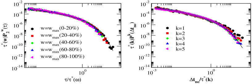
Figure 7: Data collapse of the simulation of the proposed model for cell phone communication. In the panel (A) we plot the probability $P_{2}^{w}(\tau)$ that in the model a pair of agents with strenght $w$ are interacting for a period $\tau$ and in the panel (B) we plot the probability $P_{1}^{k}(\tau)$ that in the model an agents of degree $k$ is non-interacting for a period $\tau$ The simulation data on a quenched networks are compared with the analytical predictions (solid lines) in the annealed approximation. The collapses data of $P_{2}^{w}(\tau)$ is described by Weibull distribution in agreement with the empirical results found in the mobile phone data.

I.4.1 Case $\beta=0$

For $\beta=0$ the functions $f_{1}(\tau)$ and $f_{2}(\tau|w)$ given by Eqs.$(\ref{f2t})$ reduce to constants, therefore the process of creation of an interaction is a Poisson process and no reinforcement dynamics is taking place in the network. Assigning $\beta=0$ to Eqs. (19), we get the solution

$$N_{1}^{k}(\tau) = N\pi_{21}^{k}e^{-b_{1}(1+ck)\tau}$$

$$N_{2}^{k,k^{\prime},w}(\tau) = N\pi_{12}^{k,k^{\prime},w}e^{-2b_{2}g(w)\tau}.$$ (32)

and consequently the distributions of duration of given states Eqs. $(\ref{P12})$ are given by

$$P_{1}^{k}(\tau)\propto e^{-b_{1}(1+ck)\tau}$$

$$P_{2}^{w}(\tau)\propto e^{-2b_{2}g(w)\tau}.$$ (33)

Therefore the probability distributions $P_{1}^{k}(\tau)$ and $P_{2}^{w}(\tau)$ are exponentials as expected in a Poisson process.

I.4.2 Case $\beta=1$

In this section, we discuss the case for $\beta=1$ such that $f_{1}^{k}(\tau)\propto(1+\tau)^{-1}$ and $f_{2}^{w}(\tau|w)\propto(1+\tau)^{-1}$. Using Eqs. (15) we get the solution

$$N_{1}^{k}(\tau)=N\pi_{21}^{k}(1+\tau)^{-b_{1}(1+ck)}$$

$$N_{2}^{k,k^{\prime},w}(\tau)=N\pi_{12}^{k,k^{\prime},w}(1+\tau)^{-2b_{2}g(w)}.$$ (34)

and consequently the distributions of duration of given states Eqs. $(\ref{P12})$ are given by

$$P_{1}^{k}(\tau)\propto\pi_{21}^{k}(1+\tau)^{-b_{1}(1+ck)-1}$$

$$P_{2}^{w}(\tau)\propto\pi_{12}^{k,k^{\prime},w}(1+\tau)^{-2b_{2}g(w)-1}.$$ (35)

The probability distributions are power-laws.This result remains valid for every value of the parameters $b_{1},b_{2},g(w)$ (See Ref. Zhao:2011 for a full account of the detailed solution of this model) nevertheless the stationary condition is only valid for

$$b_{1}(1+ck)>1$$

$$2b_{2}g(w)>1.$$ (36)

Indeed this condition ensures that the self-consistent constraits Eqs. (16), (18) and the conservation law Eq. (20) have a stationary solution.

I.5 Solution of the mean-field model on a fully connected network

Finally, we discuss the mean-field limit on the model in which every agent can interact with every other agent. In this case, social network is a fully connected network. Therefore we use $N_{1}(t_{0},t)$ and $N_{2}(t_{0},t)$ to denote the number of agents of the two different states respectively and the rate equations are then revised to

$$\frac{\partial N_{1}(t_{0},t)}{\partial t} = -2{N_{1}(t_{0},t)}f_{1}(t_{0},t)+N\pi_{21}(t)\delta_{tt_{0}}$$

$$\frac{\partial N_{2}(t_{0},t)}{\partial t} = -2{N_{2}(t_{0},t)}f_{2}(t_{0},t)+N\pi_{12}(t)\delta_{tt_{0}}$$ (37)

Since we will refer to this model only in the framework of a null model, we will only discuss the case in which the dynamics of the network is Poissonian, i.e. when

$$f_{1}(t_{0},t) = {b_{1}}$$

$$f_{2}(t_{0},t) = {b_{2}}.$$ (38)

The stationary solution of this model is given by exponentials, i.e.

$$N_{1}(\tau) = N\pi_{21}e^{-2b_{1}\tau}$$

$$N_{2}(\tau) = N\pi_{12}e^{-2b_{2}\tau}.$$ (39)

Finally the distributions of duration of given states expressed by Eqs. $(\ref{P12})$ are given by

$$P_{1}(\tau) \propto e^{-2b_{1}\tau}$$

$$P_{2}(\tau) \propto e^{-2b_{2}\tau},$$ (40)

which are exponential distributions as expected in a Poisson process.

II Entropy of the dynamical social networks

II.1 Entropy of the dynamical social networks of pairwise communication

The definition of the entropy of dynamical social networks of a pairwise communication model, is given by Eq. (6) of the main body of the article that we repeat here for convenience,

$${S}= - \sum_{i}P(g_{i}(t)=1|{\cal S}_{t})\log P(g_{i}(t)=1|{\cal S}_{t})$$ (41)

$$- \sum_{ij}a_{ij}P(g_{ij}(t)=1|{\cal S}_{t})\log P(g_{ij}(t)=1|{\cal S}_{t})$$

In this equation the matrix $a_{ij}$ is the adjacency matrix of the social network and $g_{ij}(t)=1$ indicates that at time $t$ the agents $i$ and $j$ are interacting while $g_{i}(t)=1$ indicates that agent $i$ is non-interacting.Finally ${\cal S}_{t}=\{g_{i}(t^{\prime}),g_{ij}(t^{\prime})\ \ \forall t^{\prime}<t\}$ indicates the dynamical evolution of the social network. In this section, we will evaluate the entropy of dynamical social networks in the framework of the annealed model of pairwise communication explained in detail in the previous section of this supplementary material. To evaluate the entropy of dynamical social network explicitly, we have to carry out the summations in Eq. $(\ref{s_pair})$. These sums, will in general depend on the particular history of the dynamical social network, but in the framework of the model we study, in the large network limit will be dominated by their average value. In the following therefore we perform these sum in the large network limit. The first summation in Eq. $(\ref{s_pair})$ denotes the average loglikelihood of finding at time $t$ a non-interacting agent given a history ${\cal S}_{t}$. We can distinguish between two eventual situations occurring at time $t$: (i) the agent has been non-interacting since a time $t-\tau$, and at time $t$ remains non-interacting; (ii) the agent has been interacting with another agent since time $t-\tau$, and at time $t$ the conversation is terminated by one of the two interacting agents. In order to characterize situation (i) we indicate by $P_{1\rightarrow 1}^{k}(\tau)$ the probability that a non-interacting agent with degree $k$ in the social network, that has not interacted since a time $\tau$, doesn’t change state. Similarly, in order to characterize situation (ii), we indicate by $P_{2\rightarrow 1}^{k,k^{\prime},w}(\tau)$ the probability that a connected pair of agents (with degrees $k$ and $k^{\prime}$ respectively, and weight of the link $w$) have interacted since time $\tau$ and terminate their conversation at time $t$. Given the stationary solution of the pairwise communication model, performed in the annealed approximation, the rates $P_{1\rightarrow 1}^{k}(\tau)$ and $P_{2\rightarrow 1}^{k,k^{\prime},w}(\tau)$ are given by

$$P_{1\rightarrow 1}^{k}(\tau) = 1-\frac{f_{1}(\tau)}{N}-\frac{kf_{1}(\tau)}{NC}\sum_{k^{\prime}}\int N^{k^{\prime}}_{1}(\tau^{\prime})f_{1}(\tau^{\prime})d\tau^{\prime}$$

$$= 1-(1+ck)\frac{f_{1}(\tau)}{N}$$

$$P_{2\rightarrow 1}^{k,k^{\prime},w}(\tau) = \frac{2f_{2}(\tau|w)}{N}$$ (42)

where the constant $C$ is given by

$$C=\sum_{k^{\prime}}\int k^{\prime}N^{k^{\prime}}_{1}(\tau^{\prime})f_{1}(\tau^{\prime})d\tau^{\prime}$$ (43)

and $f_{1}(\tau)$ and $f_{2}(\tau|w)$ are given in Sec. I.3. The variable $N^{k}_{1}(\tau)$ indicates the number of agents of connectivity $k$ noninteracting since a time $\tau$. This number can in general fluctuate but in the large network limit it converges to its mean-field value given by Eq. $(\ref{N2w_tau})$ The second term in the right hand side of Eq. $(\ref{s_pair})$, denotes the average loglikelihood of finding two agents in a connected pair at time $t$ given a history ${\cal S}_{t}$. There are two possible situations that might occur for two interacting agents at time $t$: (iii) these two agents have been non-interacting, and to time $t$ one of them decides to form a connection with the other one; (iv) the two agents have been interacting with each other since a time $t-\tau$, and they remain interacting at time $t$. To describe the situation (iii), we indicate by $P_{1\rightarrow 2}^{k,k^{\prime}}(\tau,\tau^{\prime})$ the probability that two non interacting agents, isolated since time $t-\tau$ and $t-\tau^{\prime}$ respectively, interact at time $t$. In order to describe situation (iv), we denote by $P_{2\rightarrow 2}^{k,k^{\prime},w}(\tau)$ the probability that two interacting agents, in interaction since a time $t-\tau$, remain interacting at time $t$. In the framework of the stationary annealead approximation of the dynamical network these probabilities are given by

$$P_{1\rightarrow 2}^{k,k^{\prime}}(\tau,\tau^{\prime}) = \frac{f_{1}(\tau)f_{1}(\tau^{\prime})}{NC}(k+k^{\prime})$$

$$P_{2\rightarrow 2}^{k,k^{\prime},w}(\tau) = 1-\frac{2f_{2}(\tau|w)}{N}.$$ (44)

Therefore, the entropy of dynamical social networks given by Eq. (41) can be evaluated in the thermodynamic limit, and in the annealed approximation, according to the expression

$${\cal S}= - \sum_{k}\int_{0}^{\infty}N_{1}^{k}(\tau)P^{k}_{1\rightarrow 1}(\tau)\log{P^{k}_{1\rightarrow 1}(\tau)}d\tau$$ (45)

$$- \sum_{k,k^{\prime},w}\int_{0}^{\infty}N_{2}^{k,k^{\prime},w}(\tau)P^{k,k^{\prime},w}_{2\rightarrow 1}(\tau)\log{P^{k,k^{\prime},w}_{2\rightarrow 1}(\tau)}d\tau$$

$$- \frac{1}{2}\sum_{k,k^{\prime}}\int_{0}^{\infty}\int_{0}^{\infty}N_{1}^{k}(\tau)N_{1}^{k^{\prime}}(\tau^{\prime})P^{k,k^{\prime}}_{1\rightarrow 2}(\tau,\tau^{\prime})\log{P^{k,k^{\prime}}_{1\rightarrow 2}(\tau,\tau^{\prime})}d\tau d\tau^{\prime}$$

$$- \frac{1}{2}\sum_{k,k^{\prime},w}\int_{0}^{\infty}N_{2}^{k,k^{\prime},w}(\tau)P^{k,k^{\prime},w}_{2\rightarrow 2}(\tau)\log{P^{k,k^{\prime},w}_{2\rightarrow 2}(\tau)}d\tau,$$

with $N_{1}^{k}(\tau)$ and $N_{2}^{k,k^{\prime},w}(\tau)$ given in the large network limit by Eqs. $(\ref{N2w_tau})$.

II.2 Entropy of the null model

To understand the impact of the distribution of duration of the interactions and of the distribution of non-interaction periods, we have compared the entropy $S$ of the pairwise communication model with the entropy $S_{R}$ of a null model. Here we use the exponential mean-field model described in Section I.5 as our null model. In this model the agents are embedded in a fully connected networks and the probability of changing the agent state does not include the reinforcement dynamics. In fact we have that the transition rates are independent of time ($\beta=0$) and given by $f^{R}_{1}(\tau)=b_{1}^{R}$ and $f^{R}_{2}(\tau)=b_{2}^{R}$. Following the same steps used in Sec. II.1 for evaluating $S$ in the model of pairwise communication on the networks, it can be easily proved that the entropy $S_{R}$ of the dynamical null model is given by

$$S_{R}= - \int_{0}^{\infty}N^{R}_{1}(\tau)\bigg{[}1-\frac{2b_{1}^{R}}{N}\bigg{]}\log{\bigg{[}1-\frac{2b_{1}^{R}}{N}\bigg{]}}d\tau$$ (46)

$$- \int_{0}^{\infty}N^{R}_{2}(\tau)\frac{2b_{2}^{R}}{N}\log{\frac{2b_{2}^{R}}{N}}d\tau$$

$$- \frac{1}{2}\int_{0}^{\infty}\int_{0}^{\infty}N^{R}_{1}(\tau)N^{R}_{1}(\tau^{\prime})\frac{2b_{1}^{R}}{NC^{R}}\log{\frac{2b_{1}^{R}}{NC^{R}}}d\tau d\tau^{\prime}$$

$$- \frac{1}{2}\int_{0}^{\infty}N_{2}^{R}(\tau)\bigg{[}1-\frac{2b_{2}^{R}}{N}\bigg{]}\log{\bigg{[}1-\frac{2b_{2}^{R}}{N}\bigg{]}}d\tau$$

where the constant $C^{R}$ is given by

$$C^{R}=\int_{0}^{\infty}N_{1}^{R}(\tau)d\tau,$$ (47)

and where $N_{1},N_{2}$ are given , in the large network limit by their mean-field value given by Eq.$(\ref{mfe})$. In order to build an appropriate null model for the pairwise communication model parametrized by $(\beta,b_{1},b_{2})$ ,we take the parameters of the null model $b_{1}^{R}$ and $b_{2}^{R}$ such that the proportion of the total number of agents in the two states (interacting or non-interacting) is the same in the pairwise model of social communication and in the null model. In order to ensure this condition we need to satisfy the following relation

$$\frac{\sum_{k}\int_{0}^{\infty}N_{1}^{k}(\tau)d\tau}{\sum_{k,k^{\prime},w}\int_{0}^{\infty}N_{2}^{k,k^{\prime},w}(\tau)d\tau}=\frac{\int_{0}^{\infty}N_{1}^{R}(\tau)d\tau}{\int_{0}^{\infty}N_{2}^{R}(\tau)d\tau}.$$ (48)

In particular we have chosen $b_{1}^{R}=b_{1}$ and we have used Eq. $(\ref{portion})$ to determine $b_{2}^{R}$.

III Measurement of the entropy of a typical week-day of cell-phone communication from the data

In this section we discuss the method of measuring the dynamical entropy from empirical cellphone data as a function of time $t$ in a typical weekday. This analysis gave rise to the results presented in figure $2$ in the main body of the paper. We have analyzed the call sequence of subscribers of a major European mobile service provider. We considered calls between users who at least once called each other during the examined $6$ months period in order to examine calls only reflecting trusted social interactions. The resulted event list consists of $633.986.311$ calls between $6.243.322$ users. For the entropy calculation we selected $562.337$ users who executed at least one call per a day during a working week period. Since the network is very large we have assumed that the dynamical entropy can be evaluate in the mean-field approximation. We measured the following quantities directly from the sample:

• $N_{1}(\tau,t)$ the number of agents in the sample that at time $t$ are not in a conversation since time $t-\tau$;

• $N^{calls}(\tau,t)$ the number of agents in the sample that are not in a conversation since time $t-\tau$ and make a call at time $t$;

• $N^{called}(\tau,t)$ the number of agents in the sample that are not in a conversation since time $t-\tau$ and are called at time $t$;

• $M^{in}(\tau,t)$ the number of agents that at time $t$ are in a conversation of duration $\tau$ with another agent in the sample;

• $M^{out}(\tau,t)$ the number of agents that at time $t$ are in a conversation of duration $\tau$ with another agent outside the sample;

• $M^{end}(\tau,t)$ the number of calls of duration $\tau$ that end at time $t$.

Using the above quantities, we estimated the probability $p^{calls}(\tau,t)$ that an agent makes a call at time $t$ after a non-interaction period of duration $\tau$, the probability $p^{called}(\tau,t)$ that an agent is called at time $t$ after a non-interaction period of duration $\tau$ and the probability $\pi(\tau,t)$ that a call of duration $\tau$ ends at time $t$,according to the following relations

$$p^{calls}(\tau,t) = \frac{N^{calls}(\tau,t)}{N_{1}(\tau,t)}$$

$$p^{called}(\tau,t) = \frac{N^{called}(\tau,t)}{N_{1}(\tau,t)}$$

$$\pi(\tau,t) = \frac{M^{end}(\tau,t)}{M^{in}(\tau,t)/2+M^{out}(\tau,t)}.$$ (49)

Since the sample of $562.337$ users we are considering is a subnetwork of the whole dataset constituted by $6.243.322$ users, in our measurement, an agent can be in one of three possible states

• state 1: the agent is non-interacting;

• state 2: the agent is in a conversation with another agent of the sample;

• state 3: the agent is in a conversation with an agent outside the sample.

Therefore , to evaluate the entropy of the data, we can modify Eq.(41) into

$${\cal S}(t)= - \sum_{i}P(g_{i}(t)=1|{\cal S}_{t})\log P(g_{i}(t)=1|{\cal S}_{t})$$ (50)

$$- \sum_{ij}a_{ij}P(g_{ij}(t)=1|{\cal S}_{t})\log P(g_{ij}(t)=1|{\cal S}_{t})$$

$$- \sum_{i}P(g^{\prime}_{i}(t)=1|{\cal S}_{t})\log P(g^{\prime}_{i}(t)=1|{\cal S}_{t})$$

where $a_{ij}$ is the adjacency matrix of the quenched social network, $g_{i}(t)=1$ indicates that the agent $i$ is in state 1, $g_{ij}(t)=1$ indicates that the agent is in state 2 interacting with agent $j$ and $g^{\prime}_{i}(t)=1$ indicates the agent $i$ is in state 3. Finally ${\cal S}_{t}=\{g_{i}(t^{\prime}),g_{ij}(t^{\prime})\ g^{\prime}_{i}(t)\ \ \forall t^{\prime}<t\}$ indicates the dynamical evolution of the social network. To explicitly evaluate Eq. (50) in the large network limit where we assume that the dependence on the particular history are vanishing, we sum over the loglikelihood of all transitions between different states using the same strategy in Sec.2, which is

$${\cal S}(t)= - \sum_{\tau}N_{1}(\tau,t)P_{1\rightarrow 1}(\tau,t)\log{P_{1\rightarrow 1}(\tau,t)}$$ (51)

$$- \sum_{\tau}M^{in}(\tau,t)P_{2\rightarrow 1}(\tau,t)\log{P_{2\rightarrow 1}(\tau,t)}$$

$$- \sum_{\tau}M^{out}(\tau,t)P_{3\rightarrow 1}(\tau,t)\log{P_{3\rightarrow 1}(\tau,t)}$$

$$- \frac{1}{2}\sum_{\tau,\tau^{\prime}}N_{1}(\tau,t)N_{1}(\tau^{\prime},t)P_{1\rightarrow 2}(\tau,\tau^{\prime},t)\log{P_{1\rightarrow 2}(\tau,\tau^{\prime},t)}$$

$$- \frac{1}{2}\sum_{\tau}M^{in}(\tau,t)P_{2\rightarrow 2}(\tau,t)\log{P_{2\rightarrow 2}(\tau,t)}$$

$$- \sum_{\tau}N_{1}(\tau,t)P_{1\rightarrow 3}(\tau,t)\log{P_{1\rightarrow 3}(\tau,t)}$$

$$- \sum_{\tau}M^{out}(\tau,t)P_{3\rightarrow 3}(\tau,t)\log{P_{3\rightarrow 3}(\tau,t)}.$$

where the probabilities of transitions between different states are given by

$$P_{1\rightarrow 1}(\tau,t) = 1-p^{calls}(\tau,t)-p^{called}(\tau,t)$$

$$P_{2\rightarrow 1}(\tau,t) = P_{3\rightarrow 1}(\tau,t)=\pi(\tau,t)$$

$$P_{1\rightarrow 2}(\tau,\tau^{\prime},t) = \frac{(1-\gamma)}{C}\bigg{[}p^{calls}(\tau,t)p^{called}(\tau^{\prime},t)+p^{calls}(\tau^{\prime},t)p^{called}(\tau,t)\bigg{]}$$

$$P_{2\rightarrow 2}(\tau,t) = P_{3\rightarrow 3}(\tau,t)=1-\pi(\tau,t)$$

$$P_{1\rightarrow 3}(\tau,t) = \gamma\bigg{[}p^{calls}(\tau,t)+p^{called}(\tau,t)\bigg{]}$$ (52)

and where $C$ is given by

$$C=\sum_{\tau}N_{1}(\tau,t)p^{called}(\tau,t).$$ (53)

Finally in 52 we have introduced a parameter $\gamma\in[0,1]$ to denote the portion of the calls occurring between an agent in the sample and an agent out of the sample. For simplicity, we assume that $\gamma$ is a constant. Substituting Eq.(52) into Eq.(51), we have performed the summation over $\tau$ to obtain the value of entropy as a function of $t$ presented in Figure 2 of the main body of the paper where we have taken $\gamma=0.8$, consistently with the data.

References

- (1) Dorogovtsev SN, Mendes JFF (2003) Evolution of networks: From biological nets to the Internet and WWW. Oxford Univ Press.
- (2) Newman MEJ (2003) The structure and function of complex networks. SIAM Rev 45: 157-256.
- (3) Boccaletti S, Latora V, Moreno Y, Chavez M, Hwang DU, et al. (2006) Complex networks: Structure and dynamics. Phys Rep 424: 175-308.
- (4) Caldarelli G (2007) Scale-Free Networks. Oxford Univ Press.
- (5) Barrat A, Barthélemy M, Vespignani A (2008). Dynamical processes on complex networks.
- (6) Granovetter M (1973) The strength in weak ties. Am J Socio 78: 1360-1380.
- (7) Wasserman S, Faust K (1994) Social Network Analysis: Methods and applications. Cambridge Univ Press.
- (8) Newman MEJ (2001) The structure of scientific collaboration networks. Proc Natl Acad Sci USA 98: 404-409.
- (9) Kleinberg JM (2000) Navigation in a small world. Nature 406: 845.
- (10) Watts DJ, Strogatz SH (1998) Collective dynamics of small-world networks. Nature 393: 440-442.
- (11) Eckmann JP, Moses E, Sergi D (2004) Entropy of dialogues creates coherent structures in e-mail traffic. Proc Natl Acad Sci USA 101: 14333.
- (12) Bianconi G (2008) The entropy of randomized network ensembles. Europhys Lett 81: 28005.
- (13) Bianconi G, Coolen ACC, Perez-Vicente CJ (2008) Entropies of complex networks with hierarchically constrained topologies. Phys Rev E 78: 016114.
- (14) Anand K, Bianconi G (2009) Entropy measures for networks: Toward an information theory of complex topologies. Phys Rev E 80: 045102.
- (15) Song C, Qu Z, Blumm N, Barabási AL (2010) Limits of predictability in human mobility. Science 327: 1018-1021.
- (16) Castellano C, Fortunato S, Loreto V (2009) Statistical physics of social dynamics. Rev Mod Phys 81: 591-646.
- (17) Palla G, Barabási AL, Vicsek T (2007) Quantifying social group evolution. Nature 446: 664-667.
- (18) Ahn YY, Bagrow JP, Lehmann S (2010) Link communities reveal multiscale complexity in networks. Nature 466: 761-764.
- (19) Bianconi G, Pin P, Marsili M (2009) Assessing the relevance of node features for network structure. Proc Natl Acad Sci USA 106: 11433-11438.
- (20) Davidsen J, Ebel H, Bornholdt S (2002) Emergence of a small world from local interactions: Modeling acquaintance networks. Phys Rev Lett 88: 128701.
- (21) Marsili M, Vega-Redondo F, Slanina F (2004) The rise and fall of a networked society: A formal model. Proc Natl Acad Sci USA 101: 1439-1442.
- (22) Holme P, Newman MEJ (2006) Nonequilibrium phase transition in the coevolution of networks and opinions. Phys Rev E 74: 056108.
- (23) Vazquez F, Eguíluz VM, San-Miguel M (2008) Generic absorbing transition in coevolution dynamics. Phys Rev Lett 100: 108702.
- (24) Tang J, Scellato S, Musolesi M, Mascolo C, Latora V (2009) Small-world behavior in time-varying graphs. Phys Rev E 81: 055101.
- (25) Holme P (2005) Network reachability of real-world contact sequences. Phys Rev E 71: 046119.
- (26) Vázquez A, Rácz B, Lukacs A, Barabàsi AL (2007) Impact of non-poissonian activity patterns on spreading processes. Phys Rev Lett 98: 158702.
- (27) Parshani R, Dickison M, Cohen R, Stanley HE, Havlin S (2009) Dynamic networks and directed percolation. Europhys Lett 90: 38004.
- (28) Isella L, Stehlé J, Barrat A, Cattuto C, Pinton JF, et al. (2011) What’s in a crowd? analysis of face-to-face behavioral networks. J Theor Biol 271: 166-180.
- (29) Karsai M, Kivelä M, Pan RK, Kaski K, Kertész J, et al. (2011) Small but slow world: How network topology and burstiness slow down spreading. Phys Rev E 83: 025102.
- (30) Barabási AL (2005) The origin of bursts and heavy tails in humans dynamics. Nature 435: 207-211.
- (31) Eagle N, Pentland AS (2006) Reality mining: sensing complex social systems. Personal Ubiquitous Comput 10: 255-268.
- (32) Rybski D, Buldyrev SV, Havlin S, Liljeros F, Makse HA (2009) Scaling laws of human interaction activity. Proc Natl Acad Sci USA 106: 12640-12645.
- (33) Malmgren RD, Stouffer DB, Motter AR, Amaral LA (2008) A poissonian explanation for heavy tails in e-mail communication. Proc Natl Acad Sci USA 105: 18153-18158.
- (34) Malmgren RD, Stouffer DB, Campanharo ASLO, Nunes-Amaral LA (2009) On universality in human correspondence activity. Science 325: 1696-1700.
- (35) Brockmann D, Hufnagel L, Geisel T (2006) The scaling laws of human travel. Nature 439: 462-465.
- (36) González MC, Hidalgo AC, Barabási AL (2008) Understanding individual human mobility patterns. Nature 453: 779-782.
- (37) Onnela JP, Saramäki J, Hyvönen J, Szabó G, Lazer D, et al. (2007) Structure and tie strengths in mobile communication networks. Proc Natl Acad Sci USA 104: 7332-7336.
- (38) Cattuto C, den Broeck WV, Barrat A, Colizza V, Pinton JF, et al. (2010) Dynamics of person-to-person interactions from distributed RFID sensor networks. PLoS ONE 5: e11596.
- (39) Hui P, Chaintreau A, Scott J, Gass R, Crowcroft J, et al. (2005) Pocket switched networks and human mobility in conference environments. In: Proceedings of the 2005 ACM SIGCOMM workshop on Delay-tolerant networking(Philadelphia, PA). pp. 244-251.
- (40) Borgnat ASP, Fleury E, Guillaume JL, Robardet C (2008) Description and simulation of dynamic mobility networks. Comp Net 52: 2842-2858.
- (41) Barrat JSA, Bianconi G (2010) Dynamical and bursty interactions in social networks. Phys Rev E 81: 035101.
- (42) Zhao K, Stehlé J, Bianconi G, Barrat A (2010) Social network dynamics of face-to-face interactions. Phys Rev E 83: 056109.
- (43) Jo HH, Karsai M, Kertész J, Kaski K (2011) Circadian pattern and burstiness in human communication activity. arXiv:11010377 .
- (44) Anteneodo C, Chialvo DR (2009) Unraveling the fluctuations of animal motor activity. Chaos 19: 033123.
- (45) Altmann EG, Pierrehumbert JB, Motter AE (2009) Beyond word frequency: Bursts, lulls, and scaling in the temporal distributions of words. PLoS ONE 4: e7678.
- (46) Cover T, Thomas JA (2006) Elements of Information Theory. Wiley-Interscience.

References

- (1) Zhao K, Stehlé J, Bianconi G, Barrat A (2011) Social network dynamics of face-to-face interactions. Phys Rev E 83:056109.