Nonequilibrium domain formation by pressure fluctuations

Fluctuations in thermal many-particle systems reflect fundamental dynamical processes in both equilibrium and nonequilibrium (NEQ) physics. In NEQ systems ritort fluctuations are important in a variety of contexts ranging from pattern formation hohenberg ; vdbroeck to molecular motors schaller ; kierfeld ; narayan ; prost . Here, we address the question if and how fluctuations may be employed to characterize and control pattern formation in NEQ nanoscopic systems. We report computer simulations of a liquid crystal system of prolate molecules (mesogens) sandwiched between flat walls, and exposed to a time-dependent external field. We find that a switchable smectic domain forms for sufficiently high frequency. Although pressure and temperature are too low to induce an equilibrium smectic phase, the fluctuations of the pressure in the NEQ steady state match the pressure fluctuations characteristic of the equilibrium smectic phase. Furthermore, the wall-normal pressure fluctuations give rise to a tangential “fluctuation-vorticity” tensor that specifies the symmetry-breaking direction of the smectic layers. Our calculations demonstrate a novel method through which nanomaterials with a high degree of molecular order may be manufactured in principle.

In nature, systems out of equilibrium are the rule and not the exception racz . Yet, only recently, with the growing interest in nano- and mesoscopic phenomena, NEQ thermodynamics has attracted a remarkably growing interest ritort ; seifert08 . Some profound and pioneering results are already available evans93 ; galla95 ; jarzin ; seifert05 , but a coherent picture of NEQ physics is still lacking.

A defining difference between the physics of NEQ and equilibrium systems is the presence of nonvanishing currents in the former, which are maintained by mechanical, thermal or chemical driving forceshohenberg ; schmiedl . In fact, many works zia ; hurtado_pre10 ; hurtado_pnas11 ; bertini ; derrida have addressed the statistical properties of these currents. Nonetheless, their physical role in a fluid is still not clear.

Here, we perform molecular dynamics simulations of $N=4000$ Gay-Berne-Kihara (GBK) molecules in presence of two atomically smooth flat walls. The GBK model has been successfully used to reproduce a typical equilibrium liquid crystal (LC) phase diagram for prolate mesogens martinez05 . The isobaric-isothermal ensemble was used to avoid unphysical stresses on the system due to the combination of a cubic simulation box and the formation of anisotropic phases.

The interaction of the molecules with the walls is modeled with a Lennard-Jones potential. Because of the presence of the walls the pressure in the system depends on the direction, that is, it is a second-rank tensor, and not a scalar

$$\boldsymbol{\mathcal{P}}\equiv\frac{1}{V}\sum_{i=1}^{N}\Big{[}m\mathbf{v}_{i}\otimes\mathbf{v}_{i}+\mathbf{r}_{i}\otimes\mathbf{f}_{i}\Big{]}$$ (1)

where $\mathbf{v}_{i}$ is the velocity of the $i$th particle, $m$ its mass, $\mathbf{r}_{i}$ its position vector, $\mathbf{f}_{i}$ the total force acting on it, $V$ the total volume of the system, and the operator $\otimes$ represents the dyadic product. Further, because of the planar geometry of the system, only the diagonal Cartesian components $\mathcal{P}_{xx},\mathcal{P}_{yy}$ and $\mathcal{P}_{zz}$ are nonzero, and the hydrostatic pressure is $P\equiv\langle\mathcal{P}_{xx}\rangle=\langle\mathcal{P}_{yy}\rangle$ (see Methods).

In the case of anisotropic molecules, it is important to specify their preferential alignment at the walls. A suitable quantity is the so-called “anchoring function” $g(\hat{\mathbf{u}})$ which discriminates energetically the orientation $\hat{\mathbf{u}}$ of a LC molecule with respect to a surface sonin , effectively defining a preferential direction, also called “easy axis” abbott11 . We consider a system confined by walls whose surface properties change periodically with time. Specifically, we give a temporal dependence to the anchoring function $g(\hat{\mathbf{u}},t)\equiv A\,(u_{x}V_{x}+u_{y}V_{y}+u_{z}V_{z})$, where $V_{x}=V_{y}=\sin(\omega t)$, $V_{z}=\cos(\omega t)$, $A$ is a constant, $\omega$ is the angular frequency of the sinusoidal external field, and $t$ is time. The effect of the external field is then to rotate the walls’ easy axes with time. The two easy axes rotate in phase. Time-dependent, responsive surfaces are a growing field of research stuart . Clare et al. clare06 have demonstrated that any specific anchoring of LCs can be selectively obtained by grafting semifluorinated organosilanes onto a surface. Further, the realization of time varying decorated surfaces has been reported where variable pH ionov04 ; matthews , electrochemical properties song , or UV-light irradiation are used as agents to effect the time dependence feng .

We present results for simulations in a range of temperature $T=4.0-6.0$ at fixed $P=3.6$ and investigate the behavior of the system as the period of the external field $\tau=2\pi/\omega$ is varied. We use dimensionless units throughout this work (see Methods). We first analyze the dependence of the energy fluctuations of the fluid on $\tau$. Figure 1 shows that $\langle(\Delta u_{ff})^{2}\rangle$ grows linearly with $\tau$ at large $\tau$ (which is the usual behavior of the energy fluctuations for a sinusoidal field). At $\tau\approx 7\times 10^{4}$ there is a crossover to a plateau. Because $\langle(\Delta u_{ff})^{2}\rangle$ is proportional to the specific heat of the fluid, this crossover reflects a structural rearrangement of the system occurring at small periods (high frequency).

Visual inspection of the molecular configurations reveals (Fig. 2a) that the molecules in the central portion of the fluid assemble in a well defined smectic domain (SD). This domain develops after a relatively small number of cycles of the external field and persists as long as the field is switched on; the SD disappears quickly once the external field is switched off. The fluid becomes heterogeneous. The molecules directly in contact with the walls rotate as the anchoring associated with the field changes. Between the contact layer at the walls and the SD there is a very turbulent layer, which does not show any spatial nor orientational order. Close observation of the molecular dynamics shows that individual molecules constantly leave this turbulent layer to join the SD or vice versa; however, the SD remains a stable feature. This is an instance of a nonequilibrium steady state (NESS). Only the molecules in the contact layer (i.e, the layer closest to the wall) are subject to direct interaction with the wall because of the short-range nature of the fluid-substrate potential $U_{fs}$ (see Fig. 2b and Methods). Therefore, the formation of SD must not be confused with a confinement effect, because the SD forms in the region where $U_{fs}\approx 0$. Hence, we believe the formation of the SD to be a general consequence of a time-dependent external field, irrespective of the precise realization of this field, so that our results are relevant to a broad class of physical situations.

Figure 1: Crossover of the energy fluctuations upon formation of a NESS. Dependence of the fluid-fluid energy fluctuations on the period of the external field $\tau$. The dashed lines represent linear fits for large and small values of $\tau$.

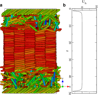
Figure 2: Molecular configuration of the simulated fluid and comparison with the extension of the fluid-substrate interaction. a, Snapshot showing the lateral view of the system in the $xz$-plane at $P=3.6$, $T=4.0$ and $\tau=3\times 10^{4}$. The molecules closest to the walls (top and bottom layers) rotate with the external field. A smectic domain is clearly visible in the center of the system. b, Plot of the fluid-substrate interaction $U_{fs}$ (see Methods) showing that it is effectively different from zero only in a region less than $5$ molecular diameter in size.

Now, a natural question to ask is: Why should a SD form? In equilibrium, the lowest $P$ for which a smectic phase forms at $T=4.0$ is more than twice the value of $P$ investigated in this work. Thus, the equilibrium phase transition is too far removed to play any role here. It is also important to note that even the local value of the pressure in the region where the SD forms is too low to explain a smectic state. The inset in Fig. 3 shows that the local pressure integrated over the SD volume, $\overline{\mathcal{P}}_{zz}$, is too low compared with the same quantity but calculated for an equilibrium smectic state at the same $P$ and $T$.

We then consider the temporal fluctuations of the pressure $\langle[\Delta\mathcal{P}_{zz}(z)]^{2}\rangle\equiv\langle[\mathcal{P}_{zz}(z,t)]^{2}\rangle-\langle[\mathcal{P}_{zz}(z,t)]\rangle^{2}$. Figure 3 shows the dependence of $\langle[\Delta\mathcal{P}_{zz}(z)]^{2}\rangle$ on the position along the $z$-axis. The confining walls are located at $z/L_{z}=\pm 1/2$, where the pressure fluctuations are very large due to the molecular rotation. As we move towards the center of the system, $\langle[\Delta\mathcal{P}_{zz}(z)]^{2}\rangle$ decreases rapidly until it reaches an almost constant value. It is the main observation of this study that when a SD forms the NEQ pressure fluctuations match the value of the equilibrium pressure fluctuations in a smectic phase

$$\langle[\Delta\mathcal{P}_{zz}(z)]^{2}\rangle_{\mathrm{NEQ}}=\langle[\Delta\mathcal{P}_{zz}(z)]^{2}\rangle_{\mathrm{EQ}}\,.$$ (2)

Also, the region of the plateau of $\langle[\Delta\mathcal{P}_{zz}(z)]^{2}\rangle$ coincides with the location of the SD. As $\tau$ increases the SD shrinks and becomes less coherent; this correlates very well with the behavior of $\langle[\Delta\mathcal{P}_{zz}(z)]^{2}\rangle$ in Fig. 3 for $\tau\geqslant 6\times 10^{4}$. This value deviates increasingly from $\langle[\Delta\mathcal{P}_{zz}(z)]^{2}\rangle_{\mathrm{EQ}}$.

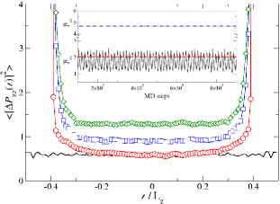
Figure 3: Normal pressure fluctuations. Dependence of the pressure tensor fluctuations on position along the $z$-axis for NEQ simulations at $P=3.6$, $T=4.0$ for $\tau=3\times 10^{4}$ ($\bigcirc$), $\tau=7\times 10^{4}$ ($\square$), and $\tau=9\times 10^{4}$ ($\Diamond$). The black line shows the value of the pressure tensor fluctuations for an equilibrium simulation in the smectic phase. Inset shows the local pressure integrated over the SD volume $\overline{\mathcal{P}}_{zz}$ ( ). The NEQ value oscillates with time following the external field, and, interestingly, its average value is close to the value characteristic of an equilibrium isotropic phase (       ), which is the thermodynamic equilibrium state at this $P$ and $T$. The equilibrium value characteristic of the smectic phase is much larger (  ​$\cdot$ ​  ​$\cdot$). From this we conclude that the local pressure is not large enough to drive the formation of a SD.

The instantaneous value of $\mathcal{P}_{zz}(z,t)$ may be treated as a stochastic variable resulting from the chaotic molecular motion and the oscillatory behavior at the walls. Therefore, to rationalize the coincidence between the SD formation and equation (2) we turn to a statistical description of the pressure profile in terms of a Fokker-Planck equation for the probability $\Pi(p,t)\equiv\langle\delta(\mathcal{P}_{zz}(z,t)-p)\rangle$

$$\frac{\partial\Pi(p,t)}{\partial t}=-\frac{\partial}{\partial p}[C(p)\Pi(p,t)]+\frac{1}{2}\frac{\partial^{2}}{\partial p^{2}}[D(p)\Pi(p,t)]$$ (3)

where $\delta(x)$ is the Dirac $\delta$-function, $\langle\cdot\cdot\cdot\rangle$ represents the average over the molecular noise, $C(p)\equiv\langle\Delta p\rangle/\Delta t=\langle\Delta\mathcal{P}_{zz}\rangle/\Delta t$, $D(z)\equiv\langle[\Delta p]^{2}\rangle/\Delta t=\langle[\Delta\mathcal{P}_{zz}]^{2}\rangle/\Delta t$ in the limit $\Delta t\to 0$ vankampen . Now, it is readily seen that $C(p)$ vanishes because the field configuration is symmetric and therefore the transition probability is symmetric in the increment $\Delta\mathcal{P}_{zz}$. Hence, the probability $\Pi(p,t)$ is governed not by the value of $\mathcal{P}_{zz}$ but rather by the fluctuations similar to ordinary Brownian motion.

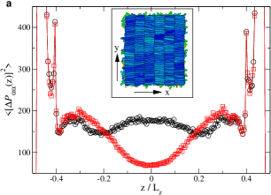
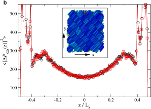
Figure 4: Tangential pressure fluctuations. Dependence of the pressure tensor fluctuations $\langle[\Delta\mathcal{P}_{xx}(z)]^{2}\rangle$ (black) and $\langle[\Delta\mathcal{P}_{yy}(z)]^{2}\rangle$ (red) on position along the $z$-axis for NEQ simulations at $P=3.6$, $T=4.0$ and $\tau=3\times 10^{4}$ for a SD configuration with the layer-normal parallel to the $x$-axis (a), and at $45^{\circ}$ with the $x$-axis (b). Insets show the top view of the cross sections of the two systems with the SD corresponding to the tangential pressure fluctuations calculated here.

Because the SD is a NESS we assume that mechanical stability is locally valid in the central part of the fluid, sufficiently removed from the walls. Locally then,

$$\nabla\cdot\boldsymbol{\mathcal{P}}={\bf 0}.$$ (4)

In equilibrium, from equation (4) follows that $\mathcal{P}_{zz}(z)=const.$ in the entire fluid. From the fact that $\langle[\Delta\mathcal{P}_{zz}(z)]^{2}\rangle$ does not depend on $z$ in the central portion of the fluid (where the SD forms, see Fig. 3) we are led to assume that a similar relation to equation (4) is valid for the pressure fluctuations

$$\nabla\cdot(\Delta\boldsymbol{\mathcal{P}})={\bf 0}.$$ (5)

Similar to standard hydrodynamics, we can then define a “fluctuation-vorticity” tensor associated to the pressure fluctuations, $\boldsymbol{\omega}\equiv\nabla\times\Delta\boldsymbol{\mathcal{P}}$. Because of the planar geometry of our system the pressure tensor components are only functions of $z$, such that $\omega_{xx}=-\partial(\Delta\mathcal{P}_{yy})/\partial z$ and $\omega_{yy}=\partial(\Delta\mathcal{P}_{xx})/\partial z$. A larger slope of $\Delta\mathcal{P}_{xx}$ or $\Delta\mathcal{P}_{yy}$ then implies a larger $\omega_{yy}$ or $\omega_{xx}$, respectively. To test whether $\boldsymbol{\omega}$ has physical significance we consider two systems with the same normal pressure fluctuations, i.e. the same $\tau$, but with different smectic-layer normals. Figure 4a shows the pressure-fluctuation profile $\langle[\Delta\mathcal{P}_{\alpha\alpha}(z)]^{2}\rangle$, $\alpha=x,y$, for a system exhibiting a SD with a smectic-layer normal parallel to the $x$-axis. The SD extends in the region $|z|/L_{z}\lesssim 0.2$. In the same region $\Delta\mathcal{P}_{xx}$ has zero slope, while $\Delta\mathcal{P}_{yy}$ exhibits a large slope. This, in turn, implies a vanishing $\omega_{yy}$ and a large $\omega_{xx}$. The relative magnitude of $\omega_{xx}$ and $\omega_{yy}$ correlates with the orientation of the smectic-layer normal. Further, in Fig. 4b we show the pressure fluctuation profile for the second SD whose smectic-layer normal is at an angle of $45^{\circ}$ with the $x$-axis. The two curves coincide (within numerical accuracy) indicating equal tangential components of $\boldsymbol{\omega}$. Therefore, from Fig. 4 we conclude that the fluctuation-vorticity $\boldsymbol{\omega}$ determines the symmetry breaking direction of alignment of the SD.

To conclude, we find evidence from NEQ computer simulations that pressure fluctuations can be easily tuned to drive a fluid system to a far-from-equilibrium state. The role of current fluctuations has been recognized zia ; hurtado_pnas11 as a stochastic variable characterizing NESS. Here, the physical picture emerging is that fluctuations in the momentum current (i) determine the NESS, and (ii) give rise to a secondary field that breaks the rotational symmetry in the $xy$-plane.

Self-assembly of molecules or supramolecular particles into layers, membranes, and vesicles is revolutionizing our control of matter across multiple length scales with far-reaching applications in nanofluidic devices brake ; woltman ; abbott11 . Chemico-physical properties are carefully tuned to obtain the desired features Genzer08 . However, in most cases they do not have any temporal dependence. The richness of NEQ phenomena in simple systems may suggest that combining the powerful new techniques of nanoscopic control with the application of time dependent external fields (temperature, electric or magnetic field, pressure and pH) may usher new ways to induce molecular self-assembly and even to simplify known tasks. In particular, the vorticity field may be used in the future to control the orientation of the ordered smectic domains which could be useful to manufacture new nanoscopic materials with distinct materials properties.

I Methods

The fluid-substrate interaction is modeled with an “integrated” Lennard-Jones potential

$$U_{fs}=4\epsilon_{fs}\rho_{\rm s}\left[\left(\frac{\sigma}{d^{\rm m}_{ik}}\right)^{10}-\left(\frac{\sigma}{d^{\rm m}_{ik}}\right)^{4}g(\hat{\mathbf{u}},t)\right]$$ (6)

where $\epsilon_{fs}=1$ and $\rho_{\rm s}\sigma^{2}=2^{2/3}\pi$ is the areal density of a single layer of atoms arranged according to the ($100$) plane of a face-centered cubic lattice. The diameter $\sigma$ of the substrate atoms is equal to the LC molecular diameter. The quantity $d^{\rm m}_{ik}$ is the minimum distance vega94 between a LC molecule and the substrate located at $z=-L_{\rm z}/2$ ($k=1$) and $z=+L_{\rm z}/2$ ($k=2$). The time-dependent anchoring $g(\hat{\mathbf{u}},t)$ is included in the attractive part of the fluid-substrate interaction. Dimensionless units are used throughout, that is, length is expressed in units of $\sigma$, temperature in units of $\epsilon_{\mathrm{ff}}/k_{\mathrm{B}}$, time in units of $(\sigma^{2}m/\epsilon_{\mathrm{ff}})^{1/2}$ using $m=1$, and pressure $P$ in units of $\sigma^{3}/\epsilon_{\mathrm{ff}}$, where $\epsilon_{\mathrm{ff}}$ is the fluid-fluid interaction energy scale of the GBK model martinez05 .

We use a velocity-Verlet algorithm for linear molecules ilnytskyi02 , and the simulations are carried out in the NPT ensemble using a Nosé-Hoover thermostat nose ; hoover and an anisotropic Hoover barostat ilnytskyi07 , whereby $L_{z}$ is kept fixed, while $L_{x}$ and $L_{y}$ are allowed to vary independently from each other, resulting in equal lateral average values of the pressure tensor $\langle\mathcal{P}_{xx}\rangle=\langle\mathcal{P}_{yy}\rangle$.

We use the “method of planes” todd to compute the component $\mathcal{P}_{zz}$ of the pressure tensor. Unfortunately, this method cannot provide $\mathcal{P}_{xx}$ and $\mathcal{P}_{yy}$ by construction, which instead we compute following Harasima’s method harasima .

References

- (1) F. Ritort, Adv. Chem. Phys. 137, 31 (2008).
- (2) M. C. Cross and P. C. Hohenberg, Rev. Mod. Phys. 65, 851 (1993).
- (3) C. Van den Broeck, J. M. R. Parrondo, and R. Toral, Phys. Rev. Lett. 73, 3395 (1994).
- (4) V. Schaller, C. Weber, C. Semmrich, E. Frey, and A. R. Bausch, Nature 467, 73 (2010).
- (5) P. Kraikivski, R. Lipowsky, and J. Kierfeld, Phys. Rev. Lett. 96, 258103 (2006).
- (6) V. Narayan, S. Ramaswamy, and N. Menon, Science 317, 105 (2007).
- (7) F. Jülicher, A. Ajdari, and J. Prost, Rev. Mod. Phys. 69, 1269 (1997).
- (8) Z. Rácz, in Slow Relaxations and nonequilibrium dynamics in condensed matter, edited by J.-L. Barrat, M. V. Feigelman, J. Kurchan, and J. Dalibard (Springer-Verlag, Berlin, Heidelberg, 2002).
- (9) U. Seifert, Eur. Phys. J. B 64, 423 (2008).
- (10) D. J. Evans, E. G. D. Cohen, and G. P. Morriss, Phys. Rev. Lett. 71, 2401 (1993).
- (11) G. Gallavotti and E. G. D. Cohen, Phys. Rev. Lett. 74, 2694 (1995).
- (12) C. Jarzynski, Phys. Rev. Lett. 78, 2690 (1997).
- (13) U. Seifert, Phys. Rev. Lett. 95, 040602 (2005).
- (14) T. Schmiedl, T. Speck, and U. Seifert, J. Stat. Phys. 128, 77 (2007).
- (15) R. K. P. Zia and B. Schmittmann, J. Stat. Mech. 2007, P07012 (2007).
- (16) P. I. Hurtado and P. L. Garrido, Phys. Rev. E 81, 041102 (2010).
- (17) P. I. Hurtado, C. Pérez-Espigares, J. J. del Pozo, and P. L. Garrido, Proc. Nat. Acad. Sci. USA 108, 7704 (2011).
- (18) L. Bertini, A. D. Sole, D. Gabrielli, G. Jona-Lasinio, and C. Landim, J. Stat. Mech. P07014 (2007).
- (19) B. Derrida, J. Stat. Mech. P07023 (2007).
- (20) B. Martínez-Haya, A.Cuetos, S. Lago, and L. F. Rull, J. Chem. Phys. 122, 024908 (2005).
- (21) A. A. Sonin, The surface physics of liquid crystals (Gordon and Breach, Amsterdam, 1995).
- (22) Y. Bai and N. L. Abbott, Langmuir 27, 5719 (2011).
- (23) M. A. C. Stuart, W. T. S. Huck, J. Genzer, M. Müller, C. Ober, M. Stamm, G. B. Sukhorukov, I. Szleifer, V. V. Tsukruk, M. Urban, F. Winnik, S. Zauscher, I. Luzinov, and S. Minko, Nature Materials 9, 101 (2010).
- (24) B. H. Clare, K. Efimenko, D. A. Fischer, J. Genzer, and N. L. Abbott, Chemistry of Materials 18, 2357 (2006).
- (25) L. Ionov, N. Houbenov, A. Sidorenko, M. Stamm, I. Luzinov, and S. Minko, Langmuir 20, 9916 (2004).
- (26) J. R. Matthews, D. Tuncel, R. M. J. Jacobs, C. D. Bain, and H. L. Anderson, Journal of the American Chemical Society 125, 6428 (2003).
- (27) J. Song and G. J. Vancso, Langmuir 27, 6822 (2011).
- (28) C. L. Feng, Y. J. Zhang, J. Jin, Y. L. Song, L. Y. Xie, G. R. Qu, L. Jiang, and D. B. Zhu, Langmuir 17, 4593 (2001).
- (29) N. G. van Kampen, Stochastic processes in physics and chemistry (North Holland, Amsterdam, 2002).
- (30) J. M. Brake, M. K. Daschner, Y.-Y. Luk, and N. L. Abbott, Science 302, 2094 (2003).
- (31) S. J. Woltman, G. D. Jay, and G. P. Crawford, Nature Materials 6, 929 (2007).
- (32) J. Genzer and R. R. Bhat, Langmuir 24, 2294 (2008).
- (33) C. Vega and S. Lago, Comput. Chem. 18, 55 (1994).
- (34) J. M. Ilnytskyi and M. R. Wilson, Comput. Phys. Commun. 148, 43 (2002).
- (35) S. Nosé, J. Chem. Phys. 81, 511 (1984).
- (36) W. G. Hoover, Phys. Rev. A 31, 1695 (1985).
- (37) J. M. Ilnytskyi and D. Neher, J. Chem. Phys. 126, 174905 (2007).
- (38) B. D. Todd, D. J. Evans, and P. J. Daivis, Phys. Rev. E 52, 1627 (1995).
- (39) A. Harasima, Adv. Chem. Phys. 1, 203 (1958).