Preparing and Probing Atomic Majorana Fermions and Topological Order in Optical Lattices

Abstract

We introduce a one-dimensional system of fermionic atoms in an optical lattice whose phase diagram includes topological states of different symmetry classes with a simple possibility to switch between them. The states and topological phase transitions between them can be identified by looking at their zero-energy edge modes which are Majorana fermions. We propose several universal methods of detecting the Majorana edge states, based on their genuine features: zero-energy, localized character of the wave functions, and induced non-local fermionic correlations.

1 Introduction

There is at present growing interest in topological phases of matter – fermionic insulators and superconductors with a gapped excitation spectrum and nonlocal topological order (TO). TO is characterized by a topological invariant taking discrete values [1, 2, 3, 4, 5, 6]. An immediate consequence of TO is the existence of robust zero-energy modes localized at defects, edges, and interfaces between different topological phases [7, 8, 9]. The number of these states and their properties are directly linked to TO and, therefore, can be viewed as a probe of the topological state providing access to the corresponding phase diagram. A striking example are zero-energy Majorana fermions, as discussed in the context of topological quantum computing [10, 11, 12].

Most of the developments and proposals to realize and study topological phases in general, and Majorana fermions in particular, have been related to condensed matter systems [13, 14, 15, 16, 17], with a first observation of Majorana edge modes in a hybrid superconductor-semiconductor nanowire device recently reported in Ref. [18]. On the other hand, there are several promising proposals to realize topological phases with quantum degenerate gases of atoms and molecules [19, 20, 21, 22, 23, 24], with questions of detection of such phases presently in the focus of interest [25, 29, 30, 31]. Below we will outline a measurement scenario for topological phases and phase transitions by monitoring signatures of Majorana fermion edge-states in atomic systems. Our analysis builds directly on recent experimental advances such as single site addressing and measurements in optical lattices [26, 27] in combination with traditional time of flight and spectroscopic techniques, and complements the recent proposals to detect topology in the bulk as proposed in [29, 30, 31].

To illustrate our ideas for detection we introduce a simple, but experimentally realistic example of a zig-zag chain (c.f. Fig. 1a). This model is an extension of the familiar Kitaev model of spin-less fermions coupled to a BCS-reservoir with the additional feature of next-to-nearest neighbor couplings (see below), and can be realized with cold atoms generalizing ideas outlined in Ref. [23]. The model has a remarkably rich phase diagram, allowing different topological states in two symmetry classes supporting Majorana edge modes, and provides an ideal playground to demonstrate the presence of TO and the topological phase transitions via related Majorana edge states. We propose a fully reproducible preparation of an initial state for Majorana fermions and detection with atomic measurement techniques, including (i) zero-energy, (ii) localization near the edge and (iii) induced non-local fermionic correlations, which, together, allow for an unambiguous probe of Majorana fermions. While the present example is 1D, the techniques described below have a straightforward extension to 2D, as illustrated by discussion of a $p_{x}+ip_{y}$ superfluid.

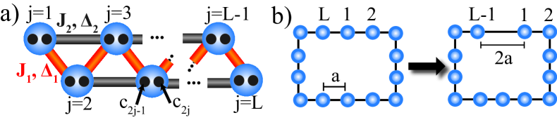
Figure 1: a) A zig-zag chain of spinless fermionic atoms according to the Hamiltonian $H$ with NN (red) and NNN couplings (grey). $c_{2j-1}$ and $c_{2j}$ denote Majorana operators on lattice sites $j=1$ to $L$ (see text). b) Preparation of the initial state of Majorana fermions by adiabatically cutting the closed chain.

2 The Zig-zag Chain

In the following Section we discuss the Zig-zag Chain, a one-dimensional ($1D$) model system of spinless fermions which allows for a variety of topological phases, thus providing an ideal playground for testing our detection techniques. We start in Subsec. 2.1 introducing the model and presenting its topological phase diagram. The reader interested in the derivation of these results is referred to Subsec. 2.2 . Further, we review the ideas of  [23] in Subsec. 2.3, explaining how the zig-zag chain can be realized in a cold atom implementation.

2.1 The Model System and its Properties

We consider single-component fermions on a finite $1D$ chain of size $L$ with Hamiltonian $H=H_{1}+H_{2}+H_{\mu}$ (c.f. Fig. 1a). Here, $H_{\mu}=-\mu\sum_{j=1}^{L}a_{j}^{\dagger}a_{j}$, and

$$H_{\alpha}=\sum_{j=1}^{L-\alpha}\left[-J_{\alpha}a_{j}^{\dagger}a_{j+\alpha}+\Delta_{\alpha}a_{j}a_{j+\alpha}+h.c.\right].$$ (1)

where $a_{i}$ and $a_{i}^{\dagger}$ are fermionic operators ($i=1,\ldots,L$), $J_{\alpha}\geq 0$ and $\Delta_{\alpha}=\left|\Delta_{\alpha}\right|e^{i\phi_{\alpha}}$ are nearest-neigbour (NN, $\alpha=1$) and next-to-nearest-neighbour (NNN, $\alpha=2$) hopping and pairing amplitudes, respectively, and $\mu$ is the chemical potential. As shown in  [23] and reviewed in Subsec. 2.3, the pairing terms in $H_{\alpha}$ are obtained by a Raman induced dissociation of Cooper pairs (or Feshbach molecules) forming an atomic BCS reservoir, with $\mu$ a Raman detuning. In Fig. 1a we represent the chain as a zig-zag, which leads naturally to a cold atom implementation with optical lattices allowing control of the relative strength of NN and NNN amplitudes by changing the zig-zag geometry.

Although $H$ can be viewed as a Hamiltonian of two coupled Kitaev chains [32] (with odd or even sites), the resulting topological phase diagram is substantially richer. Since the coupling parameters can be changed in a real-time experiment, this setup gives rise to a platform for exploring topological properties of matter, including topological phase transitions and Majorana fermions. We summarize here only the main features of the topological phase diagram, and refer the interested reader to Subsec. 2.2

The topological symmetry class [1] of $H$ depends crucially on the relative phase $\phi=\phi_{1}-\phi_{2}$ of the pairing amplitudes (one of the phases, say, $\phi_{2}$, can be gauged away by redefining the operators $a_{j}$). For $\phi=0,\pi$ $(\mathrm{mod}\,2\pi)$ it is the class BDI (Cartan) with time-reversal, particle-hole, and chiral symmetries, for all other values of $\phi$ it is class D with only particle-hole symmetry. Both classes allow topologically nontrivial states characterized by the integer-valued winding number $\nu\in\mathbb{Z}$ in the class BDI and by the Chern parity number $P_{C}=0,1\in\mathbb{Z}_{2}$ in the class D.

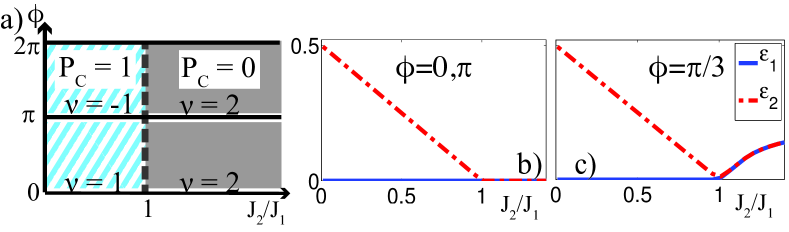
Figure 2: a) Phase diagram corresponding to the Hamiltonian $H$ for $\mu=0$, $|\Delta_{\alpha}|=J_{\alpha}e^{i\phi}$. b) The two lowest doubly degenerate eigenvalues $\varepsilon_{1,2}$ of $H$ as a function of the ratio $J_{2}/J_{1}$: If $\phi=0,\pi$ $(\mathrm{mod}\,2\pi)$ (BDI class) there are one or two such modes (b), for all other values of $\phi$ (D class), there is at most one zero mode (c) (see also Subsec. 2.2).

The topological phase diagram contains states with $\nu=0,\pm 1,\pm 2$ for the BDI class, and with $P_{C}=0,1$ for the D class. Fig. 2a summarizes results for the simplest case $\mu=0$ and $\left|\Delta_{\alpha}\right|=J_{\alpha}$, where the phase diagram is characterized by the relative phase $\phi$ and the ratio $J_{2}/J_{1}$. We find that $\nu=2,P_{C}=0$ for $J_{2}>J_{1}$, else one has $P_{C}=1$ and $\nu=+1$ or $-1$ for $\phi=0$ and $\pi$, respectively. Therefore, for both symmetry classes, the point $J_{1}=J_{2}$ corresponds to a topological phase transition, where the bulk excitations become gapless (see Subsec. 2.2).

The presence of a nontrivial TO in the bulk leads to zero-energy modes, which in our case are Majorana fermions, at the interfaces between states with different TO. The number of these states is related to the difference of the corresponding topological invariants [8, 9]. Using the hermitian Majorana representation, where $c_{2j-1}=a_{j}^{\dagger}+a_{j}$ and $c_{2j}=(-i)(a_{j}^{\dagger}-a_{j})$ obey $\{c_{j},c_{l}\}=2\delta_{jl}$, the quadratic Hamiltonian reads $H=i\sum_{j,l}A_{jl}c_{j}c_{l}$ with real $A=-A^{T}$. Diagonalizing $A$ for a finite chain we identify the zero-energy modes and associated Majorana edge-mode operator $\gamma_{E}=\sum_{k}v_{Ek}c_{k}$ with (real) coefficients $v_{Ek}$ localized at the interface with some localization length $l_{\mathrm{loc}}$. [To be precise, the energy of these modes $\sim\exp(-L/l_{\mathrm{loc}})$ approaches zero for $L\rightarrow\infty$.] Thus, by detecting Majorana zero-energy edge modes and their number we can access the full topological phase diagram of our model:

For the BDI class we have in total two such modes for $J_{1}>J_{2}$: $\gamma_{L}=c_{1}$ and $\gamma_{R}=c_{2L}$ for the left and the right edge, respectively, and four modes for $J_{1}<J_{2}$. The two additional zero modes are exponentially decaying inside the bulk (see Fig. 2b and Subsec. 2.2). For the D class there are two zero-energy modes for $J_{1}>J_{2}$, which decay exponentially inside the chain, and no such modes for $J_{1}<J_{2}$ (Fig. 2c).

The presence of Majorana zero-energy modes comes along with a degeneracy of the ground state: The dimension of the ground-state subspace is $2^{N_{M}/2}$, where $N_{M}$ is the number of the Majorana modes (always even in our case). A state in this subspace generically has correlations between Majorana operators from different edges, resulting in non-local fermionic correlations (in contrast to local correlations in the bulk). For the case with only two Majorana modes ($\nu=1$ or $P_{C}=1$), the two ground states $\left|G_{\pm}\right\rangle$ have even ($+$) or odd ($-$) number of fermions, respectively, and the nonlocal correlations $\left\langle G_{\pm}\right|\gamma_{L}\gamma_{R}\left|G_{\pm}\right\rangle=\pm i$ are related to the fermionic parity, in full analogy to Ref. [32].

2.2 Derivation of the Topological Phase Diagram

In the following we present a detailed derivation of the topological phase diagram presented in Subsec. 2.1. According to the general tenfold classification scheme [1, 3], the topological class to which a given Hamiltonian belongs to, is determined by the invariance properties of the Hamiltonian under time-reversal, particle-hole (or charge conjugation), and chiral (or sublattice) symmetry. This class specifies then, whether the states with a nontrivial topological order could exist and provides the corresponding topological invariant to distinguish them.

For a translationally invariant $1D$ spinless Bogoliubov-de Gennes lattice Hamiltonian in the quasimomentum basis

$$H=\sum_{k\in\mathrm{BZ}}\Psi_{k}^{\dagger}\mathcal{H}_{k}\Psi_{k},$$ (2)

where

$$\mathcal{H}_{k}=\left(\begin{array}[]{cc}\xi_{k}&\Delta_{k}\\ \Delta_{k}^{\ast}&-\xi_{k}\end{array}\right),\quad\Psi_{k}=\left(\begin{array}[]{c}a_{k}\\ a_{-k}^{\dagger},\end{array}\right)$$ (3)

with $a_{k}=L^{-1/2}\sum_{k}e^{ikj}a_{j}$, the invariances are equivalent to the following conditions:

$$U_{T}^{\dagger}\mathcal{H}_{k}U_{T}=\mathcal{H}_{-k}^{\ast},$$

for the time-reversal,

$$U_{C}^{\dagger}\mathcal{H}_{k}U_{C}=-\mathcal{H}_{-k}^{\ast},$$

for the particle-hole, and

$$\Sigma^{\dagger}\mathcal{H}_{k}\Sigma=-\mathcal{H}_{k},$$

for the chiral symmetries, respectively, where $U_{T}$, $U_{C}$, and $\Sigma$ are unitary matrices satisfying $U_{T}U_{T}^{\ast}=\pm 1$, $U_{C}U_{C}^{\ast}=\pm 1$, and $\Sigma^{2}=1$.

For the Hamiltonian $H$ of Eq. (1) one has $\xi_{k}=-(J_{1}\cos k+J_{2}\cos 2k)-\mu/2$ and $\Delta_{k}=-i(\Delta_{1}\sin k+\Delta_{2}\sin 2k)$, such that the matrix $\mathcal{H}_{k}$ is

$$\mathcal{H}_{k}=\vec{h}_{k}\cdot\vec{\sigma},$$

where $\vec{\sigma}=\{\sigma_{x},\sigma_{y},\sigma_{z}\}$ is the vector of Pauli matrices and $\vec{h}_{k}^{T}=[\mathrm{Re},-\mathrm{Im}(\Delta_{k})(\Delta_{k}),\xi_{k}]$. The excitation energies are $E_{k}=2\left|\vec{h}_{k}\right|=2\sqrt{\xi_{k}^{2}+\left|\Delta_{k}\right|^{2}}$.

For generic $\Delta_{1}=\left|\Delta_{1}\right|e^{i\phi_{1}}$ and $\Delta_{2}=\left|\Delta_{2}\right|e^{i\phi_{2}}$, only the particle-hole symmetry condition is fulfilled with $U_{C}=\sigma_{x}$ (as it should be for a general Bogoliubov-de Gennes Hamiltonian), and, therefore, the Hamiltonian $H$ belongs to the class D. For $\phi\equiv\phi_{1}-\phi_{2}=0$ or $\pi$ $\mathrm{mod}2\pi)$, that is $\Delta_{k}=-ie^{i\phi_{2}}(\varepsilon\left|\Delta_{1}\right|\sin k+\left|\Delta_{2}\right|\sin 2k)$ with $\varepsilon=\exp(i\phi)=\pm 1$, the conditions for the time-reversal and chiral symmetries are also satisfied with $U_{T}=\mathrm{diag}(e^{-i\phi_{2}},e^{i\phi_{2}})$ and $\Sigma=\sigma_{x}U_{T}$, and the Hamiltonian $H$ belongs to the chiral BDI class. Note that the phase $\phi_{2}$ can be gauged away by $a_{k}\rightarrow e^{-i\phi_{2}/2}a_{k}$ such that $\mathrm{Re}(\Delta_{k})=0$ and the vector $\vec{h}_{k}$ belongs to the $yz$-plane for all $k$. Geometrically speaking, for the BDI class the vectors $\vec{h}_{k}$ for all $k$ are in the same plane, which is the $yz$-plane for $\phi_{2}=0$.

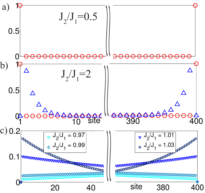
Figure 3: Spatial distribution of the zero energy modes of $H$ for $J_{\alpha}=|\Delta_{\alpha}|$ and $\phi=0$. a) If $J_{2}<J_{1}$ we have two zero energy modes that are located at the boundary. b) If $J_{2}>J_{1}$, two additional zero energy modes with an exponential decay appear. c) These modes extend more and more over the lattice when we approach the transition point $J_{2}=J_{1}$.

For the chiral BDI class in $1D$, different topological states are classified by the integer valued winding number $\nu\in\mathbb{Z}$ defined in the following way (see, for example, [7]): By gauging away the phase $\phi_{2}$ and using a unitary transformation $U=\exp(i\pi\sigma_{y}/4)$, the Hamiltonian can be transformed into a canonical form

$$\mathcal{H}_{k}=\left(\begin{array}[]{cc}0&q_{k}\\ q_{k}^{\ast}&0\end{array}\right)=\left|q_{k}\right|\left(\begin{array}[]{cc}0&e^{i\varphi_{q_{k}}}\\ e^{-i\varphi_{q_{k}}}&0\end{array}\,\right)$$ (4)

with $q_{k}=$ $\xi_{k}+\Delta_{k}$ and $\varphi_{q_{k}}$ being the phase of $q_{k}$. Then

$$\nu=\frac{1}{2\pi}\int_{-\pi}^{\pi}dk\frac{d\varphi_{q_{k}}}{dk}=\varphi_{q_{k=\pi}}-\varphi_{q_{k=-\pi}}\in\mathbb{Z}$$

Alternatively, the winding number can be defined using the unit vector $\vec{n}_{k}=\vec{h}_{k}/\left|\vec{h}_{k}\right|$ in the $yz$-plane ($\phi_{2}$ is gauged away)

$$\nu=\frac{1}{2\pi}\int_{-\pi}^{\pi}\hat{e}_{x}\cdot(\vec{n}_{k}\times\partial_{k}\vec{n}_{k})dk\in\mathbb{Z},\;$$

as number of times the vector $\vec{n}_{k}$ wraps around the unit circle when $k$ goes around the Brioullin zone (here $\hat{e}_{x}$ is the unit vector along the $x$-axis). Note that as long as $\left|\vec{h}_{k}\right|\neq 0$ (or, equivalently, $\left|q_{k}\right|\neq 0$), which corresponds to the gapped spectrum of the Hamiltonian, the winding number is well-defined and, therefore, can change its value only when the gap closes. This gap-closing condition is the necessary one for the topological phase transition.

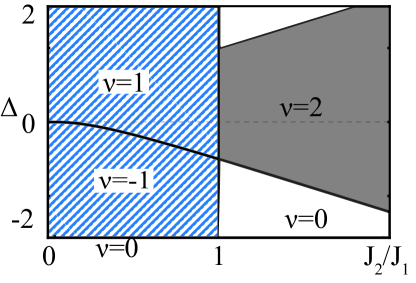
Figure 4: Topological phase diagram in the chiral class for the case $\left|\Delta_{1}\right|\neq J_{1}$ but still $\Delta_{2}=J_{2}$ and $\mu=0$. We see that we can obtain regions with $\nu=0$ (white), $1$ (striped) and $2$ (grey).

For $\left|\Delta_{\alpha}\right|=J_{\alpha}$ and $\mu=0$, the gap closing condition corresponds to $J_{1}=J_{2}$, and straightforward calculations give $\nu_{\phi=0}=\frac{1}{2}\left[3-\mathrm{sign}\left(\frac{J_{1}-J_{2}}{J_{1}+J_{2}}\right)\right]$ and $\nu_{\phi=\pi}=\frac{1}{2}\left[1-3\mathrm{sign}\left(\frac{J_{1}-J_{2}}{J_{1}+J_{2}}\right)\right]$. For $J_{1}=J_{2}$ we indeed have a topological phase transition between two different states. For a finite chain, the winding number manifests itself in the number of zero-energy modes localized near the chain edges, see Figs. 3a and 3b. When one approaches the topological phase transition point, say, from the side $J_{2}>J_{1}$, two out of four zero-energy modes start to proliferate inside the bulk of the chain and become gapped on the other side of the transition; see Fig. 3c.

The topological phase diagram in this chiral class for the case $\left|\Delta_{1}\right|\neq J_{1}$, but still $\Delta_{2}=J_{2}$ and $\mu=0$, is shown in Fig. 4. In this case $\vec{h}_{k}=(0,\Delta_{1}\sin k+J_{2}\sin 2k,J_{1}\cos k+J_{2}\cos 2k)$, where we assume $\phi_{2}=0$, and, hence, real $\Delta_{1}$. The boundaries between different topological phases results from the condition $\left|\vec{h}_{k}\right|=0$.

For the D class [when $\phi\neq 0,\pi(\mathrm{mod}2\pi)$], there are only two different classes of the topological states characterized by the Chern parity number $P_{C}\in\mathbb{Z}_{2}$. To define this topological invariant [4], one has to extend the Hamiltonian $\mathcal{H}_{k}$ and thus $\vec{h}_{k}$ from a one-dimensional Brillouin zone $k\in[-\pi,\pi]\sim S^{1}$ (topologically equivalent to the circle $S^{1}$) to a two-dimensional ($2D$) Brillouin zone $k,t\in[-\pi,\pi]\sim S^{1}\times S^{1}=T^{2}$ (topologically equivalent to a two-dimensional torus $T^{2}$), $\mathcal{H}_{k}\rightarrow\mathcal{H}_{k,t}=$ $\vec{h}_{k,t}\cdot\vec{\sigma}$, such that the resulting Hamiltonian is gapped and belongs to the D class in $2D$: $\sigma_{x}\mathcal{H}_{-k,-t}^{\ast}\sigma_{x}=-\mathcal{H}_{k,t}$ . The unit vector $\vec{n}_{k,t}=\vec{h}_{k,t}/|\vec{h}_{k,t}|$ maps then the $2D$ Brillouin zone $T^{2}$ into a $2D$ sphere $S^{2}$. Different topological classes of such mappings are distinguished by the integer-valued Chern number

$$C=\int_{-\pi}^{\pi}\frac{dkdt}{4\pi}\vec{n}_{k,t}\cdot(\partial_{k}\vec{n}_{k,t}\times\partial_{t}\vec{n}_{k,t})\in\mathbb{Z}.$$

It turns out [4], that the parity $P_{C}$ of $C$ does not depend on the chosen extension of the Hamiltonian, and, therefore, provides the topological invariant for $1D$ Hamiltonians in the D class. (We set $P_{C}=1$ for odd $C$ and $P_{C}=0$ for even $C$. Topologically nontrivial states correspond to $P_{C}=1$.)

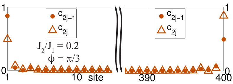
Figure 5: Spatial distribution of the zero modes for $\phi=\pi/3$ and $J_{2}/J_{1}=0.2$. There are two zero modes (left and right) which are linear combinations of only even or only odd Majorana operators living on a site $j$.

The extension can be constructed using a hermitian matrix $\bar{\mathfrak{h}}(k,t)=\sum_{i}\mathfrak{h}_{i}(k,t)\sigma_{i}$, which has a gapped spectrum and depends on two parameters $k\in[-\pi,\pi]$ and $t\in[0,\pi]$ such that $\bar{\mathfrak{h}}(k,0)=\mathcal{H}_{k}$ and $\bar{\mathfrak{h}}(k,\pi)=|\vec{h}_{k}|\sigma_{z}$. Note that $\bar{\mathfrak{h}}(k,t)$ interpolates between the initial Hamiltonian $\mathcal{H}_{k}$ and the ”trivial” one $|\vec{h}_{k}|\sigma_{z}$, both from the D class (for $t\neq 0$ or $\pi$, $\bar{\mathfrak{h}}(k,t)$ does not necessarily belong to the D class in $1D$). Such a matrix always exists because it belongs to the A class of general hermitian matrices (with no symmetries) with a gapped spectrum that is topologically trivial. Then the matrix

$$\mathcal{H}_{k,t}=\cases{\bar{\mathfrak{h}}(k,\pi+t),&for\; $t\in[-\pi,0]$\\ -\sigma_{1}\bar{\mathfrak{h}}^{T}(-k,\pi-t)\sigma_{1}&for $t\in[0,\pi]$\\ }$$ (5)

is in the D class and provides the desired extension. The interpolation $\bar{\mathfrak{h}}(k,t)$ can be obtained, for example, in the following way: $\mathfrak{h}_{i}(k,t)$ for $t\in[0,\pi/2]$ corresponds to a rotation of $\vec{h}_{k}=\mathfrak{h}_{i}(k,0)$ to the $y$-axes, such that $\mathfrak{h}_{i}(k,\pi/2)$ is parallel to the $y$-axes for all $k$, and then $\bar{\mathfrak{h}}(k,t)$ for $t\in[\pi/2,\pi]$ describes the rotation of $\mathfrak{h}_{i}(k,\pi/2)$ to the $z$-axis.

Following this strategy for the case $\left|\Delta_{\alpha}\right|=J_{\alpha}$ with $\mu=0$ we find $C=0$ for $J_{2}>J_{1}$ and $C=\mathrm{sign}(\sin\phi)$ for $J_{1}>J_{2}$, where $\phi=\phi_{1}-\phi_{2}$. The point $J_{1}=J_{2}$ corresponds to the topological phase transition, at which the gap vanishes, see Fig. 2c.

2.3 AMO realization of the Zig-zag Chain

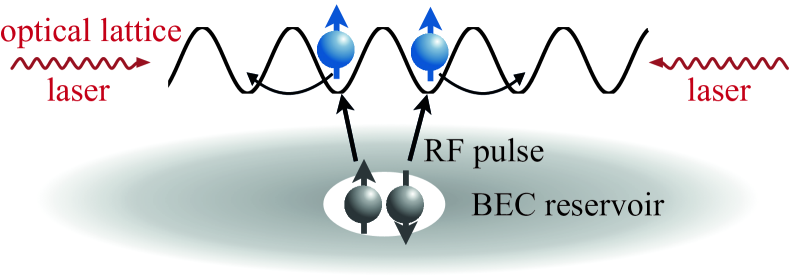
Figure 6: Creation of the pairing term $\Delta a^{\dagger}_{j}a^{\dagger}_{j+1}+h.c.$ according to Ref [23]. A one-dimensional system of trapped fermions in two spin states is coupled to a molecular BEC via a RF pulse. An additional Raman laser with strong driving projects out one of the spin components, leading to the desired pairing term.

The zig-zag chain defined in Eq. (1) allows for an optical lattice realization, as we briefly explain in this Subsection (see also Fig. 6). While the hopping term $a^{\dagger}_{j}a_{j+\alpha}+h.c.$ arises naturally in an optical lattice setup, the pairing term $a^{\dagger}_{j}a^{\dagger}_{j+\alpha}+h.c.$ can be engineered via the coupling of the system to a BEC reservoir of Feshbach molecules, as explained in [23]. The main idea is to couple the two internal spin states of the trapped $1D$ system of fermions to a Feshbach molecule via an RF pulse. If we denote by $(a^{\dagger}_{p,\uparrow},a^{\dagger}_{p,\downarrow})$ the two internal states of the trapped atoms with momentum $p$, then the result of the RF pulse is an effective pairing term of the form $\Delta a^{\dagger}_{p,\uparrow}a^{\dagger}_{-p,\downarrow}+h.c$. Driving the lattice fermions additionally with a Raman laser creates an effective magnetic field, which for strong driving (i.e. large magnetic fields) projects out one of the spin components, such that we obtain the spinless pairing term of Eq. (1)  [23].

3 Preparation of Majorana modes

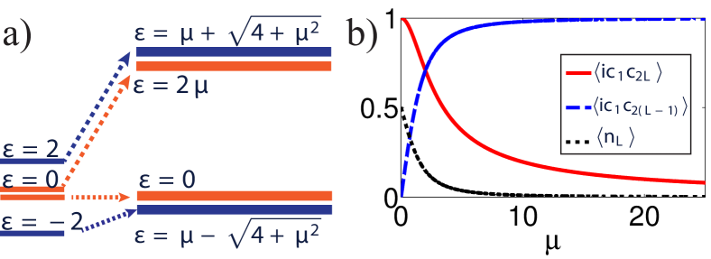
Figure 7: a)Evolution of energy spectrum of the Hamiltonian $H(\mu)=H_{K}+\mu(t)a_{L}^{\dagger}a_{L}|_{j=1,L}$ for an adiabatic ramp of $\mu$. b) Evolution of the occupation of the site $L$ and the Majorana correlation functions during the adiabatic ramp.

The main difficulty in detecting the Majorana modes is that their signal comes only from the edges and, therefore, has poor signal-to-noise ratio. To overcome this, an experiment has to be performed several times thus requiring a reproducible preparation of a desired initial quantum state of an open wire. In our setup, this can be achieved by starting with a closed quantum chain in a fully paired [34, 35] (and, hence, unique) state corresponding to the ground state of a Hamiltonian (see Fig. 1b)). This state has an even parity (all particles are paired) and only local correlations between the sites. Making use of local addressing [26, 27] we can ”cut” the chain by ramping up the chemical potential on the site $L$,

$$H(\mu)=H+\mu(t)a_{L}^{\dagger}a_{L}.$$

This process affects only the four Majorana modes $c_{2L-2},c_{2L-1},c_{2L},c_{1}$, and the corresponding instantaneous eigenvalues are $0$ and $2\mu$ for the odd parity sector, and $\mu\pm\sqrt{4+\mu^{2}}$ for the even one, such that there are two degenerate ground states of the Kitaev chain for $\mu\rightarrow\infty$. Because a superposition of fermionic states with different parity is forbidden by superselection rules, the corresponding eigenstates never mix during the adiabatic ramp (cf. Fig. 7a), and, hence, the final state of the open chain has even parity. In Fig. 7b we depict the evolution of the Majorana correlation functions between nearest- ($\langle ic_{1}c_{2L}\rangle$, solid) and next-to-nearest ($\langle ic_{1}c_{2L-1}\rangle$, dashed) neighbors, as well as the occupation of the site $L$ ($\langle n_{L}\rangle$, dotted) during the adiabatic ramp.

For the ”zig-zag” chain we can start with two decoupled closed chains (with even and odd lattice sites) when only $\Delta_{2}$ and $J_{2}$ are nonzero but $\Delta_{1}=J_{1}=0$. We then cut them as described above into two open chains each with two edge Majorana modes and in the even fermionic parity state with all fermions being paired. Now we can switch $J_{1}$ and $\Delta_{1}$ on adiabatically to create a single quantum chain with even parity. Note that during this process there is no single-particle transition between the two subchains (with even and odd sites) because such a transfer would create single-particle excitations in both subchains which cannot occur in an adiabatic process due to the conservation of energy. Thus, each of the subchains remains in the even parity state.

Further increase of NN amplitudes results in a topological phase transition with closing the single-particle excitation gap allowing for a single-particle exchange between the subchains. Then, only the (even) parity of the entire chain is preserved. We would like to add here that parity violating processes, such as three-body losses, are sufficiently weak in fermionic systems (0.1–1s) in order not to be an experimental obstacle for the realization of Majorana physics

Note that a similar idea can be used to create the initial Majorana state in the dissipative setting by adiabatically emptying one site  [24]. Note that the cutting procedure avoids the need to establish the edge-edge correlations via a sequential process, which takes polynomial time due to the Lieb-Robinson bound [36, 37].

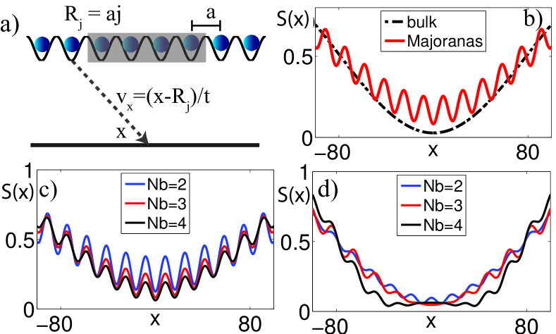
Figure 8: a) Principle of TOF. The contrast of the signal can be enhanced by excluding the bulk (grey shade). b) TOF for the ideal Kitaev chain of length $L_{M}=20$: The presence of the Majorana modes (solid) leads to oscillations of the signal $S(x)$ (see main text) which are absent in the bulk (dashed). Having their origin in nonlocal fermionic correlations of modes located at the edges, the oscillation frequency is independent of the size of the shade (c) which allows to rule out a finite size effect encountered, e.g. in a system of freely hopping particles (d) (see main text).

4 Time-of-Flight (TOF) imaging

Having prepared the atomic Majorana fermions following the protocol presented in Sec. 3, we present now two possibilities to detect them in AMO setups. The first approach that is discussed in this Section is based on Time-of-Flight imaging allows to detect the existence and number of Majorana fermions in an optical lattice setup. Further, we present a complementary approach based on a spectroscopic setup in Sec.  5.

Non-local correlations can be detected in TOF imaging, as illustrated in Fig. 8a. We consider atoms of mass $m$ released at time $t=0$ from lattice sites $R_{j}=ja$ with lattice spacing $a$. At time $t\gg ma^{2}/\hbar$ (far field approximation) the atomic density distribution at the detector is given by $\langle n(x)\rangle\sim\sum_{j,j^{\prime}}e^{2ix(R_{j}-R_{j^{\prime}})m/(\hbar t)}\langle a_{j}^{\dagger}a_{j^{\prime}}\rangle$ revealing the initial correlations of the atoms in the lattice. Therefore, the long-range Majorana correlations $R_{j}-R_{j^{\prime}}\approx L_{M}$ (distance between the edge modes) will result in rapid oscillations of $\langle n(x)\rangle$ as compared to slow oscillations originating from short-range bulk correlations ($R_{j}-R_{j^{\prime}}\approx a$). The contrast of the Majorana signal can be enhanced by local addressing: we shade all but $N_{b}$ sites adjacent to each of the two edges ($N_{b}=2$ in Fig. 8a), thus measuring $\langle n(x)\rangle=2N_{b}S(x)$, where we have normalized by the number of sites contributing to the signal, $2N_{b}$.

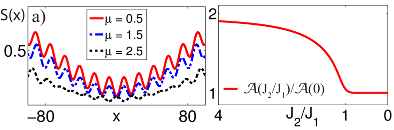
Figure 9: TOF as a method for detecting topological phase transitions: a) The TOF signal for a single wire vanishes if we approach the transition point at $\mu=2$. d) The amplitude of $S(x)$ allows to determine the number of Majorana modes in the BDI class of our model (see main text).

The calculation of the density distribution at the detector in a TOF experiment requires the knowledge of the first moments $\langle a_{j}^{\dagger}a_{j^{\prime}}\rangle$ of the state in the lattice before the trapping potential is switched off. For $J_{\alpha}=\Delta_{\alpha}$, $J_{2}=\mu=0$ (ideal Kitaev chain), the non-vanishing first moments in the Majorana language are $\langle c_{2j}c_{2k}\rangle_{\pm}=\langle c_{2j+1}c_{2k+1}\rangle_{\pm}=\delta_{kj}$, $\langle c_{2j}c_{2k+1}\rangle_{\pm}=-\langle c_{2j+1}c_{2k}\rangle_{\pm}=-i\delta_{kj}$, and the edge-edge correlations are given by $\langle c_{2L}c_{1}\rangle_{\pm}=im_{\pm}(d)$ [$m(d)=0$ if we consider the bulk only] with $d$ being the distance between the two Majorana edge modes. When only $N_{b}$ sites on the right and on the left sides of the chain contribute to the signal (other sites are covered with a shade), the atom density distribution at the detector reads

$$\langle n(x)\rangle_{+}\sim\mathcal{N}_{bulk}(x)+m(d)\mathcal{N}_{edge}(x),$$

where $\mathcal{N}_{bulk}(x)=2N_{b}\sin^{2}(\frac{mxa}{\hbar t})+\cos(\frac{mxa}{\hbar t})$ stems from the atoms in the bulk only and the two edge sites separated by $L_{M}=ad$ give rise to $\mathcal{N}_{edge}(x)=\cos(\frac{mxa}{\hbar t}d)/2$ multiplied by the Majorana correlation $m(d)=-i\left\langle\gamma_{L}\gamma_{R}\right\rangle$. For the general case, we obtain the correlation matrix $\langle a^{\dagger}_{j}a_{j^{\prime}}\rangle$ via a numerical diagonalization of the Hamiltonian $H$.

We see that the second rapidly oscillating term reflects the presence of the long-range Majorana correlations and allows to determine the occupation of the Majorana subspace. If the initial state of the chain is prepared as described above, then $m(d)=-i\left\langle G_{+}\right|\gamma_{L}\gamma_{R}\left|G_{+}\right\rangle=1$, and the amplitude of this terms reaches its maximum. The results of the calculations for the ideal chain are shown in Fig. 8b: The presence of the Majorana modes leads to oscillations that are absent in the bulk. Having their roots in long-range fermionic correlations, we can distinguish these oscillations from those resulting from a finite size sample by changing the size of the shade: A signal indicating the presence of Majorana fermions exhibits oscillations with the same frequency but reduced amplitude when we include more sites of the bulk (see Fig. 8c). On the contrary, oscillations induced by a finite size effect have in general a frequency that is sensitive to the shape of the shade (see Fig. 8d where we consider a system of freely hopping fermions).

By ramping the chemical potential, we can detect the location of the phase transition, since the oscillations disappear when crossing the transition point at $\mu=2$ (see Fig. 9a). Further, from the amplitude $\mathcal{A}$ of the signal $S(x)$ we can deduce the number of Majorana modes, as depicted in Fig. 9b: The amplitude for four zero modes ($J_{2}>J_{1}$) drops by a factor of two upon reaching the transition point $J_{2}=J_{1}$.

Finally, we also provide some results for experimentally realistic situations like a non-ideal chain and the influence of an external confinement of the atoms. In Fig. 10 a) we show TOF signals for the non-ideal case where $J\neq\Delta$, proving that the oscillations will still be present in such a scenario. Further, we show the effect of an external harmonic trapping potential modeled by $H_{\mathrm{trap}}=-V_{t}\sum_{x}((L-1)/2-x)^{2}a^{\dagger}_{x}a_{x}$ for a system of $L=30$ sites and $\Delta=1.2$ in Fig. 10 b). In the inset we present the local density distribution of the atoms in the trap. We find that in the case of not too large inhomogeneities the TOF experiment can be used for the detection of Majorana fermions.

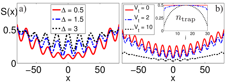
Figure 10: a) TOF for a non-ideal Kitaev chain where $J\neq\Delta$. b) Influence of an external harmonic trapping potential $H_{\mathrm{trap}}=-V_{t}\sum_{x}((L-1)/2-x)^{2}a^{\dagger}_{x}a_{x}$ on the TOF signal for a system of $L=30$ sites and $\Delta=1.2J$. In the inset we show the density for different values of $V_{t}$ in units of $J$. As long as the density of the system is not too inhomogeneous only the amplitude of the signal is affected by the external confinement. (see main text).

5 Spectroscopy

While TOF imaging allows to detect the existence and number of Majorana fermions in an AMO setup, the combination of a spectroscopic setup with TOF allows to measure not only the energy of the Majorana states but also their wave functions. (The use of spectroscopic RF absorption spectra to detect Majorana modes in $2D$ $p$-wave superconductors was considered in Ref. [25].) Consider a $1D$ lattice with two bands [modes $a_{j}$ ($b_{j}$) in the upper (lower) band] separated by an energy difference $\Delta E_{b}$. In the lower band we realize the Hamiltonian $H$, while the fermions can hop freely with the hopping amplitude $j$ in the upper band. The full Hamiltonian reads $H_{0}=H+H_{up}$, where $H_{up}=j\sum_{l=1}^{L}(b_{l}^{\dagger}b_{l+1}+h.c.)+\Delta E_{b}\sum_{l=1}^{L}b_{l}^{\dagger}b_{l}$. We then couple upper and lower bands on the first and the last sites of an open chain via a time-dependent perturbation $V(t)=V_{0}(b_{1}^{\dagger}a_{1}+b_{L}^{\dagger}a_{L})e^{-i\Omega t}+h.c.$ (see Fig. 11a) and measure the momentum distribution in the upper band as a function of the frequency $\Omega$, e.g., via TOF imaging.

Let us assume first that $J_{2}=\Delta_{2}=0,J_{1}=\Delta_{1}$ (ideal Kitaev chain) in the lower band. Then, the Hamiltonian $H$ is diagonal in the Bogoliubov quasiparticle basis $\tilde{a}_{l}=(a_{l}^{\dagger}-a_{l}+a_{l+1}^{\dagger}-a_{l+1})/2=(c_{2l+1}+ic_{2l})/2$, $H=2J_{1}\sum_{l=1}^{L-1}\tilde{a}_{l}^{\dagger}\tilde{a}_{l}$, and its ground state is two-fold degenerate, with the ground states $|G_{+}\rangle$ and $|G_{-}\rangle$ having different fermionic parity.

We can now rewrite the external perturbation in terms of quasiparticle operators $\tilde{a}_{l}$ and Majorana operators $\gamma_{L}$, $\gamma_{R}$ using $a_{1}=(\gamma_{L}+\tilde{a}_{1}^{\dagger}-\tilde{a}_{1})/2$, and $a_{L}=(\tilde{a}_{L-1}^{\dagger}+\tilde{a}_{L-1}-i\gamma_{R})/2$. Choosing the even parity ground state $|G_{+}\rangle$ as an initial state and using $\gamma_{L}|G_{\pm}\rangle=|G_{\mp}\rangle$ and $\gamma_{R}|G_{\pm}\rangle=\pm i|G_{\mp}\rangle$, a straightforward application of the standard time-dependent perturbation theory results in the following the upper band momentum distribution:

$$\langle n_{k}(t,\Omega)\rangle=V_{0}^{2}L^{-1}(n_{0}+n_{1}),$$ (6)

$$n_{0}=A_{0}f_{t}(\varepsilon_{k}-\Omega\hbar),\;\;\;\;\;n_{1}=f_{t}(\varepsilon_{k}+2J-\Omega\hbar),$$

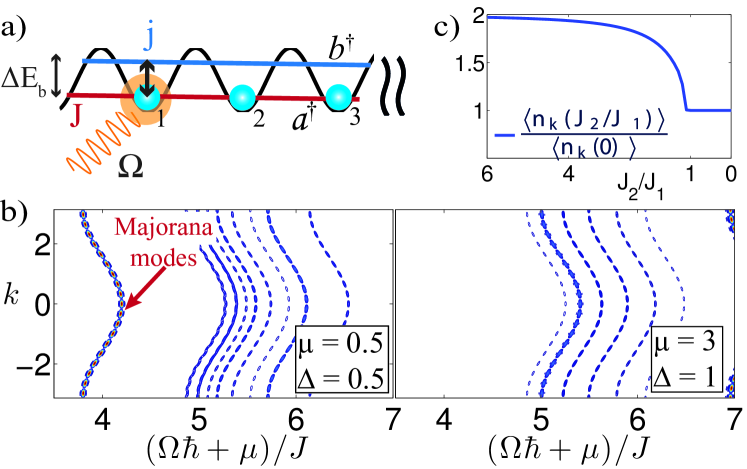
Figure 11: a) Spectroscopic detection of Majorana modes in a two-band lattice (see text). b) The momentum distribution of atoms in the upper band ($\Delta E_{b}=4J,j=0.1J$) reveals the presence (left) or absence (right) of Majorana modes (see text). c) From the strength of the signal $\langle n_{k}\rangle$ at resonance (here: $k=\pi/2$) we can deduce the number of Majorana modes.

where we have introduced the notation $A_{0}=[m_{+}(d)-m_{-}(d)]\sin^{2}\frac{k}{2}(L-1)+m_{-}(d)$ and $f_{t}(x)=4\sin^{2}(xt/2\hbar)/x^{2}$. Further, $\varepsilon_{k}=\Delta E_{b}+2j\cos k$ is the dispersion in the upper band and $m_{\pm}(d)$ denote the initial occupation of the even/odd parity subspace in the lower band. The contribution $n_{0}$ corresponds to a parity flip in the lower band (no energy cost) and the creation of an excitation (particle) in the upper band (energy $\varepsilon_{k}$). Thus, the absorption peak at $\hbar\Omega=\varepsilon_{k}$ in $n_{0}$ indicates the ground state degeneracy. The edge-edge Majorana correlation length is encoded in the oscillation period. The term $n_{1}$ results from the creation of excitations in both upper (energy $\varepsilon_{k}$) and lower (energy $2J$) band. The corresponding absorption peak is located at $\hbar\Omega=2J+\varepsilon_{k}$, providing the direct measurement of the pairing energy gap ($2J$ here) from the distance between the two peaks. Thus, the topologically non-trivial phase leads to a clear signal at $\Omega\hbar=2J$ (for $\mu\neq 0$ one has to replace $\hbar\Omega\rightarrow\hbar\Omega-\mu$, cf. Fig. 11b). Note that this setup allows to detect the presence of the zero energy Majorana subspace independently of its purity. Further, the number of Majorana modes is encoded in the strength of the resonance signal for a fixed momentum $k$. In Fig. 11c we present the results for the Hamiltonian $H$ with $J_{\alpha}=|\Delta_{\alpha}|$, $\phi=0$, where the perturbation is on sites $1,2,L-1$ and $L$. Starting from a state with four Majorana modes, we reduce the ratio $J_{2}/J_{1}$. At the transition point, the amplitude of the resonance signal $\langle n_{k=\pi/2}\rangle$ drops to half its magnitude indicating the disappearance of two of the Majorana modes. If we go away from the ideal case, the quasiparticle operators and the corresponding matrix elements can be determined numerically.

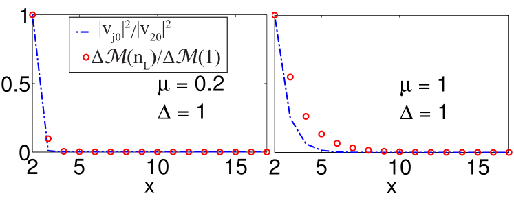
Figure 12: Measurement of the localization length of the Majorana mode via spectroscopy (see main text).

With a slight modification of the above setup one can also probe the localized character of the Majorana zero modes. Namely, we apply the perturbation to the first $n_{L}$ sites: $V^{(n_{L})}(t)=V_{0}\sum_{j=1}^{n_{L}}a_{j}^{\dagger}b_{j}e^{i\Omega t}+h.c.$. The corresponding momentum distribution in the upper band is now

$$\langle n_{k}({\Omega},t)\rangle=\frac{V_{0}^{2}}{L}\sum_{\nu=0}^{L-1}f_{t}(E_{\nu}+\epsilon_{k}-\Omega\hbar)\left|\sum_{j=1}^{n_{L}}e^{ikj}v_{j\nu}\right|^{2},$$ (7)

where $v_{jl}$ are the coefficients of the Bogoliubov transformation to the quasiparticle operators $\tilde{a}_{\nu}$ ($\nu$ labels the quasiparticle modes with energies $E_{\nu}$) in the lower band, $a_{i}=\sum_{j}(u_{i\nu}\tilde{a}_{\nu}-v_{i\nu}^{\ast}\tilde{a}_{\nu}^{\dagger})$, which diagonalizes $H$. Let us now consider $k=0$ and the external frequency being in resonance with the lowest energy ($\nu=0$ Majorana) level, $\Omega=\Omega_{r}=\Delta E_{b}+\epsilon_{k=0}$. In this case, only the Majorana mode is excited in the lower band, and one has $\langle n_{k=0}(\Omega_{r},t)\rangle\sim\left|\sum_{j=1}^{n_{L}}v_{j0}\right|^{2}\equiv\mathcal{M}(n_{L})$. The localized character of the Majorana mode can now be established by looking at the dependence of $\langle n_{k=0}(\Omega_{r},t)\rangle$ on the number of sites $n_{L}$ affected by the perturbation. To be more specific, the absolute change of $\mathcal{M}(n_{L})$ when $n_{L}$ is increased by one, $\Delta\mathcal{M}(n_{L})=\left|\mathcal{M}(n_{L}+1)-\mathcal{M}(n_{L})\right|$, is expected to be $\Delta\mathcal{M}(n_{L}>1)=0$ for the ideal Kitaev chain and $\Delta\mathcal{M}(n_{L})\sim\exp(-n_{L}/l_{\mathrm{loc}})$ for a generic one. This is reflected in a comparison of the normalized quantity $\Delta\mathcal{M}(n_{L})/\Delta\mathcal{M}(1)$ (red circles) with the normalized wave function of the Majorana mode, $\left|v_{j0}\right|^{2}/\left|v_{20}\right|^{2}$ (dashed) as shown in Fig. 12.

6 Probing Majorana fermions in $2D$.

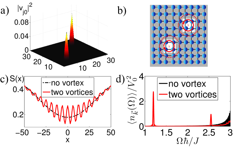
Figure 13: a) Spatial distribution of the Majorana modes in the vicinity of two vortices imprinted on a $p_{x}+ip_{y}$-superfluid for $\mu=2J$ on a $32\times 32$ lattice. b) A shade (grey) is introduced to enhance the signal contrast for the TOF (c) and spectroscopic (d) detections ($\Delta E_{b}=J,j=0.1J$).

In the last Sections we have presented methods to prepare and detect Majorana fermions in a one-dimensional model system. Note, however, that the proposed detection methods are universal and can be applied to other systems. As an illustration, we consider a $2D$ $p_{x}+ip_{y}$ superfluid, as it was proposed in  [33, 38] with Hamiltonian $H_{S}=H_{hopp}+H_{pair}+H_{\mu}$, with a NN hopping $H_{hopp}$, a pairing term $H_{pair}=\sum_{\mathbf{x},\mathbf{y}}\Delta_{\mathbf{x},\mathbf{y}}a_{\mathbf{x}}^{\dagger}a_{\mathbf{y}}^{\dagger}+h.c.$ where $\Delta_{\mathbf{x},\mathbf{y}}=\Delta_{x}(\delta_{\mathbf{y},\mathbf{x}+\mathbf{e}_{1}}+i\delta_{\mathbf{y},\mathbf{x}+\mathbf{e}_{2}})$, and $H_{\mu}=-\mu\sum_{\mathbf{x}}a_{\mathbf{x}}^{\dagger}a_{\mathbf{x}}$. The fermionic operators $a_{\mathbf{x}}$ are defined on a $2D$ (square) lattice and the vectors $\mathbf{e}_{1,2}$ are two independent elementary lattice translations. We introduce two vortices (each with vorticity $1$) via a position dependent order parameter $\Delta_{\mathbf{x}}=|\Delta|e^{i\phi(x)}$, which can be written onto the superfluid by phase imprinting in the Raman process [26].

For $\left|\mu\right|\ll 4J$ we have a topological ground state supporting two Majorana modes located in the vicinity of the two vortices (cf. Fig. 13 a). The comparison of the TOF signal with and without vortices (Fig. 13c) shows that the presence of the Majorana modes leads to an oscillatory behavior of the density $\langle n(x)\rangle$ at the detector. Again, the contrast of the signal is enhanced by shading all but a small region near the vortices (Fig. 13b). To detect the Majorana modes in the spectroscopic setup, we apply an external perturbation $V(t)=V_{0}\sum_{\mathbf{x}\in\Lambda}a_{\mathbf{x}}b_{\mathbf{x}}^{\dagger}e^{-i\Omega t}+h.c.$, where $\Lambda$ includes the lattice sites inside a $w\times w$ small regions around the vortices (here: $w=3$). The resulting momentum distribution in the upper band $\langle n_{k_{x},k_{y}}\rangle$ for $k_{x,y}=\frac{\pi}{32}$ is depicted in Fig. 13d. The presence of the Majorana modes leads to a clear signal at $\Omega\hbar/J=\varepsilon_{\frac{\pi}{32},\frac{\pi}{32}}/J\approx 1.19$ that is absent in a vortex-free setting.

7 Summary

In this work we have presented various techniques that allow for an unambiguous detection of atomic Majorana fermions and topological order with standard quantum optical tools, as time-of-flight imaging and spectroscopic techniques within our framework. To this end, we have introduced a one-dimensional model system that allows for an AMO realization and provides, due to its rich topological phase diagram, and ideal playground to test our ideas. Since some of our detection schemes require the preparation of a ground state with a definite parity, we have further provided a protocol that allows to achieve this goal. In addition, our detection techniques are universal in the sense that they can be used to detect atomic Majorana fermions in any dimension and geometry, as we have illustrated by the example of a $2D$ $p_{x}+ip_{y}$ superfluid.

8 Acknowledgments

We thank E. Rico for helpful discussions. We acknowledge support by the Austrian Science Fund (FWF) through SFB FOQUS and the START grant Y 581-N16 (S. D.), the European Commission (AQUTE), the Institut fuer Quanteninformation GmbH and the DARPA OLE program.

References

References

- [1] S. Ryu, A. P. Schnyder, A. Furusaki, and A. W. W. Ludwig, New Journal of Physics, 12(6), 065010 (2010).
- [2] A. P. Schnyder, S. Ryu, A. Furusaki, and A. W. W. Ludwig, Phys. Rev. B, 78, 195125 (2008).
- [3] A.Y. Kitaev, AIP Conf. Proc., 1134, 22 (2008).
- [4] X.-L. Qi, T. L. Hughes, and S.-C. Zhang, Phys. Rev. B, 78, 195424, (2008).
- [5] M. R. Zirnbauer, J. Math. Phys., 37,4986, (1996).
- [6] A. Altland and Martin R. Zirnbauer, Phys. Rev. B, 55, 1142 (1997).
- [7] J. C. Y. Teo and C. L. Kane, Phys. Rev. B, 82, 115120 (2010).
- [8] V. Gurarie, Phys. Rev. B, 83, 085426 (2011).
- [9] A. M. Essin and V. Gurarie, Phys. Rev. B, 84, 125132 (2011).
- [10] Jay D. Sau, Roman M. Lutchyn, S. Tewari, and S. Das Sarma, Phys. Rev. Lett., 104, 040502 (2010).
- [11] J. Alicea, Y. Oreg, G. Refael, F. von Oppen, and M. P. A. Fisher, Nature Physics, 7, 412 (2011).
- [12] S. Tewari, S. Das Sarma, C. Nayak, C. Zhang, and P. Zoller, Phys. Rev. Lett., 98, 010506 (2007).
- [13] L. Fu and C. L. Kane, Phys. Rev. Lett., 102, 216403 (2009).
- [14] L. Fu, Phys. Rev. Lett., 104, 056402 (2010).
- [15] J. D. Sau, S. Tewari, R. M. Lutchyn, T. D. Stanescu, and S. Das Sarma, Phys. Rev. B, 82, 214509 (2010).
- [16] A. R. Akhmerov, J. Nilsson, and C. W. J. Beenakker, Phys. Rev. Lett., 102, 216404 (2009).
- [17] T. D. Stanescu, R. M. Lutchyn, and S. Das Sarma, Phys. Rev. B, 84, 144522 (2011).
- [18] V. Mourik, K. Zuo, S. M. Frolov, S. R. Plissard, E. P. A. M.Bakkers and L. P. Kouwenhoven, Science, 1222360 (2012).
- [19] N. Goldman, I. Satija, P. Nikolic, A. Bermudez, M. A. Martin-Delgado, M. Lewenstein, and I. B. Spielman, Phys. Rev. Lett., 105, 255302 (2010).
- [20] J. Levinsen, N. R. Cooper, and G. V. Shlyapnikov, Phys. Rev. A, 84, 013603 (2011).
- [21] T. D. Stanescu, V. Galitski, and S. Das Sarma, Phys. Rev. A, 82, 013608 (2010).
- [22] K. Sun, Z. Gu, H. Katsura, and S. Das Sarma, Phys. Rev. Lett., 106, 236803 (2011).
- [23] L. Jiang, T. Kitagawa, J. Alicea, A. R. Akhmerov, D. Pekker, G. Refael, J. I. Cirac, E. Demler, M. D. Lukin, and P. Zoller, Phys. Rev. Lett., 106, 220402 (2011).
- [24] S. Diehl, E. Rico, M. A. Baranov, and P. Zoller, Nat. Phys., 7, 971 (2011).
- [25] Detection methods for Majorana fermions in the condensed matter systems have been proposed by Yaacov E. Kraus, Assa Auerbach, H. A. Fertig, and S. H. Simon, Phys. Rev. B, 79, 134515 (2009) and E. Grosfeld, N. R. Cooper, A. Stern, and R. Ilan, Phys. Rev. B, 76, 104516 (2007).
- [26] C. Weitenberg, M. Endres, J. F. Sherson, M. Cheneau, P. Schauß, T. Fukuhara, I. Bloch, and S. Kuhr, Nature, 471, 319 (2011).
- [27] J. Simon, W. S. Bakr, R. Ma, M. E. Tai, P. M. Preiss, and M. Greiner, Nature,472, 307 (2011).
- [28] I. Bloch, J. Dalibard, and W. Zwerger, Rev. Mod. Phys., 80, 885 (2008).
- [29] E. Zhao, N. Bray-Ali, C. J. Williams, I. B. Spielman, and I. I. Satija, Phys. Rev. A, 84, 063629 (2011).
- [30] E. Alba, X. Fernandez-Gonzalvo, J. Mur-Petit, J. K. Pachos, and J. J. Garcia-Ripoll, Phys. Rev. Lett., 107, 235301 (2011).
- [31] G. Juzeliūnas and I. Spielman, Physics, 4, 99 (2011).
- [32] A. Y. Kitaev, Physics-Uspekhi, 44(10S), 131, (2001).
- [33] D. A. Ivanov, Phys. Rev. Lett., 86, 268 (2001).
- [34] W. Ketterle and M. W. Zwierlein, Nuovo Cimento Rivista Serie, 31, 247 (2008).
- [35] A. J. Leggett, Quantum Liquids: Bose Condensation and Cooper Pairing in Condensed-Matter Systems, Oxford University Press, USA, 2006.
- [36] S. Bravyi, M. B. Hastings, F. Verstraete, Phys. Rev. Lett. 97, 050401 (2006).
- [37] J. Eisert, T. J. Osborne, Phys. Rev. Lett. 97, 150404 (2006).
- [38] N. Read and D. Green, Phys. Rev. B, 61, 10267 (2000).