Abelian Manna model in three dimensions and below

Abstract

The Abelian Manna model of self-organized criticality is studied on various three-dimensional and fractal lattices. The exponents for avalanche size, duration and area distribution of the model are obtained by using a high-accuracy moment analysis. Together with earlier results on lower-dimensional lattices, the present results reinforce the notion of universality below the upper critical dimension and allow us to determine the coefficients of an $\epsilon$-expansion. By rescaling the critical exponents by the lattice dimension and incorporating the random walker dimension , a remarkable relation is observed, satisfied by both regular and fractal lattices.

I Introduction

Critical phenomena play an important role in our understanding of complex systems in nature. One of the key features of critical systems is the notion of universality Stanley (1999). It suggests common underlying mechanisms of seemingly different phenomena and also allows us to study complicated natural systems through analysis of simple (numerical) models. A huge number of numerical models have been proposed to study different features of critical systems. Traditionally, those systems require external fine tuning of control parameter to critical point. However, many models exhibit the features of the crititcal state without the need of tuning a control parameter, which is known as self-organized criticality Bak et al. (1987). While models of traditional critical phenomena have been very well studied both analytically and numerically, and important results including exact ones have been obtained (e.g. Syôzi, 1951), little success has been achieved for self-organized critical phenomena. One example of such models is the Manna model Manna (1991) which has so far defied any attempt for an analytical approach, but has been studied extensively numerically. Yet the question of universality seems to have been overlooked in the literature in a very fundamental point: Does the Manna model display the same critical behaviour on different lattices of the same dimension? Recent extensive numerical studies Huynh et al. (2011) of the Abelian version of the Manna model Manna (1991); Dhar (1999a, b) on various lattices in integer dimensions $1$ and $2$ provide very strong support for the model’s universal behaviour. The situation, however, is more complicated in non-integer dimensions Huynh et al. (2010). Thus, it would be of great interest to see if the results in fractal dimensions can be reconciled with those in integer dimensions in a systematic manner.

Our motivation for this study is to provide a complete numerical picture of the Manna model. Three main results are reported: Firstly, we confirm universality in three dimensions, i.e. the independence of critical exponents and moment ratios from the detailed structure of the underlying lattice. This allows us, secondly, to firmly estimate the coefficients of an $\epsilon$-expansion for the exponents. Thirdly, we identify a general scaling relation unifying critical behaviour on regular and fractal lattices.

II Model and observables

The Abelian Manna model Manna (1991); Dhar (1999a, b); Huynh et al. (2011) is defined on a lattice of dimension $d$ with $N$ sites and linear extent $L$, where $N\propto L^{d}$ asymptotically. Each site $i$ has a local degree of freedom $z_{i}\geq 0$ which can be thought of as the number of particles residing at that site. If $z_{i}>1$, the site is said to be active or unstable, otherwise it is stable. The system evolves by driving and subsequently fully relaxing it. Driving: The system is “charged” by picking a site $j$ randomly and uniformly and increasing $z_{j}$ by $1$. Relaxation: An unstable site $i$ is picked randomly and uniformly; its particle number is reduced by $2$ and the particle number of two of its $q_{i}$ neighbours, which are chosen independently and at random (possibly the same one twice), is increased by $1$, thereby possibly rendering them unstable. Dissipation takes place only when relaxing boundary sites transfer particles to $q^{(v)}$ virtual neighbours “outside” the lattice. These virtual neighbours cannot topple themselves and are chosen so that the topology of the finite lattice corresponds to that of an “offcut” from an infinite lattice. Relaxation of unstable sites continues until there are no unstable sites left. Only then the system is driven again, known as a separation of time scales. The number of topplings between two driving steps is the size $s$ of the “avalanche” and the number of distinct sites toppling is the area $a$. The duration $t$ of the avalanche is measured on the microscopic time scale, which advances in steps of $1/N_{a}$, where $N_{a}$ is the instantaneous number of active sites, mimicking a Poissonian decay of active sites. The moments of the observables mentioned above are measured in the stationary state, which is reached after a generously estimated transient. A number of (asymptotic) key characteristics of the lattices are listed in Table III, such as the average number of neighbours $\overline{q}$, the average number of virtual neighbours $\overline{q^{(v)}}$ among sites with at least one virtual neighbour, and the particle density $\zeta$ in the stationary state.

The probability densities $\mathcal{P}^{(x)}\left(x,L\right)$ of the observables, $x\in\{s,a,t\}$, are expected to display finite size scaling

$$\mathcal{P}^{(x)}\left(x,L\right)=a_{x}x^{-\tau_{x}}\mathcal{G}_{x}\left(\frac{x}{b_{x}L^{D_{x}}}\right),$$ (1)

provided that $L\gg 1$ and $x\gg x_{0}$ for some lower cutoff $x_{0}$. The metric factors $a_{x}$ and $b_{x}$ are not expected to be universal Privman et al. (1991), whereas the exponent $D_{x}$ should only depend on the dimension and $\tau_{x}$ on the dimension and the boundary conditions Nakanishi and Sneppen (1997). The universal scaling function $\mathcal{G}_{x}$ is characterised below by moment ratios. For $n>\tau_{x}-1$, the moments scale asymptotically like $\left\langle x^{n}\right\rangle\propto L^{\mu_{n}^{(x)}}$ with $\mu_{n}^{(x)}=D_{x}(1+n-\tau_{x})$. For historic reason, the exponents are denoted as $D$ (for $D_{s}$), $\tau$ (for $\tau_{s}$), $z$ (for $D_{t}$), and $\alpha$ (for $\tau_{t}$).

Five three-dimensional and five fractal lattices are employed in this study. The three-dimensional lattices Ashcroft and Mermin (1976) are built upon the standard simple cubic (SC) lattice. The body centered cubic (BCC) and face centered cubic (FCC) lattices are also studied with next nearest neighbour interactions (BCCN and FCCN, respectively). The total number of sites $N$ of all five lattices are chosen to be as close as possible to one another. Typically, six system sizes ranging from $N=181^{3}$ to $N=1024^{3}$ are used. A total of approximately 50,000 CPU hours have been spent on three-dimensional systems.

The key features of the fractal lattices are listed in Table III. Of those the lesser known semi-inverse square triadic Koch (SSTK) lattice Huynh and Chew (2011); Addison (1997) has Hausdorff dimension $d=\ln 5/\ln 3$ and is exemplified in Fig. 1. Of particular interest is the Sierpinski tetrahedron (SITE) lattice, which is the three-dimensional version of the well-known Sierpinski gasket, based on tetrahedra instead of triangles. Its fractal dimension is $d=2$ and thus allows a direct comparison to regular two-dimensional lattices. The strongly anisotropic extended Sierpinski gasket (EXGA, $d=\ln 6/\ln 2$) is obtained by stacking $L$ copies of a Sierpinski gasket on top of one another and applying periodic boundary conditions. Finally, the arrowhead (ARRO, $d=\ln{3}/\ln{2}$) and the crab (CRAB, $d=\ln{3}/\ln{2}$) lattices are the same as the ones used in Huynh et al. (2010). Typically, four system sizes corresponding to iterations from $6$ to $9$ are used for all fractal lattices ($5$ to $8$ for SSTK). A total of approximately 75,000 CPU hours have been spent on fractal lattices.

Figure 1: Semi-inverse square triadic Koch lattice at iteration 3.

III Results

Details of the Monte Carlo simulation, the fitting procedures and the derivation of the error bars can be found in Huynh et al. (2011). In short, individual moments $\left\langle x^{n}\right\rangle(L)$ are fitted against the system size $N\propto L^{d}$ to obtain the scaling exponent $\mu_{n}^{(x)}/d$ using a power law with corrections. For regular three-dimensional lattices, the form of fitting function used for avalanche size and duration is

$$\left\langle x^{n}\right\rangle(N)=A_{n}^{(x)}N^{\mu_{n}^{(x)}/d}+B_{n}^{(x)}N^{\mu_{n}^{(x)}/d-0.25}$$ (2)

and for avalanche area is

$$\left\langle a^{n}\right\rangle(N) = A_{n}^{(a)}N^{\mu_{n}^{(a)}/d}+B_{n}^{(a)}N^{\mu_{n}^{(a)}/d-0.25}$$ (3)

$$+ C_{n}^{(a)}N^{\mu_{n}^{(a)}/d-0.5}.$$

For fractal lattices we use Eq. (2) in Huynh et al. (2010)

$$\left\langle x^{n}\right\rangle(N) = A_{n}^{(x)}N^{\mu_{n}^{(x)}/d}+B_{n}^{(x)}N^{\mu_{n}^{(x)}/d-1}$$ (4)

$$+ C_{n}^{(x)}N^{\mu_{n}^{(x)}/d-2}.$$

The estimated scaling exponents $\mu_{n}^{(x)}$ are then linearly fitted against the moment orders $n$ ($n=2,3,4,5$ for all except for $\mu_{n}^{(s)}$ in three dimensions with $n=2,3,4$). The slope gives the exponent $D_{x}$ and the interception with the abscissa gives the exponent $\tau_{x}$, except for $\tau_{s}$ of three-dimensional lattices, whose estimate is obtained by employing the exact relation $D_{s}(2-\tau_{s})=2$. Although the relative errors are as small as $3\times 10^{-3}$, we were unable to adjust the fitting scheme as to recover $\mu_{1}^{(s)}=2$ within less than $3$ standard deviations.

The quality of all data fitting reported in this work is assessed by the goodness-of-fit $q$ Press et al. (2007), which is considered good if $q>0.1$, otherwise they are marked by $[\cdot]$. Tables III and III summarise the estimated critical exponents, all obtained with $q>0.5$. For regular lattices, our results compare well with the literature Ben-Hur and Biham (1996); Lübeck (2000); Pastor-Satorras and Vespignani (2001) (also Alava and Muñoz (2002); Lübeck and Heger (2003a) for absorbing state phase transitions), although some variability and discrepancy is observed in particular for $z$ which may be explained by the use of slightly different model definitions (and dynamics) by other authors. A number of scaling relations (see below) are confirmed, such as $-\Sigma_{x}=D_{x}(\tau_{x}-1)=D_{y}(\tau_{y}-1)=-\Sigma_{y}$ Lübeck (2000). Overall estimates are included in Table III, the correlation of $\Sigma_{s}$, $\Sigma_{t}$ and $\Sigma_{a}$ is taken into account by multiplying their respective errors by $\sqrt{3}$.

Table 1: Key features of the three-dimensional ($d=3$) lattices considered in this work. The random walker dimension $d_{w}$ is $2$ for every regular lattice ben-Avraham and Havlin (2000). The asymptotic site averaged number of nearest neighbours is $\overline{q}$, with boundary sites having on average $\overline{q^{(v)}}$ neighbours missing (virtual neighbours Huynh et al. (2011)). The stationary particle density, equal to the average density of (singly) occupied sites, is given by $\zeta$.

Lattice	$d$	$d_{w}$	$\overline{q}$	$\overline{q^{(v)}}$	$\zeta$
SC	3	2	6	1	[0.622325(1)]
BCC	3	2	8	4	[0.600620(2)]
BCCN	3	2	14	5	[0.581502(1)]
FCC	3	2	12	4	[0.589187(3)]
FCCN	3	2	18	5	[0.566307(3)]

The moment ratios Binder (1981); Huynh et al. (2011) $g_{n}^{(x)}$ (to leading order) are independent of the system size and characterise the scaling function $\mathcal{G}_{x}$. The fitting of moment ratios follows a similar procedure as the avalanche exponents, using

$$g_{n}^{(x)}=\mathcal{A}_{n}^{(x)}+\mathcal{B}_{n}^{(x)}N^{-0.25}+\mathcal{C}_{n}^{(x)}N^{-0.5}.$$ (5)

Together with the avalanche exponents, they provide very strong support for universality in regular lattices. Table III lists the overall moment ratios based on five three-dimensional lattices.

Surprisingly (see Huynh et al. (2011) for the same phenomenon in one and two dimensions), the amplitudes of the leading order of the moments of the avalanche area seem to be universal. We found

$$\begin{array}[]{rcl}\left\langle a^{1}\right\rangle&=&[0.202(4)]N^{\tilde{\mu}_{1}^{(a)}}\\ \left\langle a^{2}\right\rangle&=&0.0151(15)N^{\tilde{\mu}_{2}^{(a)}}\\ \left\langle a^{3}\right\rangle&=&0.0027(6)N^{\tilde{\mu}_{3}^{(a)}}\\ \left\langle a^{4}\right\rangle&=&0.00055(19)N^{\tilde{\mu}_{4}^{(a)}}\\ \left\langle a^{5}\right\rangle&=&0.00012(6)N^{\tilde{\mu}_{5}^{(a)}}\\ \end{array}$$ (6)

with universal $\tilde{\mu}_{n}^{(a)}=n+1-1.4396(8)$ across the three-dimensional lattices introduced above. It is obviously crucial to consider $\left\langle a^{n}\right\rangle$ as a function of $N$, as fitting against $L=\lambda N^{1/d}$ leads to different amplitudes, because $\lambda$ varies from lattice to lattice.

Table 2: Key features of the fractal lattices studied, as listed in Table III for the three-dimensional ones. The random walker dimensions are exactly known or derived (in case of SSTK estimated) using the methods described in Huynh et al. (2010).

Table 3: Avalanche exponents of five three-dimensional lattices. The estimates for $\tau$ and $D(\tau-1)$ are obtained from $D$ via the exact scaling relation $D(2-\tau)=2$. Identities $D_{a}=d$ and $\mu_{1}^{(s)}=2$ are used to validate the fitting scheme.

Table 4: Overall estimates of moment ratios for three-dimensional lattices.

Table 5: Avalanche exponents of five fractal lattices.

Table 6: Summary of exponents in all dimensions.

III.1 Regular lattices

All critical exponents including previous results Huynh et al. (2011) are summarised in Table III. Firstly, on regular lattices, a relation between $D_{x}$, $\tau_{x}$ and the dimension $d$ can be obtained by fitting exponents against a proposed function $D_{x}=f_{x}(d)$ and $\tau_{x}=h_{x}(d)$. With six exponents six functions are to be determined, which, however, are related by scaling laws. They are

$$D(2-\tau)=2$$ (7)

on regular lattices (exact Nakanishi and Sneppen (1997)), $D_{a}=d$ (assumed to hold on regular lattices by Ben-Hur and Biham (1996); Chessa et al. (1999), and in the present case confirmed for fractal lattices) and $D_{x}(\tau_{x}-1)=-\Sigma_{x}$ with $\Sigma_{a}=\Sigma_{s}=\Sigma_{t}$ (narrow distribution assumption Jensen et al. (1989)). Using $\tau=2-2/D$, $D_{a}=d$, $\tau_{a}=1+(D-2)/d$, and $\alpha=1+(D-2)/z$, there are thus only two functions to determine, which are best expressed in terms of $\epsilon=4-d$ since $d_{c}=4$ is the upper critical dimension Lübeck and Heger (2003a), where the exponents are known exactly. Writing $D=4-c_{1}^{(s)}\epsilon+c_{2}^{(s)}\epsilon^{2}+\ldots$, at most two amplitudes $c_{i}^{(s)}$ can reasonably be determined on the basis of the three data points available. A fit of $D$ with only a linear term produces a very poor goodness-of-fit, which does not improve satisfactorily by including a term quadratic in $\epsilon$. Omitting the quadratic gives

$$D=4-0.654(6)\epsilon+0.0079(10)\epsilon^{3}$$ (8)

with $q\approx 0.095$ ($c_{1}^{(s)}=0.60(4)$, $c_{2}^{(s)}=-0.05(3)$, $c_{3}^{(s)}=-0.019(7)$ with three terms). Similarly, $z=2-0.239(4)\epsilon+0.0056(6)\epsilon^{3}$, however with nearly vanishing goodness-of-fit.

III.2 Fractal lattices

Attempting to unify the above $\epsilon$-expansion obtained for regular lattices with the results for fractals with Hausdorff dimension $d$ is bound to fail, which is immediately clear when comparing the exponents found for the fractal SITE lattice ($d=2$, Table III) with those for the regular two-dimensional lattices, or the ARRO and the CRAB lattice, Table III, which have the same Hausdorff dimension. As is well understood, the basic scaling relation Eq. (7) is valid only for regular lattices and has to be generalised to

$$D(2-\tau)=d_{w}$$ (9)

with random walker dimension $d_{w}\geq 2$ ben-Avraham and Havlin (2000); Huynh et al. (2010).

It turns out, however, that $D$ is essentially a linear function of $d$ and $d_{w}$

$$D=ad+bd_{w}$$ (10)

with the same coefficients $a$ and $b$ for both, regular and fractal lattices, which can be extracted from the $\epsilon$-expansion obtained above with $d_{c}=4=2d_{w}$, because $d_{w}=2$ on regular lattices, $a=c_{1}^{(s)}$ and $b=2(1-c_{1}^{(s)})$, so that on the basis of Eq. (8) $a=0.654(6)$ and $b=0.692(12)$ or $a=0.60(4)$ and $b=0.80(8)$ depending on $c_{1}^{(s)}$. Fitting the data in Table III against Eq. (10) gives $a=[0.550(4)]$, $b=[0.822(3)]$, and a fitting with the constraint $b=2(1-a)$ from exactly known values of exponents at $d=d_{c}=4$ gives $a=[0.6061(5)]$, $b=[0.7878(10)]$. Figure 2 shows $D/d$ as a function of $d_{w}/d$ for all lattices listed in Table III. As expected from Eq. (10), fractal and regular lattices display essentially the same linear dependence $D/d=a+bd_{w}/d$. Above the upper critical dimension $d_{c}=4$ regular lattices attain their mean-field values, $D=4$, $\tau=3/2$ Lübeck (2004) and $d_{w}=2$, therefore following Eq. (10) with $a=0$ and $b=2$. One may wonder whether fractal lattices with Hausdorff dimension greater than $d_{c}=4$ have correspondingly exponents $D=2d_{w}$.

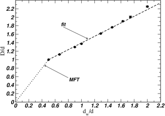
Figure 2: The data of Table III plotted in the form $D/d$ versus $d_{w}/d$ as suggested by Eq. (10). The dashed straight line is based on the estimates $a=[0.6061(5)]$ and $b=[0.7878(10)]$, the dotted line is the mean field theory, $a=0$, $b=2$.

The choice of rescaling exponent $D$ by dimension $d$ of the lattice is not random, but rather a natural choice, given that we perfomed all fitting of $\mu_{n}^{(x)}$ against the number of sites $N$ rather than the lattices’ linear length $L$ and multiplied the results by the Hausdorff dimension $d$. The gap exponents for the scaling in $N$ is $D/d$, which, as it turns out, displays a very systematic dependence on $d_{w}/d$.

Further investigation shows that $D/d$ fits very well to

$$\left(\frac{D}{d}\right)^{2}(\tau-\tilde{a})=\tilde{b}$$ (11)

with $\tilde{a}=1.020(2)$ and $\tilde{b}=0.481(3)$ for all lattices which results in

$$D=4-0.658(5)\epsilon+0.00962(13)\epsilon^{2}+0.00161(3)\epsilon^{3}+\cdots$$ (12)

using $D(2-\tau)=d_{w}=2$ for the regular ones.

The form of Eq. (11) was obtained by first fitting $\tau$ against $(D/d)^{\kappa}$, which gives a $\kappa$ deviating from $-2$ by less than $2\%$. The coefficient $\tilde{a}$ and $\tilde{b}$ are then fitted according to Eq. (11). Figure 3 compares that relation to results for lattices in all dimensions. In the same manner, a similar relation can be obtained for $z$ and $\alpha$,

$$\left(\frac{z}{d}\right)^{\frac{3}{2}}(\alpha-\tilde{a})=\tilde{b}$$ (13)

with $[\tilde{a}=0.936(2)]$ and $[\tilde{b}=0.3768(12)]$.

The above results suggest that the scaling in $N$ is more suitable for fractals than the scaling in $L$. We suspect this is related to $L$ not capturing the chemical distance, which is the distance particles need to travel on the lattice, whereas $L$ is measured as a Euclidean distance. By using $d_{w}$, which is sensitive to the chemical distance, and considering the scaling against $N$, which is a well-defined measure of the size for any lattice, we are able to determine the relations above.

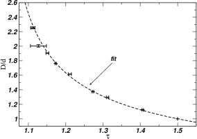
(a) Avalanche size exponents and fit, $D/d=(\tilde{b}/(\tau-\tilde{a}))^{1/2}$

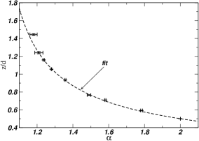
(b) Avalanche duration exponents and fit, $z/d=(\tilde{b}/(\alpha-\tilde{a}))^{2/3}$

Figure 3: Fit of the exponents in all dimensions (on regular and fractal lattices) against Eq. (11). The symbols represent the data in Table III, the dashed lines are the fits as described in the text, Eq. (11) and Eq. (13), respectively.

IV Conclusion

In conclusion, we studied Abelian Manna model on various three-dimensional and fractal lattices with the aim to provide a complete picture about the model below the upper critical dimension. The results confirm the consistent and robust universal behaviour of the Manna model across different, regular lattices, which allowed us to produce an $\epsilon$-expansion of avalanche exponents below the upper critical dimension. A relation between critical exponents and lattice dimension is observed which systematically reconciles integer dimensional with fractal lattices.

The authors are indebted to Andy Thomas, Dan Moore and Niall Adams for running the SCAN computing facility at the Department of Mathematics of Imperial College London. HNH thanks Lock Yue Chew for his support.

References

- Stanley (1999) H. E. Stanley, Rev. Mod. Phys. 71, S358 (1999).
- Bak et al. (1987) P. Bak, C. Tang, and K. Wiesenfeld, Phys. Rev. Lett. 59, 381 (1987).
- Syôzi (1951) I. Syôzi, Prog. Theor. Phys. 6, 306 (1951).
- Manna (1991) S. S. Manna, J. Phys. A: Math. Gen. 24, L363 (1991).
- Huynh et al. (2011) H. N. Huynh, G. Pruessner, and L. Y. Chew, J. Stat. Mech. 2011, P09024 (2011).
- Dhar (1999a) D. Dhar, Physica A 263, 4 (1999a).
- Dhar (1999b) D. Dhar (1999b), eprint arXiv:cond-mat/9909009.
- Huynh et al. (2010) H. N. Huynh, L. Y. Chew, and G. Pruessner, Phys. Rev. E 82, 042103 (2010).
- Privman et al. (1991) V. Privman, P. C. Hohenberg, and A. Aharony, in Phase Transitions and Critical Phenomena, edited by C. Domb and J. L. Lebowitz (Ann. Phys. (NY), New York, NY, USA, 1991), vol. 14, chap. 1, pp. 1–134.
- Nakanishi and Sneppen (1997) H. Nakanishi and K. Sneppen, Phys. Rev. E 55, 4012 (1997).
- Ashcroft and Mermin (1976) N. W. Ashcroft and N. D. Mermin, Solid State Physics (Harcourt College Publishers, 1976).
- Huynh and Chew (2011) H. N. Huynh and L. Y. Chew, Fractals 19, 141 (2011).
- Addison (1997) P. S. Addison, Fractals and Chaos: An illustrated course (Institute of Physics, London, UK, 1997).
- Press et al. (2007) W. H. Press, S. A. Teukolsky, W. T. Vetterling, and B. P. Flannery, Numerical recipes: the art of scientific computing (Cambridge University Press, Cambridge, UK; New York, 2007), 3rd ed.
- Ben-Hur and Biham (1996) A. Ben-Hur and O. Biham, Phys. Rev. E 53, R1317 (1996).
- Lübeck (2000) S. Lübeck, Phys. Rev. E 61, 204 (2000).
- Pastor-Satorras and Vespignani (2001) R. Pastor-Satorras and A. Vespignani, Eur. Phys. J. B 19, 583 (2001).
- Alava and Muñoz (2002) M. Alava and M. A. Muñoz, PRE 65, 026145 (2002).
- Lübeck and Heger (2003a) S. Lübeck and P. C. Heger, Phys. Rev. Lett. 90, 230601 (2003a).
- ben-Avraham and Havlin (2000) D. ben-Avraham and S. Havlin, Diffusion and reactions in fractals and disordered system (Cambridge University Press, Cambridge ; New York, 2000).
- Binder (1981) K. Binder, Phys. Rev. Lett. 47, 693 (1981).
- Lübeck and Heger (2003b) S. Lübeck and P. C. Heger, Phys. Rev. E 68, 056102 (2003b).
- Lübeck (2004) S. Lübeck, Int. J. Mod. Phys. B 18, 3977 (2004).
- Chessa et al. (1999) A. Chessa, H. E. Stanley, A. Vespignani, and S. Zapperi, Phys. Rev. E 59, R12 (1999).
- Jensen et al. (1989) H. J. Jensen, K. Christensen, and H. C. Fogedby, Phys. Rev. B 40, 7425 (1989).