The nuclear starburst in Arp 299-A: From the 5.0 GHz VLBI radio light-curves to its core-collapse supernova rate

Abstract

Context. The nuclear region of the Luminous Infra-red Galaxy Arp 299-A hosts a recent ($\simeq 10$ Myr), intense burst of massive star formation which is expected to lead to numerous core-collapse supernovae (CCSNe). Previous VLBI observations, carried out with the EVN at 5.0 GHz and with the VLBA at 2.3 and 8.4 GHz, resulted in the detection of a large number of compact, bright, non-thermal sources in a region $\!\!\!\phantom{\leq}\smash{\buildrel\over{\lower 2.67502pt\hbox{$\buildrel\lower 2.14001pt\hbox{$\displaystyle<$}\over{\sim}$}}}\,\,$150 pc in size.

Aims. We aim at establishing the nature of all non-thermal, compact components in Arp 299-A, as well as estimating its core-collapse supernova rate. While the majority of them are expected to be young radio supernovae (RSNe) and supernova remnants (SNRs), a definitive classification is still unclear. Yet, this is very relevant for eventually establishing the core-collapse supernova rate, as well as the star formation rate, for this galaxy.

Methods. We use multi-epoch European VLBI Network (EVN) observations taken at 5.0 GHz to image with milliarcsecond resolution the compact radio sources in the nuclear region of Arp 299-A. We also use one single-epoch 5.0 GHz Multi-Element Radio Linked Interferometer Network (MERLIN) observation to image the extended emission in which the compact radio sources –traced by our EVN observations– are embedded.

Results. We present the first 5.0 GHz radio light-curve (spanning $\sim$2.5 yr) of all compact components in the nuclear starburst of Arp 299-A. Twenty-six compact sources are detected, 8 of them are new objects not previously detected. The properties of all detected objects are consistent with them being a mixed population of CCSNe and SNRs. We find clear evidence for at least two new CCSNe, implying a lower limit to the CCSN rate of $\nu_{\rm SN}\!\!\!\phantom{\geq}\smash{\buildrel\over{\lower 2.67502pt\hbox{$\buildrel\lower 2.14001pt\hbox{$\displaystyle>$}\over{\sim}$}}}\,\,$0.80 SN/yr indicating that the bulk of the current star formation in Arp 299-A is taking place in the innermost $\sim 150$ pc. A few more objects show variability consistent with being recently exploded SNe, but only forecoming new observations will clarify this point. Our MERLIN observations trace a region of diffuse, extended emission which is cospatial to the region where all compact sources are found in our EVN observations. From this diffuse, non-thermal radio emission traced by MERLIN we obtain an independent estimate for the core-collapse supernova rate, which is in the range $\nu_{\rm SN}=0.40$ - $0.65$ SN/yr, in agreement with previous estimates and our direct estimate of the CCSN rate from the compact radio emission.

Conclusions. Our $\sim$2.5 yr monitoring of Arp 299-A has allowed us to obtain for the first time a direct estimate of the CCSN rate of $\nu_{\rm SN}\!\!\!\phantom{\geq}\smash{\buildrel\over{\lower 2.67502pt\hbox{$\buildrel\lower 2.14001pt\hbox{$\displaystyle>$}\over{\sim}$}}}\,\,0.80$ SN/yr for the innermost $\sim$150 pc of Arp 299-A.

1 Introduction

According to the $\Lambda$ cold dark matter hierarchical models of galaxy formation, more massive galaxies are assembled from smaller ones in a series of minor or major merger events (e.g. Toomre & Toomre, 1972). Nearby examples of merger galaxies are often associated with the class of Luminous, LIRG with $10^{11}L_{\odot}\leq L_{\rm IR}<10^{12}L_{\odot}$, and Ultra Luminous Infrared Galaxies, ULIRG with $L_{\rm IR}\geq 10^{12}L_{\odot}$ (Soifer et al., 1989; Sanders & Mirabel, 1996). Galaxy interactions and mergers can produce stellar bars and/or enhanced spiral structure that drive ample quantities of molecular gas and dust into the circumnuclear regions of (U)LIRGs, triggering massive star formation and possibly accretion onto a supermassive black hole (e.g. Di Matteo et al., 2007)

Coupling high sensitivity with a wide range of angular resolutions, and being unaffected by dust obscuration, radio observations provide an important and unique tool to investigate the nuclear components of (U)LIRGs. In particular, Very Long Baseline Interferometry (VLBI) observations allowed to resolve the nuclear component of local (U)LIRG, detecting tens of compact objects in the merger nuclei of Arp 220 and Arp 299 (Smith et al., 1998; Rovilos et al., 2003; Lonsdale et al., 2006; Parra et al., 2007; Neff et al., 2004; Pérez-Torres et al., 2009; Ulvestad, 2009; Pérez-Torres et al., 2010). The non-thermal origin of these compact sources is confirmed by their high brightness temperatures, implying that most of them are young core-collapse (radio) SNe (CCSNe) or supernova remnants (SNRs). Radio spectral index and flux density variability can be used to distinguish between the two classes of sources (Parra et al., 2007), but the results are usually not conclusive for all sources, and therefore the number of observed CCSNe is uncertain. This is an important parameter, as the observed rate at which massive stars ($M\!\!\!\phantom{\geq}\smash{\buildrel\over{\lower 2.67502pt\hbox{$\buildrel\lower 2.14001pt\hbox{$\displaystyle>$}\over{\sim}$}}}\,\,8M_{\odot}$) explode as CCSNe can be used as a direct measurement of the current star formation rate (SFR) in galaxies, and provides unique information about the initial mass function (IMF) of massive stars.

The subject of this paper is Arp 299-A, the eastern component of the peculiar interacting system, Arp 299, in an early merging state (Keel & Wu, 1995). Arp 299 is at a distance of 44.8 Mpc, for a resdhift of $z=0.010811$ as corrected to the Reference Frame defined by the 3K Microwave Background Radiation (Fixsen et al., 1996), and assuming $H_{0}=73$ km s^-1 Mpc^-1, $\Omega_{\rm matter}=0.27$ and $\Omega_{\rm vacuum}=0.73$. At the assumed distance, 1″ corresponds to 217 pc.

Arp 299 has an infrared luminosity $L_{\rm IR}\approx 6.7\times 10^{11}L_{\odot}$ (Sanders et al., 2003), which is approaching the ULIRG category, and makes of Arp 299 the most luminous infra-red galaxy in the nearby 50 Mpc. HST and NICMOS observations have demonstrated that Arp 299-A is the most dust-enshrouded source in the system (Alonso-Herrero et al., 2000) and is responsible for the largest fraction of the far-infrared luminosity (Charmandaris et al., 2002). Numerous H II regions populate the system near star-forming regions, suggesting that star formation has been occurring at a high rate for the last $\sim$10 Myr (Alonso-Herrero et al., 2000).

Arp 299 hosts recent and intense star forming activity, as indicated by the relatively high frequency of supernovae discovered at optical and near-infrared wavelengths in their outer, much less extinguished regions (Forti et al., 1993; Treffers et al., 1993; van Buren et al., 1994; Li et al., 1998; Yamaoka et al., 1998; Qiu et al., 1999; Mattila, Monard & Li, 2005; Newton, Puckett & Orff, 2010; Mattila & Kankare, 2010). Yet, the innermost $\sim 150$ pc nuclear region of Arp 299-A is heavily dust-enshrouded, thus making the detection of SNe very challenging even at near-infrared wavelenghts.

Since optical and near-infrared observations are likely to miss a significant fraction of CCSNe in the innermost regions of Arp 299-A due to large values of extinction [$A_{V}\sim 34-40$ (Gallais et al., 2004; Alonso-Herrero et al., 2009)] and the lack of the necessary angular resolution, radio observations of Arp 299-A at high angular resolution and high sensitivity are the only way of detecting new CCSNe and measuring directly and independently of models its CCSN and star formation rates. In fact, VLBI observations carried out since 2003 resulted in the detection of several compact sources (Neff et al., 2004; Ulvestad, 2009; Pérez-Torres et al., 2009, 2010), one of which (A0) was unambiguously identified as a young CCSN.

In this paper, we present the first results from a high-sensitivity VLBI monitoring campaign at 5.0 GHz on Arp 299-A. The main goals of our project are to provide a census of all the compact sources in the nuclear region of Arp 299-A, to directly detect new CCSNe and thus determine its CCSN rate, and to use radio light-curves obtained through multi-epoch observations to help classifying the sources as CCSNe, SNRs or other classes (e.g. transitional objects, microquasars).

Table 1: 5.0 GHz (e)EVN observations of Arp 299

Date	Experiment	$\nu$	Antenna Array	Integration	Resolution	r.m.s.b
	Code	[GHz]		[hr]	[mas]	[$\mu$Jy/beam]
08 Apr 2008	RP009	4.99	eEVN (Cm, Jb, Mc, On, Tr, Wb)	8.2	7.3 x 6.3	40.5
05 Dec 2008	RP014A	4.97	eEVN (Cm, Ef, Jb, Kn, Mc, On, Sh,Tr, Wb)	6.0	8.6 x 8.4	29.4
12 Jun 2009	EP063B	4.99	EVN (Cm, Ef, Jb2, Mc, Nt, On, Sh, Tr, Ur, Wb, Ys )	3.5	6.9 x 5.1	28.5
11 Dec 2009	RP014C	5.00	eEVN (Ef, Jba, Mc, On,Sh,Tr, Wb, Ys)	3.4	10.0 x 7.4	37.6
28 May 2010	EP068A	4.99	EVN (Ef, Mc, On, Tr, Ur, Wb, Ys)	3.5	7.9 x 6.7	32.0
24 Nov 2010	RP014D	4.99	eEVN (Cm, Ef, Jb, Mc, On, Tr, Ws, Ys, Sh )	3.6	10.1 x 6.0	29.1

• Because of a network problem in the UK, Jb could only join in the very last hour.

• The r.m.s. refers to the images restored with a $10.0\times 8.0$ mas beam used in the analysis.

2 5.0 GHz EVN observations and data analysis

We observed Arp 299-A with the European VLBI Network (EVN), which yields milliarcsecond angular resolution, at a frequency of 5.0 GHz for six epochs, taken at approximately six-month intervals between April 2008 and December 2010. Additionally, at two epochs, June 2009 and June 2010, we also used the EVN at 1.6 GHz close to two similar observing runs at 5.0 GHz, so as to obtain spectral index information to aid classifying the nature of the compact radio sources. The 1.6 GHz images and spectral index analysis will be presented in a forecoming paper (Pérez-Torres et al., in preparation).

Table 1 shows the log for our observations, including the observing date, experiment code, observing frequency, array used, time on-source, angular resolution and r.m.s. noise level attained. Four epochs have been carried out using the real time eEVN. The only notable difference between standard disk based EVN and real time eEVN observations is that in the latter the data stream is not recorded on disk and later correlated, but is directly transferred to the correlator through fiber links and processed in real time. The first two epochs have already been presented and discussed in a previous publication (Pérez-Torres et al., 2009), but in this paper we take advantage of all the six epochs to produce new images and a complete analysis.

All the observing epochs were carried out as phase-referenced observations. The first two epochs (RP009 and RP014A) used a data recording rate of 512 Mbps with two-bit sampling, for a total bandwidth of 64 MHz, while the remaining epochs used a data recording rate of 1024 Mbps for a total bandwidth of 128 MHz. The data were correlated at the EVN MkIV Data Processor at JIVE using an averaging time of 1 s. The telescope systems recorded both right-hand and left-hand circular polarization (RCP and LCP) which, after correlation, were combined to obtain the total intensity images analyzed in this paper. Usually, 4.5 minute scans of our target source, Arp 299-A, were alternated with 1 minute (2 minute for experiment RP009) scans of our phase reference source, J1128+5925. The bright sources 3C84, 3C138, 4C39.25 and 3C286 were used as fringe finders and band-pass calibrators, depending on the epoch.

2.1 Data calibration and imaging

We analyzed the correlated data for each epoch using the NRAO Astronomical Image Processing System (AIPS; http://www.aips.nrao.edu). The visibility amplitudes were calibrated using the system temperature and gain information provided for each telescope. Standard channel-based inspection and editing of the data were done within AIPS. The bandpasses were corrected using the bright calibrator 4C39.25, 3C345 or J1128+5925 depending on the experiment. We applied standard corrections to the phases of the sources in our experiment, including ionosphere corrections (using total electron content measurements publicly available).

The instrumental phase and delay offsets among the baseband converters in each antenna were corrected using the phase calibration determined from observations of 4C 39.25, 3C345 or J1128+5925, depending on the experiment. The data for the calibrator J1128+5925 were then fringe-fitted in a standard manner. We then exported the J1128+5925 data into the Caltech imaging program DIFMAP (Shepherd et al., 1995) for mapping purposes. We thus determined gain correction factors for each antenna. J1128+5925 is a strongly variable source with peak-to-through amplitudes exceeding 20% (Gabányi et al., 2009) and a point-like structure at the scales sampled by our observations ($\simeq 10$ mas). After this procedure was completed within DIFMAP, the data were read back into AIPS, where the gain corrections determined by DIFMAP were applied to the data.

The final source model obtained for J1128+5925 was then included as an input model in a new fringe-fitting search for J1128+5925, thus removing the structural phase contribution to the solutions of the delay and fringe rate for our target source, Arp 299-A, prior to obtaining the final images. The phases, delays, and delay-rates determined for J1128+5925 were then interpolated and applied to the source Arp 299-A. This procedure allowed us to obtain the maximum possible accuracy in the positions reported for the compact components in Figure 1.

Particular care was used in order to image all six epochs in an homogeneous way. After several tests with different weighting functions, we chose to use a natural weighting scheme (except for experiment EP068A where we used the ’NV’ weighting function), stopping the cleaning process when the absolute value of the peak in the residual image was about 3 times the r.m.s. and then restoring the images with a beam of $10.0\times 8.0$ mas, corresponding to $2.2\times 1.7$ pc.

Figure 1: EVN image at 5.0 GHz of Arp299-A, obtained by stacking all six epochs in the image plane. The beam is shown in the bottom-right corner and the resolution is $10\times 8$ mas P.A. $-25^{\circ}$. The peak is 907 $\mu$Jy/beam, and the first contour is drawn at 5 times the r.m.s $\sigma$ of 18.5 $\mu$Jy/beam. Labeled components, from A0 to A25, correspond to sources already reported in Pérez-Torres et al., (2009), from A26 to A31 to new sources at 5.0 GHz. Sources A1 and A5 are components of the low-luminosity AGN identified by Pérez-Torres et al., (2010)

We point out that we kept the averaging integration time to 1 s and used a maximum channel bandwidth in the imaging process of 8 MHz or 16 MHz, depending on the epoch, which results in a maximum degradation of the peak response for the component furthest away from the phase center (about 500 mas) of less than 2% and prevents artificial smearing of the images (e.g. Bridle & Schwab, 1999).

No self-calibration of the phases, nor of the amplitudes, was performed on the data, since the peaks of emission were too faint for such procedures to be applied.

Table 2: Source list

Name	RA Off.	Dec Off.	$<S>$	$<L>$	$S_{\rm max}$	$L_{\rm max}$	Other
	[mas]	[mas]	[$\mu$Jy]	$[\times 10^{26}$ erg s-1 Hz-1]	[$\mu$Jy]	[$\times 10^{26}$ erg s-1 Hz-1]	Name
33.5941+46.560	$-219$	$-50$	380	9.1	421	10.1	A3
33.5991+46.637	$-179$	$+27$	249	6.0	301	7.2	A15
33.6163+46.652	$-43$	$+43$	98	2.4	202	4.9	A26
33.6176+46.694	$-35$	$+84$	218	5.2	248	6.0	A5a
33.6195+46.463	$-20$	$-150$	105	2.5	155	3.7	A18
33.6198+46.660	$-19$	$+49$	159	3.8	273	6.6	A19
33.6199+46.699	$-16$	$+89$	907	21.8	985	23.7	A1a
33.6207+46.597	$-10$	$-13$	107	2.6	203	4.9	A6
33.6212+46.707	$-6$	$+97$	399	9.6	465	11.2	A0
33.6218+46.655	$-1$	$+45$	719	17.3	834	20.0	A2
33.6221+46.692	$+1$	$+83$			251	6.0	A27
33.6272+46.719	$+44$	$+109$	124	3.0	173	4.2	A28
33.6301+46.786	$+64$	$+176$	415	10.0	501	12.0	A7
33.6305+46.401	$+67$	$-210$	245	5.9	294	7.1	A8
33.6307+46.620	$+68$	$+11$	269	6.5	333	8.0	A9
33.6344+46.915	$+98$	$+304$	163	3.9	210	5.0	A29
33.6355+46.677	$+105$	$+68$	149	3.6	235	5.6	A22
33.6362+46.863	$+111$	$+253$	107	2.6	140	3.4	A30
33.6392+46.551	$+135$	$-59$	438	10.5	530	12.7	A10
33.6403+46.582	$+143$	$-28$	338	8.1	425	10.2	A11
33.6441+46.629	$+173$	$+19$	110	2.6	176	4.2	A31
33.6495+46.590	$+215$	$-20$	510	12.2	579	13.9	A12
33.6500+46.537	$+220$	$-73$	541	13.0	576	13.8	A4
33.6523+46.701	$+238$	$+91$	181	4.3	277	6.7	A25
33.6531+46.733	$+243$	$+124$	153	3.7	248	6.0	A13
33.6825+46.570	$+474$	$-40$	222	5.3	289	6.9	A14

• A1 and A5 are components of the low-luminosity AGN identified by Pérez-Torres et al., (2010).

Table 3: Source monitoring

Name	RP009	RP014A	EP063B	RP014C	EP068A	RP014D	Label	Var.Flaga
	[$\mu$Jy]	[$\mu$Jy]	[$\mu$Jy]	[$\mu$Jy]	[$\mu$Jy]	[$\mu$Jy]
33.5941+46.560	397	297	382	406	421	386	A3	NV
33.5991+46.637	(173)	301	269	287	274	217	A15	P
33.6163+46.652	(147)	(112)	$<85$	$<113$	202	151	A26
33.6176+46.694	248	178	215	247	235	207	A5b	NV
33.6195+46.463	(139)	155	$<85$	(123)	(135)	(121)	A18
33.6198+46.660	(122)	182	169	273	170	137	A19	P
33.6199+46.699	863	844	917	874	939	985	A1b	P
33.6207+46.597	203	$<88$	(120)	$<113$	(153)	(122)	A6
33.6212+46.707	332	396	459	465	380	395	A0	V
33.6218+46.655	723	653	675	737	679	834	A2	V
33.6221+46.692	$<121$	$<88$	$<85$	251	$<96$	$<87$	A27
33.6272+46.719	(152)	(94)	179	$<113$	173	(113)	A28
33.6301+46.786	501	382	332	317	484	466	A7	V
33.6305+46.401	231	269	189	235	259	294	A8	NV
33.6307+46.620	284	322	333	186	291	253	A9	P
33.6344+46.915	(187)	(111)	(164)	211	185	167	A29	NV
33.6355+46.677	(174)	235	(151)	(118)	(106)	176	A22	NV
33.6363+46.864	(129)	(112)	$<85$	(140)	(107)	136	A30
33.6392+46.551	530	424	435	399	423	424	A10	P
33.6403+46.582	301	350	425	386	353	285	A11	V
33.6441+46.629	$<121$	(109)	176	(159)	(145)	(89)	A31
33.6495+46.590	429	579	516	423	518	576	A12	V
33.6500+46.537	535	576	545	543	480	550	A4	NV
33.6523+46.701	(157)	223	277	(165)	(167)	162	A25	V
33.6531+46.733	248	(123)	199	(152)	(147)	(98)	A13	V
33.6825+46.570	241	221	219	(157)	225	289	A14	NV

• V, NV and P stand for variable, non-variable and probably variable (see discussion in Section 3.2 for details).

• A1 and A5 are components of the low-luminosity AGN identified by Pérez-Torres et al., (2010).

2.2 Source detection, identification, and flux density extraction

Our first goal was to identify the bona-fide sources in the Arp 299-A field. While at least 16 sources are systematically detected in each single epoch above 5 times the r.m.s. (see Table 1), spurious sources close to that threshold could appear in any given single epoch. For that reason, a much more robust way of detecting bona-fide sources is by combining all six epochs, which significantly decreases the noise with respect to an individual single-epoch image. The data combination can be done in the u-v plane, by merging the six data-sets and then producing an image from the resulting data-set, or in the image plane, by stacking the images produced at each single epoch, to obtain an average image. We chose the latter method (but see Ulvestad, (2009) for a different approach) because in this way we avoid deconvolution problems with variable sources in the merged data-set. In addition, we also get rid of the spurious sources due to spikes of noise that could be above the cutoff threshold at any individual epoch (those spikes disappear when the images are stacked, since they occur at random, different locations, from epoch to epoch).

Figure 1 shows the six-epoch 5.0 GHz stacked (averaged) image of Arp 299-A. The noise of this image is 18.5 $\mu$Jy/beam with a peak of 907 $\mu$Jy/beam and a resolution of $10.0\times 8.0$ mas, and is the deepest image ever of the central 150 pc of Arp 299-A at 5.0 GHz. The number of sources above the $5\sigma$ cutoff threshold was 25 (see Fig. 1). All peaks above 5 times the noise in the average image were identified, and all their locations were checked in each individual epoch. All of them had a counterpart above $4\sigma$ in at least two out of six epochs, thus confirming them as real sources. We note that 20/25 sources were already identified in Pérez-Torres et al., (2009), based on two eEVN observing epochs. To account for the possible existence of real, fast-varying sources (e.g. due to rapidly evolving type Ib/c SNe or microquasars), we also searched for sources which were fainter than the $5\sigma$ cutoff in the average image, but had a peak above $7\sigma$ in a single epoch. One source ($33.6211+46.692$, henceforth A27) has been found and included in our list. The measured peak flux of A27 at experiment RP014C is 267 $\mu$Jy/beam corresponding to a $7.1\sigma$ detection. At all other epochs the maximum peak brightness measured in a circular region with a radius of 5 pixels centered on the position of A27 is 38 $\mu$Jy/beam (RP009), 57 $\mu$Jy/beam (RP014A), 78 $\mu$Jy/beam (EP063B), 75 $\mu$Jy/beam (EP068A) and 55 $\mu$Jy/beam (RP014D). Therefore, the total number of sources in Table 2 and Table 3 is 26.

We first fitted the sources with Gaussian components using the AIPS task JMFIT. At the resolution of $10\times 8$ mas, corresponding to a linear resolution of about 2 pc, all the sources resulted consistent with being point-like and therefore we preferred to estimate the peak flux using the task MAXFIT which fits a quadratic function and does not assume a Gaussian intrinsic shape for the source. In the following, we will use the peak flux density derived with MAXFIT as the total flux density. Table 2 lists the 26 sources detected in the Arp 299-A field. For each source we give the name, RA and DEC offsets in mas from the pointing position (RA=11:28:33.622, DEC=$+$58:33:46.610), the flux density and corresponding luminosity in the average image, the highest flux density and corresponding luminosity among the six epochs. Finally, the last column lists the source code as reported in Pérez-Torres et al., (2009) if present, or a new designation (from A26 to A31) for sources previously undetected at 5.0 GHz.

The measured fluxes at all 6 epochs for the bona-fide sources are listed in Table 3. Flux densities between $3\sigma$ and $5\sigma$ are given between brackets, while for sources with fluxes below $3\sigma$ at a given epoch, the upper limits are given. The last column of this Table is the variability flag (see Sec. 3.2). It is important to note that all fluxes given in Table 2 and Table 3 are the measured fluxes, scaled using the image amplitude correction factor as derived in Section 2.4.

We note that sources A1 and A5 should not be regarded as possible SNe or SNRs as they have already been identified as components of a low-luminosity AGN (Pérez-Torres et al., 2010).

2.3 Assessing image reliability

The Arp 299-A field is challenging for VLBI observations because of the large number of weak ($\!\!\!\phantom{\leq}\smash{\buildrel\over{\lower 2.67502pt\hbox{$\buildrel\lower 2.14001pt\hbox{$\displaystyle<$}\over{\sim}$}}}\,\,1$ mJy) radio sources over a rather large field of view ($\simeq 0.7\times 0.5$ arcsec). High sensitivity observations with good u-v coverage are needed to properly recover the right flux at the right position in the sky. Therefore, the reliability of the VLBI image, and the parameters that can be derived from it, is an issue that must be tackled and assessed. We did this by using the AIPS task UVMOD to produce a data set with the same u-v coverage and noise level as the real one, but with mock sources with known fluxes and positions. The parameter FACTOR was set to zero, to keep only the model. This allowed us to inject the mock sources at the same position as the real ones. The parameter FLUX was tuned (values in the range 1.2 – 1.5 mJy/weights, depending on the epoch of observation) in order to have the same scatter in the model data-sets compared to the real ones. For each epoch, one simulation was done using positions and fluxes as given in Table 3. To increase statistics, 4 more simulations were done injecting the sources at the same positions, but allowing the flux to vary up to $\pm 60$ $\mu$Jy with respect to the value listed in Table 3. At each epoch, a total of about 100 mock sources splitted in five simulations was used. The mock data sets were then imaged, using the same parameters of the real data, and the fluxes and positions of the injected sources were measured.

We splitted the mock sources in three different input flux density bins and derived the mean value and dispersion of the difference between the injected and the measured flux density. The results are summarized in Table 4.

Table 4: Simulations

Input Flux	RP009		RP014A		EP063B		RP014C		EP068A		RP014D
	Mean(a)	$\sigma_{n}^{\mathrm{(b)}}$	Mean	$\sigma_{n}$	Mean	$\sigma_{n}$	Mean	$\sigma_{n}$	Mean	$\sigma_{n}$	Mean	$\sigma_{n}$
[$\mu$Jy]	[$\mu$Jy]		[$\mu$Jy]		[$\mu$Jy]		[$\mu$Jy]		[$\mu$Jy]		[$\mu$Jy]
150 – 300	$-$14	30	1	30	$-$5	22	1	37	$-$9	32	11	25
300 – 600	9	24	15	30	$-$8	22	6	34	$-$1	29	29	26
$>600$	$-14$	24	$-$2	31	7	21	21	35	$-$11	21	$-$29	17

• Mean value of the difference between injected and recovered flux.

• Dispersion of the difference between injected and recovered flux.

We also checked the difference between the injected peak position and the position of the measured peak. The results were very good, with a dispersion of this difference $\!\!\!\phantom{\leq}\smash{\buildrel\over{\lower 2.67502pt\hbox{$\buildrel\lower 2.14001pt\hbox{$\displaystyle<$}\over{\sim}$}}}\,\,$ 1 mas even in the faintest flux density bin. The results from these simulations can be summarised as follows. At each epoch, the mean value of the flux difference is consistent with being zero and/or shows both positive and negative values at different flux bins. This implies there is no significant systematic offset between injected and measured fluxes. The dispersion in the flux difference, $\sigma_{n}$, provides us an empirical estimate of the epoch and flux density dependent random noise error affecting our flux measurements and it will be used later when testing the variability of the compact sources in the Arp 299-A field.

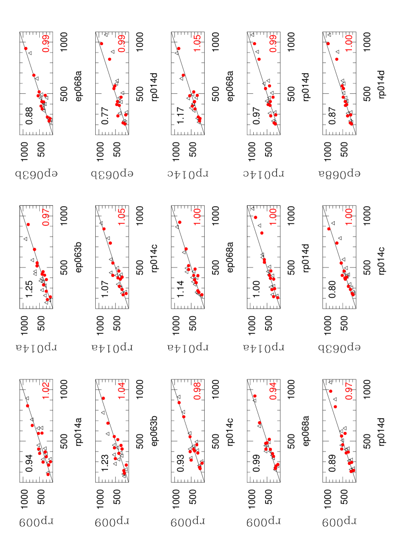
Figure 2: (To be seen in landscape) Measured flux of the 12 brightest sources at two different epochs for all the 15 possible combinations. Flux units are $\mu$Jy. The solid line is the equal flux line. Open triangles are the originally measured fluxes and the number at the top-left corner of each panel is the median of the ratios between the two epochs. Filled dots are the fluxes after the epoch-dependent correction listed in Table 5 are applied, and the number at the bottom-right corner of each panel is the median of the ratios between the two epochs.

2.4 Multi-epoch analysis

From the previous subsection we have derived an estimate of the noise error, $\sigma_{n}$, affecting our images and therefore our flux density measurements. In this subsection, we take full advantage of all the six epochs of observation to derive systematic scale offsets in the amplitudes of our images. To do so, we identified the 12 brightest objects detected at all epochs. Eleven of these sources (A0, A1, A2, A3, A4, A5, A7, A8, A10, A11, A12) have $\geq 5\sigma$ detections at all epochs with the remaining object (A15) detected with SNR $=4.5$ at one epoch, RP009, which is the observation with the highest noise. Then, for each of the 15 possible combinations of two different epochs, we plotted the measured flux at one epoch versus the measured flux at the other epoch for the 12 sources and all epochs. These ratios are shown in Fig. 2 as open triangles for all the 15 possible combinations The number in the top-left corner of each panel in Fig. 2 is the median of the ratio of the fluxes of the 12 sources. Clearly, variability adds scatter to the points with respect to the equal flux line, but we should roughly expect the same number of sources above and below this line, and therefore median values close to unity. This is clearly not the case, meaning that there are still some calibration issues at some of our epochs. These calibration offsets can be produced by errors in 1) the Tsys-based a-priori amplitude calibration, 2) the bandpass calibration, and/or 3) the transfer of amplitude corrections from the phase reference source to the target including possible coherence losses, as shown for example by Martí-Vidal et al., (2010). We applied epoch-dependent scale factors to the fluxes in order to minimize the deviation of the medians from unity. The derived scale factors are listed in Table 5 and the corrected fluxes are shown in Fig. 2 as filled dots. The number in the bottom-right corner of each panel in Fig. 2 is the median of the ratio of the fluxes of the 12 sources after the correction. We note that all the 12 sources used to derive the scale factors were already detected by Ulvestad, three years earlier than our observations. Therefore, it is highly unlikely that most of these sources are SNe which should display a monotonic decrease of the flux density. This is consistent with the fact that the derived scale factors do not show a monotonic trend with time that would signal a coherent decrease (or increase) in the flux densities of the 12 sources.

Table 5: Image scale factors

Date	Experiment	Scale Factor
	Code
08 Apr 2008	RP009	1.00
05 Dec 2008	RP014A	0.92
12 Jun 2009	EP063B	1.18
11 Dec 2009	RP014C	0.94
28 May 2010	EP068A	1.05
24 Nov 2010	RP014D	0.92

After applying these scale factors, the mean value of the 15 medians shown in the bottom-right corner of each panel in Fig. 2 is 1.000 with a dispersion of 0.029. Therefore, we take 2.9% as the residual calibration error, $\sigma_{cal}$, after the scale factors are applied.

3 Discussion

3.1 Comparison with previous observations

Here, we compare our results with those previously found by Pérez-Torres et al., (2009, henceforth PT09) and Ulvestad, (2009, henceforth U09). As already stated, PT09 reported on the first two epochs of observations (experiments RP009 and RP014A). 20/26 objects detected in PT09 are confirmed after 6 epochs by our average image, and only 6/26 are not confirmed by our new, more robust, selection criterion. These six sources were detected in only one epoch (RP014A) in PT09, and were among those with the faintest flux densities. Two of these sources (A16 and A24) have a $\simeq 4.5\sigma$ counterpart in the average image (peak flux of $83\leavevmode\nobreak\ \mu$Jy for both sources) and future observations might confirm they are real sources close to the detection threshold. The remaining four objects could have been spurious sources detected above the $5\sigma$ threshold because of a slight underestimate of the noise in the previous analysis, and are not confirmed by our new selection criteria, which are more robust against artifacts. On the other hand, one cannot simply rule out the possibility of sources which are detected in a single epoch, like A27 but at fainter flux density.

The comparison with the observations reported by U09 is also very interesting as those were done in the period around 2004-2005, three years before our first observations. U09 observed with the VLBA+GBT at both 2.3 GHz and 8.4 GHz, reaching an r.m.s. of about 20 $\mu$Jy/beam at both frequencies in his averaged images, which is a value very similar to the sensitivity in our averaged 5.0 GHz image. The 8.4 GHz observations are more appropriate for comparison purposes, since this observing frequency is closer to ours (5.0 GHz), and hence less affected by spectral effects, e.g. some sources could be affected by free-free absorption at frequencies around and below 2.3 GHz due to foreground H II regions, like in the case of A0 (Pérez-Torres et al., 2010). Twelve out of the 13 objects detected by U09 at 8.4 GHz are confirmed above $5\sigma$ and the remaining one has a $4\sigma$ counterpart in our average image. This implies that most of these sources are long-lived ($\!\!\!\phantom{\geq}\smash{\buildrel\over{\lower 2.67502pt\hbox{$\buildrel\lower 2.14001pt\hbox{$\displaystyle>$}\over{\sim}$}}}\,\,6$ years) objects.

On the other hand, there are eight sources detected in our 5.0 GHz observations that are not detected by U09 at neither frequency. These are A13, A14, A19, A25, A26, A27, A28 and A29. One source (A14) is the furthest from the image centre and might have not been detected by U09 for this reason. The remaining seven sources are among the weakest ones, but we note that there are equally weak sources (A18, A30 and A31) that were detected by U09.

While it is possible that image sensitivity and image reconstruction issues could account for the non-detection of some of the sources in the VLBA+GBT observations carried out in 2004-2005, we suggest that, for at least some of these objects, the most likely reason is the explosion of recent core-collapse SNe (CCSNe). While this point will be developed in detailed in Section 3.4. We note that sources A13, A19, A25 were suggested to be recently exploded SNe, and A14 a SNR by PT09, whereas sources A26 to A29 were not detected in those observations.

The 5.0 GHz radio luminosity of the compact objects in Arp 299-A covers almost an order of magnitude, (3–20)$\times 10^{26}$ erg s^-1 Hz^-1, with a median L${}_{\rm 5GHz}=6.9\times 10^{26}$ erg s^-1 Hz^-1 (we have excluded sources A1 and A5 since these are associated to the low luminosity AGN), and is systematically lower when compared with the mixed population of SNe and SNRs in Arp220 which have a median L${}_{\rm 5GHz}=60\times 10^{26}$ erg s^-1 Hz^-1 (Batejat et al., 2011). Unfortunately, luminosity by itself does not allow to discriminate between SNe and SNRs. Indeed, CCSNe can have a wide range of peak radio luminosities ($10^{25}-10^{29}$ erg s^-1 Hz^-1) depending on the wind properties (e.g. Alberdi et al., 2006; Romero-Cañizales et al., 2011). Our stacked image is sensitive to objects with a luminosity L${}_{\rm 5GHz}\geq 2.3\times 10^{26}$ erg s^-1 Hz^-1 (five times the r.m.s.), and thus allows the detection of sources with a steady, faint radio emission which would otherwise go undetected. Those sources must therefore be long-term emitters, i.e., relatively old CCSNe and/or SNRs. Our true sensitivity limit for detecting recently exploded SNe is given by the r.m.s. of each single epoch. From Table 4, the average r.m.s. is of $\simeq 33\,\mu$Jy/beam, our luminosity sensitivity for a threshold of $5\sigma$ is then L${}_{\rm 5GHz}\simeq 4.0\times 10^{26}$ erg s^-1 Hz^-1, implying that our observations are sensitive enough to allow the detection of at least some Type IIP SNe, which are known to be relatively faint radio emitters. We also note here that our 2.5-yr monitoring of Arp 299-A did not reveal a radio supernova similar, or brighter than A0, which exploded back in 2003, and most likely was a Type IIn event. This is unlike the case of Arp 220, where essentially every new detected radio supernova shows a radio power which is typical of Type IIn supernovae.

The radio emission from SNRs is expected to peak at the beginning of the Sedov phase (Huang et al., 1994), and the peak 5.0 GHz SNR luminosity can be roughly given by L${}_{\rm 5GHz}\approx 3.7\times 10^{24}(M_{ej1}/n_{\rm ISM})^{-0.53}$ erg s^-1 Hz^-1 (scaled to 5.0 GHz from Parra et al., 2007, assuming $\alpha=-0.7$). where $M_{ej1}$ is the ejecta mass in units of $10M_{\odot}$ and $n_{\rm ISM}$ is the interstellar medium (ISM) number density in cm^-3. The molecular number density in Arp 299-A is $n_{ISM}\sim 10^{4}$ (Aalto et al., 1997) and for $M_{ej1}=0.5$, we obtain a typical SNR 5.0 GHz luminosity of $7.0\times 10^{26}$ erg s^-1 Hz^-1 totally consistent with the median luminosity of the compact objects in Arp 299-A. Thus, the observed 5.0 GHz radio luminosities of the compact sources in Arp 299-A are in agreement with expectations from a population of relatively young CCSNe, SNRs, or a combination of both.

3.2 The variability and nature of the compact sources in Arp299-A

Variability can be an important tool to help classifying the compact sources in Arp 299-A as radio supernovae, supernova remnant, AGN or other more exotic classes of sources. For the sources in Table 3 with flux measurements $\geq 3\sigma$ at all six epochs, we calculated the chi-square:

$$\chi^{2}=\sum_{i=1}^{6}{S_{i}-\bar{S}\over\sigma_{\epsilon,i}^{2}}$$

where $\sigma_{\epsilon}=\sqrt{\sigma_{n}^{2}+\sigma_{cal}^{2}}$ is the combination of the noise error (see Sect. 2.3) and the residual calibration error (see Sect. 2.4) and $\bar{S}$ is the weighted average flux over the six epochs. We considered variable (V) the sources with a probability that the flux variations were due to random changes $p(\chi^{2})<1\%$, possibly variable (P) those with $1\%\leq p(\chi^{2})<5\%$ or otherwise non-variable (NV). The variability code is listed as last column in Table 3. The 19 sources for which this analysis was possible are evenly distributed in three categories: 7, variable, 5 probably variable and 7 not variable.

Figure 3 shows the derived light-curves for 5 variable sources and 5 non-variable sources. The time coverage is limited and the errors are relatively large, but nevertheless it is clear that some sources show significant variability and this variability has different characteristics. In the 2.5 years covered by our observations, we find sources which display a rather smooth increase and/or decrease in the flux density on a relatively long timescale (e.g. A0, A11 and A7 in the first two years) and sources with more erratic and faster variations (e.g. A2, A12 and the sharp increase in A7 on May 2010). Variability with similar characteristics has been observed also in the compact objects in Arp 220 (Rovilos et al., 2005).

Table 6: Variability and spectral index

Source	Var.Flag	$\alpha^{\mathrm{(a)}}$
A3	NV	$-0.46$
A4	NV	$-0.46$
A5	NV	$<-0.93$
A8	NV	$<-0.58$
A0	V	$>1.28$
A2	V	$-0.21$
A7	V	$0.07$
A11	V	$-0.14$
A12	V	$-0.22$

• Spectral index calculated between 2.3 and 8.4 GHz from Ulvestad, (2009) with the exception of A0 where $\alpha$ is between 1.7 and 5.0 GHz from Pérez-Torres et al., (2010).

We also note that four sources classified as non-variable (NV) and five classified as variable (V) have a two-point spectral index measured between 2.3 and 8.4 GHz, or an upper/lower limit in U09. The values are listed in Table 6, where $\alpha$ is defined as $S_{\nu}\propto\nu^{\alpha}$.

Coincidentally, there is a correlation between the radio spectral index measured between 2.3 and 8.4 GHz observations carried out around 2004-2005 and the flux density variability at 5.0 GHz in the period 2008-2010. The non-variable sources have steep spectral index ($\!\!\!\phantom{\leq}\smash{\buildrel\over{\lower 2.67502pt\hbox{$\buildrel\lower 2.14001pt\hbox{$\displaystyle<$}\over{\sim}$}}}\,\,-0.5$), while the variable sources have flat, or inverted, spectral index ($\!\!\!\phantom{\geq}\smash{\buildrel\over{\lower 2.67502pt\hbox{$\buildrel\lower 2.14001pt\hbox{$\displaystyle>$}\over{\sim}$}}}\,\,-0.2$). Source A5 has been already identified with a bright knot/hot-spot component in the A1-A5 complex by Pérez-Torres et al., (2010), where A1 was identified with the low luminosity AGN in Arp 299-A. The steep spectrum and lack of variability are consistent with this hypothesis. For the remaining three sources, their steep radio spectra and lack of significant variability are strong indicators that the sources are likely SNRs passively evolving in the interstellar medium.

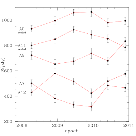
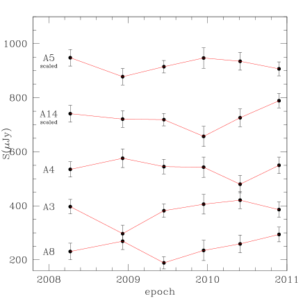
Figure 3: Upper panel: light curves for 5 sources classified as variable. The data for source A11 and A0 have been scaled up by 500 $\mu$Jy and 600 $\mu$Jy respectively to avoid confusion. Lower panel: light curves for 5 sources classified as non-variable. The data for A14 and A5 have been scaled up by 500 $\mu$Jy and 700 $\mu$Jy respectively to avoid confusion.

On the other hand, all objects showing significant variability for which the previous observations allowed to derive a spectral index, have flat or inverted radio spectra. The identification of the nature of these sources is more complex. The radio light-curve of SNe is determined by the competition between decaying synchrotron emission and decreasing free-free absorption, producing radio peaks that occur progressively later at longer wavelenghts (Weiler et al., 2002). Such a radio light curve evolution yields also to spectral indices, which evolve from inverted to flat –during their optically thick phase, while the supernova is its way to the peak flux density– and then become steep, once the supernova is in its optically thin phase for all the compared frequencies, well past the peak. None of our sources is neither fading away monotonically, nor rising and falling coherently as it would be expected from a SN. After a rise to a maximum, the flux density of a radio SN generally declines, although in some case it is known to fluctuate because of inhomogeneities in the supernova circumstellar environment (Weiler et al., 2002; Montes et al., 2000). All our variable sources show both increase and decrease of the radio flux density in the period, about 2.5 years, covered by our monitoring. Only one of them, A0, has been clearly identified with a radio SN that reached its maximum around 2003 (Neff et al., 2004; Ulvestad, 2009; Pérez-Torres et al., 2009). The smooth variability in A0 during the period of our monitoring could be an example of the fluctuations observed during the decaying phase in other SNe (Weiler et al., 2002; Montes et al., 2000).

Most compact objects in Arp 220 are classified either as SNe or as SNRs (Parra et al., 2007). However, recent multi-wavelength observations have shown evidence for some objects being in a transition phase, from SN to SNR (Batejat et al., 2011). This could easily be the case for some of the objects in Arp 299-A as well. For example, the source labelled as A7 (see Fig.3) displays a steady decay of flux density for at least two years, followed by a fast ($\sim 0.5$ yr) and strong brightening ($50\%$ of flux density increase) which is suggestive of A7 experiencing a transition from SN to SNR. Those ’bursts’ in flux density would be produced by the impact of the freely expanding forward supernova shock into the ISM.

Our VLBI monitoring at 5.0 GHz is continuing and we are confident that the forecoming observations, together with the spectral indices for a larger number of sources derived from simultaneous 1.4 and 5.0 GHz observations, will allow to shed more light on the variability-spectral index relationship suggested by Table 6.

3.3 Extended and compact emission in Arp 299-A

Figure 4: MERLIN image at 5.0 GHz with a resolution of 46 $\times$ 44 mas at position angle -75^∘. The beam is shown at the bottom-right corner. Contours levels are a geometric progression in square root of 2, starting from 5 times the off-source r.m.s of 64 $\mu$Jy/beam. The position of the 26 compact radio sources detected by our EVN observations are shown with crosses or diamonds (A1 and A5)

We show in Fig. 4 the contours of the MERLIN image at 5.0 GHz with a resolution of $46\times 44$ mas. The position of the 26 compact radio sources detected by our EVN observations are shown with crosses or diamonds. The MERLIN data on Arp 299 were obtained in the course of a Target of Opportunity observation aimed at searching for radio emission from supernovae 2010O and 2010P, which resulted in upper limits to their radio emission (Beswick et al. 2010). The EVN is essentially sensitive to very compact emission, while MERLIN is also sensitive to the more diffuse emission between the compact components and has a resolution of $46\times 44$ mas. The flux density detected in compact sources above $5\sigma$, as imaged with the EVN, is on average $\simeq$ 7.3 mJy. This compact flux is spread over an area of $\approx 0.71\times 0.68$ arcsec² ($\simeq 154\times 148$ pc²). The total flux detected above $5\sigma$ in the MERLIN image is $\simeq 97\pm 10$ mJy over an area of $\approx 0.77\times 0.52$ arcsec², essentially the same area covered by the compact sources in our EVN observations. The MERLIN flux is consistent with the flux ($101.1\pm 5.0$ mJy) measured by Neff et al., (2004) from VLA observations at 5.0 GHz with a resolution of $0.38\times 0.31$ arcsec. From Neff et al., (2004), it is possible to derive a spectral index $\alpha\simeq-0.5$ between 4.9 and 8.4 GHz for a region fitted with a Gaussian FWHM of $0.38\times 0.30$ arcsec in P.A. $127^{\circ}$, which is consistent with the size of the MERLIN detected extended emission.

The MERLIN emission is dominated by diffuse flux, as the EVN-detected compact sources sum up to $<10\%$ of the total emission detected in our MERLIN image. The radio spectral index of $\alpha\simeq-0.5$ implies that the extended radio emission in the MERLIN image is synchrotron emission from relativistic electrons, the bulk of which are originally produced in young SNe and SNRs, since the AGN in Arp 299-A contributes very little (Pérez-Torres et al., 2010) . Here, we notice three aspects. First, the compact sources and the extended emission trace the same physical region. As expected, the brightest patch of diffuse emission coincides with the region of highest density of compact sources, but some compact sources are found right at the edges of the diffuse emission as well. The extended emission has a 5.0 GHz luminosity $L=2.3\times 10^{29}$ erg s^-1 Hz^-1. Since this radio emission must be produced by young SNe and SNRs, the inferred core-collapse supernova rate, using the standard relation in Condon, (1992), is $\nu_{\rm SN}\simeq 0.40-0.65$ SN/yr for $\alpha$ between $-0.5$ and $-0.8$. This value is consistent with the estimate $\nu_{\rm SN}\simeq 0.7$ SN/yr based on the fraction of far-infrared luminosity attributed to Arp 299-A (Alonso-Herrero et al., 2000, 2009; Romero-Cañizales et al., 2011), and indicates that the main bulk of the (recent) star formation in Arp 299-A is most likely happening in its central $\sim$150 pc.

Second, the radiation density in the nuclear region of Arp 299-A is so large as to make Inverse Compton (IC) losses exceed those by synchrotron radiation. In fact, since the energy source, or sources, powering the radio emission cannot be larger than the observed radio source size, the radiation energy density $u_{\rm r}$ at the surface of a spherical radio component covering a solid angle $\Omega$ must be at least

$$u_{\rm r}\geq\frac{4\,\pi}{c}\left(\frac{\rm L_{ir}}{\Omega\,D^{2}}\right)$$

. The solid angle covered by the diffuse (MERLIN) radio emission is $\Omega\approx 0.48$ arcsec². We first estimated the 1.4 GHz radio emission from the total 5.0 GHz flux density measured by MERLIN ($\sim$97 mJy) converted to 1.4 GHz assuming the spectral index, $\alpha\simeq-0.5$. Then, we obtained the corresponding FIR luminosity for this region, $L_{\rm IR}\approx 4.8\times 10^{10}L_{\odot}$, using the standard FIR-to-radio relation (e.g. Yun et al. (2001)). The radiation density is $u_{\rm r}\!\!\!\phantom{\geq}\smash{\buildrel\over{\lower 2.67502pt\hbox{$\buildrel\lower 2.14001pt\hbox{$\displaystyle>$}\over{\sim}$}}}\,\,3.5\times 10^{-7}$  erg cm^-3. Since the magnetic energy density is $B^{2}/(8\,\pi)$, the magnetic field would have to be at least $B\!\!\!\phantom{\geq}\smash{\buildrel\over{\lower 2.67502pt\hbox{$\buildrel\lower 2.14001pt\hbox{$\displaystyle>$}\over{\sim}$}}}\,\,3$ mG to overcome IC losses. However, the equipartition magnetic field corresponding to the diffuse synchrotron radio emission traced by MERLIN is $B_{\rm eq}\simeq 160\,\mu$G (here, we assumed a cosmic ray protron/electron energy ratio of 100 and unity filling factor), which is a very similar value obtained for the central 200 pc of the ULIRG IRAS 23365+3604 (Romero-Cañizales et al., 2012). Therefore, unless strong deviations from equipartition exist, IC losses will dominate over synchrotron losses in the central $\sim$150 pc-region of Arp 299-A. Thus, the lifetimes of the relativistic electrons responsible for the 5.0 GHz emission, which in an equipartition magnetic field would be of $\sim 2.3\times 10^{5}$ yr, are heavily cut down to $\!\!\!\phantom{\leq}\smash{\buildrel\over{\lower 2.67502pt\hbox{$\buildrel\lower 2.14001pt\hbox{$\displaystyle<$}\over{\sim}$}}}\,\,$2900 yr due to IC losses. This requires that the relativistic electrons responsible for synchrotron emission in the central $\sim$150 pc of Arp 299-A are being continuously reaccelerated or, alternativelty, that there is a continuous injection of fresh relativistic electrons. The natural places for such acceleration would be the shocks of the SNe and SNRs that our EVN image reveals as strong synchrotron radio emitters.

Third, we note that four of the six sources classified as non-variable SNe/SNRs (A3, A8, A14 and A29) lie at the outskirts of the diffuse, extended emission traced by our MERLIN image in Fig. 4 and consequently at the edge of the nuclear starburst region. This may indicate that all those objects are SNRs, and that the transition from SN to SNR may happen faster in the outskirst of the nuclear region of Arp 299-A, where the densities are not expected to be so extreme as in the inner few pc, where intense activity is happening in scales of a few years (e.g., A0, A27). The non-detection of A0 at low frequencies, even several years after its explosion (Pérez-Torres et al., 2010), suggests that H II regions (and consequently free-free absorption) are likely more frequent in the central region of Arp 299-A, which would be in agreement with the above scenario. On the contrary, A14 and A29, which were not detected by U09 in his very sensitive observations, could be examples of particularly fast evolving objects, that would be currently transitioning to SNRs.

3.4 New CCSNe and the CCSN rate of Arp 299-A

Figure 5: Zoom of the central region around component A1 observed during experiment RP014C. The beam is shown in the bottom right corner and the resolution is $10\times 8$ mas. Contours are drawn at levels -5, 5, 6, 7, 10, 15, 20, 40 times the r.m.s. noise listed in Table 1. The compact source A27 is detected with $SNR=7$

As previously mentioned, in the period monitored by our observations none of the compact sources in Arp 299-A shows a monotonically decreasing flux density which could be interpreted as the optically thin, decaying phase of a CCSN. The best chance to identify new SNe is to look for objects without a counterpart in the earlier U09 observations. As already said at the end of Sec. 2.2, there are 8 sources detected by the present observations at 5.0 GHz, and not detected by U09 at neither 2.3, nor 8.0 GHz.

Based on the far-infrared luminosity $L_{\rm FIR}=2.7\times 10^{11}$ erg s^-1 for Arp 299-A (Charmandaris et al., 2002), and assuming the CCSN rate for Arp 299-A is $\nu_{\rm SN}\simeq 0.72$ SN/yr (Alonso-Herrero et al., 2000; Romero-Cañizales et al., 2011) the expected number of CCSNe that should have exploded in the $\sim$5.3 years elapsed between the VLBA+GBT observations and our latest EVN observation is $\sim$3.7. Since the explosion of SNe is an intrinsically stochastic phenomenon where Poisson statistics applies, we should actually expect that the number of new supernovae be in the range [1.9, 5.6] where the range corresponds to 1$\sigma$ confidence level (Gehrels, 1986).

Based on the 5.0 GHz radio light-curve behaviour displayed by the sources above, there seems to be clear evidence for at least two objects being newly exploded supernovae in the 2.5-yr period covered by our observations, namely A25 and A27. A25 was already suggested to be a new SN by PT09, and its behaviour supports a scenario where it reached its peak luminosity around 2008.9 (+/- 0.3 yr) and started to slowly decline afterwards. The luminosity at the measured peak flux density is $6.7\times 10^{26}$ erg s^-1 Hz^-1. Its behaviour and peak luminosity is consistent with a type II supernova, most likely a type IIP, or type IIL, based on its relatively modest luminosity peak and its slow evolution. A27 is detected, with SNR = 7, in just one epoch on December 2009 (see Fig. 5), but is undetected at all other epochs. The corresponding peak luminosity is L${}_{\rm 5GHz}=6.2\times 10^{26}$ erg s^-1 Hz^-1. A search for possible counterparts at other epochs within a circular region with a radius of 5 pixels centered on the source’s peak failed to find emission above a $3\sigma$ threshold. We have challenged the reliability of A27, imaging the data set with different resolutions using different weighting schemes and we have always detected the radio source with an uncertainty on its position less than 1 pixel (0.5 mas). Since the image size is $2048\times 2048$ pixels the probability of detecting a spurious $7\sigma$ spike of (Gaussian) noise in the total image area is $<10^{-5}$. This probability would be even smaller, if we considered only the restricted area covered by the detected sources. Therefore, even if detected at just one single epoch, we are confident that A27 is a real source. Its flux density rise and decay are fast. At the previous and following epochs, 6 months earlier and later, we have upper limits of 78 $\mu$Jy and 75 $\mu$Jy, respectively. Such a fast rise and decay of the flux strongly suggests that A27 was a Type Ib/c supernova.

Since each of our individual observations has a typical r.m.s of $\!\!\!\phantom{\geq}\smash{\buildrel\over{\lower 2.67502pt\hbox{$\buildrel\lower 2.14001pt\hbox{$\displaystyle>$}\over{\sim}$}}}\,\,30\mu$Jy, which corresponds to a 5.0 GHz luminosity $\simeq 1.0\times 10^{26}$ erg s^-1, we are sensitive to modest radio emitting supernovae, including Type IIP SNe, but not to very faint radio supernovae. At any rate, our firm discovery of at least two CCSNe in our 2.5 yr monitoring corresponds to a lower limit of 0.8 SN/yr for the CCSN rate in the nuclear starburst in Arp 299-A. Taking into account Poisson statistics, our measured value of the CCSN rate, with errors bars corresponding to 1$\sigma$ errors, is $\nu_{\rm SN}\!\!\!\phantom{\geq}\smash{\buildrel\over{\lower 2.67502pt\hbox{$\buildrel\lower 2.14001pt\hbox{$\displaystyle>$}\over{\sim}$}}}\,\,0.80^{+1.06}_{-0.52}$ SN/yr. This is the first direct determination of the core-collapse supernova rate in Arp 299-A ever, and while it agrees with previous estimates, it represents a lower limit to the true CCSN rate of Arp 299-A. A more accurate and reliable determination of the CCSN rate for Arp 299-A will necessarily require a longer monitoring to overcome Poisson statistics.

We emphasize the fact that this value of $\nu_{\rm SN}$ is a lower limit to the true core-collapse supernova rate of the Arp 299-A system. Indeed, if we take into account SN2010O, which exploded in Arp 299-A (although far from its nuclear region, at a distance of $\simeq$1.4 kpc), during the time covered by our obsevations, the overall CCSN rate for the galaxy would then be $\nu_{\rm SN}\simeq 1.20^{+0.77}_{-0.43}$ SN/yr. If confirmed by future observations, this value would imply a larger CCSN rate than expected from empirical conversions of far-infrared luminosity into CCSN rates.

We also remark here that A27 exploded at a mere 7.2 pc from A0, the only other source that has been unambiguously identified with a SN, and at 7.9 pc from the AGN in Arp 299-A. The detection of two CCSNe in less than 10 years exploding at a (projected) distance of $\!\!\!\phantom{\leq}\smash{\buildrel\over{\lower 2.67502pt\hbox{$\buildrel\lower 2.14001pt\hbox{$\displaystyle<$}\over{\sim}$}}}\,\,$7 pc apart could suggest that A0 and A27 were part of a super-star cluster (SSC), hosting large numbers of massive stars in the central region of Arp 299-A. SSCs seen in the optical and near-infrared in other merging galaxies have typical radii $\sim 4$ pc but, in particular young SSCs (ages less than 10 Myr), may be as large as tens of parsecs (Whitmore et al., 1999). Near-infrared Lai et al., (1999) and optical (Alonso-Herrero et al., 2000) observations have indeed detected young SSCs in the central regions of Arp 299. A0 was a very bright, long-lasting radio supernova, implying it must have probably been a Type IIn SN. A27 was also relatively brigth, but its fast evolution indicates that it is most likely a Type Ib/c event. Both A0 and A27 must then have had massive ($M\simeq 18-35M_{\odot}$) progenitors, whose lifetimes are $\!\!\!\phantom{\leq}\smash{\buildrel\over{\lower 2.67502pt\hbox{$\buildrel\lower 2.14001pt\hbox{$\displaystyle<$}\over{\sim}$}}}\,\,$ 10 Myr. Evolutionary models for the radio emission in starbursts by Perez-Olea & Colina (1995) show that the SN rate in an instantaneous burst (for a Salpeter IMF with lower and upper limits of 0.85 and 120 M_⊙, respectively) are in the range (6-11)$\times 10^{-10}$ yr^-1M_⊙^-1 for a cluster in the time interval between 3-10 Myr. Since SSCs in galaxies outside the local group and with ages $\!\!\!\phantom{\leq}\smash{\buildrel\over{\lower 2.67502pt\hbox{$\buildrel\lower 2.14001pt\hbox{$\displaystyle<$}\over{\sim}$}}}\,\,$ 10 Myr have at most $M\sim 5\times 10^{6}$ M_⊙(Portegies Zwart et al. 2010), the CCSN rate for a SSC of $5\times 10^{6}$ M_⊙would then be $\sim 0.0030-0.0055$ yr^-1, or at most 1 SN every 181 yr. The (Poisson) probability of having more than 1 CCSN in such a SSC after just $\sim 6.5$ yr is $6.2\times 10^{-4}$. We therefore rule out the possibility that both A0 and A27 exploded in the same SSC, and suggest instead that these CCSNe exploded in two different SSCs of smaller sizes. The two SSCs could be intrinsically close or appear nearby due to projection effects.

In addition, four other sources (A13, A19, A26, A29) have radio light curves in agreement with them being slowly evolving SNe, similarly to the case of A0, but the weakness of these sources and the limited number of epochs prevents a definite conclusion. We defer the classification of these objects to another paper, where spectral information and additional new observing epochs would allow us to type them more securely. Yet, we stress here that our main result (the discovery of at least two new SNe) implies a CCSN rate for Arp 299-A of $\nu_{\rm SN}\!\!\!\phantom{\geq}\smash{\buildrel\over{\lower 2.67502pt\hbox{$\buildrel\lower 2.14001pt\hbox{$\displaystyle>$}\over{\sim}$}}}\,\,0.80$ SN/yr, and suggests that most star formation is currently occurring in the central $\simeq$150 pc of Arp 299-A.

3.5 Other transient sources

In Table 3, we reported on the variability of the compact sources in Arp 299-A based on a $\chi$-squared test. This test was applied to those sources whose peak of brightness was above 3 times the noise at all epochs. Such a requirement was adopted in order to maximize the number of points in the radio light-curves and therefore better constrain the variability behaviour, but it fails to account for the possible existence of fast-varying objects (e.g., rapidly evolving type Ib/c SNe or other transient sources) that are not detected at one or more epochs.

Here, we discuss the nature of some of the sources that, while not fulfilling the criterium for the variability analysis, show significant variability albeit of a less extent. In particular, PT09 already discussed the possibility that source A6 was a microquasar (e.g. Mirabel & Rodriguez, 1994), based on its radio luminosity, radio behaviour at 5.0 GHz, and proximity to two X-ray sources. Now, from our six epochs of observation, and from its radio longevity and spectrum (it was already reported at 2.3 Ghz by U09, but not at 8.4 GHz, implying $\alpha\!\!\!\phantom{\leq}\smash{\buildrel\over{\lower 2.67502pt\hbox{$\buildrel\lower 2.14001pt\hbox{$\displaystyle<$}\over{\sim}$}}}\,\,-1.03$ between 2.3 and 8.4 GHz), we suggest that A6 is a microquasar which flashes on and off. A similar behaviour to that of A6 is displayed by A28. In fact, the source seems to show epoch-to-epoch (i.e., approximately every six-months) flux density variations of $\sim$40%, or even higher. Since A28 was not detected by U09 in his 2004-2005 observations, this implies that it is a young source ($t\!\!\!\phantom{\leq}\smash{\buildrel\over{\lower 2.67502pt\hbox{$\buildrel\lower 2.14001pt\hbox{$\displaystyle<$}\over{\sim}$}}}\,\,7$ yr). While it is possible that A28 could be also another microquasar, we cannot exclude that it is a different object, even a radio supernovae since, as we mentioned above, non-standard SNe seem to be relatively normal in starburst galaxies (Rovilos et al., 2005).

Nonetheless, we defer a definitive classification of those sources to a separate publication, where contemporaneous spectral information will be discussed.

4 Summary

We have monitored the nearby LIRG Arp 299-A at 5.0 GHz for 6 epochs with the European VLBI Network. The observations have been carried out once every 6 months for a period of 2.5 years. The main results of these observations are as follows.

1. Twenty-five compact sources are detected above the $5\sigma$ detection threshold in the 6-epoch average image. One more source, even if below the detection threshold in the average image is detected with high confidence (SNR=7) at a single epoch and is considered as a real fast varying source, probably a type Ib/c SN. Two sources (A1 and A5) have been already identified as components of a low-luminosity AGN in Arp 299-A (Pérez-Torres et al., 2010). The 26 detections occupy a region with a diameter of about 150 pc.

2. Comparison with previous observations shows that most of the compact sources have been already detected at 2.3 and/or 8.4 GHz in earlier VLBA+GBT observations with comparable sensitivity (Ulvestad, 2009). Only eight sources appear to be objects not reported in U09. Some of these new detections might be due to a slightly larger area imaged by our observations, but we are confident that some of them are recently exploded CCSNe.

3. The 5.0 GHz radio luminosities of the compact objects in Arp 299-A are in the range $3-20\times 10^{26}$ erg s^-1 Hz^-1 with a median of $6.9\times 10^{26}$ erg s^-1 Hz^-1 (A1 and A5 have been excluded since part of a low-luminosity AGN) about an order of magnitude lower than the median luminosity of the population of SNe/SNRs found in Arp 220 (Batejat et al., 2011), which suggests that the population of exploding SNe in Arp 299-A might be characterized by a different IMF. A longer monitoring of the compact sources in the nuclear region of Arp 299-A should allow us to unambiguously answer this relevant question. Since the observed radio luminosities are also consistent with typical SNR luminosities at the beginning of the Sedov phase, we conclude that the 5.0 GHz observed luminosity are in agreement with expectations from a population of relatively young CCSNe, or SNRs, or a combination of both.

4. We have quantified the variability over the 6 epochs (2.5 years) for the 19 sources that were detected at all epochs. The sources are evenly distributed in the variable, probably variable and non-variable classes. Variable sources can show complex radio light curves which are difficult to interpret. Using spectral index information from the literature we find that sources classified as variable have flatter radio spectra ($\alpha\!\!\!\phantom{\geq}\smash{\buildrel\over{\lower 2.67502pt\hbox{$\buildrel\lower 2.14001pt\hbox{$\displaystyle>$}\over{\sim}$}}}\,\,-0.2$) than non-variable sources ($\alpha\!\!\!\phantom{\leq}\smash{\buildrel\over{\lower 2.67502pt\hbox{$\buildrel\lower 2.14001pt\hbox{$\displaystyle<$}\over{\sim}$}}}\,\,-0.5$). The non-variable and steep spectrum sources could be associated to SNRs passively evolving in the ISM. More complex is the identification of the variable flat-spectrum sources which might contain SNe and objects in a transition phase from SN to SNR. A longer monitoring to better characterize the variability properties together with radio spectral index derived from simultaneous observations (Pérez-Torres et al. in preparation) are necessary to confirm these hypothesis.

5. A MERLIN image at 5.0 GHz with a resolution of $46\times 44$ mas shows diffuse, extended emission cospatial with the distribution of the compact sources. The extended emission is non-thermal ($\alpha\simeq-0.5$) and can be explained with synchrotron emission from relativistic electrons originally produced in SNRs. The luminosity of the extended emission implies a supernovae rate of $\simeq 0.40-0.65$ SN/yr, which is consistent with that derived from the far-infrared luminosity of Arp 299-A, and also in marginal agreement with our direct estimate from the new discovered SNe.

6. We find clear evidence for two recently exploded CCSNe in Arp 299-A. The object labelled as A25 has reached a maximum around epoch 2008.9 ($\pm 0.3$ yr) and started to slowly decline afterwards. The peak luminosity and the relatively slow declining phase suggest that A25 is most likely a type II CCSN. The object labelled as A27 was detected with relatively high confidence (250 $\mu$Jy with SNR=7) at a single epoch. Six months later we have an upper limit of 75 $\mu$Jy. Since the probability of a fake 7$\sigma$ detection over the image area is $<10^{-5}$, we interpret A27 as a fast evolving type Ib/c supernova. From those two CCSNe, we obtain a CCSN rate for the innermost $\sim$150 pc of Arp 299-A of $\nu_{\rm SN}\simeq$0.80 SN/yr, which is in broad agreement with previous estimates at much poorer resolution and which is also supported by our CCSN estimate obtained from the diffuse, non-thermal radio emission traced by our MERLIN observations. This result strongly hints at the bulk of the current star formation taking place in the central $\sim$150 pc of Arp 299-A.

   This value represents also a lower limit to the true core-collapse supernova rate of the whole Arp 299-A system. If we consider also SN2010O, which exploded also in Arp 299-A (although at a distance of $\simeq$1.4 kpc from the nuclear region) the overall CCSN rate for the Arp 299-A galaxy is $\nu_{\rm SN}\simeq 1.20^{+0.77}_{-0.43}$ SN/yr, which would imply a larger CCSN rate than expected from empirical conversions of far-infrared luminosity into CCSN rates.

7. Finally, we note that a few objects that were excluded from the variability analysis because they were undetected ($<3\sigma$) in at least one epoch show peculiar epoch-to-epoch flux density variations of up to 40% or larger (e.g. A6 and A28). These radio sources could be associated to microquasars or peculiar SNe, and further multifrequency observations are necessary for a proper classification.