EVALUATING SOURCES OF VARIABILITY IN PATHWAY PROFILING

Abstract

1 Motivation:

A bioinformatics platform is introduced aimed at identifying models of disease-specific pathways, as well as a set of network measures that can quantify changes in terms of global structure or single link disruptions.The approach integrates a network comparison framework with machine learning molecular profiling. The platform includes different tools combined in one Open Source pipeline, supporting reproducibility of the analysis. We describe here the computational pipeline and explore the main sources of variability that can affect the results, namely the classifier, the feature ranking/selection algorithm, the enrichment procedure, the inference method and the networks comparison function.

2 Results:

The proposed pipeline is tested on a microarray dataset of late stage Parkinsons’ Disease patients together with healty controls. Choosing different machine learning approaches we get low pathway profiling overlapping in terms of common enriched elements. Nevertheless, they identify different but equally meaningful biological aspects of the same process, suggesting the integration of information across different methods as the best overall strategy.

3 Availability:

All the elements of the proposed pipeline are available as Open Source Software: availability details are provided in the main text.

4 Contact:

annalisa.barla@unige.itannalisa.barla@unige.it

5 Introduction

We present a computational framework for the study of reproducibility in network medicine studies (Barabasi et al., 2011). Networks, molecular pathways in particular, are increasingly looked at as a better organized and more rich version of gene signatures. However, high variability can be injected by the different methods that are typically used in system biology to define a cellular wiring diagram at diverse levels of organization, from transcriptomics to signalling, of the functional design. For example, to identify the link between changes in graph structures and disease, we choose and combine in a workflow a classifier, the feature ranking/selection algorithm, the enrichment procedure, the inference method and the networks comparison function. Each of these components is a potential source of variability, as shown in the case of biomarkers from microarrays (The MAQC Consortium, 2010). Considerable efforts have been directed to tackle the problem of poor reproducibility of biomarker signatures derived from high-throughput -omics data (The MAQC Consortium, 2010), addressing the issues of selection bias (Ambroise and McLachlan, 2002; Furlanello et al., 2003) and more recently of pervasive batch effects (Leek et al., 2010). We argue that it is now urgent to adopt a similar approach for network medicine studies. Stability (and thus reproducibility) in this class of studies is still an open problem (Baralla et al., 2009). Underdeterminacy is a major issue (De Smet and Marchal, 2010), as the ratio between network dimension (number of nodes) and the number of available measurements to infer interactions plays a key role for the stability of the reconstructed structure. Furthermore, the most interesting applications are based on inferring networks topology and wiring from high-throughput noisy measurements (He et al., 2009).

Despite its common use even in biological contexts (Sharan and Ideker, 2006), the problem of quantitatively comparing networks (e.g., using a metric instead of evaluating network properties) is a still an open issue in many scientific disciplines. The central problem is of course which network metrics should be used to evaluate stability, whether focusing on local changes or global structural changes. As discussed in Jurman et al. (2011), the classic distances in the edit family focus only on the portions of the network interested by the differences in the presence/absence of matching links. Spectral distances - based on the list of eigenvalues of the Laplacian matrix of the underlying graph - are instead particularly effective for studying global structures. In particular, the Ipsen-Mikhailov (Ipsen and Mikhailov, 2002) distance was found robust in a wide range of situations (Jurman et al., 2011). However, global distances can be tricked by isomorph or close to isomorph graphs. In Jurman et al. (2012), both approaches are improved by proposing a glocal measure which combines a spectral distance with a typical Hamming local editing component. In this paper we use this new tool to quantify how stability of network reconstruction is modified in practice by the different inference and enrichment methods.

Pathway enrichment methods are widely used in bioinformatics analysis, for example to assess the relevance of biomarker lists or as a first step in network analysis. The enrichment step is performed using the functional information stored in the Kyoto Encyclopedia of Genes and Genomes (KEGG) database (Kanehisa and Goto, 2000) and in the Gene Ontology (GO) database (Ashburner et al., 2000). The reconstruction of molecular pathways from high-throughput data is then based on the theory of complex networks (e.g. Strogatz (2001); Newman (2003); Boccaletti et al. (2006); Newman (2010); Buchanan et al. (2010)) and, in particular, in the reconstruction algorithms for inferring networks topology and wiring from data (He et al., 2009).

The stability analysis is applied to networks identifying common and specific network substructures that could be basically associated to disease. The overall goal of the pipeline is to identify and rank the pathways reflecting major changes between two conditions, or during a disease evolution. We start from a profiling phase based on classifiers and feature selection modules organized in terms of experimental procedure by Data Analysis Protocol (The MAQC Consortium, 2010), obtaining a ranked list of genes with the highest discriminative power. Classification tasks as well as quantitative phenotype targets can be considered by using different machine learning methods in this first phase. Alternative methods are made available as components of one Open Source pipeline system. The problem of underdeterminacy in the inference procedure is avoided by focusing only on subnetworks, and the relevance of the studied pathways for the disease is judged in terms of discriminative relevance for the underlying classification problem.

As a testbed for the glocal stability analysis, we compare network structures on a collection of microarray data for patients affected by Parkinson’s disease (PD), together with a cohort of controls (Zhang et al., 2005b). PD is a neurodegenerative disorder that impairs the motor skills at the onset and the cognitive and the speech functions successively. The goal of this task is to identify the most relevant dirsupted pathways and genes in late stage PD. On this dataset, we show that choosing different profiling approaches we get low overlapping in terms of common enriched pathways found. Despite this variability, if we consider the most disrupted pathways, their glocal distances (between case and control networks) share a common distribution assessing equal meaningfulness to pathways found starting from different approaches.

6 Materials and Methods

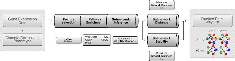
Figure 1: General scheme of the analysis pipeline, with the indication of the algorithms and tools used in the PD dataset application (lower boxes).

The machine learning pipeline adopted in this paper has been originally introduced in (Barla et al., 2011). As shown in Figure 1, it handles case/control transcription data through four main steps, from a profiling task to the identification of discriminant pathways. The pipeline is independent from the algorithms used: here we describe each step and the implementation adopted for the following experiments evaluating the impact of different enrichment methods in pathway profiling.

Formally, we are given a collection of $n$ subjects, each described by a $p$-dimensional vector $x$ of measurements. Each sample is also associated with a phenotypical label, e.g. $y\!=\!\{1,-1\}$, assigning it to a class (in a classification task). The dataset is therefore represented by a $n\!\times\!p$ expression data matrix $X$, where $p\!\gg\!n$, and a corresponding labels vector $Y$.

Feature Selection Step
The matrix $X$ is used to feed the profiling part of the pipeline within a proper Data Analysis Protocol, which will ensure accurate and reproducible results (The MAQC Consortium, 2010). The prediction model $\mathcal{M}$ is built by using two different algorithms for classification and feature ranking. The more recent one is the $\ell_{1}\ell_{2}$ regularization with double optimization, capable of selecting subsets of discriminative genes. The algorithm can be tuned to give a minimal set of discriminative genes or larger sets including correlated genes and it is based on the optimization principle presented in Zou and Hastie (2005). The implementation used consists of two stages (De Mol et al., 2009) and it is cast in nested loops of $10$-fold cross-validation (Barla et al., 2008). The first stage identifies the minimal set of relevant variables (in terms of prediction error), while, starting from the minimal list, the second one selects the family of (almost completely) nested lists of relevant variables for increasing values of linear correlation. As alternative choice we consider Liblinear, a linear Support Vector Machine (SVM) classifier specifically designed for large datasets (millions of instances and features) (Fan et al., 2008). In particular, the classical dual optimization problem with L2-SVM loss function is solved with a coordinate descent method. For our experiment we adopt the $\ell_{2}$-regularized penalty term and the module of the weights for ranking purposes within a $100\times 3$-fold cross validation schema. We build a model for increasing feature sublists where the feature ranking is defined according to the importance for the classifier. We choose the model, and thus the top ranked features, providing a balance between the accuracy of the classifier and the stability of the signature (The MAQC Consortium, 2010). Thus, the output of this first step is a gene signature $g_{1},...,g_{k}$ (one for each model $\mathcal{M}$) containing the $k$ most discriminant features, ranked according their frequency score.

Pathway Enrichment
The successive enrichment phase derives a list of relevant pathways from the discriminant features, moving the focus of the analysis from single genes to functionally related pathways. As outlined in the review by Huang et al. (2009), in the last 10 years the gene-annotation enrichment analysis field has been growing rapidly and several bioinformatics tools have been designed for this task. Huang et al. (2009) provide a unique categorization of these enrichment tools in three major categories based on the underlying algorithm: singular enrichment analysis (SEA), gene set enrichment analysis (GSEA), and modular enrichment analysis (MEA). We choose one representative $\mathcal{E}$ for each class for our comparison referring as sources of information $\mathcal{D}$ both to the KEGG, to explore known information on molecular interaction networks, and GO, to explore functional characterization and biological annotation. In the first category we choose WebGestalt (WG), an online gene set analysis toolkit (Zhang et al., 2005a) taking as input a list of relevant genes/probesets. The enrichment analysis is performed in KEGG and GO identifying the most relevant pathways and ontologies in the signatures. WG adopts the hypergeometric test to evaluate functional category enrichment and performs a multiple test adjustment (the default method is the one from Benjamini and Hochberg (1995)). The user may choose different significance levels and the minimum number of genes belonging to the selected functional groups. GSEA (Subramanian et al., 2005) is our representative of the second class. It first performs a correlation analysis between the features and the phenotype obtaining a ranked list of features. Secondly it determines whether the members of given gene sets are randomly distributed in the ranked list of features obtained above, or primarily found at the top or bottom. We use the preranked analysis tool, feeding the ranked lists of genes produced by the profiling phase directly to the enrichment step of GSEA. To avoid a miscalculation of the enrichment score ES, we provide as input the complete list of variables (not just the selected ones), assigning to the not-selected a zero score. Note that GSEA calcultates enrichment scores that reflect the degree to which a pathway is overrepresented at the top or the bottom of the ranked list. In our analysis we considered only pathways enriched with the top of the list. Finally, the tool in the MEA class is the Pathways and Literature Strainer (PaLS) (Alibés et al., 2008), which takes a list or a set of lists of genes (or protein identifiers) and shows which ones share the same GO terms or KEGG pathways, following a criterion based on a threshold t set by the user. The tool provides as output those functional groups that are shared at least by the t$\%$ of the selected genes. PaLS is aimed at easing the biological interpretation of results from studies of differential expression and gene selection, without assigning any statistical significance to the final output. Applying the above mentioned pathway enrichment techniques, we retrieve for each gene $g_{i}$ the corresponding whole pathway $p_{i}=\{h_{1},...,h_{t}\}$, where the genes $h_{j}\neq g_{i}$ not necessarily belong to the original signature $g_{1},...,g_{k}$. Extending the analysis to all the $h_{j}$ genes of the pathway allows us to explore functional interactions that would otherwise get lost.

Subnetwork Inference
For each pathway, networks are inferred separately on data from the different classes. The subnetwork inference phase requires to reconstruct a network $N_{p_{i},y}$ on the pathway $p_{i}$ by using the steady state expression data of the samples of each class $y$. The network inference procedure is limited to the sole genes belonging to the pathway $p_{i}$ in order to avoid the problem of intrinsic underdeterminacy of the task. As an additional caution against this problem, in the following experiments we limit the analysis to pathways having more than $4$ nodes and less than $1000$ nodes. The pipeline allows to run analysis in parallel with different methods and thus to evaluate the variability along the whole pipeline. We adopt four different subnetwork reconstruction algorithms $\mathcal{N}$: the Weighted Gene Co-Expression Networks (WGCN) algorithm (Horvath, 2011), the Algorithm for the Reconstruction of Accurate Cellular Networks (ARACNE) (Margolin et al., 2006), the Context Likelihood of Relatedness (CLR) approach (Faith et al., 2007), and the Reverse Engineering Gene Networks using Artificial Neural Networks (RegnANN) (Grimaldi et al., 2011). In this work, we applied WGCNA, CLR and ARACNE to analyze the pathway identified in the Pathway Enrichment step, while RegnANN was used, as an alternative algorithm, to reconstruct interesting disrupted pathways and to compare its results with results from methods mentioned above. WGCNA is based on the idea of using (a function of) the absolute correlation between the expression of a couple of genes across the samples to define a link between them. ARACNE is a method for inferring networks from the transcription level (Margolin et al., 2006) to the metabolic level (Nemenman et al., 2007). Beside it was originally designed for handling the complexity of regulatory networks in mammalian cells, it is able to address a wider range of network deconvolution problems. This information-theoretic algorithm removes the vast majority of indirect candidate interactions inferred by co-expression methods by using the data processing inequality property (Cover and Thomas, 1991). CLR belongs to the relevance networks class of algorithms and is employed for the identification of transcriptional regulatory interactions (Faith et al., 2007). In particular, interactions between transcription factors and gene targets are scored by using the mutual information between the corresponding gene expression levels coupled with an adaptive background correction step. Indeed the most probable regulator-target interactions are chosen comparing the mutual information score versus the ”background” distribution of mutual information scores for all possible pairs within the corresponding network context (i.e. all the pairs including either the regulator or the target). RegnANN is a newly defined method for inferring gene regulatory networks based on an ensemble of feed-forward multilayer perceptrons. Correlation is used to define gene interactions. For each gene a one-to-many regressor is trained using the transcription data to learn the relationship between the gene and all the other genes of the network. The interaction among genes are estimated independently and the overall network is obtained by joining all the neighborhoods. Summarizing, we obtain a real-valued adjacency matrix as output of the subnetwork inference step for each dataset $X$, for each class $y$, for each model $\mathcal{M}$, for each enrichment tool $\mathcal{E}$, for each source of information $\mathcal{D}$, for each pathway $p_{i}$, and for each subnetwork inference algorithm $\mathcal{N}$. We thus need to quantitatively evaluate network differences, i.e. using a metric instead of evaluating network properties.

Subnetwork Distance and Stability
Among the possible choices already available in literature, we focus on two of the most common distance families: the set of edit-like distances and the spectral distances. The functions in the former family quantitatively evaluate the differences between two networks (with the same number of nodes) in terms of minimum number of edit operations (with possibly different costs) transforming one network into the other, i.e. deletion and insertion of links, while spectral measures relies on functions of the eigenvalues of one of the connectivity matrices of the underlying graph. As discussed in Jurman et al. (2011), the drawback of many classical distances (such as those of the edit family) is locality, that is focusing only on the portions of the network interested by the differences in the presence/absence of matching links. Spectral distances can overcome this problem considering the global structure of the compared topologies. Within them, we consider the Ipsen-Mikhailov $\epsilon$ distance: originally introduced in Ipsen and Mikhailov (2002) as a tool for network reconstruction from its Laplacian spectrum, it has been proven to be the most robust in a wide range of situations by Jurman et al. (2011). We are also aware that spectral measures are not flawless: they cannot distinguish isomorphic or isospectral graphs, which can correspond to quite different conditions within the biologica context. We thus introduce the glocal distance $\phi$ as a possible solution against both issues: $\phi$ is defined as the product metric of the Hamming distance H (as representative of the edit-familiy) and the $\epsilon$ distance. Full mathematical details are available in Jurman et al. (2012).

Relying on the distances $\epsilon$ and $\phi$, we evaluate networks corresponding to the same pathway for different classes, i.e. all the pairs $(N_{p_{i},+1},N_{p_{i},-1})$ and rank the pathways themselves from the most to the least changing across classes.

Moreover, we attached to each network a quantitative measure of stability with respect to data subsampling, in order to evaluate the reliability of inferred topologies. In particular, for each $N_{p_{i},y}$, we extracted a random subsampling (of a fraction $r$ of $X$ labelled as $y$) on which the corresponding $N_{p_{i},y}$ will be reconstructed. Repeating $m$ times the subsampling/inferring procedure, a set of $m$ nets will be generated for each $N_{p_{i},y}$. Then all mutual $\binom{m}{2}=\frac{m(m-1)}{2}$ distances are computed, and for each set of $m$ graphs we build the corresponding distance histogram. In particular, for our experiments we set $m=20$ and $r=\frac{2}{3}$. Mean and variance of the constructed histograms will quantitatively assess the stability of the subnetwork inferred from the whole dataset: the lower the values, the higher the stability in terms of robustness to data perturbation (subsampling).

Data description and preprocessing
The presented approach is applied to PD data originally introduced in Zhang et al. (2005b) and publicly available at Gene Expression Omnibus (GEO), with accession number GSE20292. The biological samples consist of whole substantia nigra tissue in $11$ PD patients and $18$ healthy controls. Expressions were measured on Affymetrix HG-U133A platform. We perform the data normalization on the raw data with the rma algorithm of the R Bioconductor affy package with a custom CDF (downloaded from BrainArray: http://brainarray.mbni.med.umich.eduhttp://brainarray.mbni.med.umich.edu) adopting Entrez identifiers.

Software Availability
The Python implementation of $\ell_{1}\ell_{2}$ regularization with double optimization is available at http://slipguru.disi.unige.it/Software/L1L2Pyhttp://slipguru.disi.unige.it/Software/L1L2Py. Liblinear was originally developed by the Machine Learning Group at the National Taiwan University and it is now available within the Python mlpy library (http://mlpy.fbk.euhttp://mlpy.fbk.eu). We adopt the l2r_l2loss_svc_dual solver, with $C\!=\!10e^{-4}$. WG is available as a web application at http://bioinfo.vanderbilt.edu/webgestalthttp://bioinfo.vanderbilt.edu/webgestalt. GSEA is available either as a web application or a Java stand-alone tool at http://www.broadinstitute.org/gseahttp://www.broadinstitute.org/gsea. PaLS is available online at http://pals.bioinfo.cnio.eshttp://pals.bioinfo.cnio.es as a web application. For three of the network reconstruction algorithms, we adopted the R Bioconductor implementation: the WGCNA package for WGCN, and MiNET (Mutual Information NETworks package) for ARACNE and CLR. In particular, we set the WGCNA soft thresholding exponent to 5, while we keep the default value for the ARACNE data processing inequality tolerance parameter (Meyer et al., 2008). Moreover, the ARACNE implementation requires all the features to have non-zero variance on each class and for consistency purposes we applied this in all experiments. RegnANN is instead available from http://sourceforge.net/projects/regnannhttp://sourceforge.net/projects/regnann. It is implemented in C and relies on GPGPU programming paradigm for improving efficiency. The glocal distance $\phi$ is available upon request to the authors either as R script or Python script. The computation of the Ipsen-Mikhailov distance $\epsilon$ is included as component of the glocal script.

7 Results and Discussion

Summary of pathways retrieved in the pathway enrichment step. The numbers in brackets refer to the pathways considered for the network inference step. $\mathcal{M}$ $\mathcal{D}$ $\mathcal{E}$ WG GSEA PaLS $\ell_{1}\ell_{2}$ GO 114 (92) 7 (7) 381 (331) KEGG 43 (43) 2 (2) 71 (71) Liblinear GO 83 (45) 0 (0) 404 (356) KEGG 56 (55) 1 (1) 77 (77)

The feature selection results varied accordingly to the chosen method: $\ell_{1}\ell_{2}$ identified $458$ discriminant genes associated to an average prediction performance of $80.8\%$, while with Liblinear we selected the top-$500$ genes associated to an accuracy of $80\%$ (95% boostrap Confidence Interval: (0.78;0.83)) coupled with a stability of 0.70. The lists have $119$ common genes.

The number of enriched pathways greatly varied depending on the selection and enrichment tools. With $\ell_{1}\ell_{2}$, we found globally for GO and KEGG, 157, 452 and 9 pathways as significantly enriched, for WG, PaLS and GSEA respectively. Similarly, for Liblinear, the identified pathways were: 139, 481 and 1. Table 7 reports the detailed results for model $\mathcal{M}$, enrichment $\mathcal{E}$ and database $\mathcal{D}$.

(a)

(b)

(c)

Figure 2: Detailed distance plot for Liblinear and KEGG (see Figure LABEL:Fig:HammingvsIpsenb). The histogram plot in (a) represents the cumulative histogram for all distances across enrichment methods $\mathcal{E}$ and subnetwork inference algorithms $\mathcal{N}$. The threshold $\tau$ is set to retain at least $50\%$ of pathways. In (b) a plot of Hamming vs. Ipsen distances (H vs. $\epsilon$) for all possible combinations of $\mathcal{E}$ and $\mathcal{N}$, which is detailed in (c).

If we consider the $\ell_{1}\ell_{2}$ selection method and the enrichment performed within the GO, we may note that no common GO terms were selected across enrichment methods. A significant overlap of results was found only between WG and PaLS, with $30$ GO common terms. Similar considerations may be drawn with the results from the Liblinear feature selection method. Within the GO enrichment we did not identify any common GO term among the three enrichment tools. Considering only WG and PaLS, we were able to select $12$ common GO terms.

If we consider the $\ell_{1}\ell_{2}$ selection method and the enrichment performed within KEGG, two common pathways are identified across enrichment methods. A significant overlap of results was found between WG and PaLS, with $43$ common pathways. For Liblinear, only one common pathway was selected among the three enrichment tools. A significant overlap of results was found between WG and PaLS, with $55$ common pathways.

Following the pipeline, we also performed a comparison of the three network reconstruction methods. We considered the most disrupted networks, keeping for the analysis those pathways that had a glocal distance greater or equal to the chosen threshold $\tau=0.05$. The choice of such threshold was made considering the distribution of glocal distances $\phi$ for the methods $\mathcal{M}$. For instance, if we consider the Liblinear selection method and the KEGG database, we have a cumulative distribution as depicted in Figure 2(a). The threshold $\tau$ is set to $0.05$ and allows retaining at least $50\%$ of pathways. The plot in Figure 2(b) represents the glocal distances distribution for all enrichment methods $\mathcal{E}$ with respect to the two components of the glocal distance: the Ipsen distance $\epsilon$ and the Hamming distance H. The red curved line represents the threshold $\tau$ in this space. The plot in Figure 2(c) is detailed for subnetwork inference method $\mathcal{N}$.

After retaining the most distant pathways, we performed a comparison of common terms for fixed selection method $\mathcal{M}$ and database $\mathcal{D}$. The results are reported in Table 7.

Summary of common most disrupted pathways ($\phi\geq 0.05$). $\mathcal{M}$ $\mathcal{D}$ $\left|\cap(\text{All}_{\mathcal{E}})\right|$ $\left|\cap(\mathcal{E}_{\text{WG, PaLS}})\right|$ $\ell_{1}\ell_{2}$ GO 0 17 KEGG 1 22 Liblinear GO 0 5 KEGG 0 21

In Tables 7 and 7 we report the most disrupted GO terms and KEGG pathways that have a glocal distance $\phi$ greater or equal to the chosen threshold $\tau$.

Summary of most disrupted GO terms common between WG and PaLS, for different models $\mathcal{M}$ . Each GO term is associated to a glocal distance $\phi\geq 0.05$ for all subnetwork reconstruction algorithms $\mathcal{N}$. GO terms are sorted according decreasing average $\phi$. Bold fonts represent the GO terms shared by model $\mathcal{M}$.      $\ell_{1}\ell_{2}$ Liblinear ID Term name ID Term name GO:0005739 Mitochondrion GO:0042127 Regulation of cell proliferation GO:0031966 Mitochondrial membrane GO:0005783 Endoplasmic reticulum GO:0005743 Mitochondrial inner membrane GO:0015629 Actin cytoskeleton GO:0042802 Identical protein binding GO:0006469 Negative regulation of protein kinase activity GO:0007018 Microtubule-based movement GO:0005747 Mitochondrial respiratory chain complex I GO:0046961 Proton-transporting ATPase activity, rotational mechanism GO:0005753 Mitochondrial proton-transporting ATP synthase complex GO:0000502 Proteasome complex GO:0015986 ATP synthesis coupled proton transport GO:0045202 Synapse GO:0048487 Beta-tubulin binding GO:0042734 Presynaptic membrane GO:0005747 Mitochondrial respiratory chain complex I GO:0006120 Mitochondrial electron transport, NADH to ubiquinone GO:0015078 Hydrogen ion transmembrane transporter activity GO:0015992 Proton transport GO:0005874 Microtubule     

Summary of most disrupted KEGG pathways common between WG and PaLS, for different models $\mathcal{M}$. Each pathway is associated to a glocal distance $\phi\geq 0.05$ for all subnetwork reconstruction algorithms $\mathcal{N}$. KEGG pathways are sorted according decreasing average $\phi$. Bold fonts represent the KEGG pathways shared by model $\mathcal{M}$.

The variability in the results, as expected, strongly depends on the method of choice. For feature selection, the nature of the method is key. In the proposed pipeline we limited the impact of this step by choosing two approaches within the regularization methods family. Both classifiers adopt a $\ell_{2}$-regularization penalty term, combined with different loss functions and, for $\ell_{1}\ell_{2}$ with another regularization term. We used similar but not equal model selection protocols. Both guarantee that the results are not affected by selection-bias. In this work, the main source of variability was the choice of the gene enrichment module. Therefore, the experimenter must be careful in choosing one method or another and in using it compliantly with the experimental design. For instance, GSEA was designed for estimating the significance levels by considering separately the positively and negatively scoring gene sets within a list of genes selected with filter methods based on classical statistical tests. It is worth noting that, if one uses the preranked option, as we did, negative regulated groups might not be significant at all (we indeed discarded them). WG uses the Hypergeometrical test to assess the functional groups but, differently from GSEA, does not use any significance assessment based on permutation of phenotype labels. PaLS is the simplest methods, being just a measure of occurrences of a given descriptor in the list of selected genes. However, enrichment methods from different categories are complementary and can identify different but equally meaningful biological aspects of the same process. Thus, the integration of information across different methods is the best strategy.

Moreover, the assessment of the reconstruction distance between case and control version of the same pathways help in providing a quantitative focus on the key pathway involved in the process. The use of a distance mixing the effects of structural changes with those due to the differences in rewiring moreover warrants a more informative view on the difference assessment itself. The limited effect of different feature selection methods is confirmed by the plots in Figure LABEL:Fig:HammingvsIpsen.

For $\ell_{1}\ell_{2}$, the only most disrupted pathway shared by the three enrichment tools $\mathcal{E}$ and the three reconstruction methods $\mathcal{N}$ is ALS. This pathway is relevant in this context because, like PD, ALS is another neurodegenerative disease therefore they share significant biological features in particular at the mithocondrial level. Moreover at the phenotypic level the skeletal muscles of the patients are severely affects influencing the movements. In Figure LABEL:Fig:ALS it is evident that a high number of interactions are established among the genes going from the control (below) to the affected (above) pathways. It is also interesting to underline that CYCS (Entrez ID: 54205) one of the hub genes (represented by a red dot in the graph) within the pathway was identified by $\ell_{1}\ell_{2}$ as discriminant. This gene is highly involved in several neurodegenerative diseases (e.g., PD, Alzheimer’s, Huntington’s) and in pathways related to cancer. Furthermore its protein is known to functions as a central component of the electron transport chain in mitochondria and to be involved in initiation of apoptosis, known cause of the neurons loss in PD. Across variable selection algorithms $\mathcal{M}$, five highly disrupted pathways were found as shared between two of the three enrichment methods (see Table 7, bold items). In particular, we represented in Figure LABEL:Fig:Ecoli the corresponding inferred networks. To further highlight the different outcomes occurring from the same dataset when diverse inference methods are employed, we reconstructed the ALS and Pathogenic E. coli infection by the RegnANN algorithm, which tends to spot also second order correlation among the network nodes, see Figures LABEL:Fig:ALS and LABEL:Fig:Ecoli.

Two genes in the E. coli infection pathway were selected both by $\ell_{1}\ell_{2}$ and Liblinear, namely ABL1 (Entrez ID:71) and TUBB6 (Entrez ID: 84617). ABL1 seems to play a relevant role as hub both in the WGCNA and in the RegnANN networks. ABL1 is a protooncogene that encodes protein tyrosine kinase that has been implicated in processes of cell differentiation, cell division, cell adhesion, and stress response. It was also found to be responsible of apoposis in human brain microvascular endothelial cells.

(a)

(b)

Figure 6: (a) Pathway target cumulative histogram. (b) Hamming versus Ipsen (H vs. $\epsilon$) distance, and thresholding of high populated pathways.

In Figure 6 we note that pathways with high number of genes are similar in term of local distance, instead a wider range of variability is found looking at the spectral distance. The red line in 6(b) divides the 2 cluster. Pathway targets beyond and within the red line are represented in the cumulative histogram in 6(a). Pathways beyond the threshold are equally distributed and they represent a wider range of targets, instead pathways within the threshold show a smaller number of targets 6(a) on the right.

8 Conclusion

Moving from gene profiling towards pathway profiling can be an effective solution to overcome the problem of the poor overlapping in -omics signatures. Nonetheless, the path from translating a discriminant gene panel into a coherent set of functionally related gene sets includes a number of steps each contributing in injecting variability in the process. To reduce the overall impact of such variability, it is thus critical that, whenever possible, the correct tool for each single step is adopted, accurately focussing on the desired target to be investigated. This mainly holds for the choice of the most suitable enrichment tool and biological knowledge database, and, to a lower extent, to the inference method for the newtork reconstruction: all these ingredients are planned for different objectives, and their use on other situations may result misleading. As a final observation and a possible future development to explore, the emerging instability can be tackled by obtaining the functional groups identification as the result of a prior knowledge injection in the learning phase, rather than a procedure a posteriori (Zycinski et al., 2011, 2012).

Acknowledgement

The authors at FBK want to thank Shamar Droghetti for his help with the enrichment web interfaces.

Funding

The authors at DISI acknowledge funding by the Compagnia di San Paolo funded Project Modelli e metodi computazionali nello studio della fisiologia e patologia di reti molecolari di controllo in ambito oncologico. The authors at FBK acknowledge funding by the European Union FP7 Project HiperDART and by the PAT funded Project ENVIROCHANGE.

References

- Alibés et al. (2008) Alibés, A., Cañada, A., and Díaz-Uriarte, R. (2008). PaLS: filtering common literature, biological terms and pathway information. Nucleic Acids Res, 36(Web Server issue), W364–W367.
- Ambroise and McLachlan (2002) Ambroise, C. and McLachlan, G. (2002). Selection bias in gene extraction on the basis of microarray gene-expression data. PNAS, 99(10), 6562–6566.
- Ashburner et al. (2000) Ashburner, M., Ball, C. A., Blake, J. A., Botstein, D., Butler, H., Cherry, J. M., Davis, A. P., K., D., Dwight, S. S., Eppig, J. T., Harris, M. A., Hill, D. P., Issel-Tarver, L., Kasarskis, A., Lewis, S., Matese, J. C., Richardson, J. E., Ringwald, M., Rubin, G. M., and Sherlock, G. (2000). Gene ontology: tool for the unification of biology. the gene ontology consortium. Nature Genetics, 25(1), 25–9.
- Barabasi et al. (2011) Barabasi, A. L., Gulbahce, N., and Loscalzo, J. (2011). Network medicine: a network-based approach to human disease. Nature Review Genetics, 12, 56–68.
- Baralla et al. (2009) Baralla, A., Mentzen, W., and de la Fuente, A. (2009). Inferring Gene Networks: Dream or Nightmare? Ann. N.Y. Acad. Sci., 1158, 246–256.
- Barla et al. (2008) Barla, A., Mosci, S., Rosasco, L., and Verri, A. (2008). A method for robust variable selection with significance assessment. Proceedings of ESANN 2008.
- Barla et al. (2011) Barla, A., Jurman, G., Visintainer, R., Filosi, M., Riccadonna, S., and Furlanello, C. (2011). A machine learning pipeline for discriminant pathways identification. In CIBB 2011, pages 1–10. ISBN:9788890643705.
- Benjamini and Hochberg (1995) Benjamini, Y. and Hochberg, Y. (1995). Controlling the false discovery rate: a practical and powerful approach to multiple testing. Journal of the Royal Statistical Society, Series B.
- Boccaletti et al. (2006) Boccaletti, S., Latora, V., Moreno, Y., Chavez, M., and Hwang, D.-U. (2006). Complex networks: Structure and dynamics. Physics Reports, 424(4–5), 175–308.
- Buchanan et al. (2010) Buchanan, M., Caldarelli, G., De Los Rios, P., Rao, F., and Vendruscolo, M., editors (2010). Networks in Cell Biology. Cambridge University Press.
- Cover and Thomas (1991) Cover, T. and Thomas, J. (1991). Elements of Information Theory. Wiley.
- De Mol et al. (2009) De Mol, C., Mosci, S., Traskine, M., and Verri, A. (2009). A regularized method for selecting nested groups of relevant genes from microarray data. Journal of Computational Biology, page 8.
- De Smet and Marchal (2010) De Smet, R. and Marchal, K. (2010). Advantages and limitations of current network inference methods. Nature Review Microbiology, 8, 717–729.
- Faith et al. (2007) Faith, J., Hayete, B., Thaden, J., Mogno, I., Wierzbowski, J., Cottarel, G., Kasif, S., Collins, J., and Gardner, T. (2007). Large-Scale Mapping and Validation of Escherichia coli Transcriptional Regulation from a Compendium of Expression Profiles. PLoS Biol., 5(1), e8.
- Fan et al. (2008) Fan, R.-E., Chang, K.-W., Hsieh, C.-J., Wang, X.-R., and Lin, C.-J. (2008). Liblinear: A library for large linear classification. Journal of Machine Learning Research, 9, 1871–1874.
- Furlanello et al. (2003) Furlanello, C., Serafini, M., Merler, S., and Jurman, G. (2003). Entropy-based gene ranking without selection bias for the predictive classification of microarray data. BMC Bioinformatics.
- Grimaldi et al. (2011) Grimaldi, M., Visintainer, R., and Jurman, G. (2011). Regnann: Reverse engineering gene networks using artificial neural networks. PLoS ONE, 6(12), e28646.
- He et al. (2009) He, F., Balling, R., and Zeng, A.-P. (2009). Reverse engineering and verification of gene networks: Principles, assumptions, and limitations of present methods and future perspectives. J. Biotechnol., 144(3), 190–203.
- Horvath (2011) Horvath, S. (2011). Weighted Network Analysis: Applications in Genomics and Systems Biology. Springer.
- Huang et al. (2009) Huang, D., Sherman, B., and Lempicki, R. (2009). Bioinformatics enrichment tools: paths toward the comprehensive functional analysis of large gene lists. Nucleic Acids Res, 37(1), 1–13.
- Ipsen and Mikhailov (2002) Ipsen, M. and Mikhailov, A. (2002). Evolutionary reconstruction of networks. Phys. Rev. E, 66(4), 046109.
- Jurman et al. (2011) Jurman, G., Visintainer, R., and Furlanello, C. (2011). An introduction to spectral distances in networks. In Proc. WIRN 2010, pages 227–234.
- Jurman et al. (2012) Jurman, G., Visintainer, R., Riccadonna, S., Filosi, M., and Furlanello, C. (2012). A glocal distance for network comparison. arXiv:submit/0397475 [math.CO].
- Kanehisa and Goto (2000) Kanehisa, M. and Goto, S. (2000). KEGG: kyoto encyclopedia of genes and genomes. Nucleic Acids Res, 28(1), 27–30.
- Leek et al. (2010) Leek, J., Scharpf, R., Corrada Bravo, H., Simcha, D., Langmead, B., Johnson, W., Geman, D., Baggerly, K., and Irizarry, R. (2010). Tackling the widespread and critical impact of batch effects in high-throughput data. Nat Rev Genet, 11, 733–739.
- Margolin et al. (2006) Margolin, A., Nemenman, I., Basso, K., Wiggins, C., Stolovitzky, G., Dalla-Favera, R., and Califano, A. (2006). ARACNE: an algorithm for the reconstruction of gene regulatory networks in a mammalian cellular context. BMC Bioinform., 7(7), S7.
- Meyer et al. (2008) Meyer, P., Lafitte, F., and Bontempi, G. (2008). minet: A R/Bioconductor Package for Inferring Large Transcriptional Networks Using Mutual Information. BMC Bioinform., 9(1), 461.
- Nemenman et al. (2007) Nemenman, I., Escola, G., Hlavacek, W., Unkefer, P., Unkefer, C., and Wall, M. (2007). Reconstruction of Metabolic Networks from High-Throughput Metabolite Profiling Data. Ann. N.Y. Acad. Sci., 1115, 102–115.
- Newman (2003) Newman, M. (2003). The Structure and Function of Complex Networks. SIAM Review, 45, 167–256.
- Newman (2010) Newman, M. (2010). Networks: An Introduction. Oxford University Press.
- Sharan and Ideker (2006) Sharan, R. and Ideker, T. (2006). Modeling cellular machinery through biological network comparison. Nature Biotechnology, 24(4), 427–433.
- Strogatz (2001) Strogatz, S. (2001). Exploring complex networks. Nature, 410, 268–276.
- Subramanian et al. (2005) Subramanian, A., Tamayo, P., Mootha, V. K., Mukherjee, S., Ebert, B. L., Gillette, M. A., Paulovich, A., Pomeroy, S. L., Golub, T. R., Lander, E. S., and Mesirov, J. P. (2005). Gene set enrichment analysis: A knowledge-based approach for interpreting genome-wide expression profiles. PNAS, 102(43), 15545–15550.
- The MAQC Consortium (2010) The MAQC Consortium (2010). The MAQC-II Project: A comprehensive study of common practices for the development and validation of microarray-based predictive models. Nature Biotechnology, 28(8), 827–838.
- Zhang et al. (2005a) Zhang, B., Kirov, S., and Snoddy, J. (2005a). WebGestalt: an integrated system for exploring gene sets in various biological contexts. Nucleic Acids Res, 33(Web Server issue), W741–8.
- Zhang et al. (2005b) Zhang, Y., James, M., Middleton, F. A., and Davis, R. L. (2005b). Transcriptional analysis of multiple brain regions in parkinson’s disease supports the involvement of specific protein processing, energy metabolism, and signaling pathways, and suggests novel disease mechanisms. Am J Med Genet B Neuropsychiatr Genet, 137B(1), 5–16.
- Zou and Hastie (2005) Zou, H. and Hastie, T. (2005). Regularization and variable selection via the elastic net. J.R. Statist. Soc. B.
- Zycinski et al. (2011) Zycinski, G., Barla, A., and Verri, A. (2011). Svs: Data and knowledge integration in computational biology. Engineering in Medicine and Biology Society,EMBC, 2011 Annual International Conference of the IEEE, pages 6474 – 6478.
- Zycinski et al. (2012) Zycinski, G., Squillario, M., Barla, A., Sanavia, T., Verri, A., and Di Camillo, B. (2012). Discriminant functional gene groups identification with machine learning and prior knowledge. Submitted.