Scaling up MIMO: Opportunities and Challenges with Very Large Arrays

I Introduction

MIMO technology is becoming mature, and incorporated into emerging wireless broadband standards like LTE [1]. For example, the LTE standard allows for up to 8 antenna ports at the base station. Basically, the more antennas the transmitter/receiver is equipped with, and the more degrees of freedom that the propagation channel can provide, the better the performance in terms of data rate or link reliability. More precisely, on a quasi-static channel where a codeword spans across only one time and frequency coherence interval, the reliability of a point-to-point MIMO link scales according to $\mbox{Prob(link outage)}\sim\mbox{SNR}^{-n_{t}n_{r}}$ where $n_{t}$ and $n_{r}$ are the numbers of transmit and receive antennas, respectively, and SNR is the Signal-to-Noise Ratio. On a channel that varies rapidly as a function of time and frequency, and where circumstances permit coding across many channel coherence intervals, the achievable rate scales as $\min(n_{t},n_{r})\log(1+\mbox{SNR})$. The gains in multiuser systems are even more impressive, because such systems offer the possibility to transmit simultaneously to several users and the flexibility to select what users to schedule for reception at any given point in time [2].

The price to pay for MIMO is increased complexity of the hardware (number of RF chains) and the complexity and energy consumption of the signal processing at both ends. For point-to-point links, complexity at the receiver is usually a greater concern than complexity at the transmitter. For example, the complexity of optimal signal detection alone grows exponentially with $n_{t}$ [3, 4]. In multiuser systems, complexity at the transmitter is also a concern since advanced coding schemes must often be used to transmit information simultaneously to more than one user while maintaining a controlled level of inter-user interference. Of course, another cost of MIMO is that of the physical space needed to accommodate the antennas, including rents of real estate.

With very large MIMO, we think of systems that use antenna arrays with an order of magnitude more elements than in systems being built today, say a hundred antennas or more. Very large MIMO entails an unprecedented number of antennas simultaneously serving a much smaller number of terminals. The disparity in number emerges as a desirable operating condition and a practical one as well. The number of terminals that can be simultaneously served is limited, not by the number of antennas, but rather by our inability to acquire channel-state information for an unlimited number of terminals. Larger numbers of terminals can always be accommodated by combining very large MIMO technology with conventional time- and frequency-division multiplexing via OFDM. Very large MIMO arrays is a new research field both in communication theory, propagation, and electronics and represents a paradigm shift in the way of thinking both with regards to theory, systems and implementation. The ultimate vision of very large MIMO systems is that the antenna array would consist of small active antenna units, plugged into an (optical) fieldbus.

We foresee that in very large MIMO systems, each antenna unit uses extremely low power, in the order of mW. At the very minimum, of course, we want to keep total transmitted power constant as we increase $n_{t}$, i.e., the power per antenna should be $\propto 1/n_{t}$. But in addition we should also be able to back off on the total transmitted power. For example, if our antenna array were serving a single terminal then it can be shown that the total power can be made inversely proportional to $n_{t}$, in which case the power required per antenna would be $\propto 1/n_{t}^{2}$. Of course, several complications will undoubtedly prevent us from fully realizing such optimistic power savings in practice: the need for multi-user multiplexing gains, errors in Channel State Information (CSI), and interference. Even so, the prospect of saving an order of magnitude in transmit power is important because one can achieve better system performance under the same regulatory power constraints. Also, it is important because the energy consumption of cellular base stations is a growing concern. As a bonus, several expensive and bulky items, such as large coaxial cables, can be eliminated altogether. (The coaxial cables used for tower-mounted base stations today are up to four centimeters in diameter!) Moreover, very-large MIMO designs can be made extremely robust in that the failure of one or a few of the antenna units would not appreciably affect the system. Malfunctioning individual antennas may be hotswapped. The contrast to classical array designs, which use few antennas fed from a high-power amplifier, is significant.

So far, the large-number-of-antennas regime, when $n_{t}$ and $n_{r}$ grow without bound, has mostly been of pure academic interest, in that some asymptotic capacity scaling laws are known for ideal situations. More recently, however, this view is changing, and a number of practically important system aspects in the large-$(n_{t},n_{r})$ regime have been discovered. For example, [5] showed that asymptotically as $n_{t}\to\infty$ and under realistic assumptions on the propagation channel with a bandwidth of 20 MHz, a time-division multiplexing cellular system may accommodate more than 40 single-antenna users that are offered a net average throughput of 17 Mbits per second both in the reverse (uplink) and the forward (downlink) links, and a throughput of 3.6 Mbits per second with 95% probability! These rates are achievable without cooperation among the base stations and by relatively rudimentary techniques for CSI acquisition based on uplink pilot measurements.

Several things happen when MIMO arrays are made large. First, the asymptotics of random matrix theory kick in. This has several consequences. Things that were random before, now start to look deterministic. For example, the distribution of the singular values of the channel matrix approaches a deterministic function [6]. Another fact is that very tall or very wide matrices tend to be very well conditioned. Also when dimensions are large, some matrix operations such as inversions can be done fast, by using series expansion techniques (see the sidebar). In the limit of an infinite number of antennas at the base station, but with a single antenna per user, then linear processing in the form of maximum-ratio combining for the uplink (i.e., matched filtering with the channel vector, say ${\boldsymbol{h}}$) and maximum-ratio transmission (beamforming with ${\boldsymbol{h}}^{\rm H}/||{\boldsymbol{h}}||$) on the downlink is optimal. This resulting processing is reminiscent of time-reversal, a technique used for focusing electromagnetic or acoustic waves [7, 8].

The second effect of scaling up the dimensions is that thermal noise can be averaged out so that the system is predominantly limited by interference from other transmitters. This is intuitively clear for the uplink, since coherent averaging offered by a receive antenna array eliminates quantities that are uncorrelated between the antenna elements, that is, thermal noise in particular. This effect is less obvious on the downlink, however. Under certain circumstances, the performance of a very large array becomes limited by interference arising from re-use of pilots in neighboring cells. In addition, choosing pilots in a smart way does not substantially help as long as the coherence time of the channel is finite. In a Time-Division Duplex (TDD) setting, this effect was quantified in [5], under the assumption that the channel is reciprocal and that the base stations estimate the downlink channels by using uplink received pilots.

Finally, when the aperture of the array grows, the resolution of the array increases. This means that one can resolve individual scattering centers with unprecedented precision. Interestingly, as we will see later on, the communication performance of the array in the large-number-of-antennas regime depends less on the actual statistics of the propagation channel but only on the aggregated properties of the propagation such as asymptotic orthogonality between channel vectors associated with distinct terminals.

Of course, the number of antennas in a practical system cannot be arbitrarily large owing to physical constraints. Eventually, when letting $n_{r}$ or $n_{t}$ tend to infinity, our mathematical models for the physical reality will break down. For example, the aggregated received power would at some point exceed the transmitted power, which makes no physical sense. But long before the mathematical models for the physics break down, there will be substantial engineering difficulties. So, how large is “infinity” in this paper? The answer depends on the precise circumstances of course, but in general, the asymptotic results of random matrix theory are accurate even for relatively small dimensions (even 10 or so). In general, we think of systems with at least a hundred antennas at the base station, but probably less than a thousand.

Taken together, the arguments presented motivate entirely new theoretical research on signal processing and coding and network design for very large MIMO systems. This article will survey some of these challenges. In particular, we will discuss ultimate information-theoretic performance limits, some practical algorithms, influence of channel properties on the system, and practical constraints on the antenna arrangements.

I-A Outline and key results

The rest of the paper is organized as follows. We start with a brief treatment of very large MIMO from an information-theoretic perspective. This provides an understanding for the fundamental limits of MIMO when the number of antennas grows without bound. Moreover, it gives insight into what the optimal transmit and receive strategies look like with an infinite number of antennas at the base station. It also sets the stage for the ensuing discussions on realistic transmitter and receiver schemes.

Next, we look at antennas and propagation aspects of large MIMO. First we demonstrate how and why maximum-ratio transmission beamforming can focus power not only in a specific direction but to a given point in space and we explain the connection between this processing and time-reversal. We then discuss in some detail mutual coupling and correlation and their effects on the channel capacity, with focus on the case of a large number of antennas. In addition, we provide results based on measured channels with up to $128$ antennas.

The last section of the paper is dedicated to transmit and receive schemes. Since the complexity of optimal algorithms scales with the number of antennas in an unfavorable way, we are particularly interested in the structure and performance of approximate, low-complexity schemes. This includes variants of linear processing (maximum-ratio transmission/combining, zero-forcing, MMSE) and algorithms that perform local searches in a neighborhood around solutions provided by linear algorithms. In this section, we also study the phenomenon of pilot contamination, which occurs when uplink channel estimates are corrupted by mobiles in distant cells that reuse the same pilot sequences. We explain when and why pilot contamination constitutes an ultimate limit on performance.

II Information Theory for Very Large MIMO Arrays

Shannon’s information theory provides, under very precisely specified conditions, bounds on attainable performance of communications systems. According to the noisy-channel coding theorem, for any communication link there is a capacity or achievable rate, such that for any transmission rate less than the capacity, there exists a coding scheme that makes the error-rate arbitrarily small.

The classical point-to-point MIMO link begins our discussion and it serves to highlight the limitations of systems in which the working antennas are compactly clustered at both ends of the link. This leads naturally into the topic of multi-user MIMO which is where we envision very large MIMO will show its greatest utility. The Shannon theory simplifies greatly for large numbers of antennas and it suggests capacity-approaching strategies.

II-A Point-to-point MIMO

II-A1 Channel model

A point-to-point MIMO link consists of a transmitter having an array of $n_{\mathrm{t}}$ antennas, a receiver having an array of $n_{\mathrm{r}}$ antennas, with both arrays connected by a channel such that every receive antenna is subject to the combined action of all transmit antennas. The simplest narrowband memoryless channel has the following mathematical description; for each use of the channel we have

$$\mathbf{x}=\sqrt{\rho}\boldsymbol{G}\mathbf{s}+\mathbf{w}\ ,$$ (1)

where $\mathbf{s}$ is the $n_{\mathrm{t}}$-component vector of transmitted signals, $\mathbf{x}$ is the $n_{\mathrm{r}}$-component vector of received signals, $\boldsymbol{G}$ is the $n_{\mathrm{r}}\times n_{\mathrm{t}}$ propagation matrix of complex-valued channel coefficients, and $\mathbf{w}$ is the $n_{\mathrm{r}}$-component vector of receiver noise. The scalar $\rho$ is a measure of the Signal-to-Noise Ratio (SNR) of the link: it is proportional to the transmitted power divided by the noise-variance, and it also absorbs various normalizing constants. In what follows we assume a normalization such that the expected total transmit power is unity,

$$\mathrm{E}\left\{\|\boldsymbol{s}\|^{2}\right\}=1\ ,$$ (2)

where the components of the additive noise vector are Independent and Identically Distributed (IID) zero-mean and unit-variance circulary-symmetric complex-Gaussian random variables ($\mathcal{CN}(0,1)$). Hence if there were only one antenna at each end of the link, then within (1) the quantities $\mathbf{s}$, $\boldsymbol{G}$, $\mathbf{x}$ and $\mathbf{w}$ would be scalars, and the SNR would be equal to $\rho|\boldsymbol{G}|^{2}$.

In the case of a wide-band, frequency-dependent (“delay-spread”) channel, the channel is described by a matrix-valued impulse response or by the equivalent matrix-valued frequency response. One may conceptually decompose the channel into parallel independent narrow-band channels, each of which is described in the manner of (1). Indeed, Orthogonal Frequency-Division Multiplexing (OFDM) rigorously performs this decomposition.

II-A2 Achievable rate

With IID complex-Gaussian inputs, the (instantaneous) mutual information between the input and the output of the point-to-point MIMO channel (1), under the assumption that the receiver has perfect knowledge of the channel matrix, $\boldsymbol{G}$, measured in bits-per-symbol (or equivalently bits-per-channel-use) is

$$C=I(\boldsymbol{x};\boldsymbol{s})=\log_{2}\det\left(\boldsymbol{I}_{n_{\mathrm{r}}}+\frac{\rho}{n_{\mathrm{t}}}\boldsymbol{G}\boldsymbol{G}^{\rm H}\right)\ ,$$ (3)

where $I(\boldsymbol{x};\boldsymbol{s})$ denotes the mutual information operator, $\boldsymbol{I}_{n_{\mathrm{r}}}$ denotes the $n_{\mathrm{r}}\times n_{\mathrm{r}}$ identity matrix and the superscript “$\mathrm{H}$” denotes the Hermitian transpose [9]. The actual capacity of the channel results if the inputs are optimized according to the water-filling principle. In the case that $\boldsymbol{G}\boldsymbol{G}^{\rm H}$ equals a scaled identity matrix, $C$ is in fact the capacity.

To approach the achievable rate $C$, the transmitter does not have to know the channel, however it must be informed of the numerical value of the achievable rate. Alternatively, if the channel is governed by known statistics, then the transmitter can set a rate which is consistent with an acceptable outage probability. For the special case of one antenna at each end of the link, the achievable rate (3) becomes that of the scalar additive complex Gaussian noise channel,

$$C=\log_{2}\left(1+\rho|\boldsymbol{G}|^{2}\right)\ .$$ (4)

The implications of (3) are most easily seen by expressing the achievable rate in terms of the singular values of the propagation matrix,

$$\boldsymbol{G}=\boldsymbol{\Phi}\boldsymbol{\mathbf{D}}_{\mathbf{\nu}}\boldsymbol{\Psi}^{\rm H}\ ,$$ (5)

where $\boldsymbol{\Phi}$ and $\boldsymbol{\Psi}$ are unitary matrices of dimension $n_{\mathrm{r}}\times n_{\mathrm{r}}$ and $n_{\mathrm{t}}\times n_{\mathrm{t}}$ respectively, and $\boldsymbol{D}_{\mathbf{\nu}}$ is a $n_{\mathrm{r}}\times n_{\mathrm{t}}$ diagonal matrix whose diagonal elements are the singular values, $\{\nu_{1},\ \nu_{2},\ \cdots\ \nu_{\min(n_{\mathrm{t}},n_{\mathrm{r}})}\}$. The achievable rate (3), expressed in terms of the singular values,

$$C=\sum_{\ell=1}^{\min(n_{\mathrm{t}},n_{\mathrm{r}})}\log_{2}\left(1+\frac{\rho\nu_{\ell}^{2}}{n_{\mathrm{t}}}\right)\ ,$$ (6)

is equivalent to the combined achievable rate of parallel links for which the $\ell$-th link has an SNR of $\rho\nu_{\ell}^{2}/n_{\mathrm{t}}$. With respect to the achievable rate, it is interesting to consider the best and the worst possible distribution of singular values. Subject to the constraint (obtained directly from (5)) that

$$\sum_{\ell=1}^{\min(n_{\mathrm{t}},n_{\mathrm{r}})}\nu_{\ell}^{2}=\rm{Tr}\left(\boldsymbol{G}\boldsymbol{G}^{\rm H}\right)\ ,$$ (7)

where “$\mathrm{Tr}$” denotes “trace”, the worst case is when all but one of the singular values are equal to zero, and the best case is when all of the $\min(n_{\mathrm{t}},n_{\mathrm{r}})$ singular values are equal (this is a simple consequence of the concavity of the logarithm). The two cases bound the achievable rate (6) as follows,

$$\log_{2}\left(1+\frac{\rho\cdot\mathrm{Tr}\left(\boldsymbol{G}\boldsymbol{G}^{\rm H}\right)}{n_{\mathrm{t}}}\right)\leq C\leq\min(n_{\mathrm{t}},n_{\mathrm{r}})\cdot\log_{2}\left(1+\frac{\rho\cdot\mathrm{Tr}\left(\boldsymbol{G}\boldsymbol{G}^{\rm H}\right)}{n_{\mathrm{t}}\min(n_{\mathrm{t}},n_{\mathrm{r}})}\right)\ .$$ (8)

If we assume that a normalization has been performed such that the magnitude of a propagation coefficient is typically equal to one, then $\mathrm{Tr}\left(\boldsymbol{G}\boldsymbol{G}^{\rm H}\right)\approx n_{\mathrm{t}}n_{\mathrm{r}}$, and the above bounds simplify as follows,

$$\log_{2}\left(1+\rho n_{\mathrm{r}}\right)\leq C\leq\min(n_{\mathrm{t}},n_{\mathrm{r}})\cdot\log_{2}\left(1+\frac{\rho\max(n_{\mathrm{t}},n_{\mathrm{r}})}{n_{\mathrm{t}}}\right)\ .$$ (9)

The rank-1 (worst) case occurs either for compact arrays under Line-of-Sight (LOS) propagation conditions such that the transmit array cannot resolve individual elements of the receive array and vice-versa, or under extreme keyhole propagation conditions. The equal singular value (best) case is approached when the entries of the propagation matrix are IID random variables. Under favorable propagation conditions and a high SNR, the achievable rate is proportional to the smaller of the number of transmit and receive antennas.

II-A3 Limiting cases

Low SNRs can be experienced by terminals at the edge of a cell. For low SNRs only beamforming gains are important and the achievable rate (3) becomes

$$C_{\rho\rightarrow 0} \approx \frac{\rho\cdot\mathrm{Tr}\left(\boldsymbol{G}\boldsymbol{G}^{\rm H}\right)}{n_{\mathrm{t}}\ln 2}$$ (10)

$$\approx \frac{\rho n_{\mathrm{r}}}{\ln 2}\ .$$

This expression is independent of $n_{t}$, and thus, even under the most favorable propagation conditions the multiplexing gains are lost, and from the perspective of achievable rate, multiple transmit antennas are of no value.

Next let the number of transmit antennas grow large while keeping the number of receive antennas constant. We furthermore assume that the row-vectors of the propagation matrix are asymptotically orthogonal. As a consequence [10]

$$\left(\frac{\boldsymbol{G}\boldsymbol{G}^{\rm H}}{n_{\mathrm{t}}}\right)_{n_{\mathrm{t}}\gg n_{\mathrm{r}}}\approx\boldsymbol{I}_{n_{\mathrm{r}}}\ ,$$ (11)

and the achievable rate (3) becomes

$$C_{n_{\mathrm{t}}\gg n_{\mathrm{r}}} \approx \log_{2}\det\left(\boldsymbol{I}_{n_{\mathrm{r}}}+\rho\cdot\boldsymbol{I}_{n_{\mathrm{r}}}\right)$$ (12)

$$= n_{\mathrm{r}}\cdot\log_{2}(1+\rho)\ ,$$

which matches the upper bound (9).

Then, let the number of receive antennas grow large while keeping the number of transmit antennas constant. We also assume that the column-vectors of the propagation matrix are asymptotically orthogonal, so

$$\left(\frac{\boldsymbol{G}^{\rm H}\boldsymbol{G}}{n_{\mathrm{r}}}\right)_{n_{\mathrm{r}}\gg n_{\mathrm{t}}}\approx\boldsymbol{I}_{n_{\mathrm{t}}}\ .$$ (13)

The identity $\det(I+\boldsymbol{A}\boldsymbol{A}^{\rm H})=\det(I+\boldsymbol{A}^{\rm H}\boldsymbol{A})$, combined with (3) and (13), yields

$$C_{n_{\mathrm{r}}\gg n_{\mathrm{t}}} = \log_{2}\det\left(\boldsymbol{I}_{n_{\mathrm{t}}}+\frac{\rho}{n_{\mathrm{t}}}\boldsymbol{G}^{\rm H}\boldsymbol{G}\right)$$ (14)

$$\approx n_{\mathrm{t}}\cdot\log_{2}\left(1+\frac{\rho n_{\mathrm{r}}}{n_{\mathrm{t}}}\right)\ ,$$

which again matches the upper bound (9). So an excess number of transmit or receive antennas, combined with asymptotic orthogonality of the propagation vectors, constitutes a highly desirable scenario. Extra receive antennas continue to boost the effective SNR, and could in theory compensate for a low SNR and restore multiplexing gains which would otherwise be lost as in (10). Furthermore, orthogonality of the propagation vectors implies that IID complex-Gaussian inputs are optimal so that the achievable rates (13) and (14) are in fact the true channel capacities.

II-B Multi-user MIMO

The attractive multiplexing gains promised by point-to-point MIMO require a favorable propagation environment and a good SNR. Disappointing performance can occur in LOS propagation or when the terminal is at the edge of the cell. Extra receive antennas can compensate for a low SNR, but for the forward link this adds to the complication and expense of the terminal. Very large MIMO can fully address the shortcomings of point-to-point MIMO.

If we split up the antenna array at one end of a point-to-point MIMO link into autonomous antennas we obtain the qualitatively different Multi-User MIMO (MU-MIMO). Our context for discussing this is an array of $M$ antennas - for example a base station - which simultaneously serves $K$ autonomous terminals. (Since we want to study both forward- and reverse link transmission, we now abandon the notation $n_{\mathrm{t}}$ and $n_{\mathrm{r}}$.) In what follows we assume that each terminal has only one antenna. Multi-user MIMO differs from point-to-point MIMO in two respects: first, the terminals are typically separated by many wavelengths, and second, the terminals cannot collaborate among themselves, either to transmit or to receive data.

II-B1 Propagation

We will assume TDD operation, so the reverse link propagation matrix is merely the transpose of the forward link propagation matrix. Our emphasis on TDD rather than FDD is driven by the need to acquire channel state-information between extreme numbers of service antennas and much smaller numbers of terminals. The time required to transmit reverse-link pilots is independent of the number of antennas, while the time required to transmit forward-link pilots is proportional to the number of antennas. The propagation matrix in the reverse link, $\boldsymbol{G}$, dimensioned $M\times K$, is the product of a $M\times K$ matrix, $\boldsymbol{H}$, which accounts for small scale fading (i.e., which changes over intervals of a wavelength or less), and a $K\times K$ diagonal matrix, $\boldsymbol{D}_{\mathbf{\beta}}^{1/2}$, whose diagonal elements constitute a $K\times 1$ vector, $\boldsymbol{\beta}$, of large scale fading coefficients,

$$\boldsymbol{G}=\boldsymbol{H}\boldsymbol{D}_{\mathbf{\beta}}^{1/2}.$$ (15)

The large scale fading accounts for path loss and shadow fading. Thus the $k$-th column-vector of $\boldsymbol{H}$ describes the small scale fading between the $k$-th terminal and the $M$ antennas, while the $k$-th diagonal element of $\boldsymbol{D}_{\mathbf{\beta}}^{1/2}$ is the large scale fading coefficient. By assumption, the antenna array is sufficiently compact that all of the propagation paths for a particular terminal are subject to the same large scale fading. We normalize the large scale fading coefficients such that the small scale fading coefficients typically have magnitudes of one.

For multi-user MIMO with large arrays, the number of antennas greatly exceeds the number of terminals. Under the most favorable propagation conditions the column-vectors of the propagation matrix are asymptotically orthogonal,

$$\left(\frac{\boldsymbol{G}^{\rm H}\boldsymbol{G}}{M}\right)_{M\gg K} = \boldsymbol{D}_{\mathbf{\beta}}^{1/2}\left(\frac{\boldsymbol{H}^{\rm H}\boldsymbol{H}}{M}\right)_{M\gg K}\boldsymbol{D}_{\mathbf{\beta}}^{1/2}$$ (16)

$$\approx \boldsymbol{D}_{\mathbf{\beta}}.$$

II-B2 Reverse link

On the reverse link, for each channel use, the $K$ terminals collectively transmit a $K\times 1$ vector of QAM symbols, $\mathbf{q}_{\mathrm{r}}$, and the antenna array receives a $M\times 1$ vector, $\mathbf{x}_{\mathrm{r}}$,

$$\mathbf{x}_{\mathrm{r}}=\sqrt{\rho_{\mathrm{r}}}\boldsymbol{G}\mathbf{q}_{\mathrm{r}}+\mathbf{w}_{\mathrm{r}}\ ,$$ (17)

where $\mathbf{w}_{\mathrm{r}}$ is the $M\times 1$ vector of receiver noise whose components are independent and distributed as $\mathcal{CN}(0,1)$. The quantity $\rho_{\mathrm{r}}$ is proportional to the ratio of power divided by noise-variance. Each terminal is constrained to have an expected power of one,

$$\mathrm{E}\left\{|q_{\mathrm{r}k}|^{2}\right\}=1,\ k=1,\cdots,K\ .$$ (18)

We assume that the base station knows the channel.

Remarkably, the total throughput (e.g., the achievable sum-rate) of reverse link multi-user MIMO is no less than if the terminals could collaborate among themselves [2],

$$C_{\mathrm{sum\_r}}=\log_{2}\det\left(\boldsymbol{I}_{K}+\rho_{\mathrm{r}}\boldsymbol{G}^{\rm H}\boldsymbol{G}\right)\ .$$ (19)

If collaboration were possible it could definitely make channel coding and decoding easier, but it would not alter the ultimate sum-rate. The sum-rate is not generally shared equally by the terminals; consider for example the case where the slow fading coefficient is near-zero for some terminal.

Under favorable propagation conditions (16), if there is a large number of antennas compared with terminals, then the asymptotic sum-rate is

$${C_{\mathrm{sum\_r}}}_{M\gg K} \approx \log_{2}\det\left(\boldsymbol{I}_{K}+M\rho_{\mathrm{r}}\boldsymbol{D}_{\beta}\right)$$ (20)

$$= \sum_{k=1}^{K}\log_{2}\left(1+M\rho_{\mathrm{r}}\beta_{k}\right)\ .$$

This has a nice intuitive interpretation if we assume that the columns of the propagation matrix are nearly orthogonal, i.e., $\boldsymbol{G}^{\rm H}\boldsymbol{G}\approx M\cdot\boldsymbol{D}_{\beta}$. Under this assumption, the base station could process its received signal by a Matched-Filter (MF),

$$\boldsymbol{G}^{\rm H}\mathbf{x}_{\mathrm{r}} = \sqrt{\rho_{\mathrm{r}}}\boldsymbol{G}^{\rm H}\boldsymbol{G}\mathbf{q}_{\mathrm{r}}+\boldsymbol{G}^{\rm H}\mathbf{w}_{\mathrm{r}}$$ (21)

$$\approx M\sqrt{\rho_{\mathrm{r}}}\boldsymbol{D}_{\mathbf{\beta}}\mathbf{q}_{\mathrm{r}}+\boldsymbol{G}^{\rm H}\mathbf{w}_{\mathrm{r}}\ .$$

This processing separates the signals transmitted by the different terminals. The decoding of the transmission from the $k$-th terminal requires only the $k$-th component of (21); this has an SNR of $M\rho_{\mathrm{r}}\beta_{k}$, which in turn yields an individual rate for that terminal, corresponding to the $k$-th term in the sum-rate (20).

II-B3 Forward link

For each use of the channel the base station transmits a $M\times 1$ vector, $\mathbf{s}_{\mathrm{f}}$, through its $M$ antennas, and the $K$ terminals collectively receive a $K\times 1$ vector, $\mathbf{x}_{\mathrm{f}}$,

$$\mathbf{x}_{\mathrm{f}}=\sqrt{\rho_{\mathrm{f}}}\boldsymbol{G}^{\mathrm{T}}\mathbf{s}_{\mathrm{f}}+\mathbf{w}_{\mathrm{f}}\ ,$$ (22)

where the superscript “T” denotes “transpose”, and $\mathbf{w}_{\mathrm{f}}$ is the $K\times 1$ vector of receiver noise whose components are independent and distributed as $\mathcal{CN}(0,1)$. The quantity $\rho_{\mathrm{f}}$ is proportional to the ratio of power to noise-variance. The total transmit power is independent of the number of antennas,

$$\mathrm{E}\left\{\|\mathbf{s}_{\mathrm{f}}\|^{2}\right\}=1\ .$$ (23)

The known capacity result for this channel, see e.g. [11, 12], assumes that the terminals as well as the base station know the channel. Let $\boldsymbol{D}_{\gamma}$ be a diagonal matrix whose diagonal elements constitute a $K\times 1$ vector $\boldsymbol{\gamma}$. To obtain the sum-capacity requires performing a constrained optimization,

$$C_{\mathrm{sum\_f}} = \max_{\{\gamma_{k}\}}\log_{2}\det\left(\boldsymbol{I}_{M}+\rho_{\mathrm{f}}\boldsymbol{G}\boldsymbol{D}_{\mathbf{\gamma}}\boldsymbol{G}^{\rm H}\right),$$ (24)

$$\mathrm{subject\ to} \sum_{k=1}^{K}\gamma_{k}=1,\ \gamma_{k}\geq 0,\,\forall\ k\ .$$

Under favorable propagation conditions (16) and a large excess of antennas, the sum-capacity has a simple asymptotic form,

$${C_{\mathrm{sum\_f}}}_{M\gg K} = \max_{\{\gamma_{k}\}}\log_{2}\det\left(\boldsymbol{I}_{K}+\rho_{\mathrm{f}}\boldsymbol{D}_{\mathbf{\gamma}}^{1/2}\boldsymbol{G}^{\rm H}\boldsymbol{G}\boldsymbol{D}_{\mathbf{\gamma}}^{1/2}\right)$$ (25)

$$\approx \max_{\{\gamma_{k}\}}\log_{2}\det\left(\boldsymbol{I}_{K}+M\rho_{\mathrm{f}}\boldsymbol{D}_{\mathbf{\gamma}}\boldsymbol{D}_{\mathbf{\beta}}\right)$$

$$= \max_{\{\gamma_{k}\}}\sum_{k=1}^{K}\log_{2}\left(1+M\rho_{\mathrm{f}}\gamma_{k}\beta_{k}\right)\ ,$$

where $\mathbf{\gamma}$ is constrained as in (24). This result makes intuitive sense if the columns of the propagation matrix are nearly orthogonal which occurs asymptotically as the number of antennas grows. Then the transmitter could use a simple MF linear precoder,

$$\mathbf{s}_{\mathrm{f}}=\frac{1}{\sqrt{M}}\boldsymbol{G}^{*}\boldsymbol{D}_{\mathbf{\beta}}^{-1/2}\boldsymbol{D}_{\mathrm{p}}^{1/2}\mathbf{q}_{\mathrm{f}},$$ (26)

where $\mathbf{q}_{\mathrm{f}}$ is the vector of QAM symbols intended for the terminals such that $\mathrm{E}\left\{|q_{\mathrm{f}k}|^{2}=1\right\}$, and $\mathbf{p}$ is a vector of powers such that $\sum_{k=1}^{K}p_{k}=1$. The substitution of (26) into (22) yields the following,

$$\mathbf{x}_{\mathrm{f}}\approx\sqrt{\rho_{\mathrm{f}}M}\boldsymbol{D}_{\mathbf{\beta}}^{1/2}\boldsymbol{D}_{\mathbf{p}}^{1/2}\mathbf{q}_{\mathrm{f}}+\mathbf{w}_{\mathrm{f}},$$ (27)

which yields an achievable sum-rate of $\sum_{k=1}^{K}\log_{2}\left(1+M\rho_{\mathrm{f}}p_{k}\beta_{k}\right)$ - identical to the sum-capacity (25) if we identify $\mathbf{p}=\boldsymbol{\gamma}$.

III Antenna and propagation aspects of Very Large MIMO

The performance of all types of MIMO systems strongly depends on properties of the antenna arrays and the propagation environment in which the system is operating. The complexity of the propagation environment, in combination with the capability of the antenna arrays to exploit this complexity, limits the achievable system performance. When the number of antenna elements in the arrays increases, we meet both opportunities and challenges. The opportunities include increased capabilities of exploiting the propagation channel, with better spatial resolution. With well separated ideal antenna elements, in a sufficiently complex propagation environment and without directivity and mutual coupling, each additional antenna element in the array adds another degree of freedom that can be used by the system. In reality, though, the antenna elements are never ideal, they are not always well separated, and the propagation environment may not be complex enough to offer the large number of degrees of freedom that a large antenna array could exploit. In this section we illustrate and discuss some of these opportunities and challenges, starting with an example of how more antennas in an ideal situation improves our capability to focus the field strength to a specific geographical point (a certain user). This is followed by an analysis of how realistic (non-ideal) antenna arrays influence the system performance in an ideal propagation environment. Finally, we use channel measurements to address properties of a real case with a 128-element base station array serving 6 single-antenna users.

III-A Spatial focus with more antennas

Precoding of an antenna array is often said to direct the signal from the antenna array towards one or more receivers. In a pure LOS environment, directing means that the antenna array forms a beam towards the intended receiver with an increased field strength in a certain direction from the transmitting array. In propagation environments where non-LOS components dominate, the concept of directing the antenna array towards a certain receiver becomes more complicated. In fact, the field strength is not necessarily focused in the direction of the intended receiver, but rather to a geographical point where the incoming multipath components add up constructively. Different techniques for focusing transmitted energy to a specific location have been addressed in several contexts. In particular, it has drawn attention in the form of Time Reversal (TR) where the transmitted signal is a time-reversed replica of the channel impulse response. TR with single as well as multiple antennas has been demonstrated lately in, e.g., [7, 13]. In the context of this paper the most interesting case is MISO, and here we speak of Time-Reversal Beam Forming (TRBF). While most communications applications of TRBF address a relatively small number of antennas, the same basic techniques have been studied for almost two decades in medical extracorporeal lithotripsy applications [8] with a large number of “antennas” (transducers).

To illustrate how large antenna arrays can focus the electromagnetic field to a certain geographic point, even in a narrowband channel, we use the simple geometrical channel model shown in Figure 1. The channel is composed of 400 uniformly distributed scatterers in a square of dimension $800\lambda\times 800\lambda$, where $\lambda$ is the signal wavelength. The scattering points ($\times$) shown in the figure are the actual ones used in the example below. The broadside direction of the $M$-element Uniform Linear Array (ULA) with adjacent element spacing of $d=\lambda/2$ is pointing towards the center of the scatterer area. Each single-scattering multipath component is subject to an inverse power-law attenuation, proportional to distance squared (propagation exponent 2), and a random reflection coefficient with IID complex Gaussian distribution (giving a Rayleigh distributed amplitude and a uniformly distributed phase). This model creates a field strength that varies rapidly over the geographical area, typical of small-scale fading. With a complex enough scattering environment and a sufficiently large element spacing in the transmit array, the field strength resulting from different elements in the transmit array can be seen as independent.

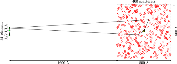
Figure 1: Geometry of the simulated dense scattering environment, with 400 uniformly distributed scatterers in a $800\times 800$ $\lambda$ area. The transmit $M$-element ULA is placed at a distance of 1600 $\lambda$ from the edge of the scatterer area with its broadside pointing towards the center. Two single scattering paths from the first ULA element to an intended receiver in the center of the scatterer area are shown.

In Figure 2 we show the resulting normalized field strength in a small $10\lambda\times 10\lambda$ environment around the receiver to which we focus the transmitted signal (using MF precoding), for ULAs with $d=\lambda/2$ of size $M=10$ and $M=100$ elements. The normalized field strength shows how much weaker the field strength is in a certain position when the spatial signature to the center point is used rather than the correct spatial signature for that point. Hence, the normalized field strength is 0 dB at the center of both figures, and negative at all other points. Figure 2 illustrates two important properties of the spatial MF precoding: (i) that the field strength can be focused to a point rather than in a certain direction and (ii) that more antennas improve the ability to focus energy to a certain point, which leads to less interference between spatially separated users. With $M=10$ antenna elements, the focusing of the field strength is quite poor with many peaks inside the studied area. Increasing $M$ to 100 antenna elements, for the same propagation environment, considerably improves the field strength focusing and it is more than 5 dB down in most of the studied area.

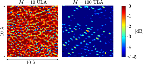
Figure 2: Normalized fieldstrength in a $10\times 10$ $\lambda$ area centered around the receiver to which the beamforming is done. The left and right pseudo color plots show the field strength when an $M=10$ and an $M=100$ ULA are used together with MF precoding to focus the signal to a receiver in the center of the area.

While the example above only illustrates spatial MF precoding in the narrowband case, the TRBF techniques exploit both the spatial and temporal domains to achieve an even stronger spatial focusing of the field strength. With enough many antennas and favorable propagation conditions, TRBF will not only focus power and yield a high spectral efficiency through spatial multiplexing to many terminals. It will also reduce, or in the ideal case completely eliminate, inter-symbol interference. In other words, one could dispense with OFDM and its redundant cyclic prefix. Each base station antenna would 1) merely convolve the data sequence intended for the $k$-th terminal with the conjugated, time-reversed version of his estimate for the channel impulse response to the $k$-th terminal, 2) sum the $K$ convolutions, and 3) feed that sum into his antenna. Again, under favorable propagation conditions, and a large number of antennas, inter-symbol interference will decrease significantly.

III-B Antenna aspects

It is common within the signal processing, communications and information theory communities to assume that the transmit and receive antennas are isotropic and uni-polarized electromagnetic wave radiators and sensors, respectively. In reality, such isotropic unipolar antennas do not exist, according to fundamental laws of electromagnetics. Non-isotropic antenna patterns will influence the MIMO performance by changing the spatial correlation. For example, directive antennas pointing in distinct directions tend to experience a lower correlation than non-directive antennas, since each of these directive antennas “see” signals arriving from a distinct angular sector.

In the context of an array of antennas, it is also common in these communities to assume that there is no electromagnetic interaction (or mutual coupling) among the antenna elements neither in the transmit nor in the receive mode. This assumption is only valid when the antennas are well separated from one another.

In the rest of this section we consider very large MIMO arrays where the overall aperture of the array is constrained, for example, by the size of the supporting structure or by aesthetic considerations. Increasing the number of antenna elements implies that the antenna separation decreases. This problem has been examined in recent papers, although the focus is often on spatial correlation and the effect of coupling is often neglected, as in [14, 15, 16]. In [17], the effect of coupling on the capacity of fixed length ULAs is studied. In general, it is found that mutual coupling has a substantial impact on capacity as the number of antennas is increased for a fixed array aperture.

It is conceivable that the capacity performance in [17] can be improved by compensating for the effect of mutual coupling. Indeed, coupling compensation is a topic of current interest, much driven by the desire of implementing MIMO arrays in a compact volume, such as mobile terminals (see [18] and references therein). One interesting result is that coupling among co-polarized antennas can be perfectly mitigated by the use of optimal multiport impedance matching radio frequency circuits [19]. This technique has been experimentally demonstrated only for up to four antennas, though in principle it can be applied to very large MIMO arrays [20]. Nevertheless, the effective cancellation of coupling also brings about diminishing bandwidth in one or more output ports as the antenna spacing decreases [21]. This can be understood intuitively in that, in the limit of small antenna spacing, the array effectively reduces to only one antenna. Thus, one can only expect the array to offer the same characteristics as a single antenna. Furthermore, implementing practical matching circuits will introduce ohmic losses, which reduces the gain that is achievable from coupling cancellation [18].

Another issue to consider is that due to the constraint in array aperture, very large MIMO arrays are expected to be implemented in a 2D or 3D array structure, instead of as a linear array as in [17]. A linear array with antenna elements of identical gain patterns (e.g., isotropic elements) suffers from the problem of front-back ambiguity, and is also unable to resolve signal paths in both azimuth and elevation. However, one drawback of having a dense array implementation in 2D or 3D is the increase of coupling effects due to the increase in the number of adjacent antennas. For the square array (2D) case, there are up to four adjacent antennas (located at the same distance) for each antenna element, and in 3D there are up to 6. A further problem that is specific to 3D arrays is that only the antennas located on the surface of the 3D array contribute to the information capacity [22], which in effect restricts the usefulness of dense 3D array implementations. This is a consequence of the integral representation of Maxwell’s equations, by which the electromagnetic field inside the volume of the 3D array is fully described by the field on its surface (assuming sufficiently dense sampling), and therefore no additional information can be extracted from elements inside the 3D array.

Moreover, in outdoor cellular environments, signals tend to arrive within a narrow range of elevation angles. Therefore, it may not be feasible for the antenna system to take advantage of the resolution in elevation offered by dense 2D or 3D arrays to perform signaling in the vertical dimension.

The complete Single-User MIMO (SU-MIMO) signal model with antennas and matching circuit in Figure 3 (reproduced from [23]) is used to demonstrate the performance degradation resulting from correlation and mutual coupling in very large arrays with fixed apertures. In the figure, ${\boldsymbol{Z}}_{\mathrm{t}}$ and ${\boldsymbol{Z}}_{\mathrm{r}}$ are the impedance matrices of the transmit and receive arrays, respectively, $i_{\mathrm{t}i}$ and $i_{\mathrm{r}i}$ are the excitation and received currents (at the $i$-th port) of the transmit and receive systems, respectively, and $v_{\mathrm{s}i}$ and $v_{\mathrm{r}i}$ (${\boldsymbol{Z}}_{\mathrm{s}}$ and ${\boldsymbol{Z}}_{\mathrm{l}}$) are the source and load voltages (impedances), respectively, and $v_{\mathrm{t}i}$ is the terminal voltage across the $i$-th transmit antenna port. $\boldsymbol{G}_{\mathrm{mc}}$ is the overall channel of the system, including the effects of antenna coupling and matching circuits.

Recall that the instantaneous capacity is given by (3) and equals

$$C_{\mathrm{mc}}=\log_{2}\det\left(\boldsymbol{I}_{n}+\frac{\rho}{n_{\mathrm{t}}}{\hat{\boldsymbol{G}}}_{\mathrm{mc}}{\hat{\boldsymbol{G}}}_{\mathrm{mc}}^{\rm H}\right),$$ (28)

where

$${\hat{\boldsymbol{G}}}_{\mathrm{mc}}=2r_{11}\boldsymbol{R}_{\mathrm{l}}^{1/2}({\boldsymbol{Z}}_{\mathrm{l}}+{\boldsymbol{Z}}_{\mathrm{r}})^{-1}{\boldsymbol{G}}{\boldsymbol{R}}_{\mathrm{t}}^{-1/2},$$ (29)

is the overall MIMO channel based on the complete SU-MIMO signal model, $\boldsymbol{G}$ represents the propagation channel as seen by the transmit and receive antennas, and ${\boldsymbol{R}}_{\mathrm{l}}=\mathop{\rm Re}\left\{{\boldsymbol{Z}}_{\mathrm{l}}\right\}$, ${\boldsymbol{R}}_{\mathrm{t}}=\mathop{\rm Re}\left\{{\boldsymbol{Z}}_{\mathrm{t}}\right\}$. Note that ${\hat{\boldsymbol{G}}}_{\mathrm{mc}}$ is the normalized version of $\boldsymbol{G}_{\mathrm{mc}}$ shown in Figure 3, where the normalization is performed with respect to the average channel gain of a SISO system [23]. The source impedance matrix $\boldsymbol{Z}_{\mathrm{s}}$ does not appear in the expression, since ${\hat{\boldsymbol{G}}}_{\mathrm{mc}}$ represents the transfer function between the transmit and receive power waves, and $\boldsymbol{Z}_{\mathrm{s}}$ is implicit in $\rho$ [23].

To give an intuitive feel for the effects of mutual coupling, we next provide two examples of the impedance matrix ${\boldsymbol{Z}}_{\mathrm{r}}$, one for small adjacent antenna spacing (0.05$\lambda$) and one for moderate spacing (0.5$\lambda$). The following numerical values are obtained from the induced electromotive force method [24] for a ULA consisting of three parallel dipole antennas:

$$\boldsymbol{Z}_{\mathrm{r}}(0.05\lambda)=\left[\begin{array}[]{ccc}72.9+j42.4&71.4+j24.3&67.1+j7.6\\ 71.4+j24.3&72.9+j42.4&71.4+j24.3\\ 67.1+j7.6&71.4+j24.3&72.9+j42.4\end{array}\right],$$

and

$$\boldsymbol{Z}_{\mathrm{r}}(0.5\lambda)=\left[\begin{array}[]{ccc}72.9+j42.4&-12.5-j29.8&4.0+j17.7\\ -12.5-j29.8&72.9+j42.4&-12.5-j29.8\\ 4.0+j17.7&-12.5-j29.8&72.9+j42.4\end{array}\right].$$

It can be observed that the severe mutual coupling in the case of $d=0.05\lambda$ results in off-diagonal elements whose values are closer to the diagonal elements than in the case of $d=0.5\lambda$, where the diagonal elements are more dominant. Despite this, the impact of coupling on capacity is not immediately obvious, since the impedance matrix is embedded in (29), and is conditioned by the load matrix ${\boldsymbol{Z}}_{\mathrm{l}}$. Therefore, we next provide numerical simulations to give more insight into the impact of mutual coupling on MIMO performance.

In MU-MIMO systems, the terminals are autonomous so that we can assume that the transmit array is uncoupled and uncorrelated. If the Kronecker model [25] is assumed for the propagation channel ${\boldsymbol{G}}=\boldsymbol{\Psi}_{\mathrm{r}}^{1/2}\boldsymbol{G}_{\mathrm{IID}}\boldsymbol{\Psi}_{\mathrm{t}}^{1/2}$, where $\boldsymbol{\Psi}_{\mathrm{t}}$ and $\boldsymbol{\Psi}_{\mathrm{r}}$ are the transmit and receive correlation matrices, respectively, and $\boldsymbol{G}_{\mathrm{IID}}$ is the matrix with IID Rayleigh entries [23]. In this case, ${\boldsymbol{\Psi}}_{\mathrm{t}}^{1/2}=\boldsymbol{I}_{K}$ and $\boldsymbol{Z}_{\mathrm{t}}$ is diagonal. For the particular case of $M=K$, Figure 4 shows a plot of the uplink ergodic capacity (or average rate) per user, $C_{\mathrm{mc}}/K$, versus the antenna separation for ULAs with a fixed aperture of $5\lambda$ at the base station (with up to $M=K=30$ elements). The correlation but no coupling case refers to the MIMO channel ${\boldsymbol{G}}=\boldsymbol{\Psi}_{\mathrm{r}}^{1/2}\boldsymbol{G}_{\mathrm{IID}}\boldsymbol{\Psi}_{\mathrm{t}}^{1/2}$, whereas the correlation and coupling case refers to the effective channel matrix ${\hat{\boldsymbol{G}}}_{\mathrm{mc}}$ in (29). The environment is assumed to be uniform 2D Angular Power Spectrum (APS) and the SNR is $\rho=20$ dB. The total power is fixed and equally divided among all users. 1000 independent realizations of the channel are used to obtain the average capacity. For comparison, the corresponding ergodic capacity per user is also calculated for $K^{2}$ users and an $M^{2}$-element receive Uniform Square Array (USA) with $M=K$ and an aperture size of $5\lambda\times 5\lambda$, for up to $M^{2}=900$ elements.

As can be seen in Figure 4, the capacity per user begins to fall when the element spacing is reduced to below $2.5\lambda$ for the USAs, as opposed to below $0.5\lambda$ for the ULAs, which shows that for a given antenna spacing, packing more elements in more than one dimension results in significant degradation in capacity performance. Another distinction between the ULAs and USAs is that coupling is in fact beneficial for the capacity performance of ULAs with moderate antenna spacing (i.e. between $0.15\lambda$ and $0.7\lambda$), whereas for USAs the capacity with coupling is consistently lower than that with only correlation. The observed phenomenon for ULAs is similar to the behavior of two dipoles with decreasing element spacing [18]. There, coupling induces a larger difference between the antenna patterns (i.e., angle diversity) over this range of antenna spacing, which helps to reduce correlation. At even smaller antenna spacings, the angle diversity diminishes and correlation increases. Together with loss of power due to coupling and impedance mismatch, the increasing correlation results in the capacity of the correlation and coupling case falling below that of the correlation only case, with the crossover occuring at approximately $0.15\lambda$. On the other hand, each element in the USAs experiences more severe coupling than that in the ULAs for the same adjacent antenna spacing, which inherently limits angle diversity.

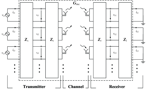
Figure 3: Diagram of a MIMO system with antenna impedance matrices and matching networks at both link ends (freely reproduced from [23]).

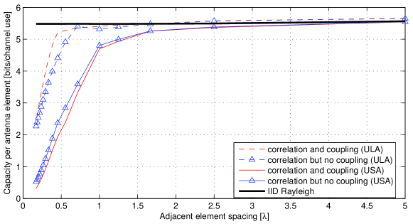
Figure 4: Impact of correlation and coupling on capacity per antenna over different adjacent antenna spacing for autonomous transmitters. $M=K$ and the apertures of ULA and USA are $5\lambda$ and $5\lambda\times 5\lambda$, respectively.

Even though Figure 4 demonstrates that both coupling and correlation are detrimental to the capacity performance of very large MIMO arrays relative to the IID case, it does not provide any specific information on the behavior of ${\hat{\boldsymbol{G}}}_{\mathrm{mc}}$. In particular, it is important to examine the impact of correlation and coupling on the asymptotic orthogonality assumption made in (16) for a very large array with a fixed aperture in a MU setting. To this end, we assume that the base station serves $K=15$ single antenna terminals. The channel is normalized so that each user terminal has a reference SNR $\rho/K=10$ dB in the SISO case with conjugate-matched single antennas. As before, the coupling and correlation at the base station is the result of implementing the antenna elements as a square array of fixed dimensions $5\lambda\times 5\lambda$ in a channel with uniform 2D APS. The number of elements in the receive USA $M$ varies from 16 to 900, in order to support one dedicated channel per user.

The average condition number of ${\hat{\boldsymbol{G}}_{\mathrm{mc}}^{\rm H}\hat{\boldsymbol{G}}_{\mathrm{mc}}}/K$ is given in Figure 5(a) for 1000 channel realizations. Since the propagation channel is assumed to be IID in (29) for simplicity, $\boldsymbol{D}_{\mathbf{\beta}}=\boldsymbol{I}_{K}$. This implies that the condition number of ${\hat{\boldsymbol{G}}_{\mathrm{mc}}^{\rm H}\hat{\boldsymbol{G}}_{\mathrm{mc}}}/K$ should ideally approach one, which is observed for the IID Rayleigh case. By way of contrast, it can be seen that the channel is not asymptotically orthogonal as assumed in (16) in the presence of coupling and correlation. The corresponding maximum rate for the reverse link per user is given in Figure 5(b). It can be seen that if coupling is ignored, spatial correlation yields only a minor penalty, relative to the IID case. This is so because the transmit array of dimensions $5\lambda\times 5\lambda$ is large enough to offer almost the same number of spatial degrees of freedom ($K=15$) as in the IID case, despite the channel not being asymptotically orthogonal. On the other hand, for the realistic case with coupling and correlation, adding more receive elements into the USA will eventually result in a reduction of the achievable rate, despite having a lower average condition number than in the correlation but no coupling case. This is attributed to the significant power loss through coupling and impedance mismatch, which is not modeled in the correlation only case.

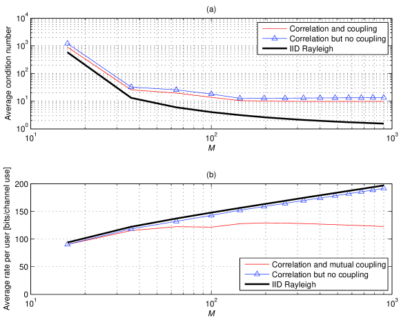
Figure 5: Impact of correlation and coupling on (a) asymptotic orthogonality of the channel matrix and (b) max sum-rate of the reverse link, for $K=15$.

III-C Real propagation - measured channels

When it comes to propagation aspects of MIMO as well as very large MIMO the correlation properties are of paramount interest, since those together with the number of antennas at the terminals and base station determines the orthogonality of the propagation channel matrix and the possibility to separate different users or data streams. In conventional MU-MIMO systems the ratio of number of base station antennas and antennas at the terminals is usually close to 1, at least it rarely exceeds 2. In very large MU-MIMO systems this ratio may very well exceed 100; if we also consider the number of expected simultaneous users, $K$, the ratio at least usually exceeds 10. This is important because it means that we have the potential to achieve a very large spatial diversity gain. It also means that the distance between the null-spaces of the different users is usually large and, as mentioned before, that the singular values of the tall propagation matrix tend to have stable and large values. This is also true in the case where we consider multiple users where we can consider each user as a part of a larger distributed, but un-coordinated, MIMO system. In such a system each new user “consumes” a part of the available diversity. Under certain reasonable assumptions and favorable propagation conditions, it will, however, still be possible to create a full rank propagation channel matrix (16) where all the eigenvalues have large magnitudes and show a stable behavior. The question is now what we mean by the statement that the propagation conditions should be favorable? One thing is for sure: As compared to a conventional MIMO system, the requirements on the channel matrix to get good performance in very large MIMO are relaxed to a large extent due to the tall structure of the matrix.

It is well known in conventional MIMO modeling that scatterers tend to appear in groups with similar delays, angle-of-arrivals and angle-of-departures and they form so-called clusters. Usually the number of active clusters and distinct scatterers are reported to be limited, see e.g. [26], also when the number of physical objects is large. The contributions from individual multipath components belonging to the same cluster are often correlated which reduces the number of effective scatterers. Similarly it has been shown that a cluster seen by different users, so called joint clusters, introduces correlation between users also when they are widely separated [27]. It is still an open question whether the use of large arrays makes it possible to resolve clusters completely, but the large spatial resolution will make it possible to split up clusters in many cases. There are measurements showing that a cluster can be seen differently from different parts of a large array [28], which is beneficial since the correlation between individual contributions from a cluster then is decreased.

To exemplify the channel properties in a real situation we consider a measured channel matrix where we have an indoor 128-antenna base station consisting of four stacked double polarized 16 element circular patch arrays, and 6 single antenna users. Three of the users are indoors at various positions in an adjacent room and 3 users are outdoors but close to the base station. The measurements were performed at 2.6 GHz with a bandwidth of 50 MHz. In total we consider an ensemble of 100 snapshots (taken from a continuous movement of the user antenna along a 5-10 m line) and 161 frequency points, giving us in total 16100 narrow-band realizations. It should be noted, though, that they are not fully independent due to the non-zero coherence bandwidth and coherence distance. The channels are normalized to remove large scale fading and to maintain the small scale fading. The mean power over all frequency points and base station antenna elements is unity for all users. In Figure 6 we plot the Cumulative Distribution Functions (CDF) of the ordered eigenvalues of $\boldsymbol{G}^{\rm H}\boldsymbol{G}$ (the leftmost solid curve corresponds to the CDF of the smallest eigenvalue etc.) for the $6\times 128$ propagation matrix (“Meas 6x128”), together with the corresponding CDFs for a $6\times 6$ measured conventional MIMO (“Meas 6x6”) system (where we have used a subset of 6 adjacent co-polarized antennas on the base station). As a reference we also plot the distribution of the largest and smallest eigenvalues for a simulated $6\times 128$ and $6\times 6$ conventional MIMO system (“IID 6x128” and “IID 6x6”) with independent identically distributed complex Gaussian entries. Note that, for clarity of the figure, the eigenvalues are not normalized with the number of antennas at the base station and therefore there is an offset of $10\log_{10}(M)$. This offset can be interpreted as a beamforming gain. In any case, the relative spread of the eigenvalues is of more interest than their absolute levels.

\psfrag{IID 6x128}{\scalebox{0.7}{ IID $6\!\!\times\!\!128$ }}\psfrag{IID 6x6}{\scalebox{0.7}{ IID $6\!\!\times\!\!6$ }}\psfrag{meas 6x128}{\scalebox{0.7}{ Meas $6\!\!\times\!\!128$}}\psfrag{meas 6x6}{\scalebox{0.7}{ Meas $6\!\!\times\!\!6$}}\psfrag{ordered singular values [dB]}{\scalebox{0.75}{ Ordered eigenvalues of $\boldsymbol{G}^{\rm H}\boldsymbol{G}$ [dB]}}\includegraphics[width=303.53267pt]{SingValCDF.eps}

Figure 6: CDFs of ordered eigenvalues for a measured $6\times 128$ large array system, a measured $6\times 6$ MIMO system and simulated IID $6\times 6$ and $6\times 128$ MIMO systems. Note that for the simulated IID cases, only the CDFs of the largest and smallest eigenvalues are shown for clarity.

It can be clearly seen that the large array provides eigenvalues that all show a stable behavior (low variances) and have a relatively low spread (small distances between the CDF curves). The difference between the smallest and largest eigenvalue is only around 7 dB, which could be compared with the conventional $6\times 6$ MIMO system where this difference is around 26 dB. This eigenvalue spread corresponds to that of a 6x24 conventional MIMO system with IID complex Gaussian channel matrix entries. Keeping in mind the circular structure of the base station antenna array and that half of the elements are cross polarized, this number of ’effective’ channels is about what one could anticipate to get. One important factor in realistic channels, especially for the uplink, is that the received power levels from different users are not equal. Power variations will increase both the eigenvalue spread and the variance, and will result in a matrix that still is approximately orthogonal, but where the diagonal elements of $\boldsymbol{G}^{\rm H}\boldsymbol{G}$ have varying mean levels, namely the $\boldsymbol{D}_{\beta}$ matrix in (16).

IV Transceivers

We next turn our attention to the design of practical transceivers. A method to acquire CSI at the base station begins the discussion. Then we discuss precoders and detection algorithms suitable for very large MIMO arrays.

IV-A Acquiring CSI at the base station

In order to do multiuser precoding in the forward link and detection in the reverse link, the base station must acquire CSI. Let us assume that the frequency response of the channel is constant over $N_{\mathrm{Coh}}$ consecutive subcarriers. With small antenna arrays, one possible system design is to let the base station antennas transmit pilot symbols to the receiving units. The receiving units perform channel estimation and feed back, partial or complete, CSI via dedicated feedback channels. Such a strategy does not rely on channel reciprocity (i.e., the forward channel should be the transpose of the reverse channel). However, with a limited coherence time, this strategy is not viable for large arrays. The number of time slots devoted to pilot symbols must be at least as large as the number of antenna elements at the base station divided by $N_{\mathrm{Coh}}$. When $M$ grows, the time spent on transmitting pilots may surpass the coherence time of the channel.

Consequently, large antenna array technology must rely on channel reciprocity. With channel reciprocity, the receiving units send pilot symbols via TDD. Since the frequency response is assumed constant over $N_{\mathrm{Coh}}$ subcarriers, $N_{\mathrm{Coh}}$ terminals can transmit pilot symbols simultaneously during 1 OFDM symbol interval. In total, this requires $K/N_{\mathrm{Coh}}$ time slots (we remind the reader that $K$ is the number of terminals served). The base station in the $k$-th cell constructs its channel estimate ${\hat{\boldsymbol{G}}}^{\rm T}_{kk}$, subsequently used for precoding in the forward link, based on the pilot observations. The power of each pilot symbol is denoted $\rho_{\mathrm{p}}$.

IV-B Precoding in the forward link: Collection of results for single cell systems

User $k$ receives the $k$-th component of the composite vector

$$\boldsymbol{x}_{\mathrm{f}}=\boldsymbol{G}^{\rm T}\boldsymbol{s}_{\mathrm{f}}+\boldsymbol{w}_{\mathrm{f}}.$$

The vector $\boldsymbol{s}_{\mathrm{f}}$ is a precoded version of the data symbols $\boldsymbol{q}_{\mathrm{f}}$. Each component of $\boldsymbol{s}_{\mathrm{f}}$ has average power $\rho_{\mathrm{f}}/M$. Further, we assume that the channel matrix $\boldsymbol{G}$ has IID $\mathcal{CN}(0,1)$ entries. In what follows, we derive SNR/SINR (Signal-to-Interference-plus-Noise-Ratio) expressions for a number of popular precoding techniques in the large system limit, i.e., with $M,K\to\infty$, but with a fixed ratio $\alpha=M/K$. The obtained expressions are tabulated in Table I.

Let us first discuss the performance of an Interference Free (IF) system which will subsequently serve as a benchmark reference. The best performance that can be imagined will result if all the channel energy to terminal $k$ is delivered to terminal $k$ without any inter-user interference. In that case, terminal $k$ receives the sample $x_{\mathrm{f}k}$

$$x_{\mathrm{f}k}=\sqrt{\sum_{\ell=1}^{M}|g_{\ell k}|^{2}}\,q_{\mathrm{f}k}+w_{\mathrm{f}k}.$$

Since $\left(\sum_{\ell=1}^{M}|g_{\ell k}|^{2}\right)/M\to 1,\;M\to\infty,$ and $\mathbb{E}\left\{q_{\mathrm{f}k}q_{\mathrm{f}k}^{\rm H}\right\}=\rho_{\mathrm{f}}/K,$ the SNR per receiving unit for IF systems converges to $\rho_{\mathrm{f}}\alpha$ as $M\to\infty$.

We now move on to practical precoding methods. The conceptually simplest approach is to invert the channel by means of the pseudo-inverse. This is referred to as Zero-Forcing (ZF) precoding [29]. A variant of zero forcing is Block Diagonalization [30], which is not covered in this paper. Intuitively, when $M$ grows, $\boldsymbol{G}$ tends to have nearly orthogonal columns as the terminals are not correlated due to their physical separation. This assures that the performance of ZF precoding will be close to that of the IF system. However, a disadvantage of ZF is that processing cannot be done distributedly at each antenna separately. With ZF precoding, all data must instead be collected at a central node that handles the processing.

Formally, the ZF precoder sets

$$\boldsymbol{s}_{\mathrm{f}}=\frac{1}{\sqrt{\gamma}}(\boldsymbol{G}^{\rm T})^{+}\boldsymbol{q}_{\mathrm{f}}=\frac{1}{\sqrt{\gamma}}\boldsymbol{G}^{\ast}(\boldsymbol{G}^{\rm T}\boldsymbol{G}^{\ast})^{-1}\boldsymbol{q}_{\mathrm{f}},$$

where the superscript “+” denotes the pseudo-inverse of a matrix, i.e. $(\boldsymbol{G}^{\rm T})^{+}=\boldsymbol{G}^{\ast}(\boldsymbol{G}^{\rm T}\boldsymbol{G}^{\ast})^{-1}$, and $\gamma$ normalizes the average power in $\boldsymbol{s}_{\mathrm{f}}$ to $\rho_{\mathrm{f}}$. A suitable choice for $\gamma$ is $\gamma=\mathrm{Tr}(\boldsymbol{G}^{\rm T}\boldsymbol{G}^{\ast})^{-1}/K$ which averages fluctuations in transmit power due to $\boldsymbol{G}$ but not to $\boldsymbol{q}_{\mathrm{f}}$. The received sample $x_{\mathrm{f}k}$ with ZF precoding becomes

$$x_{\mathrm{f}k}={\frac{q_{\mathrm{f}k}}{\sqrt{\gamma}}}+w_{\mathrm{f}k}.$$

With that, the instantaneous received SNR per terminal equals

$$\mathrm{SNR} = \frac{\rho_{\mathrm{f}}}{K\,\gamma}$$ (30)

$$= \frac{\rho_{\mathrm{f}}}{\mathrm{Tr}(\boldsymbol{G}^{\rm T}\boldsymbol{G}^{\ast})^{-1}}.$$

When both the number of terminals $K$ and the number of base station antennas $M$ grow large, but with fixed ratio $\alpha=M/K$, $\mathrm{Tr}(\boldsymbol{G}^{\rm T}\boldsymbol{G}^{\ast})^{-1}$ converges to a fixed deterministic value [31]

$$\mathrm{Tr}(\boldsymbol{G}^{\rm T}\boldsymbol{G}^{\ast})^{-1}\to\frac{1}{\alpha-1},\quad\mathrm{as}\;K,\,M\to\infty,\quad\frac{M}{K}=\alpha.$$ (31)

Substituting (31) into (30) gives the expression in Table I. The conclusion is that ZF precoding achieves an $\mathrm{SNR}$ that tends to the optimal $\mathrm{SNR}$ for an IF system with $M-K$ transmit antennas when the array size grows. Note that when $M=K$, one gets $\mathrm{SNR}=0$.

A problem with ZF precoding is that the construction of the pseudo-inverse $(\boldsymbol{G}^{\rm T})^{+}=\boldsymbol{G}^{\ast}(\boldsymbol{G}^{\rm T}\boldsymbol{G}^{\ast})^{-1}$ requires the inversion of a $K\times K$ matrix, which is computationally expensive. However, as $M$ grows, $(\boldsymbol{G}^{\rm T}\boldsymbol{G}^{\ast})/M$ tends to the identity matrix, which has a trivial inverse. Consequently, the ZF precoder tends to $\boldsymbol{G}^{\ast}$, which is nothing but a MF. This suggests that matrix inversion may not be needed when the array is scaled up, as the MF precoder approximates the ZF precoder well. Formally, the MF sets

$$\boldsymbol{s}_{\mathrm{f}}=\frac{1}{\sqrt{\gamma}}\boldsymbol{G}^{\ast}\boldsymbol{q}_{\mathrm{f}},$$

with $\gamma=\mathrm{Tr}(\boldsymbol{G}^{\rm T}\boldsymbol{G}^{\ast})/K$. A few simple manipulations lead to an asymptotic expression of the SINR, which is given in Table I.

From the MF precoding SINR expression, it is seen that the SINR can be made as high as desired by scaling up the antenna array. However, the MF precoder exhibits an error floor since as $\rho_{\mathrm{f}}\to\infty,\;\mathrm{SINR}\to\alpha$.

We next turn the attention to scenarios where the base station has imperfect CSI. Let $\hat{\boldsymbol{G}}^{\rm T}$ denote the Minimum Mean Square Error (MMSE) channel estimate of the forward link. The estimate satisfies,

$$\hat{\boldsymbol{G}}^{\rm T}=\xi\boldsymbol{G}^{\rm T}+\sqrt{1-\xi^{2}}\boldsymbol{E},$$

where $0\leq\xi\leq 1$ represents the reliability of the estimate and $\boldsymbol{E}$ is a matrix with IID $\mathcal{CN}(0,1)$ distributed entries. SINR expressions for MF and ZF precoding are given in Table I. For any reliability $\xi$, the $\mathrm{SINR}$ can be made as high as desired by scaling up the antenna array.

SNR and SINR expressions as $K,M\to\infty,\quad M/K=\alpha$
Precoding Technique	Perfect CSI	Imperfect CSI
Benchmark: IF System	$\rho_{\mathrm{f}}\alpha$
Zero Forcing	$\rho_{\mathrm{f}}(\alpha-1)$	$\frac{\xi^{2}\,\rho_{\mathrm{f}}(\alpha-1)}{(1-\xi^{2})\,\rho_{\mathrm{f}}+1}$
Matched Filter	$\frac{\rho_{\mathrm{f}}\alpha}{\rho_{\mathrm{f}}+1}$	$\frac{\xi^{2}\rho_{\mathrm{f}}\alpha}{\rho_{\mathrm{f}}+1}$
Vector Perturbation	$\approx\frac{\rho_{\mathrm{f}}\,\alpha\,\pi}{6}\left(1-\frac{1}{\alpha}\right)^{1-\alpha},\quad\alpha\lessapprox 1.79$	N.A.

TABLE I: SNR and SINR expressions for a collection of standard precoding techniques.

Non-linear precoding techniques, such as DPC, Vector Perturbation (VP) [32], and lattice-aided methods [33] are important techniques when $M$ is not much larger than $K$. This is true since in the $M\approx K$ regime, the performance gap of ZF to the IF benchmark is significant, see Table I, and there is room for improvement by non-linear techniques. However, the gap of ZF to an IF system scales as $\alpha/(\alpha-1)$. When $M$ is, say, two times $K$, this gap is only 3 dB. Non-linear techniques will operate closer to the IF benchmark, but cannot surpass it. Therefore the gain of non-linear methods does not at all justify the complexity increase. The measured $6\times 128$ channels that we discussed earlier in the paper behave as if $\alpha\approx 4$. Hence, linear precoding is virtually optimal and one can dispense with DPC.

For completeness we give an approximate large limit SNR expression for VP, derived from the results of [34], in Table I. The expression is strictly speaking an upper bound to the SNR, but is reasonably tight [34] so that it can be taken as an approximation. For $\alpha\gtrapprox 1.79$, the SINR expression surpasses that of an IF system, which makes the expression meaningless. However, for larger values of $\alpha$, linear precoding performs well and there is not much gain in using VP anyway. For VP, no SINR expression is available in the literature with imperfect CSI.

In Figure 7 we show ergodic sum-rate capacities for MF precoding, ZF precoding, and DPC. As benchmark performance we also show the ensuing sum-rate capacity from an IF system. In all cases, $K=15$ users are served and we show results for $M=15,\,40,\,100$. For $M=15$, it can be seen that DPC decisively outperforms ZF and is about 3 dB away from the IF benchmark performance. But as $M$ grows, the advantage of DPC quickly diminishes. With $M=40$, the gain of DPC is about 1 dB. This confirms that the performance gain does not at all justify the complexity increase. With 100 base station antennas, ZF precoding performs almost as good as an interference free system. At low SNR, MF precoding is better than ZF precoding. It is interesting to observe that this is true over a wide range of SNRs for the case of $M=K$. Sum-rate capacity expressions of VP are currently not available in the literature, since the optimal distribution of the inputs for VP is not known to date.

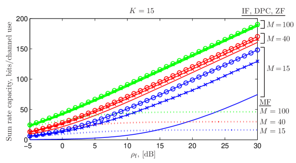
Figure 7: Sum-rate capacities of single cell multiuser MIMO precoding techniques. The channel is IID complex Gaussian $\mathcal{CN}(0,1)$, there are $K=15$ terminals. Circles show the performance of IF systems, x-es refer to DPC, solid lines refer to ZF, and the dotted lines refer to MF.

IV-C Precoding in the forward link: The ultimate limit of non-cooperative multi cell MIMO with large arrays

In this section, we investigate the limit of non-cooperative cellular multiuser MIMO systems as $M$ grows without limit. The presentation summarizes and extends the results of [5]. For single cell as well as for multi cell MIMO, the end effect of letting $M$ grow without limits is that thermal noise and small scale Rayleigh fading vanishes. However, as we will discuss in detail, with multiple cells the interference from other cells due to pilot contamination does not vanish. The concept of pilot contamination is novel in a cellular MU-MIMO context and is illustrated in Figure 8, but was an issue in the context of CDMA, usually under the name “pilot pollution”. The channel estimate computed by the base station in cell 1 gets contamined from the pilot transmission of cell 2. The base station in cell 1 will in effect beamform its signal partially along the channel to the terminals in cell 2. Due to the beamforming, the interference to cell 2 does not vanish asymptotically as $M\to\infty$.

\psfrag{Gm}{\scalebox{1.0}{ SIR [dB]}}\includegraphics{PilotCont.eps}

Figure 8: Illustration of the pilot contamination concept. Left: During the training phase, the base station in cell 1 overhears the pilot transmission from other cells. Right: As a consequence, the transmitted vector from base station 1 will be partially beamformed to the terminals in cell 2.

We consider a cellular multiuser MIMO-OFDM system with hexagonal cells and $N_{\mathrm{FFT}}$ subcarriers. All cells serves $K$ autonomous terminals and has $M$ antennas at the base station. Further, a sparse scenario $K\leq M$ is assumed for simplicity. Hence, terminal scheduling aspects are not considered. The base stations are assumed non-cooperative. The $M\times K$ composite channel matrix between the $K$ terminals in cell $k$ and the base station in cell $j$ is denoted $\boldsymbol{G}_{kj}$. Relying on reciprocity, the forward link channel matrix between the base station in cell $j$ and the terminals in cell $k$ becomes $\boldsymbol{G}_{kj}^{\rm T}$ (see Figure 9).

\psfrag{Gm}{\scalebox{1.0}{ SIR [dB]}}\includegraphics{Cells.eps}

Figure 9: The composite channel between the base station in cell $j$ and the terminals in cell $k$ is denoted $\boldsymbol{G}_{kj}^{\rm T}$.

The base station in the $k$-th cell transmits the vector $\boldsymbol{s}_{\mathrm{f}k}$ which is a precoded version of the data symbols $\boldsymbol{q}_{\mathrm{f}k}$ intended for the terminals in cell $k$. Each terminal in the $k$-th cell receives his respective component of the composite vector

$$\boldsymbol{x}_{\mathrm{f}k}=\rho_{\mathrm{f}}\sum_{j}\boldsymbol{G}^{\rm T}_{kj}\boldsymbol{s}_{\mathrm{f}j}+\boldsymbol{w}_{\mathrm{f}k}.$$ (32)

As before, each element of $\boldsymbol{G}_{kj}$ comprises a small scale Rayleigh fading factor as well as a large scale factor that accounts for geometric attenuation and shadow fading. With that, $\boldsymbol{G}_{kj}$ factors as

$$\boldsymbol{G}_{kj}=\boldsymbol{H}_{kj}\boldsymbol{D}_{\beta_{kj}}^{1/2}.$$ (33)

In (33), $\boldsymbol{H}_{kj}$ is a $M\times K$ matrix which represents the small scale fading between the terminals in cell $k$ to the base station in cell $j$, all entries are IID $\mathcal{CN}(0,1)$ distributed. The $K\times K$ matrix $\boldsymbol{D}_{\beta_{kj}}^{1/2}$ is a diagonal matrix comprising the elements $\boldsymbol{\beta}_{kj}=[\beta_{kj1},\,\beta_{kj2},\ldots,\,\beta_{kjK}]$ along its main diagonal; each value $\beta_{kj\ell}$ represents the large scale fading between terminal $\ell$ in the $k$-th cell and the base station in cell $j$.

The base station in the $n$-th cell processes its pilot observations and obtains a channel estimate ${\hat{\boldsymbol{G}}}^{\rm T}_{nn}$ of $\boldsymbol{G}^{\rm T}_{nn}$. In the worst case, the pilot signals in all other cells are perfectly synchronized with the pilot signals in cell $n$. Hence, the channel estimate ${\hat{\boldsymbol{G}}}^{\rm T}_{nn}$ gets contamined from pilot signals in other cells,

$${{\hat{{\boldsymbol{G}}}}^{\rm T}}_{nn}=\sqrt{\rho_{\mathrm{p}}}\boldsymbol{G}_{nn}^{\rm T}+\sqrt{\rho_{\mathrm{p}}}\sum_{i\neq n}{\boldsymbol{G}}^{\rm T}_{in}+\boldsymbol{V}_{n}^{\rm T}.$$ (34)

In (34) it is implicitly assumed that all terminals transmits identical pilot signals. Adopting different pilot signals in different cells does not improve the situation much [5] since the pilot signals must at least be confined to the same signal space, which is of finite dimensionality.

Note that, due to the geometry of the cells, $\boldsymbol{G}_{nn}$ is generally stronger than $\boldsymbol{G}_{in},\,i\neq n$. $\boldsymbol{V}_{n}$ is a matrix of receiver noise during the training phase, uncorrelated with all propagation matrices, and comprises IID $\mathcal{CN}(0,1)$ distributed elements; $\rho_{\mathrm{p}}$ is a measure of the SNR during of the pilot transmission phase.

Motivated by the virtual optimality of simple linear precoding from Section IV-B, we let the base station in cell $n$ use the MF $(\hat{\boldsymbol{G}}^{\rm T}_{nn})^{\rm H}={\hat{{\boldsymbol{G}}}}_{nn}^{\ast}$ as precoder. We later investigate zero-forcing precoding. Power normalization of the precoding matrix is unimportant when $M\to\infty$ as will become clear shortly. The $\ell$-th terminal in the $j$-th cell receives the $\ell$-th component of the vector $\boldsymbol{x}_{\mathrm{f}j}=[x_{\mathrm{f}j1},\,x_{\mathrm{f}j1},\ldots,\,x_{\mathrm{f}jK}]^{\rm T}$. Inserting (34) into (32) gives

$$\boldsymbol{x}_{\mathrm{f}j} = \sqrt{\rho_{\mathrm{f}}}\sum_{n}\boldsymbol{G}^{\rm T}_{jn}{\hat{\boldsymbol{G}}}^{\ast}_{nn}\,\boldsymbol{q}_{\mathrm{f}n}+\boldsymbol{w}_{\mathrm{f}j}$$ (35)

$$= \sqrt{\rho_{\mathrm{f}}}\sum_{n}\boldsymbol{G}^{\rm T}_{jn}\left[\sqrt{\rho_{\mathrm{p}}}\sum_{i}{\boldsymbol{G}}^{\rm T}_{in}+\boldsymbol{V}_{n}^{\rm T}\right]^{\rm H}\,\boldsymbol{q}_{\mathrm{f}n}+\boldsymbol{w}_{\mathrm{f}j}.$$

The composite received signal vector $\boldsymbol{x}_{\mathrm{f}j}$ in (35) contains terms of the form $\boldsymbol{G}^{\rm T}_{jn}\boldsymbol{G}^{\ast}_{in}.$ As $M$ grows large, only terms where $j=i$ remain significant. We get

$$\frac{\boldsymbol{x}_{\mathrm{f}j}}{M\sqrt{{\rho_{\mathrm{f}}\rho_{\mathrm{p}}}}}\to\sum_{n}\frac{\boldsymbol{G}^{\rm T}_{jn}\boldsymbol{G}^{\ast}_{jn}}{M}\boldsymbol{q}_{\mathrm{f}n},\quad\mathrm{as}\;M\to\infty.$$

Further, as $M$ grows, the effect of small scale Rayleigh fading vanishes,

$$\frac{\boldsymbol{G}_{jn}^{\rm T}\boldsymbol{G}_{jn}^{\ast}}{M}\to{\boldsymbol{D}}_{\beta_{jn}}.$$

Hence, the processed received signal of the $\ell$-th receiving unit in the $j$-th cell is

$$\frac{x_{\mathrm{f}j\ell}}{M\sqrt{\rho_{\mathrm{f}}\rho_{\mathrm{p}}}}\to\beta_{jj\ell}q_{\mathrm{f}j\ell}+\sum_{n\neq j}\beta_{jn\ell}q_{\mathrm{f}n\ell}.$$ (36)

The SIR of terminal $\ell$ becomes

$$\mathrm{SIR}=\frac{{\beta^{2}_{jj\ell}}}{\sum_{n\neq j}{\beta^{2}_{jn\ell}}},$$ (37)

which does not contain any thermal noise or small scale fading effects! Note that devoting more power to the training phase does not decrease the pilot contamination effect and leads to the same SIR. This is a consequence of the worst-case-scenario assumption that the pilot transmissions in all cells overlap. If the pilot transmissions are staggered so that pilots in one cell collide with data in other cells, devoting more power to the training phase is indeed beneficial. However, in a multi cell system, there will always be some pilot transmissions that collide, although perhaps not in neighboring cells.

We now replace the MF precoder in (35) with the pseudo-inverse of the channel estimate $({\hat{{\boldsymbol{G}}}_{nn}}^{\rm T})^{+}=\hat{{\boldsymbol{G}}}_{nn}^{\ast}(\hat{{\boldsymbol{G}}}^{\rm T}_{nn}\hat{{\boldsymbol{G}}}_{nn}^{\ast})^{-1}.$ Inserting the expression for the channel estimate (34) gives

$$({\hat{{\boldsymbol{G}}}}^{\rm T}_{nn})^{+}=\left[\sqrt{\rho_{\mathrm{p}}}\sum_{i}{\boldsymbol{G}}^{\ast}_{in}+\boldsymbol{V}^{\ast}_{n}\right]\left(\left[\sqrt{\rho_{\mathrm{p}}}\sum_{i^{\prime}}{\boldsymbol{G}}^{\rm T}_{i^{\prime}n}+\boldsymbol{V}^{\rm T}_{n}\right]\left[\sqrt{\rho_{\mathrm{p}}}\sum_{i^{\prime\prime}}{\boldsymbol{G}}^{\ast}_{i^{\prime\prime}n}+\boldsymbol{V}^{\ast}_{n}\right]\right)^{-1}.$$

Again, when $M$ grows, only products of correlated terms remain significant,

$$({\hat{{\boldsymbol{G}}}}^{\rm T}_{nn})^{+}\to\frac{1}{M\rho_{\mathrm{p}}}\left[\sqrt{\rho_{\mathrm{p}}}\sum_{i}{\boldsymbol{G}}_{in}^{\ast}+\boldsymbol{V}^{\ast}_{n}\right]\left(\sum_{i}\boldsymbol{D}_{\beta_{in}}+\frac{1}{\rho_{\mathrm{p}}}\boldsymbol{I}_{K}\right)^{-1}.$$

The processed composite received vector in the $j$-th cell becomes

$$\sqrt{\frac{\rho_{\mathrm{p}}}{\rho_{\mathrm{f}}}}\boldsymbol{x}_{\mathrm{f}j}\to\sum_{n}{\boldsymbol{D}}_{\beta_{jn}}\left(\sum_{i}\boldsymbol{D}_{\beta_{in}}+\frac{1}{\rho_{\mathrm{p}}}\boldsymbol{I}_{K}\right)^{-1}\boldsymbol{q}_{\mathrm{f}n}.$$

Hence, the $\ell$-th receiving unit in the $j$-th cell receives

$$\sqrt{\frac{\rho_{\mathrm{p}}}{\rho_{\mathrm{f}}}}x_{\mathrm{f}j\ell}\to\frac{\beta_{jj\ell}}{\sum_{i}\beta_{ij\ell}+\frac{1}{\rho_{\mathrm{p}}}}q_{\mathrm{f}j\ell}+\sum_{n\neq j}\frac{\beta_{jn\ell}}{\sum_{i}\beta_{in\ell}+\frac{1}{\rho_{\mathrm{p}}}}q_{\mathrm{f}n\ell}.$$

The SIR of terminal $k$ becomes

$$\mathrm{SIR}=\frac{\beta_{jj\ell}^{2}\,/\,(\sum_{i}\beta_{ij\ell}+\frac{1}{\rho_{\mathrm{p}}})^{2}}{\sum_{n\neq j}\beta_{jn\ell}^{2}\,/\,(\sum_{i}\beta_{in\ell}+\frac{1}{\rho_{\mathrm{p}}})^{2}}.$$ (38)

We point out that with ZF precoding, the ultimate limit is independent of $\rho_{\mathrm{f}}$ but not of $\rho_{\mathrm{p}}$. As $\rho_{\mathrm{p}}\to 0$, the performance of the ZF precoder converges to that of the MF precoder.

Another popular technique is to first regularize the matrix $\hat{{\boldsymbol{G}}}^{\rm T}_{nn}\hat{{\boldsymbol{G}}}_{nn}^{\ast}$ before inverting [29], so that the precoder is given by

$$\hat{{\boldsymbol{G}}}_{nn}^{\ast}(\hat{{\boldsymbol{G}}}^{\rm T}_{nn}\hat{{\boldsymbol{G}}}_{nn}^{\ast}+\delta\,\boldsymbol{I}_{K})^{-1},$$

where $\delta$ is a parameter subject to optimization. Setting $\delta=0$ results in the ZF precoder while $\delta\to\infty$ gives the MF precoder. For single cell systems, $\delta$ can be chosen according to [29]. For multi cell MIMO, much less is known, and we briefly elaborate on the impact of $\delta$ with simulations that will be presented later. We point out that the effect of $\rho_{\mathrm{p}}$ can be removed by taking $\delta=-M/{\rho_{\mathrm{p}}}$.

The ultimate limit can be further improved by adopting a power allocation strategy at the base stations. Observe that we only study non-cooperative base stations. In a distributed MIMO system, i.e. the processing for several base stations is carried out at a central processing unit, ZF could be applied across the base stations to reduce the effects of the pilot contamination. This would imply an estimation of the factors $\{\beta_{kj\ell}\}$, which is feasible since they are slowly changing and are assumed to be constant over frequency.

IV-C1 Numerical results

We assume that each base station serves $K=10$ terminals. The cell diameter (to a vertex) is 1600 meters and no terminal is allowed to get closer to the base station than 100 meters. The large scale fading factor $\beta_{kj\ell}$ decomposes as $\beta_{kj\ell}=z_{kj\ell}/r_{kj\ell}^{3.8},$ where $z_{kj\ell}$ represents the shadow fading and abides a log-normal distribution (i.e. $10\log_{10}(z_{kj\ell})$ is zero-mean Gaussian distributed with standard deviation $\sigma_{\mathrm{shadow}}$) with $\sigma_{\mathrm{shadow}}=8$ dB and $r_{kj\ell}$ is the distance between the base station in the $j$-th cell and terminal $\ell$ in the $k$-th cell. Further, we assume a frequency reuse factor of 1.

Figure 10 shows CDFs of the SIR as $M$ grows without limit. We plot the SIR for MF precoder (37), the ZF precoder (38), and a regularized ZF precoder with $\delta=M/20$. From the figure, we see that the distribution of the SIR is more concentrated around its mean for ZF precoding compared with MF precoding. However, the mean capacity $\mathbb{E}\{\log_{2}(1+\mathrm{SIR})\}$ is larger for the MF precoder than for the ZF precoder (around 13.3 bits/channel use compared to 9.6 bits/channel use). With a regularized ZF precoder, the mean capacity and outage probability are traded against eachother.

\psfrag{SINRdb}{\scalebox{1.0}{ SIR [dB]}}\psfrag{cumulativedistribution}{\scalebox{1.0}{ Cumulative Distribution}}\psfrag{ABCDEFGHIJKLMNOPQRS}{\scalebox{0.83}{ZF precoder}}\psfrag{data2}{\scalebox{0.83}{MF precoder }}\psfrag{data3}{\scalebox{0.83}{Regularized ZF, $\delta\!=\!M/20$}}\includegraphics{ultimatelimit_v2.eps}

Figure 10: Cumulative distributions on the SIR for the MF precoder, the ZF precoder, and a regularized ZF precoder with $\delta=M/20$. The number of terminals served is $K=10$.

We next consider finite values of $M$. In Figure 11 the SIR for MF and ZF precoding is plotted against $M$ for infinite SNRs $\rho_{\mathrm{p}}$ and $\rho_{\mathrm{f}}$. With ’infinite’ we mean that the SNRs are large enough so that the performance is limited by pilot contamination. The two uppermost curves show the mean SIR as $M\to\infty$. As can be seen, the limit is around 11 dB higher with MF precoding. The two bottom curves show the mean SIR for MF and ZF precoding for finite $M$. The ZF precoder decisively outperforms the MF precoder and achieves a hefty share of the asymptotic limit with around 10-20 base station antenna elements per terminal. In order to reach a given mean SIR, MF precoding requires at least two orders of magnitude more base station antenna elements than ZF precoding does.

In the particular case $\rho_{\mathrm{p}}=\rho_{\mathrm{f}}=10$ dB, the SIR of the MF precoder is about 5 dB worse compared with infinite $\rho_{\mathrm{p}}$ and $\rho_{\mathrm{f}}$ over the entire range of $M$ showed in Figure 11. Note that as $M\to\infty$, this loss will vanish.

\psfrag{SNRinDB}{\scalebox{1.0}{ SIR [dB]}}\psfrag{M}{\scalebox{1.0}{$M$}}\psfrag{ABCDEFGHIJKLMNO}{\scalebox{0.83}{MF. $\mathbb{E}\{\mathrm{SIR}\}$, $M\to\infty$}}\psfrag{data2}{\scalebox{0.83}{ZF. $\mathbb{E}\{\mathrm{SIR}\}$, $M\to\infty$}}\psfrag{data4}{\scalebox{0.83}{ZF. $\mathbb{E}\{\mathrm{SIR}\}$}}\psfrag{data3}{\scalebox{0.83}{MF. $\mathbb{E}\{\mathrm{SIR}\}$}}\includegraphics{finitem.eps}

Figure 11: Signal-to-interference-ratios for MF and ZF precoders as a function of $M$. The two uppermost curves are asymptotic mean values of the SIR as $M\to\infty$. The bottom two curves show mean values of the SIR for finite $M$. The number of terminals served is $K=10$.

IV-D Detection in the reverse link: Survey of algorithms for single cell systems

Similarly to in the case of MU-MIMO precoders, simple linear detectors are close to optimal if $M\gg K$ under favorable propagation conditions. However, operating points with $M\approx K$ are also important in practical systems with many users. Two more advanced categories of methods, iterative filtering schemes and random step methods, have recently been proposed for detection in the very large MIMO regime. We compare these methods with the linear methods and to tree search methods in the following. The fundamentals of the schemes are explained for hard-output detection, experimental results are provided, and soft detection is discussed at the end of the section. Rough computational complexity estimates for the presented methods are given in Table II.

IV-D1 Iterative linear filtering schemes

These methods work by resolving the detection of the signaling vector $\boldsymbol{q}$ by iterative linear filtering, and at each iteration by means of new propagated information from the previous estimate of $\boldsymbol{q}$. The propagated information can be either hard, i.e., consist of decisions on the signal vectors, or soft, i.e., contain some probabilistic measures of the transmitted symbols (observe that here, soft information is propagated between different iterations of the hard detector). The methods typically employ matrix inversions repeatedly during the iterations, which, if the inversions occur frequently, may be computationally heavy when $M$ is large. Luckily, the matrix inversion lemma can be used to remove some of the complexity stemming from matrix inversions.

As an example of a soft information-based method, we describe the conditional MMSE with soft interference cancellation (MMSE-SIC) scheme [35]. The algorithm is initialized with a linear MMSE estimate $\tilde{\boldsymbol{q}}$ of $\boldsymbol{q}$. Then for each user $k$, an interference-canceled signal $\boldsymbol{x}_{i,k}$, where subscript $i$ is the iteration number, is constructed by removing inter-user interference. Since the estimated symbols at each iteration are not perfect, there will still be interference from other users in the signals $\boldsymbol{x}_{i,k}$. This interference is modeled as Gaussian and the residual interference plus noise power is estimated. Using this estimate, an MMSE filter conditioned on filtered output from the previous iteration is computed for each user $k$. The bias is removed and a soft MMSE estimate of each symbol given the filtered output, is propagated to the next iteration. The algorithm iterates these steps a predefined number $N_{\rm{Iter}}$ of times.

Matrix inversions need to be computed for every realization $\boldsymbol{x}$, every user symbol $q_{k}$, and every iteration. Hence the number of matrix inversions per decoded vector is $KN_{\rm{Iter}}$. One can employ the matrix inversion lemma in order to reduce the number of matrix inversions to 1 per iteration. The idea is to formulate the inversion for user $k$ as a rank one update of a general inverse matrix at each iteration.

The BI-GDFE algorithm [36] is equation-wise similar to MMSE-SIC [37]. Compared to MMSE-SIC, it has two differences. The linear MMSE filters of MMSE-SIC depend on the received vector $\boldsymbol{x}$, while the BI-GDFE filters, which are functions of a parameter that varies with iteration, the so-called input-decision correlation (IDC), do not. This means that for a channel $\boldsymbol{G}$ that is fixed for many signaling vectors, all filters, which still vary for the different users and iterations, can be precomputed. Further, BI-GDFE propagates hard instead of soft decisions.

IV-D2 Random step methods

The methods categorized in this section are matrix-inversion-free, except possibly for the initialization stage, where the MMSE solution is usually used. A basic matrix inversion-free search method starts with the initial vector, and evaluates the MSE for vectors in its neighborhood with $N_{\text{Neigh}}$ vectors. The neighboring vector with smallest MSE is chosen, and the process restarts, and continues like this for $N_{\text{Iter}}$ iterations. The Likelihood Ascent Search (LAS) algorithm [38] only permits transitions to states with lower MSE, and converges monotonically to a local minima in this way. An upper bound of bit error rate and a lower bound on asymptotic multiuser efficiency for the LAS detector were presented in [39].

Tabu Search (TS) [40] is superior to the LAS algorithm in that it permits transitions to states with larger MSE values, and it can in this way avoid local minima. TS also keeps a list of recently traversed signaling vectors, with maximum number of entries $N_{\rm{Tabu}}$, that are temporarily forbidden moves, as a means for moving away to new areas of the search space. This strategy gave rise to the algorithm’s name.

IV-D3 Tree-based algorithms

The most prominent algorithm within this class is the Sphere Decoder (SD) [41, 3]. The SD is in fact an ML decoder, but which only considers points inside a sphere with certain radius. If the sphere is too small for finding any signaling points, it has to be increased. Many tree-based low-complexity algorithms try to reduce the search by only expanding the fraction of the tree-nodes that appear the most “promising”. One such method is the stack decoder [42], where the nodes of the tree are expanded in the order of least Euclidean distance to the received signal. The average complexity of the sphere decoder is however exponential in $K$ [4], and SD is thus not suitable in the large MIMO regime where $K$ is large.

The Fixed Complexity Sphere Decoder (FCSD) [43] is a low-complexity, suboptimal, version of the SD. All combinations of the first, say $r$, scalar symbols in $\boldsymbol{q}$ are enumerated, i.e., with a full search, and for each such combination, the remaining $K-r$ symbols are detected by means of ZF-DF. This implies that the FCSD is highly parallelizable since $|\mathcal{S}|^{r}$ hardware chains can be used, and further, it has a constant complexity. A sorting algorithm employing the matrix inversion lemma for finding which symbols should be processed with full complexity and which ones should be detected with ZF-DF can be found in [43].

The FCSD eliminates columns from the matrix $\boldsymbol{G}$, which implies that the matrix gets better conditioned, which in turn boosts the performance of linear detectors. For $M\gg K$, the channel matrix is, however, already well conditioned, so the situation does not improve much by eliminating a few columns. Therefore, the FCSD should mainly be used in the case of $M\approx K$.

Detection technique	Complexity for each realization of $\boldsymbol{x}$	Complexity for each realization of $\boldsymbol{G}$
MMSE	$MK$	$MK^{2}+K^{3}$
MMSE-SIC	$(M^{2}K+M^{3})N_{\text{Iter}}$
BI-GDFE	$MKN_{\text{Iter}}$	$(M^{2}K+M^{3})N_{\text{Iter}}$
TS	$((M+N_{\text{Tabu}})N_{\text{Neigh}}+MK)N_{\text{Iter}}$	$MK^{2}+K^{3}$
FCSD	$(M^{2}+K^{2}+r^{2})|\mathcal{S}|^{r}$	$MK^{2}+K^{3}$
MAP	$MK|\mathcal{S}|^{K}$

TABLE II: Rough complexity estimates for detectors in terms of floating point operations. If a significant amount of the computations in question can be pre-processed for each $\boldsymbol{G}$ in slow fading, the pre-processing complexity is given in the right column.

IV-D4 Numerical comparisons of the algorithms

We now compare the detection algorithms described above experimentally. QPSK is used in all simulations and Rayleigh fading is assumed, i.e., the channel matrix is chosen to have independent components which are distributed as $\mathcal{CN}(0,1)$. The transmit power is denoted $\rho$. In all experiments, simulations are run until 500 symbol errors are counted. We also add an interference-free (IF) genie solution, that enjoys the same receive signaling power as the other methods, without multi-user interference.

As mentioned earlier, when there is a large excess of base station antennas, simple linear detection performs well. It is natural to ask for the number $\alpha=M/K$ when this effect kicks in. To give a feel for this, we show the uncoded BER performance versus $\alpha$, for the particular case of $K=15$, in Figure 12. For the measurements in Figure 12, we let $\rho\sim 1/M$. MMSE-SIC uses $N_{\text{Iter}}=6$, BI-GDFE uses $N_{\text{Iter}}=4$ since further iterations gave no improvement, and the IDC parameter was chosen from preliminary simulations. The TS neighborhood is defined as the closest modulation points [40], and TS uses $N_{\text{Iter}}\!=\!N_{\text{Tabu}}\!=\!60$. For FCSD, we choose $r=8$. We observe that when the ratio $\alpha$ is above 5 or so, the simple linear MMSE method performs well, while there is room for improvements by more advanced detectors when $\alpha<5$.

Since we saw in Figure 12 that there is a wide range of $\alpha$ where MMSE is largely sub-optimal, we now consider the case $M=K$. Figure 13 shows comparisons of uncoded BER of the studied detectors as functions of their complexities (given in Table II). We consider the case without possibility of pre-processing, i.e., the column entries in Table II are summed for each scheme, $M=K=40$, and we use $\rho=12$ dB. We find that TS and MMSE-SIC perform best. For example, at a BER of 0.002, the TS is 1000 times less complex than the FCSD.

Figure 14 shows a plot of BER versus transmit signaling power $\rho$ for $M=K=40$, when the scheme parameters are the maximum values in the experiment in Figure 13. It is seen that TS and MMSE-SIC perform best across the entire SNR range presented. Note that the ML detector, with a search space of size $2^{80}$, cannot outperform the IF benchmark. Hence, remarkably, we can conclude that TS and MMSE-SIC are operating not more than 0.9 dB away from the ML detector for $40\times 40$ MIMO.

IV-D5 Soft-input soft-output detection

The hard detection schemes above are easily evolved to soft detection methods. One should not in general draw conclusions about soft detection from hard detection. Literature investigating schemes similar to the ones above, but operating in the coded large system limit, are in agreement with Figures 12, 13, and 14. In [44], analytic CDMA spectral efficiency expressions for both MF, ZF, and linear MMSE, are given. The results are the following. In the limit of large ratios $\alpha$, all three methods perform likewise, and as well as the optimum joint detector and CDMA with orthogonal spreading codes. For $\alpha\approx 20$, MF starts to perform much worse than the other methods. At $\alpha\approx 4/3$, ZF performs drastically worse than MMSE, but the MMSE method loses significantly in performance compared to joint processing.

With MMSE-SIC, a-priori information is easily incorporated in the MMSE filter derivation by conditioning. This requires the computation of the filters for each user, each symbol interval, and each decoder iteration [45]. Another MMSE filter is derived by unconditional incorporation of the a-priori probabilities, which results in MMSE filters varying for each user and iteration, similarly to for BI-GDFE above. Density evolution analysis of conditional and unconditional MMSE-SIC in a CDMA setting, and in the limit of infinite $N$ and $K$, shows that their coded BER waterfall region can occur within two dB from that of the MAP detector [45]. In terms of spectral efficiency, the MAP detector and conditional and unconditional MMSE-SIC perform likewise.

For random step and tree-based methods, the main problem is to obtain a good list of candidate $\boldsymbol{q}$-vectors for approximate LLR evaluation, where all bits should take the values 0 and 1 at least once. With the TS and FCSD methods, we start from lists containing the hard detection results and the vectors searched to achieve this result, for creating an approximate max-log LLR. If a bit value for a bit position is missing, or if higher accuracy is needed, one can add vectors in the vicinity of the obtained set, see [46]. A soft-output version of the LAS algorithm has been shown to operate around 7 dB away from capacity in a coded V-BLAST setting with $M=K=600$ [38]. Instead of using the max-log approximations for approximating LLR as in [46], the PM algorithm keeps a sum of terms [47]. There are many other approaches which may be suitable for soft-output large scale MIMO detection, e.g., Markov chain Monte-Carlo techniques [48].

\psfrag{TS}[l]{\tiny TS}\psfrag{MMSE-SIC}[l]{\tiny MMSE-SIC}\psfrag{BI-GDFE}[l]{\tiny BI-GDFE}\psfrag{genie}[l]{\tiny IF}\psfrag{MMSE}[l]{\tiny MMSE}\psfrag{FCSD}[l]{\tiny FCSD}\psfrag{BER}[cc][cc]{\scriptsize BER}\psfrag{alpha}[cc][cc]{\scriptsize$\alpha$}\includegraphics[width=221.93158pt]{det_M.eps}

Figure 12: Comparisons of BER for $K=15$ and varying values of $\alpha$.

\psfrag{TS}[l]{\tiny TS}\psfrag{MMSE-SICaaaaa}[l]{\tiny MMSE-SIC}\psfrag{BI-GDFE}[l]{\tiny BI-GDFE}\psfrag{genie}[l]{\tiny IF}\psfrag{MMSE}[l]{\tiny MMSE}\psfrag{FCSD}[l]{\tiny FCSD}\psfrag{BER}[cc][cc]{\scriptsize BER}\psfrag{Number of floating point operations}[cc][cc]{\scriptsize Number of floating point operations}\includegraphics[width=221.93158pt]{det_complexity.eps}

Figure 13: Comparisons of BER of the studied detectors as functions of their complexities given in Table II. We consider the case without possibility of pre-processing, i.e., the column entries in Table II are summed for each scheme. The number of antennas $M=K=40$, and transmit signaling power $\rho=12$ dB.

\psfrag{TS}[l]{\tiny TS}\psfrag{MMSE-SICaaaaa}[l]{\tiny MMSE-SIC}\psfrag{BI-GDFE}[l]{\tiny BI-GDFE}\psfrag{genie}[l]{\tiny IF}\psfrag{MMSE}[l]{\tiny MMSE}\psfrag{FCSD}[l]{\tiny FCSD}\psfrag{BER}[cc][cc]{\tiny BER}\psfrag{Transmit SNR (dB)}[cc][cc]{\scriptsize$\rho$ [dB]}\includegraphics[width=221.93158pt]{det_snr.eps}

Figure 14: Comparisons of the of the studied detectors for different transmit signaling power $\rho$. The scheme parameters are the maximum values in Figure 13 and the number of antennas is $M=K=40$.

V Summary

Very large MIMO offers the unique prospect within wireless communication of saving an order of magnitude, or more, in transmit power. As an extra bonus, the effect of small scale fading averages out so that only the much more slowly changing large scale fading remains. Hence, very large MIMO has the potential to bring radical changes to the field.

As the number of base station antennas grows, the system gets almost entirely limited from the reuse of pilots in neighboring cells, the so called pilot contamination concept. This effect appears to be a fundamental challenge of very large MIMO system design, which warrants future research on the topic.

We have also seen that the interaction between antenna elements can incur significant losses, both to channel orthogonality and link capacity. For large MIMO systems this is especially problematic since with a fixed overall aperture, the antenna spacing must be reduced. Moreover, the severity of coupling problem also depends on the chosen array geometry, e.g., linear array versus planar array. The numerical examples show that for practical antenna terminations (i.e., with no coupling cancellation), the primary impact of coupling is in power loss, in comparison to the case where only spatial correlation is accounted for. Notwithstanding, it is found that moderate coupling can help to reduce correlation and partially offset the impact of power loss on capacity.

We have also surveyed uplink detection algorithms for cases where the number of single antenna users and the number of base station antennas is about the same, but both numbers are large, e.g. 40. The uplink detection problem becomes extremely challenging in this case since the search space is exponential in the number of users. By receiver tests and comparisons of several state-of-the-art detectors, we have demonstrated that even this scenario can be handled. Two especially promising detectors are the MMSE-SIC and the TS, which both can operate very close to the optimal ML detector.

To corroborate the theoretical models and claims of the paper, we have also set up a small measurement campaign using an indoor 128 antenna element base station and 6 single antenna users. In reality, channels are (generally) not IID, and thus there is a performance loss compared to ideal channels. However, the same trends appear and the measurements indicated a stable and robust performance. There are still many open issues with respect to the behavior in realistic channels that need further research and understanding, but the overall system performance seems very promising.

Sidebar: Approximate matrix inversion

Much of the computational complexity of the ZF-precoder and the reverse link detectors lies in the inversion of a $K\times K$ matrix $\boldsymbol{Z}$. Although base stations have high computational power, it is of interest to find approximate solutions by simpler means than outright inversion.

In the following, we review an intuitive method for approximate matrix inversion. It is known that if a $K\!\!\times\!\!K$ matrix $\boldsymbol{Z}$ has the property

$$\lim_{n\to\infty}(\boldsymbol{I}_{K}-\boldsymbol{Z})^{n}=\boldsymbol{0}_{K},$$

then its inverse can be expressed as a Neumann series [49]

$$\boldsymbol{Z}^{-1}=\sum_{n=0}^{\infty}(\boldsymbol{I}_{K}-\boldsymbol{Z})^{n}.$$ (39)

Ostensibly, it appears that matrix inversion using (39) is even more complex than direct inversion since both matrix inversion and multiplication are $\mathcal{O}(K^{3})$ operations. However, in hardware, matrix multiplication is strongly preferred over inversion since it does not require any divisions. Moreover, if only the result of the inverse times a vector $\boldsymbol{s}=\boldsymbol{Z}^{-1}\boldsymbol{q}$ is of interest, then (39) can be implemented as a series of cascaded matched filters. The complexity of each matched filter operation is only $\mathcal{O}(K^{2})$.

Let us first consider the case of $K\times M$ matrix $\boldsymbol{G}$ with independent and $\mathcal{CN}(0,1)$ distributed entries. We remind the reader that $\alpha=M/K$. The objective is now to approximate the inverse of the Wishhart matrix $\boldsymbol{Z}=\boldsymbol{G}\boldsymbol{G}^{\rm H}$. As $K$ and $M$ grows, the eigenvalues of $\boldsymbol{Z}$ converges to a fixed deterministic distribution known as the Marchenko-Pastur distribution. The largest and the smallest eigenvalues of $\boldsymbol{Z}$ converge to

$$\lambda_{\max}(\boldsymbol{Z})\to\left(1+\frac{1}{\sqrt{\alpha}}\right)^{2},\quad\quad\lambda_{\min}(\boldsymbol{Z})\to\left(1-\frac{1}{\sqrt{\alpha}}\right)^{2}.$$

Some minor manipulations show that

$$\lambda_{\max}\left(\frac{\alpha}{1+\alpha}\boldsymbol{Z}\right)\to 1+2\frac{\sqrt{\alpha}}{1+\alpha},\quad\quad\lambda_{\min}\left(\frac{\alpha}{1+\alpha}\boldsymbol{Z}\right)\to 1-2\frac{\sqrt{\alpha}}{1+\alpha}.$$

Hence, the eigenvalues of $\boldsymbol{I}_{K}-\alpha/(1+\alpha)\boldsymbol{Z}=\boldsymbol{I}_{K}-\boldsymbol{Z}/(M+K)$ lie approximately in the range $[-2\sqrt{\alpha}/(1+\alpha),2\sqrt{\alpha}/(1+\alpha)]$; note that $2\sqrt{\alpha}/(1+\alpha)\leq 1$ whenever $\alpha>1$. Therefore

$$\lim_{n\to\infty}\left(\boldsymbol{I}_{K}-\frac{1}{M+K}\boldsymbol{Z}\right)^{n}=\boldsymbol{0}_{K}.$$ (40)

When $M/K$ is large, say 5-10 or so, (40) converges rapidly, and only a few terms needs to be computed. For finite dimensions $K$ and $M$, the eigenvalues of a particular channel realization can lie outside the range $[-2\sqrt{\alpha}/(1+\alpha),2\sqrt{\alpha}/(1+\alpha)]$. Therefore an attenuation factor $\delta<1$ is introduced. Altogether, the inverse of $\boldsymbol{G}=\boldsymbol{\boldsymbol{Z}}\boldsymbol{\boldsymbol{Z}}^{\rm H}$ can be approximated as

$$\boldsymbol{Z}^{-1}\approx\frac{\delta}{M+K}\sum_{n=0}^{L}\left(\boldsymbol{I}_{K}-\frac{\delta}{M+K}\boldsymbol{Z}\right)^{n}.$$ (41)

Replacing the weighting coefficent $1/(M+K)$ with $c/\mathrm{Tr}(\boldsymbol{Z})$, $c$ a constant, provides a robust method for matrix approximation when the channel matrix has an unknown distribution. Other techniques, e.g. based on the Cayley-Hamilton Theorem and random matrix theory, have been extensively used for CDMA receivers, see [50, 51]. If the weighting coefficients are optimized, the matrix inversion in CDMA receivers can be approximated with only $\approx 8$ terms.

References

- [1] E. Dahlman, S. Parkvall, J. Sköld, and P. Beming, 3G Evolution HSPA and LTE for Mobile Broadband. Academic Press, 2008.
- [2] D. Tse and P. Viswanath, Fundamentals of wireless communications. Cambridge University Press, 2005.
- [3] E. G. Larsson, “MIMO detection methods: how they work,” IEEE Signal Processing Magazine, vol. 26, no. 3, pp. 91–95, 2009.
- [4] J. Jaldén and B. Ottersten, “On the complexity of sphere decoding in digital communications,” IEEE Trans. Signal Processing, vol. 53, no. 4, pp. 1474–1484, Apr. 2005.
- [5] T. L. Marzetta, “Noncooperative cellular wireless with unlimited numbers of base station antennas,” IEEE Trans. Wireless. Commun., vol. 9, no. 11, pp. 3590–3600, Nov. 2010.
- [6] A. M. Tulino and S. Verdu, Random Matrix Theory and Wireless Communications. Now Publishers, 2004.
- [7] G. Lerosey, J. de Rosny, A. Tourin, A. Derode, G. Montaldo, and M. Fink, “Time reversal of electromagnetic waves,” Phys. Rev. Lett., vol. 92, no. 19, p. 193904, May 2004.
- [8] J.-L. Thomas, F. Wu, and M. Fink, “Time reversal focusing applied to lithotripsy,” Ultrasonic Imaging, vol. 18, no. 2, pp. 106–121, 1996.
- [9] G. J. Foschini, “Layered space-time architecture for wireless communication in a fading environment when using multi-element antennas,” Bell Labs Technical Journal, vol. 1, no. 2, 1999.
- [10] M. Matthaiou, M. R. McKay, P. J. Smith, and J. A. Nossek, “On the condition number distribution of complex Wishart matrices,” IEEE Trans. Commun., vol. 58, no. 6, pp. 1705–1717, June 2010.
- [11] S. Vishwanath, N. Jindal, and A. Goldsmith, “Duality, achievable rates, and sum-rate capacity of MIMO broadcast channels,” IEEE Trans. Inform. Theory, vol. 49, no. 10, pp. 2658–2668, Oct. 2003.
- [12] H. Weingarten, Y. Steinberg, and S. Shamai, “The capacity region of the Gaussian multiple-input multiple-output broadcast channel,” IEEE Trans. Inform. Theory, vol. 52, no. 9, pp. 5011–5023, Sept. 2006.
- [13] B. E. Henty and D. D. Stancil, “Multipath-enabled super-resolution for RF and microwave communication using phase-conjugate arrays,” Phys. Rev. Lett., vol. 93, no. 24, Dec 2004.
- [14] T. S. Pollock, T. D. Abhayapala, and R. A. Kennedy, “Antenna saturation effects on MIMO capacity,” in Proc. IEEE Int. Conf. Commun. (ICC), vol. 4, May 2003, pp. 2301–2305.
- [15] S. Wei, D. Goeckel, and R. Janaswamy, “On the asymptotic capacity of MIMO systems with antenna arrays of fixed length,” IEEE Trans. Wireless Commun., vol. 4, no. 4, pp. 1608–1621, July 2005.
- [16] L. Hanlen and M. Fu, “Wireless communication systems with-spatial diversity: a volumetric model,” IEEE Trans. Wireless Commun., vol. 5, no. 1, pp. 133–142, Jan. 2006.
- [17] R. Janaswamy, “Effect of element mutual coupling on the capacity of fixed length linear arrays,” IEEE Antennas Wireless Propagat. Lett., vol. 1, pp. 157–160, 2002.
- [18] B. K. Lau, “Multiple antenna terminals,” in MIMO: From Theory to Implementation, C. Oestges, A. Sibille, and A. Zanella, Eds. San Diego: Academic Press, 2011, pp. 267–298.
- [19] J. W. Wallace and M. A. Jensen, “Mutual coupling in MIMO wireless systems: a rigorous network theory analysis,” IEEE Trans. Wireless Commun., vol. 3, no. 4, pp. 1317–1325, July 2004.
- [20] C. Volmer, J. Weber, R. Stephan, K. Blau, and M. A. Hein, “An eigen-analysis of compact antenna arrays and its application to port decoupling,” IEEE Trans. Antennas Propagat., vol. 56, no. 2, pp. 360–370, Feb. 2008.
- [21] B. K. Lau, J. B. Andersen, G. Kristensson, and A. F. Molisch, “Impact of matching network on bandwidth of compact antenna arrays,” IEEE Trans. Antennas Propagat., vol. 54, no. 11, pp. 3225–3238, Nov. 2006.
- [22] A. L. Moustakas, H. U. Baranger, L. Balents, A. M. Sengupta, and S. H. Simon, “Communication through a diffusive medium: coherence and capacity,” Science, vol. 287, pp. 287–290, Jan. 2000.
- [23] Y. Fei, Y. Fan, B. K. Lau, and J. S. Thompson, “Optimal single-port matching impedance for capacity maximization in compact MIMO arrays,” IEEE Trans. Antennas Propagat., vol. 56, no. 11, pp. 3566–3575, Nov. 2008.
- [24] C. A. Balanis, Antenna Theory - Analysis and Design. New Jersey: John Wiley & Sons, 2005.
- [25] J. P. Kermoal, L. Schumacher, K. I. Pedersen, P. E. Mogensen, and F. Fredriksen, “A stochastic MIMO radio channel model with experimental validation,” IEEE J. Sel. Areas Commun., vol. 20, no. 6, pp. 1211–1226, Aug. 2008.
- [26] L. M. Correia (ed), Mobile Broadband Multimedia Networks, Techniques, Models and Tools for 4G. Academic Press, 2006.
- [27] J. Poutanen, K. Haneda, J. Salmi, V. M. Kolmonen, F. Tufvesson, T. Hult, and P. Vainikainen, “Significance of common scatterers in multi-link scenarios,” in Proc. 4th European Conference on Antennas and Propagation (EuCAP 2010), Barcelona, Spain, Apr. 2010.
- [28] T. Santos, J. Kåredal, P. Almers, F. Tufvesson, and A. Molisch, “Modeling the ultra-wideband outdoor channel - measurements and parameter extraction method,” IEEE Trans. Wireless. Commun., vol. 9, no. 1, pp. 282–290, 2010.
- [29] C. B. Peel, B. M. Hochwald, and A. L. Swindlehurst, “A vector-perturbation technique for near-capacity multiantenna communication — part I: Channel inversion and regularization,” IEEE Trans. Commun., vol. 53, no. 1, pp. 195–202, Jan. 2005.
- [30] L.-U. Choi and R. D. Murch, “A transmit preprocessing technique for multiuser MIMO systems using a decomposition approach,” IEEE Trans. Wireless Commun., vol. 3, no. 1, pp. 20–24, Jan. 2004.
- [31] B. Hochwald and S. Vishwanath, “Space-time multiple access: linear growth in the sum rate,” in Proc. 40th Annual Allerton Conf. Communications, Control and Computing, Monticello, IL., Oct. 2002.
- [32] B. M. Hochwald, C. B. Peel, and A. L. Swindlehurst, “A vector-perturbation technique for near-capacity multiantenna communication — part II: perturbation,” IEEE Trans. Commun., vol. 53, no. 5, pp. 537–544, May 2005.
- [33] C. Windpassinger, R. F. H. Fischer, and J. B. Huber, “Lattice-reduction-aided broadcast precoding,” IEEE Trans. Commun., vol. 52, no. 12, pp. 2057–2060, Dec. 2004.
- [34] D. J. Ryan, I. B. Collings, I. V. L. Clarkson, and R. W. Heath, “Performance of vector perturbation multiuser MIMO systems with limited feedback,” IEEE Trans. Commun., vol. 57, no. 9, pp. 2633–2644, Sept. 2009.
- [35] A. Lampe and J. Huber, “On improved multiuser detection with iterated soft decision interference cancellation,” in Proc. IEEE Communication Theory Mini-Conference, June 1999, pp. 172–176.
- [36] Y.-C. Liang, S. Sun, and C. K. Ho, “Block-iterative generalized decision feedback equalizers for large MIMO systems: algorithm design and asymptotic performance analysis,” IEEE Trans. Signal Processing, vol. 54, no. 6, pp. 2035–2048, June 2006.
- [37] Y.-C. Liang, E. Y. Cheu, L. Bai, and G. Pan, “On the relationship between MMSE-SIC and BI-GDFE receivers for large multiple-input multiple-output channels,” IEEE Trans. Signal Processing, vol. 56, no. 8, pp. 3627–3637, Aug. 2008.
- [38] K. Vishnu Vardhan, S. Mohammed, A. Chockalingam, and B. Sundar Rajan, “A low-complexity detector for large MIMO systems and multicarrier CDMA systems,” IEEE J. Sel. Areas Commun., vol. 26, no. 3, pp. 473–485, Apr. 2008.
- [39] Y. Sun, “A family of likelihood ascent search multiuser detectors: an upper bound of bit error rate and a lower bound of asymptotic multiuser efficiency,” IEEE J. Sel. Areas Commun., vol. 57, no. 6, pp. 1743–1752, June 2009.
- [40] H. Zhao, H. Long, and W. Wang, “Tabu search detection for MIMO systems,” in Proc. IEEE International Symposium On Personal, Indoor And Mobile Radio Communications (PIMRC), Sept. 2007, pp. 1–5.
- [41] U. Fincke and M. Pohst, “Improved methods for calculating vectors of short length in a lattice, including a complexity analysis,” Math. Comput., vol. 44, pp. 463–471, Apr. 1985.
- [42] A. Salah, G. Othman, R. Ouertani, and S. Guillouard, “New soft stack decoder for MIMO channel,” in Asilomar Conference on Signals, Systems and Computers, Oct. 2008, pp. 1754–1758.
- [43] L. Barbero and J. Thompson, “Fixing the complexity of the sphere decoder for MIMO detection,” IEEE Trans. Wireless Commun., vol. 7, no. 6, pp. 2131–2142, June 2008.
- [44] S. Verdu and S. Shamai, “Spectral efficiency of CDMA with random spreading,” IEEE Trans. on Information Theory, vol. 45, no. 2, pp. 622 –640, Mar. 1999.
- [45] G. Caire, R. Muller, and T. Tanaka, “Iterative multiuser joint decoding: optimal power allocation and low-complexity implementation,” IEEE Trans. Inform. Theory, vol. 50, no. 9, pp. 1950–1973, Sept. 2004.
- [46] L. Barbero and J. Thompson, “Extending a fixed-complexity sphere decoder to obtain likelihood information for turbo-MIMO systems,” IEEE Trans. Veh. Technol., vol. 57, no. 5, pp. 2804–2814, Sep 2008.
- [47] D. Persson and E. G. Larsson, “Partial marginalization soft MIMO detection with higher order constellations,” IEEE Transactions on Signal Processing, vol. 59, no. 1, pp. 453–458, Jan. 2011.
- [48] H. Zhu, B. Farhang-Boroujeny, and R.-R. Chen, “On performance of sphere decoding and Markov chain Monte Carlo detection methods,” IEEE Signal Processing Letters, vol. 12, no. 10, pp. 669–672, Oct. 2005.
- [49] G. Stewart, Matrix Algorithms: Basic decompositions. SIAM, 1998.
- [50] R. Müller and S. Verdu, “Desing and analysis of low-compelxity interference mitigation on vector channels,” IEEE J. Sel. Areas Commun., vol. 19, no. 8, pp. 1429–1441, Aug. 2001.
- [51] M. L. Honig and W. Xiao, “Performance of reduced-rank linear interference suppression,” IEEE Trans. Inform. Theory, vol. 47, no. 5, pp. 1928–1946, July 2001.