Bipolaron-SO(5) Non-Fermi Liquid in a Two-channel Anderson Model with Phonon-assisted Hybridizations

Abstract

We analyze non-Fermi liquid (NFL) properties along a line of critical points in a two-channel Anderson model with phonon-assisted hybridizations. We succeed in identifying hidden nonmagnetic SO(5) degrees of freedom for the valence-fluctuation regime, and we analyze the model on the basis of boundary conformal field theory. We find that the NFL spectra along the critical line, which is the same as those in the two-channel Kondo model, can be alternatively derived by a fusion in the nonmagnetic SO(5) sector. The leading irrelevant operators near the NFL fixed points vary as a function of Coulomb repulsion $U$; operators in the spin sector dominate for large $U$, while those in the SO(5) sector dominate for small $U$, and we confirm this variation in our numerical renormalization group calculations. As a result, the thermodynamic singularity for small $U$ differs from that of the conventional two-channel Kondo problem. In particular, the impurity contribution to specific heat is proportional to temperature and bipolaron fluctuations, which are coupled electron-phonon fluctuations, diverge logarithmically at low temperatures for small $U$.

I Introduction

Strongly interacting electron-phonon systems have attracted much attention in condensed matter physics. Vibrating ion oscillations in metal interact with conduction electrons, leading to interesting low-energy phenomena such as superconductivity and various density-wave states. For about three decades, Kondo effectsKondo due to local ion oscillations have been studied intensively by various authors.YuAnderson ; Miyake ; Vladar1 ; Vladar2 ; Vladar3 ; Fisher ; Fisher2 ; Kusu ; Yotsu ; hat4level ; hotta1 ; hotta2 ; hotta3 Realization of heavy-fermion behaviors in filled-skutterudite SmOs₄Sb₁₂ under high magnetic fieldsSmOsSb suggests that this compound is not a conventional heavy-fermion system due to magnetic Kondo effects.Kondo One of the distinct properties in the filled-skutterudite structure is that the Sm atom is located inside a large “cage” consisting of Sb atoms. Since the size of the cage is much larger than that of the Sm atom, the spacial dependence of the potential energy for the Sm atomic oscillations is very shallow and the oscillations become anharmonic. Materials that have similar cage-like structure such as clathrate compoundsclathrate and $\beta$-pyrochlore oxidesbeta have also been studied recently, partially due to the potential application as thermoelectric materials and observation of strong coupling superconductivity mediated by strong anharmonic oscillations.

As a pioneering work of Kondo physics in electron-phonon systems, Yu and Anderson investigated a system with one local phonon interacting with spinless two-channel conduction electrons.YuAnderson Vladár and Zawadowski investigated so called two-level systems,Vladar1 ; Vladar2 ; Vladar3 where “two-level” represents two quasi-degenerate ion states in a double-well potential, coupled with two-channel conduction electrons, and they proposed that it is possible to realize the two-channel Kondo phenomenaNozieres in this system. There are many theories that investigate such Kondo physics due to ionic oscillations.Fisher ; Fisher2 ; hat4level Recently, the full phase diagram of a two-channel Anderson model with phonon-assisted hybridizations was clarifiedDaggoto ; Yashiki1 ; Yashiki2 ; UnpubHotta by using Wilson’s numerical renormalization groupnrg (NRG) method to analyze the Kondo effects in molecular systemsDaggoto and also in cage compounds such as filled-skutterudites.Yashiki1 ; Yashiki2 ; UnpubHotta A line of two-channel Kondo like fixed points was found from the weakly correlated regime to the Kondo regime in the phase diagram. The effects of anharmonicity in the local phonon potential were also investigated.Yashiki3

The purpose of this study is to clarify why the two completely different regimes, i.e., the Kondo and weak coupling regimes in the model investigated in Refs. 19-21, can be connected smoothly along the critical line, where the fixed point spectra and the quantum numbers characterizing each of the states are invariant.Daggoto ; Yashiki1 ; Yashiki2 In the Kondo regime, it is natural to expect that a magnetic two-channel Kondo model (2CKM)Nozieres describes low-energy properties of this system. For the weak coupling regime, however, it is unclear what is going on. One naive expectation is that some nonmagnetic degrees of freedom play important roles to realize the identical fixed point spectra and residual entropyAff-ent ln$\sqrt{2}$ with those in the magnetic 2CKM. In this respect, one can imagine that nonmagnetic two-channel Kondo effects occur, as had been proposed in two-level systems,Vladar1 ; Vladar2 ; Vladar3 ; Cox where an ion tunnels between two local potential minima, interacting with two-channel conduction electrons. However, this expectation is not supported by the asymptotically exact NRG results.Daggoto ; Yashiki2

In this paper, we will demonstrate that the non-Fermi liquid (NFL) of the 2CKM can be alternatively interpreted as a nonmagnetic SO(5) NFL. This point of view can resolve the above questions and we can further predict various crossover behaviors along the critical line. In Sec. 2, we will introduce the SO(5) degrees of freedom and develop a critical theory along the line of the fixed points by using the non-Abelian bosonization method and boundary conformal field theory. Section 3 will be devoted to confirming the analytic results obtained in Sec. 2 by using Wilson’s NRG method. Finally, in Sec. 4, we will summarize the present results.

II Boundary Conformal Field Theoretical Approach

II.1 Two-channel Anderson Model with Phonon-assisted Hybridizations

II.1.1 Model

In this paper, we investigate a two-channel Anderson model with one-component directional local phonons that assist hybridization processes between a localized electron at the origin and conduction electrons.Daggoto This model has been investigated in the context of the Kondo effects in molecular systems while taking into account its vibrations.Daggoto Later, the same model was reanalyzed to investigate the Kondo physics in cage compounds that include magnetic ions in their cage structure.Yashiki1 ; Yashiki2 ; Yashiki3

The Hamiltonian is

$$H = \sum_{q\sigma}\epsilon_{q}(n_{qs\sigma}+n_{qp\sigma})+U(\sum_{\sigma}n_{f\sigma}-1)^{2}$$ (1)

$$+ \sum_{q\sigma}[f^{\dagger}_{\sigma}(V_{0}s_{q\sigma}+V_{1}xp_{q\sigma})+{\rm h.c.}]+\Omega b^{\dagger}b,$$

where $s_{q\sigma}^{\dagger}(p_{q\sigma}^{\dagger})$ is the conduction electron creation operator with the radial wavenumber $q$, the spin $\sigma$ and $s$-wave ($p$-wave) symmetry around the origin. $\epsilon_{q}$ represents the energy dispersion of the conduction electrons, and we set the total volume to unity. $f^{\dagger}$ is the creation operator of a localized orbital with the spin $\sigma$ and $n_{qs\sigma}=s_{q\sigma}^{\dagger}s_{q\sigma}$, $n_{qp\sigma}=p_{q\sigma}^{\dagger}p_{q\sigma}$, and $n_{f\sigma}=f_{\sigma}^{\dagger}f_{\sigma}$. $U$, $V_{0}$, and $V_{1}$ represent the Coulomb repulsion, the hybridization, and the phonon-assisted hybridization, respectively. The model (1) is essentially the same as the model used in Ref. 19, in which the parameters satisfy $V_{R}=V_{L}$ and $\lambda=0$. The dimensionless displacement of $p$-wave local phonons is indicated by $x=b+b^{\dagger}$ with $b^{\dagger}$ being the phonon creation operator and $\Omega$ is the energy of the phonon. For simplicity, we restrict ourselves to the particle-hole symmetric case, since the particle-hole asymmetry does not alter our main conclusion.

II.1.2 Symmetry

Before going into detailed analysis, we list here the symmetries of the present system. The Hamiltonian (1) has three symmetries. One is the spin SU(2) symmetry and another is the charge SU(2) symmetry. The last is $Z_{2}$ symmetry, which is related to inversion symmetry at the origin. For each of the symmetries, there are conserved quantities.

For the spin SU(2) symmetry, the total spin and its z-component are conserved. The total spin is given by

$${\bf S}_{\rm tot}={\bf S}+\sum_{l}{\bf S}_{s}(x_{l})+\sum_{l}{\bf S}_{p}(x_{l}),$$ (2)

where ${\bf S}$ is the spin of the $f$-electron and ${\bf S}_{s}(x_{l})({\bf S}_{p}(x_{l}))$ is the spin of the $s(p)$-electron at site $x_{l}$ in a one-dimensional “radial” lattice. Since ${\bf S}_{\rm tot}$ satisfies SU(2) commutation relations, the eigenvalue of ${\bf S}_{\rm tot}^{2}=j(j+1)$, with $j$ being half integers or integers.

With regard to the charge SU(2), it is well known that the total axial charge and its z-component are conserved. The axial charge for the $f$-electron ${\bf I}=(I_{x},I_{y},I_{z})$ is given as

$$I_{z} = \frac{1}{2}\Big{(}\sum_{\sigma}n_{f\sigma}-1\Big{)},$$ (3)

$$I_{+} = I_{-}^{\dagger}=I_{x}+iI_{y}=-f_{\uparrow}^{\dagger}f^{\dagger}_{\downarrow}.$$ (4)

The axial charges for the $s$ and $p$-electrons are defined in the same way as ${\bf S}_{s(p)}(x_{l})$, and we denote them as ${\bf I}_{s}(x_{l})$ and ${\bf I}_{p}(x_{l})$, respectively.axialchargeNOTE Then, the total axial charge is given as

$${\bf I}_{\rm tot}={\bf I}+\sum_{l}{\bf I}_{s}(x_{l})+\sum_{l}{\bf I}_{p}(x_{l}).$$ (5)

The axial charge operators satisfy SU(2) commutation relations and thus, the eigenvalue of ${\bf I}_{\rm tot}^{2}$ is $i(i+1)$ with $i$ being half integers or integers.

Finally, for the $Z_{2}$ symmetry, the total parity $P$ is conserved:

$$P={\rm mod}\Big{(}\sum_{q\sigma}n_{qp\sigma}+b^{\dagger}b,2\Big{)}.$$ (6)

The eigenvalue of $P$ is 0 or 1. The values 0 and 1 correspond to even and odd parity, respectively. Note that under the inversion operation, $s_{q\sigma}\to s_{q\sigma}$, $p_{q\sigma}\to-p_{q\sigma}$, and $b\to-b$. Here, since $q$ is the radial wavenumber, $q$ does not change.

II.1.3 Background

In this subsection, we explain what remains to be clarified in this model and what we have already understood in the previous works.Daggoto ; Yashiki1 ; Yashiki2

As we have mentioned in Sec. 1, the global phase diagram of the model (1) is known in the $V_{1}$-$U$ plane. We schematically draw the phase diagram in Fig. 1. There are two phases in the $V_{1}$-$U$ plane with fixed $\Omega$ and $V_{0}$.negativeU Each phase is characterized by the ground state parity. In the phase for small $V_{1}$, it is even parity, while it is odd parity for large $V_{1}$. For large $U$, there appears spin-1/2 local magnetic moment of the $f$-electron in both phases. The spin is eventually screened via Kondo couplings by that of the $s$- or $p$-electrons, as determined by the strength of $V_{0}$ and $V_{1}$. For large $U$, the phonon state can be regarded as an even-parity state denoted by $|e\rangle$ in Fig. 1, which is continuously connected to the phonon vacuum state. Between the two phases, there is a line of NFL fixed points characterized by the spectra equal to those in the magnetic 2CKM.

As $U$ decreases, the local magnetic moment of the $f$-electron disappears and the Kondo-singlet state in the spin sector gradually crossovers to the different configurations in each of the phases. For small $V_{1}$ and the small $U$ regime, the ground state is essentially a non-interacting state, which was called “renormalized Fermi liquid” in Ref. 20. For large $V_{1}$ and small $U$, the ground state consists of, in addition to the component dominant for large $U$, the odd-parity phonon state $|o\rangle$ coupled with even-parity states formed by $f$-and $p$-electrons. Note that near the critical line, there are components of spin-singlet states between $f$ and $p(s)$ electrons with $|o\rangle$ for the left (right) side of the line (not depicted in Fig. 1) and their magnitudes are comparable with those of the spin-singlet states with $|e\rangle$.

A natural question is that, why the line of the NFL fixed point is continuous, even when the dominant components of the $f$-electron in the ground states crossover from magnetic to nonmagnetic ones. It should be also clarified that, why even when the local magnetic moment is absent for small $U$, the spectra of the NFL is the same as those in the magnetic 2CKM.

In Sec. II.2, we will construct a critical theory that can describe the line of the NFL fixed points. Although it is beyond the scope of this paper to investigate physics very far from the critical line, it is possible to analyze the stability of the NFL fixed points and predict various critical behaviors in our theory.

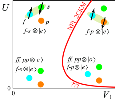
Figure 1: (Color online) Schematic ground-state $V_{1}$-$U$ phase diagram of model (1).Yashiki1 ; Yashiki2 There are two phases. One is the phase characterized by the parity-even ground state for small $V_{1}$, while the other is the odd-parity state for large $V_{1}$. Inside the each phase, the electron and also the phonon configurations crossover as $U$ varies. $|e\rangle(|o\rangle)$ represents the even (odd) parity phonon state. Between the two phases, there is a line of NFL fixed points for all the values of $U>0$ where the fixed point spectra of the NRGDaggoto ; Yashiki1 ; Yashiki2 are the same as those in magnetic 2CKM. In the figure, we depict characteristic configurations with the spin singlet in each region in the two phases. $f$-$s(p)$ indicates the spin-singlet state between $f$ and $s(p)$ electrons and $f\!f(pp)$ represents the double occupied state for the $f(p)$ electron.

II.2 Non-Abelian Bosonization

In this section, we map the original Hamiltonian to one in an effective one-dimensional continuous “radial” space with only left-moving conduction electron components, and we apply non-Abelian bosonization.Aff1 In this approach, the free electron part of the Hamiltonian (1) is written as

$$H_{0}=\frac{iv_{F}}{2\pi}\int dx\Big{[}s_{\sigma}^{\dagger}(x)\partial_{x}s_{\sigma}(x)+p_{\sigma}^{\dagger}(x)\partial_{x}p_{\sigma}(x)\Big{]},$$ (7)

where $x$ is the position in the one-dimensional space and $v_{F}$ is the Fermi velocity.

II.2.1 Conformal embedding: U(1)$\otimes$SU(2)${}_{2}\otimes$SU(2)₂

The Hamiltonian (7) consists of two flavors of conduction electrons $s$ and $p$ with the spin $j=1/2$. When we apply non-Abelian bosonization to this model, the simplest way of so called conformal embedding is to bosonize, global charge U(1), spin SU(2) and flavor SU(2) degrees of freedom.Aff2 ; Aff3 We set the one-dimensional system size as $[-l,l]$ and the bosonized Hamiltonian leads

$$H_{0} = \frac{\pi v_{F}}{l}\sum_{n}\Big{[}\frac{1}{8}:J_{n}J_{-n}:+\frac{1}{4}:{\bf J}_{n}\cdot{\bf J}_{-n}:$$ (8)

$$+\frac{1}{4}:{\bf F}_{n}\cdot{\bf F}_{-n}:\Big{]},$$

where $J_{n}$, ${\bf J}_{n}=(J_{n}^{x},J_{n}^{y},J_{n}^{z})$, and ${\bf F}_{n}=(F_{n}^{x},F_{n}^{y},F_{n}^{z})$ represent the charge, spin, and flavor (left moving) current operators in the Fourier space labeled by integers $n$, respectively, and $:A:$ is the normal ordering of operator $A$. $J_{n}$ satisfies the U(1) boson commutation relation, and ${\bf J}_{n}$ and ${\bf F}_{n}$ satisfy the SU(2)_k Kac-Moody algebra with the level $k=2$. This conformal embedding is suitable when the interactions consist of, for example, exchange interactions in the spin sector as in the case of the conventional two-channel Kondo problem.Aff2 ; Aff3 However, it is inconvenient for us, since there is no flavor SU(2) symmetry in the Hamiltonian (1).

II.2.2 Conformal embedding: SU(2)${}_{2}\otimes$SO(5)₂

As is well known, the symmetry in the 2CKM is higher than U(1)$\otimes$SU(2)$\otimes$SU(2), and it is SU(2)$\otimes$SO(5).Aff4 In the NRG studies of the Hamiltonian (1), SU(2)$\otimes$SO(5) symmetry is also realized along the line of the NFL fixed points.Yashiki1 ; Yashiki2 In this subsection, we clarify what SO(5) degrees of freedom are in the model (1).

First, we introduce the Nambu representation:

$$\bar{\Psi}(x) = [s^{\dagger}_{\uparrow}(x),-p^{\dagger}_{\uparrow}(x),p_{\downarrow}(x),s_{\downarrow}(x)],$$ (9)

$${\Psi}(x) = {}^{t}[s_{\uparrow}(x),-p_{\uparrow}(x),p^{\dagger}_{\downarrow}(x),s^{\dagger}_{\downarrow}(x)].$$ (10)

We find that the SO(5) “density” is given by using $\Psi(x)$ as

$$L^{ab}(x)=\sum_{\alpha=1}^{4}\sum_{\beta=1}^{4}\bar{\Psi}_{\alpha}(x)(\mathcal{L}^{ab})_{\alpha\beta}\Psi_{\beta}(x),$$ (11)

where ${\mathcal{L}^{ab}}\equiv\Gamma^{ab}/2$ with $1\leq a<b\leq 5$ are SO(5) generators and defined as 4 by 4 matrices as shown in Appendix A.1.Wu They define SO(5) rotations and satisfy the SO(5) commutation relation (42). There are ten generators in the SO(5) group, which are the adjoint representation, denoted by ${\bf 10}$. For later purposes, we define the 10-component vector ${\bf L}(x)$ as

$${\bf L}(x)\equiv(L^{12},L^{13},L^{14},L^{15},L^{23},L^{24},L^{25},L^{34},L^{35},L^{45}),$$ (12)

where $x$ dependence is omitted on the right-hand side of Eq. (12). We can bosonize ${\bf L}(x)$ and their Fourier components ${\bf L}_{n}$ satisfy the following SO(5)_k Kac-Moody algebra with the level $k=2$:hat1

$$[{L}^{ab}_{n},{L}^{cd}_{m}] = if^{ab,cd,ef}L^{ef}_{n+m}+\frac{nk}{2}\delta_{ac}\delta_{bd}\delta_{n+m,0}.$$ (13)

Here, $f^{ab,cd,ef}$ is the SO(5) structure constant and is given by Eqs. (41) and (42).

The Hamiltonian (7) is bosonized by using the conformal embedding SU(2)${}_{2}\otimes$SO(5)₂, leading to

$$H_{0}=\frac{\pi v_{F}}{l}\sum_{n}\Big{[}\frac{1}{4}:{\bf J}_{n}\cdot{\bf J}_{-n}:+\frac{1}{8}:{\bf L}_{n}\cdot{\bf L}_{-n}:\Big{]}.$$ (14)

Indeed, the central charge for the SO(5) sector is $c_{SO(5)}=5/2$ and that for the spin sector is $c_{s}=3/2$, leading to $c_{s}+c_{SO(5)}=4$ as it should be. This form (14) is used in a spin-3/2 dipole-octupole Kondo problem.hat1 There, $\Psi(x)$ corresponds to the spin-3/2 fermion operator and the SO(5) generators correspond to linear combinations of the spin-3/2 dipole and octupole operators, and the spin current ${\bf J}$ is replaced by the SU(2) axial charge current. Since, in the spin-3/2 model, quadrupole operators are classified as the SO(5) vector, i.e., the ${\bf 5}$ representation, we define the corresponding degrees of freedom in our model and they are given by

$$n^{a}(x)=\frac{1}{2}\sum_{\alpha=1}^{4}\sum_{\beta=1}^{4}\bar{\Psi}_{\alpha}(x)(\Gamma^{a})_{\alpha\beta}\Psi_{\beta}(x),$$ (15)

where $\Gamma^{a}$’s with $1\leq a\leq 5$ are 4 by 4 matrices defined in Appendix A.2. In the following, we use a five-component vector ${\bf n}(x)=(n^{1}(x),\cdots,n^{5}(x))$. Note that the spin eigenvalue of ${\bf n}(x)$ is $j=1$ and the z-component $j_{z}=0$, while $j=0$ for ${\bf L}(x)$. $j_{z}=\pm 1$ components of the ${\bf 5}$ representation ${\bf n}_{\pm}(x)$ can be constructed by applying the spin operators ${J}^{\pm}(x)={J}^{x}(x)\pm i{J}^{y}(x)$ to ${\bf n}(x)$. In total, 28 operators, ${\bf J}$, ${\bf L}$, ${\bf n}$, and ${\bf n}_{\pm}$, form a complete set of the conduction electron “density” operators in the sense of the Nambu representation.

It is also important to check the “independence” of the two sectors and we find, by direct calculations, $[L^{ab}(x),J^{\mu}(x^{\prime})]=0$, i.e., they are “independent.” The actual form of ${\bf L}(x)$ and ${\bf n}(x)$ is given in Table 1. It is clear that ${\bf L}(x)$ consists of charge, flavor, and spin-singlet pairing operators, while ${\bf n}(x)$ consists of spin-triplet pairing and a complex object of spin-flavor operators, see Appendix B. In terms of $L^{ab}_{n}$, the charge current $J_{n}$ and the flavor current ${\bf F}_{n}$ in Eq. (8) are related to $-L^{15}_{n}$, and $(-L^{34}_{n},L^{24}_{n},L_{n}^{23})$, respectively.

By using this conformal embedding, the free electron energy spectra $E_{0}$ are calculated via eigenvalues of the Casimir operators in the two sectors and are given byhat1

$$E_{0}=\frac{\pi v_{F}}{l}\Big{[}\frac{j(j+1)}{4}+\frac{C_{SO(5)}}{8}+m\Big{]}.$$ (16)

Here, $m$ is a non-negative integer, $m\geq 0$ and $C_{SO(5)}$ is the eigenvalue of the Casimir operator in the SO(5) sector. The eigenvalue depends on the irreducible representations and is given as $C_{SO(5)}=0$ for the identity ${\bf 1}$, $5/2$ for the spinor ${\bf 4}$, and $4$ for the vector ${\bf 5}$. Eigenstates with $m=0$ means that the eigenstate is a primary state, while those with $m\geq 1$ indicates that the states include particle-hole excitations and are classified as descendant states in the conformal tower characterized by a set of primary states.cft The SU(2)₂ Kac-Moody algebra restricts possible values of $j$ for the primary states in the spin sector. The spin $j$ of the primary states should be $0\leq j\leq k/2=1$.Aff2 The SO(5)₂ Kac-Moody algebra also restricts the number of primary states in the SO(5) sector, and, as shown in Appendix C, there are three primary states in the SO(5) sector: the identity ${\bf 1}$, the spinor ${\bf 4}$, and the vector ${\bf 5}$. Using Eq. (16), we can reproduce the free-electron spectra as shown in Table 2 (a).

Table 1: List of operators in the SO(5) sector. Each of irreducible representation is labeled by $(j_{j_{z}}$, dimension of the SO(5) group). Position index $x$ is omitted for ${\bf L}(x)$ and ${\bf n}(x)$ and the operator forms shown are those multiplied by a factor 2: $2{\bf L}(x)$, $2{\bf n}(x)$, $2{\bf L}_{I}$ and $2{\bf n}_{I}$. Each operator is labeled by the parity $P$, the axial charge eigenvalue $i$ and the z-component $i_{z}$, and the flavor $F$ (see, analysis in Sec. II.2.4). $i_{i_{z}}=1_{\pm 1}$ means that the operator is in linear combinations of $i_{z}=1$ and $-1$.

$(j_{j_{z}},{\rm SO(5)})$	label	operator form	$P$	$i_{i_{z}}$	$F$
(00,10)	$L^{12}$	$-s^{\dagger}_{\uparrow}s^{\dagger}_{\downarrow}+p^{\dagger}_{\uparrow}p^{\dagger}_{\downarrow}+{\rm h.c.}$	0	$1_{\pm 1}$	1
	$L^{13}$	$i(s^{\dagger}_{\uparrow}s^{\dagger}_{\downarrow}+p^{\dagger}_{\uparrow}p^{\dagger}_{\downarrow})+{\rm h.c.}$	0	$1_{\pm 1}$	0
	$L^{14}$	$-s^{\dagger}_{\uparrow}p^{\dagger}_{\downarrow}-p^{\dagger}_{\uparrow}s^{\dagger}_{\downarrow}+{\rm h.c.}$	1	$1_{\pm 1}$	0
	$L^{15}$	$-\sum_{\sigma}(s^{\dagger}_{\sigma}s_{\sigma}+p^{\dagger}_{\sigma}p_{\sigma})+2$	0	$1_{0}$	0
	$L^{23}$	$\sum_{\sigma}(s^{\dagger}_{\sigma}s_{\sigma}-p^{\dagger}_{\sigma}p_{\sigma})$	0	$1_{0}$	1
	$L^{24}$	$-i\sum_{\sigma}(s_{\sigma}^{\dagger}p_{\sigma}-p^{\dagger}_{\sigma}s_{\sigma})$	1	$0_{0}$	1
	$L^{25}$	$i(s^{\dagger}_{\uparrow}s^{\dagger}_{\downarrow}-p^{\dagger}_{\uparrow}p^{\dagger}_{\downarrow})+{\rm h.c.}$	0	$1_{\pm 1}$	1
	$L^{34}$	$-\sum_{\sigma}(s_{\sigma}^{\dagger}p_{\sigma}+p^{\dagger}_{\sigma}s_{\sigma})$	1	$1_{0}$	0
	$L^{35}$	$s^{\dagger}_{\uparrow}s^{\dagger}_{\downarrow}+p^{\dagger}_{\uparrow}p^{\dagger}_{\downarrow}+{\rm h.c.}$	0	$1_{\pm 1}$	0
	$L^{45}$	$i(s^{\dagger}_{\uparrow}p^{\dagger}_{\downarrow}+p^{\dagger}_{\uparrow}s^{\dagger}_{\downarrow})+{\rm h.c.}$	1	$1_{\pm 1}$	0
(10,5)	$n^{1}$	$i(s^{\dagger}_{\uparrow}p^{\dagger}_{\downarrow}+s^{\dagger}_{\downarrow}p^{\dagger}_{\uparrow})+{\ \rm h.c.}$	1	$1_{\pm 1}$	1
	$n^{2}$	$\sum_{\sigma}\sigma(s^{\dagger}_{\sigma}p_{\sigma}+p^{\dagger}_{\sigma}s_{\sigma})$	1	$0_{0}$	0
	$n^{3}$	$-i\sum_{\sigma}\sigma(s^{\dagger}_{\sigma}p_{\sigma}-p^{\dagger}_{\sigma}s_{\sigma})$	1	$1_{0}$	1
	$n^{4}$	$\sum_{\sigma}\sigma(s^{\dagger}_{\sigma}s_{\sigma}-p^{\dagger}_{\sigma}p_{\sigma})$	0	$0_{0}$	1
	$n^{5}$	$-s^{\dagger}_{\uparrow}p^{\dagger}_{\downarrow}-s^{\dagger}_{\downarrow}p^{\dagger}_{\uparrow}+{\ \rm h.c.}$	1	$1_{\pm 1}$	1
(00,10)	$L^{12}_{I}$	$\tau_{z}(f^{\dagger}_{\uparrow}f^{\dagger}_{\downarrow}+f_{\downarrow}f_{\uparrow})$	0	$1_{\pm 1}$	1
	$L_{I}^{13}$	$-i(f^{\dagger}_{\uparrow}f^{\dagger}_{\downarrow}-f_{\downarrow}f_{\uparrow})$	0	$1_{\pm 1}$	0
	$L_{I}^{14}$	$-\tau_{x}(f^{\dagger}_{\uparrow}f^{\dagger}_{\downarrow}+f_{\downarrow}f_{\uparrow})$	1	$1_{\pm 1}$	0
	$L_{I}^{15}$	$-(\sum_{\sigma}n_{f\sigma}-1)$	0	$1_{0}$	0
	$L_{I}^{23}$	$\tau_{z}(\sum_{\sigma}n_{f\sigma}-1)$	0	$1_{0}$	1
	$L_{I}^{24}$	$-\tau_{y}{\mathcal{P}}$	1	$0_{0}$	1
	$L_{I}^{25}$	$-i\tau_{z}(f^{\dagger}_{\uparrow}f^{\dagger}_{\downarrow}-f_{\downarrow}f_{\uparrow})$	0	$1_{\pm 1}$	1
	$L_{I}^{34}$	$\tau_{x}(\sum_{\sigma}n_{f\sigma}-1)$	1	$1_{0}$	0
	$L_{I}^{35}$	$-(f^{\dagger}_{\uparrow}f^{\dagger}_{\downarrow}+f_{\downarrow}f_{\uparrow})$	0	$1_{\pm 1}$	0
	$L_{I}^{45}$	$i\tau_{x}(f^{\dagger}_{\uparrow}f^{\dagger}_{\downarrow}-f_{\downarrow}f_{\uparrow})$	1	$1_{\pm 1}$	0
(00,5)	$n_{I}^{1}$	$-\tau_{y}(f^{\dagger}_{\uparrow}f^{\dagger}_{\downarrow}+f_{\downarrow}f_{\uparrow})$	1	$1_{\pm 1}$	1
	$n_{I}^{2}$	$\tau_{x}{\mathcal{P}}$	1	$0_{0}$	0
	$n_{I}^{3}$	$\tau_{y}(\sum_{\sigma}n_{f\sigma}-1)$	1	$1_{0}$	1
	$n_{I}^{4}$	$\tau_{z}{\mathcal{P}}$	0	$0_{0}$	1
	$n_{I}^{5}$	$-i\tau_{y}(f^{\dagger}_{\uparrow}f^{\dagger}_{\downarrow}-f_{\uparrow}f_{\downarrow})$	1	$1_{\pm 1}$	1

II.2.3 Local operators classified in a hidden SO(5) group

In this subsection, we will introduce local “flavor” degrees of freedom. Using them combined with ${\bf I}$, we will show that we can construct local SO(5) degrees of freedom in terms of local operators: $f$, $f^{\dagger}$, $b$, and $b^{\dagger}$ for small $U$.

In Ref. 21, it is shown that the energy spectra of small-cluster problems capture the essential aspect of the critical line obtained in the NRG calculations. Namely, there is a level crossing of the ground states of the $(j,i)=(0,1/2)$ sector. Here, $j(i)$ represents the eigenvalue of total spin (axial charge). Let us briefly explain their results in the following.

First, for large $V_{1}$, it is natural to consider a two-site problem, where $f$ and $p(0)$ electrons and $b$ are taken into account. For $U=0$, the Lang-Firsov transformationLang provides the exact solution of this problem. The ground state for $U=0$ is doubly degenerate. The two are two-electron states with the spin being singlet. This degeneracy is distinguished by the parity, i.e., one is an even-parity state $|\phi_{e}\rangle$ and the other is odd: $|\phi_{o}\rangle$. This degeneracy, however, is lifted by $U$, and for small but finite $U$, the ground state is the even-parity state with a small excitation gap to the odd-parity state. Importantly, in the low-energy states for $U=0$, the phonon $b$ appears only in the special combinations of the even- and odd-parity states:Yashiki2

$$|e\rangle = \cosh\Big{[}2\lambda(b-b^{\dagger})\Big{]}|0\rangle_{\rm ph},$$ (17)

$$|o\rangle = \sinh\Big{[}2\lambda(b-b^{\dagger})\Big{]}|0\rangle_{\rm ph}.$$ (18)

Here, $|0\rangle_{\rm ph}$ represents the vacuum of the phonon and $\lambda=-V_{1}/\Omega$. The other phonon states are in higher energy above $\Omega$, and thus do not play important roles.

The three-site problem, where $f$, $p(0)$, and $s(0)$ electrons and the phonons $b$ are taken into account, exhibits a qualitatively correct phase diagram, if we see the sector of two-electron or four-electron states, i.e., $i=1/2$ states. For small $V_{1}$, the ground state of the two-electron sector is an even-parity spin-singlet state, $|\phi^{\prime}_{e}\rangle\sim|\phi_{e}\rangle$, while for large $V_{1}$ the ground state changes to an odd-parity spin-singlet state $|\phi^{\prime}_{o}\rangle\sim|\phi_{o}\rangle$. The same is true in the four-electron sector, and we denote them as $|\psi^{\prime}_{e}\rangle$ and $|\psi^{\prime}_{o}\rangle$. Their spin eigenvalues are also $j=0$. Thus, there is a line where a level crossing occurs. Along the level-crossing line, the energies of these four states—$|\phi^{\prime}_{e}\rangle$, $|\phi^{\prime}_{o}\rangle$, $|\psi^{\prime}_{e}\rangle$, and $|\psi^{\prime}_{o}\rangle$—coincide and they form an SO(5) spinor, $\bf 4$ representation, in the SO(5) group. With regard to the $(i,j)=(0,1/2)$ sector, there are quasi-degenerate states with even and odd parity that originate in the ground states for the two-site problem with one electrons in the $s$-orbital. One is an SO(5)-singlet, while the other is one of the states in the ${\bf 5}$ representation.

Our assumption on the phonon degrees of freedom for small $U$ is that the only two states, such as $|e\rangle$ and $|o\rangle$, which are solely constructed by the phonon part, are important in the low-energy properties along the critical line. Indeed, this is valid in the limit of $U=0$, since the first excited state lies at $\Omega$, and thus it does not play any role in the low-energy physics.Yashiki2 Then, we can construct “flavor” operators characterized by the Pauli matrices in these two bases and we denote them as $\tau_{x},\tau_{y}$, and $\tau_{z}$, identifying the even-parity state as $|\!\!\Uparrow\rangle$ and the odd-parity state as $|\!\Downarrow\rangle$. The level crossing in the three-site problem is described by the presence of a term $\propto(U-U_{c})\tau^{z}$ while fixing other parameters, where $U_{c}$ is the level-crossing value of $U$. Note that, for $U>0$, there is always a finite gap between the even and odd ground states in the (0,1/2) sector, since the gap arises mainly from the fact that the two are classified in a different irreducible representation and thus have generally different energies.

Another local degree of freedom is the $f$ operator part. We consider quadratic operators in terms of $f_{\sigma}$ and $f^{\dagger}_{\sigma}$. Possible linear combinations are the spin ${\bf S}$ and the axial charge ${\bf I}$; see Eqs. (2), (3) and (4). Since the SO(5) sector is nonmagnetic, we consider the $f$-electron part of the axial charge, ${\bf I}$, in detail.

${\bf I}$ satisfies the SU(2) commutation relations, and thus, the eigenvalue of ${\bf I}^{2}$ is $i(i+1)$ with $i=0$ or $1/2$. When $I_{\alpha}$ acts on an $i=0$ subspace $f^{\dagger}_{\sigma}|0\rangle$, where $|0\rangle$ is the vacuum of the $f$-electrons, $I_{\alpha}f^{\dagger}_{\sigma}|0\rangle=0$. Because of this property, the operation of $I_{\alpha}$ is automatically projected on an $i=1/2$ subspace, $|0\rangle$ and $f_{\uparrow}^{\dagger}f_{\downarrow}^{\dagger}|0\rangle$. This is very important in the derivation of local SO(5) degrees of freedom below, since the algebra of $\tilde{I}_{\alpha}\equiv 2I_{\alpha}$ is very similar to that of the Pauli matrices. Indeed, $\tilde{I}_{\alpha}$’s satisfy

$$[\tilde{I}_{\alpha},\tilde{I}_{\beta}] = 2i\epsilon_{\alpha\beta\gamma}\tilde{I}_{\gamma},$$ (19)

$$\{\tilde{I}_{\alpha},\tilde{I}_{\beta}\} = 2{\mathcal{P}}\delta_{\alpha\beta},$$ (20)

$${\mathcal{P}} \equiv \tilde{I}_{x}^{2}=\tilde{I}_{y}^{2}=\tilde{I}_{z}^{2}=2n_{f\uparrow}n_{f\downarrow}-\tilde{I}_{z},$$ (21)

$$\tilde{I}_{\alpha}{\mathcal{P}} = {\mathcal{P}}\tilde{I}_{\alpha}=\tilde{I}_{\alpha},$$ (22)

where $\mathcal{P}$ is the projection operator onto the $i=1/2$ subspace and is alternatively given by ${\mathcal{P}}=4{\bf I}^{2}/3$.

Now, let us first introduce an SO(5) vector, i.e., the ${\bf 5}$ representation ${\bf n}_{I}$:

$${\bf n}_{I}=\frac{1}{2}(\tilde{I}_{x}\tau_{y},{\mathcal{P}}\tau_{x},\tilde{I}_{z}\tau_{y},{\mathcal{P}}\tau_{z},-\tilde{I}_{y}\tau_{y}).$$ (23)

Note that ${\bf n}_{I}$ is a spin-singlet operator unlike ${\bf n}(x)$ of the conduction electron with the spin being triplet, and ${\bf n}_{I}$ includes $\tilde{I}_{\alpha}$ in all the components, which means ${\bf n}_{I}$ acts on the $i=1/2$ subspace. At this stage, it is not proved that ${\bf n}_{I}$ transforms as an SO(5) vector, since we have not defined any local SO(5) generator. Thus, let us define a trial local SO(5) generators, ${\bf 10}$, via Eq. (44), $2L_{I}^{ab}\equiv[2n^{a}_{I},2n^{b}_{I}]/(2i)$, and we obtain

$${\bf L}_{I} = \frac{1}{2}(-\tilde{I}_{x}\tau_{z},-\tilde{I}_{y},\tilde{I}_{x}\tau_{x},-\tilde{I}_{z},\tilde{I}_{z}\tau_{z},-{\mathcal{P}}\tau_{y},-\tilde{I}_{y}\tau_{z},$$ (24)

$$\ \ \tilde{I}_{z}\tau_{x},\tilde{I}_{x},\tilde{I}_{y}\tau_{x}).$$

The trial SO(5) generators $L_{I}^{ab}$’s, indeed, satisfy the SO(5) commutation relations (42): $[L_{I}^{ab},L_{I}^{cd}]=-i(\delta_{bc}L_{I}^{ad}-\delta_{ac}L_{I}^{bd}-\delta_{bd}L_{I}^{ac}+\delta_{ad}L_{I}^{bc})$. Thus, $L^{ab}_{I}$ denotes the SO(5) generators that we seek. We can also confirm that the commutation relation between ${2\bf L}_{I}$ and ${2\bf n}_{I}$ is similar to Eq. (45), $[2n_{I}^{a},2L_{I}^{bc}]=-i({\rm sgn}(c-a)\delta_{ab}n_{I}^{c}+{\rm sgn}(b-a)\delta_{ac}n_{I}^{b})$ i.e., ${\bf n}_{I}$ is the ${\bf 5}$ representation of the local SO(5) group defined by ${\bf L}_{I}$.

Finally, we note that the four states

$${}^{t}(|\!\!\Downarrow\rangle,-|\!\!\Uparrow\rangle,-f^{\dagger}_{\uparrow}f^{\dagger}_{\downarrow}|\!\!\Uparrow\rangle,f^{\dagger}_{\uparrow}f^{\dagger}_{\downarrow}|\!\!\Downarrow\rangle)$$ (25)

transform as an SO(5) spinor, ${\bf 4}$ representation. This can be checked by applying ladder operators in the SO(5) group listed in Appendix C.

II.2.4 Exchange interactions

So far, we have analyzed how SO(5) degrees of freedom appear in the free part of the Hamiltonian (7) and what local SO(5) operations for small $U$ are. In this subsection, we phenomenologically discuss possible and/or impossible interactions under the SU(2)$\otimes$SO(5) symmetry, which are closely related to two fusions introduced in Sec. II.2.5. We show two possible exchange interactions but they are not the “microscopic” effective Hamiltonian of (1). They should be regarded as one of the effective interactions for the coarse-grained system.

The simplest invariant form under SU(2)$\otimes$SO(5) symmetry is exchange interactions between the impurity and the conduction electron component at the origin $x=0$. Spin-spin exchange interactions are evidently possible under SU(2)$\otimes$ SO(5) symmetry:

$$H_{\rm s}=J{\bf S}\cdot{\bf J}(0),$$ (26)

with $J$ being the coupling constant. This term preserves the symmetry of the original Hamiltonian (1), and can be regarded as the effective interactions after integration of the phonon and ${\bf I}^{2}=3/4$ sector.

Similarly, exchange interactions in the SO(5) sector are also possible:

$$H_{\rm SO(5)}=K{\bf L}_{I}\cdot{\bf L}(0).$$ (27)

Here, $K$ denotes the coupling constants. This can be obtained after integrating the sector of ${\bf I}^{2}=0$. Note that due to the mismatch in the eigenvalue of the spin $j$, a term ${\bf n}_{I}\cdot{\bf n}(0)$ cannot exist, when the spin SU(2) or time reversal symmetry is present.

In order to understand that the interaction (27) respects the original symmetry of the Hamiltonian (1), namely the charge SU(2) symmetry, the spin SU(2) symmetry, and the $Z_{2}$ symmetry, we expand ${\bf L}_{I}\cdot{\bf L}(0)$ in the fermion representations:

$${\bf L}_{I}\cdot{\bf L}(0) = \frac{1}{2}\Big{\{}\Big{[}I_{+}\Big{(}s_{\downarrow}(0)s_{\uparrow}(0)+p_{\downarrow}(0)p_{\uparrow}(0)\Big{)}+{\rm h.c.}\Big{]}$$

$$+ I_{z}\Big{[}\sum_{\sigma}\Big{(}s^{\dagger}_{\sigma}(0)s_{\sigma}(0)+p^{\dagger}_{\sigma}(0)p_{\sigma}(0)\Big{)}-2\Big{]}\Big{\}}$$

$$+ \frac{1}{2}\tau_{z}\Big{\{}\Big{[}I_{+}\Big{(}s_{\downarrow}(0)s_{\uparrow}(0)-p_{\downarrow}(0)p_{\uparrow}(0)\Big{)}+{\rm h.c.}\Big{]}$$

$$+ I_{z}\sum_{\sigma}\Big{[}s^{\dagger}_{\sigma}(0)s_{\sigma}(0)-p^{\dagger}_{\sigma}(0)p_{\sigma}(0)\Big{]}\Big{\}}$$

$$- \frac{1}{2}\tau_{x}\Big{\{}\Big{[}I_{+}\Big{(}p_{\downarrow}(0)s_{\uparrow}(0)+s_{\downarrow}(0)p_{\uparrow}(0)\Big{)}+{\rm h.c.}\Big{]}$$

$$+ I_{z}\sum_{\sigma}\Big{[}p^{\dagger}_{\sigma}(0)s_{\sigma}(0)+{\rm h.c.}\Big{]}\Big{\}}$$

$$+ \frac{i}{4}\tau_{y}{\mathcal{P}}\sum_{\sigma}\Big{[}s^{\dagger}_{\sigma}(0)p_{\sigma}(0)-{\rm h.c.}\Big{]},$$

$$\equiv {\bf I}\cdot\Big{[}{\bf I}(0)+\tau_{z}{\bf I}^{\prime}(0)-\tau_{x}{\bf I}^{\prime\prime}(0)\Big{]}-\frac{1}{2}\tau_{y}{\mathcal{P}\mathcal{D}}(0).$$

Here, ${\bf I}(0)$ is the local axial charge for the conduction electrons. As shown in Appendix B, ${\bf I}^{\prime}(0)$ is the local longitudinal-flavor axial charge, while ${\bf I}^{\prime\prime}(0)$ is the local transverse-flavor axial charge. All three transform as vectors under the charge SU(2) rotations, while ${\mathcal{D}}(0)$ is invariant; see Appendix B. Since ${\bf I}$ transforms as a vector and $\mathcal{P}$ is invariant under the charge SU(2) rotations, Eq. (LABEL:II) is invariant under the charge SU(2) operations. As for the parity, ${\bf I}$, $\tau_{z}$, $\mathcal{P}$, ${\bf I}(0)$, and ${\bf I}^{\prime}(0)$ are even parity, while $\tau_{x}$, $\tau_{y}$, ${\bf I}^{\prime\prime}(0)$ and ${\mathcal{D}}(0)$ are odd parity. Thus, Eq. (LABEL:II) is even parity, i.e., invariant under the inversion operation. Finally, since all the terms are spin singlet, Eq. (LABEL:II) is invariant under the spin SU(2) operations. These facts confirm that ${\bf L}(0)\cdot{\bf L}_{I}$ is invariant under the original symmetry.

In addition to the symmetry of the Hamiltonian (1), the exchange interactions (26) and (27) have an additional flavor symmetry. The flavor symmetry operation is defined as $|\!\!\Uparrow\rangle\!\leftrightarrow\!|\!\!\Downarrow\rangle$ and $s_{\sigma}\!\leftrightarrow\!p_{\sigma}$. There are two kinds of operators in terms of the flavor symmetry: even or odd. Even-flavor operators are denoted by $F=0$, while odd ones are denoted by $F=1$ in Table 1. The values of $F$ are related to the eigenvalues of the flavor transformation as $(-1)^{F}$. As will be investigated in Sec. II.2.7, this symmetry breaking drives the system away from the critical line.

Note that there is also flavor SU(2) symmetry in Eq. (27), when we define the local flavor operators as ${\bf F}_{I}\equiv$$(-L_{I}^{34},L_{I}^{24},L_{I}^{23})$. It is also important to note that the phonon flavor operator $\vec{\tau}$ cannot directly couple with conduction electron flavor ${\bf F}_{n}$ in the presence of the charge SU(2) symmetry. This means that simple flavor-exchange Kondo couplings

$$H_{\rm flavor}=J_{f}\vec{\tau}\cdot{\bf F}(0)$$ (30)

never appear under the presence of particle-hole symmetry and $H_{\rm flavor}$ is absent also away from the critical line. In this sense, even away from the critical line, the screening processes of impurity degrees of freedom in the model (1) with the charge SU(2) symmetry are not the same as those in the flavor Kondo model such as in the two-level systemsCox . Away from the critical line with the charge SU(2) symmetry, a possible form in the (phonon-only) flavor interaction is Ising like:

$$H_{\rm flavor}^{xy}=(J^{x}_{f}\tau_{x}+J^{y}_{f}\tau_{y})F^{y}(0)=(J_{f}^{x}\tau_{x}+J_{f}^{y}\tau_{y}){\mathcal{D}}(0).$$ (31)

This is because only $\mathcal{D}(0)=F^{y}(0)=L^{24}(0)$ is a charge and also a spin SU(2) singlet operator in the “local density” form constructed by the conduction electron operators. Since this is an Ising interaction, when only this term is present, nonmagnetic “Kondo effects” never occur.

Table 2: (a) Spectra of the free Hamiltonian (7) for a non-degenerate ground state. (b) The spectra at the NFL fixed point. The energy $E_{0}$ and $E$ are measured in the unit of $\pi v_{F}/l$. (c) Operator contents at the NFL fixed point. $\Delta$ is the scaling dimension of the operators labeled by the quantum numbers $j$ and the dimension of the irreducible representation in the SO(5) group.

(a)			(b)			(c)
$\ \ j\ \ \$	SO(5)	$\ \ \ E_{0}\ \ \$	$\ \ j\ \ \$	SO(5)	$\ \ \ E\ \ \$	$\ \ j\ \ \$	SO(5)	$\ \ \ \Delta\ \ \$
0	${\bf 1}$	$0$	$\frac{1}{2}$	${\bf 1}$	0	0	${\bf 1}$	0
$\frac{1}{2}$	${\bf 4}$	$\frac{1}{2}$	0	${\bf 4}$	$\frac{1}{8}$	0	${\bf 5}$	$\frac{1}{2}$
1	${\bf 5}$	$1$	$\frac{1}{2}$	${\bf 5}$	$\frac{1}{2}$	1	${\bf 1}$	$\frac{1}{2}$
0	${\bf 10}$	$1$	1	${\bf 4}$	$\frac{5}{8}$	$\frac{1}{2}$	${\bf 4}$	$\frac{1}{2}$
1	${\bf 1}$	$1$	$\frac{3}{2}$	${\bf 1}$	$1$	$\frac{1}{2}$	${\bf 4}$	$\frac{1}{2}$
$\frac{3}{2},\frac{1}{2}$	${\bf 4}$	$\frac{3}{2}$	$\frac{1}{2}$	${\bf 10}$	$1$	1	${\bf 5}$	$1$
$\frac{1}{2}$	${\bf 16}$	$\frac{3}{2}$	$\frac{1}{2}$	${\bf 1}$	$1$	0	${\bf 10}$	1

II.2.5 Fusions

In this subsection, we introduce two different fusionsAff2 ; Aff3 that derive the spectra obtained in the NRG calculations along the critical line.Daggoto ; Yashiki1 ; Yashiki2 Although, due to the fact that the model (1) is not described by a simple exchange Hamiltonian, we cannot carry out a direct impurity absorption as in exchange models such as multi-channel and spin-3/2 multipolar Kondo problemsAff2 ; Aff3 ; hat1 , we will show that two fusions indeed derive the same NFL spectra as in the 2CKM.

The first candidate of the fusion is spin-$1/2$ fusion in the SU(2)₂ sector, which is the same as the case of 2CKMAff2 ; Aff3 , leading to the NFL spectra shown in Table 2 (b). This fusion is physically natural and easy to understand, when we consider the process from large $U$ limit, since for large $U$ the relevant operator is expected to be the spin ${\bf S}$.

We find that there is an alternative way to derive the same NFL spectra, i.e., SO(5) spinor ${\bf 4}$ fusion:hat1 ${}^{t}(|\!\!\Downarrow\rangle,-|\!\!\Uparrow\rangle,-f^{\dagger}_{\uparrow}f^{\dagger}_{\downarrow}|\!\!\Uparrow\rangle,f^{\dagger}_{\uparrow}f^{\dagger}_{\downarrow}|\!\!\Downarrow\rangle)$. Since primary states in the SO(5)₂ sector are ${\bf 1}$, ${\bf 4}$, or ${\bf 5}$, the fusion rule is ${\bf 1}\to{\bf 4}$, ${\bf 4}\to{\bf 1}\oplus{\bf 5}$, and ${\bf 5}\to{\bf 4}$. These are obtained by discarding ${\bf 10}$ and ${\bf 16}$ representations in the SO(5) direct products: ${\bf 4}\otimes{\bf 4}={\bf 1}\oplus{\bf 5}\oplus{\bf 10}$ and ${\bf 5}\otimes{\bf 4}={\bf 4}\oplus{\bf 16}$. Indeed, this fusion rule generates the same low-energy spectra as the spin-1/2 fusion, as shown in Table 2(b).

As for double fusionsAff3 of spin $1/2$ and SO(5) ${\bf 4}$, the two different fusions lead to the identical operator contentLud ; hat1 shown in Table 2 (c). All the operators in Table 2 (c) that satisfy the SU(2)$\otimes$SO(5) symmetry can be present along the critical line. We expect that, for large $U$, the dominant leading irrelevant operator is in the spin sector, while for small $U$, it is in the SO(5) sector, since ${\bf S}$ is not active for small $U$.

Now, one might wonder what the difference between the two fusions is. We consider that these two are simply equivalent. In order to understand this, we show an example of this kind of situation in an impurity Anderson model, when the Coulomb interaction $U$ varies from $\infty$ to $0$ while maintaining particle-hole symmetry.

As is well known, the ground-state spectra of the Anderson model from the strong to the weak coupling regime are the same as those in the Kondo model with the charge quantum number being shifted. The spectra in the Kondo model are obtained by a spin-1/2 fusion via direct spin absorption.Aff1 Alternatively, the same spectra can be obtained by an axial charge $i=1/2$ fusion, i.e., a $\pi/2$ phase shift. In the Anderson model, both spin and charge degrees of freedom are present. When only exchange-type interactions are considered in the context of the coarse-grained Hamiltonian, there are two types of such interactions: $J_{s}{\bf S}\cdot{\bf J}(0)$ and $J_{c}{\bf I}\cdot{\bf{I}}(0)$. Here ${\bf J}(0)$ and ${\bf I}(0)$ represent the spin and axial charge current for conduction electrons, respectively. For large $U$, only the sector with ${\bf I}^{2}=0$ is relevant. Then, the spin-spin exchange coupling describes the low-energy physics, and thus the model reduced to the Kondo model. For small $U$, the charge-charge exchange interaction $J_{c}$ becomes compatible with the spin-spin exchange interaction $J_{s}$.

Now, one can realize that there are similarities between the Anderson model and the present one; $J_{s}$ corresponds to $J$ in Eq. (26) and $J_{c}$ to $K$ and ${\bf I}(0)({\bf I})$ to ${\bf L}(0)({\bf L}_{I})$ in Eq. (27). As for the fusion process, the axial charge fusion, i.e., the $\pi/2$ phase shift, in the Anderson model corresponds to the SO(5)-${\bf 4}$ fusion in the present model.

The spin-1/2 and SO(5)-${\bf 4}$ fusions introduced above are equivalent in the sense that the spin-1/2 fusion and the $\pi/2$ phase shift are equivalent in the Kondo or Anderson model. Our answer to the question “what is going on for small $U$?”, which is the main motivation in this paper, is that the NFL spectra of 2CKM can be obtained via the nonmagnetic SO(5)-${\bf 4}$ fusion, and thus, we can interpret the low-energy physics for small $U$ as the nonmagnetic SO(5) Kondo effects in the same way that the conventional Kondo effects can be interpreted as the strong potential scattering with the phase shift $\pi/2$. Of course, one can still interpret it as a magnetic one but the SO(5)-$\bf 4$ fusion is much better for understanding the physics for small $U$, since what makes the low-energy physics for small $U$ different from that for the Kondo regime is the nonmagnetic degrees of freedom. Indeed, as will be shown in Sec. III, the residual interactions around the NFL fixed point for small $U$ are governed by the operators in the SO(5) sector rather than those in the spin sector.

II.2.6 Leading irrelevant operators

Low-temperature thermodynamic properties are governed by leading irrelevant operators around the fixed point. In the Kondo regime, i.e., for large $U$, the leading irrelevant operator should be in the spin sector, and it is ${\bf J}_{-1}\cdot\vec{\phi}_{s}$, with ${\vec{\phi}}_{s}$ being spin-SU(2) primary fields with the dimension $\Delta=1/2$ and the quantum numbers $(j,{\rm SO(5)})=(1,{\bf 1})$ in Table 2 (c). In total, the dimension of this operator is $3/2$. In the presence of this operator, it is well knownAff2 ; Aff3 that the impurity contribution to the specific heat $C$ is proportional to $-T\ln T$, and the magnetic susceptibility $\chi_{s}$ diverges logarithmically $\chi_{s}\sim-\ln T$ at low temperatures.

For small $U$, we expect that the operator in the spin sector does not play an important role, and thus, operators in the SO(5) sector dominate. Then, the situation is analogous to the spin-3/2 dipole-octupole Kondo model.hat1 Since the first descendants of primary fields $\vec{\phi}_{\bf 5}$ with $(j,{\rm SO(5)})=(0,{\bf 5})$ and $\Delta=1/2$ in Table 2 (c), ${\bf L}_{-1}\vec{\phi}_{\bf 5}$, cannot form an SO(5) singlet, the leading irrelevant operator is the energy-momentum tensor in the SO(5) sector at the impurity site :${\bf L}(0)\cdot{\bf L}(0)$:. The leading dimension of this operator is $2$, i.e., the “Fermi liquid” like interaction.Aff1 This readily indicates that the low-temperature impurity specific heat $C\propto T$. As investigated in Ref. 34, the susceptibilities of the SO(5) vector ${\bf 5}$, $\vec{\phi}_{\bf 5}$, diverge logarithmically $\sim-\ln T$, indicating the divergence of the susceptibility of ${\bf n}_{I}$. The susceptibility of the SO(5) generators is independent of $T$ at low temperatures, since the dimension of the $(0,{\bf 10})$ operator in Table 2 (c) is $\Delta=1$. Thus, the susceptibilities of ${\bf L}_{I}$ are Fermi liquid like. We call these behaviors SO(5) NFL hereafter.

Here, we notice that the SO(5) vector in our model corresponds to $\tau_{y}I_{\alpha}$ and $\tau_{\beta}\mathcal{P}$ with $\alpha=x,y,\ {\rm or}\ z$ and $\beta=x,\ {\rm or}\ z$, see Table 1 and Eq. (23). Physically, these operators correspond to bipolaron fluctuations, which are coupled fluctuations of the flavor and the axial charge. In the original variables $b$ and $b^{\dagger}$, $\tau_{x}\pm i\tau_{y}$ are, roughly speaking, related to $b$ and $b^{\dagger}$.

In principle, there exist both terms ${\bf J}_{-1}\cdot\vec{\phi_{s}}$ and ${\bf L}(0)\cdot{\bf L}(0)$ for general values of $U$, since the original interaction is in complex form of the spin and SO(5) degrees of freedom and also terms that cannot be described by exchange forms. What varies as a function of parameters, e.g., $U$ along the critical line, is the coefficients of these operators in the effective Hamiltonian near the fixed point. Such a situation is represented by the following residual effective Hamiltonian:

$$\delta H_{{\rm eff}}=\lambda_{s}{\bf J}_{-1}\cdot\vec{\phi}_{s}+\lambda_{L}{\bf L}_{-1}\cdot{\bf L}_{-1},$$ (32)

where $\lambda_{s}$ and $\lambda_{L}$ depend on microscopic parameters such as $U$, $V_{0}$, and $V_{1}$. We have retained the leading term of ${\bf L}(0)\cdot{\bf L}(0)$ in the second term in Eq. (32) and we have not included a term ${\bf J}_{-1}\cdot{\bf J}_{-1}$, which has the dimension 2, since it is sufficient to include only the leading irrelevant operators in each of the sectors in the following analysis. As we investigated above, the relative magnitude of the two terms varies, and the first term is dominant in the Kondo regime, while the second one prevails in the weak coupling regime.

An interesting crossover is expected especially in the impurity contributions to specific heat $C$. Since two sectors are decoupled, $C$ is the sum of the contribution of each sector:Aff1 ; Aff3

$$C=-\gamma_{s}T\ln\Big{(}\frac{T}{T_{s}}\Big{)}+\gamma_{L}T.$$ (33)

Here, $T_{s}$ is a dynamically generated energy scale in the spin sector, which is proportional to the Kondo temperature in the Kondo regime. The parameter $\gamma_{s}(\gamma_{L})$ is proportional to $\lambda_{s}^{2}(\lambda_{L})$.Aff1 ; Aff3 As analyzed by Johannesson et al.,2cam $\lambda_{s}^{2}\sim 1/T_{s}$ and $\lambda_{L}\sim 1/T_{L}$, where $T_{L}$ is the “Kondo temperature” for the SO(5) sector. The crossover temperature $T^{*}$ can be defined by the temperature where the magnitudes of the two terms in Eq. (33) are equal, and is given by

$$T^{*}=T_{s}\exp\Big{(}-\frac{\gamma_{L}}{\gamma_{s}}\Big{)}.$$ (34)

For $T<T^{*}$, the specific heat due to the spin sector dominates, and thus, $C/T$ diverges logarithmically. However, for sufficiently small $U$, $\gamma_{L}/\gamma_{s}\sim T_{s}/T_{L}\gg 1$, thus, $T^{*}$ is never reached in a realistic temperature range and $C/T$ stays constant at low temperatures. This is a marked contrast between the NFL in the 2CKM and the SO(5) NFL.

Finally, let us comment on the “secondary-diverging” susceptibility in each of the parameter regime. Even for large $U$, the susceptibility of $\vec{\phi}_{\bf 5}$, indeed, diverges logarithmically. We call this divergence ”secondary”, since the coefficient of this part is expected to be very small for large $U$:2cam $\sim-[\ln(T/T_{L})]/T_{L}$ with $T_{L}\sim U/2$. The same is true for the spin susceptibility for small $U$. There, the system is in the valence fluctuation regime and the spin susceptibility is $\sim-[\ln(T/T_{s})]/T_{s}$ with $T_{s}$ proportional to the hybridization width.

II.2.7 Stability of the fixed points

In this subsection, we investigate the stability of the NFL fixed point derived in Sec. II.2.6 against various perturbations.

First, we investigate symmetry breaking fields. In Table 2 (c), there are SO(5)-${\bf 5}$ primary fields $\vec{\phi}_{\bf 5}$ with the dimension $\Delta=1/2$. Thus, when the SO(5) symmetry is broken, a term $\vec{h}_{\bf 5}\cdot\vec{\phi}_{{\bf 5}}$ appears in the effective Hamiltonian, which is relevant, and thus the NFL fixed point is unstable against this perturbation. Practically speaking, the SO(5) symmetry-breaking field $\vec{h}_{\bf 5}$ includes the inversion symmetry-breaking field and the flavor (even-odd) symmetry-breaking one.

In the presence of the inversion symmetry breaking field, $(\vec{\phi}_{\bf 5})_{2}$ with the quantum number $(j,i,P,F)=(0,0,1,0)$ appears in the effective Hamiltonian. Here $(\vec{\phi}_{\bf 5})_{i}$ represents the $i$th field in the five component vector $\vec{\phi}_{\bf 5}$. With regard to the flavor symmetry breaking field, $(\vec{\phi}_{\bf 5})_{4}$ with $(j,i,P,F)=(0,0,0,1)$ appears in the effective Hamiltonian. The Hamiltonian (1) has inversion symmetry, while the flavor symmetry is higher than that of the original Hamiltonian (1) and is realized only along the critical line. Thus, $(\vec{\phi}_{\bf 5})_{2}$ cannot appear even away from the critical line, while $(\vec{\phi}_{\bf 5})_{4}$ can appear away from the critical line and $(\vec{h}_{\bf 5})_{4}(\vec{\phi}_{\bf 5})_{4}$ is the perturbation that makes the NFL fixed points unstable. This flavor symmetry breaking causes the energy difference between $|\!\!\Uparrow\rangle$ and $|\!\!\Downarrow\rangle$. The flavor symmetry breaking is, indeed, consistent with the spectra in the NRG and in the small clusters as analyzed in Sec. II.2.3.

Another relevant field is the magnetic field $h$, since there is an SO(5)-singlet and spin-1 primary fields $\vec{\phi}_{s}$ in Table 2 (c) with $\Delta=1/2$, which couple with $h$. This is the same as in the 2CKMAff4 and we do not discuss it in detail.

Finally, particle-hole asymmetry is marginal, since the operator with $(j,i_{i_{z}},P,F)=(0,1_{0},0,0)$ is classified in $[j,{\rm SO(5)}]=(0,{\bf 10})$ and the dimension is $\Delta=1$ in Table 2 (c). This operator breaks the SO(5) symmetry. It is well known that the potential scattering $VI_{z}(0)$ is absorbed in phase shiftsCox , and thus, the NFL properties are not affected except for the specific heat for small $U$, as we discuss below. When particle-hole symmetry is broken by charge-conserved perturbations such as $VI_{z}(0)$, in addition to (32) with anisotropic exchange interactions in the SO(5) sector [see, Eq. (36)], anisotropic flavor exchange interactions are allowed to appear, leading to the additional residual interactions,

$$\delta H_{\rm eff}^{f}\sim g_{x}L_{-1}^{34}(\vec{\phi}_{\bf 5})_{2}+g_{y}L_{-1}^{24}(\vec{\phi}_{\bf 5})_{3}+g_{z}L_{-1}^{23}(\vec{\phi}_{\bf 5})_{4}.$$ (35)

Here, $(-L^{34}_{-1},L^{24}_{-1},L^{23}_{-1})={\bf F}_{-1}$ is the flavor current operator defined in Sec. II.2.2 and $g_{i}(i=x,y,\ {\rm or}\ z)$ is constant proportional to the symmetry breaking field $\sim V$. Note that this form is not SO(5) invariant. However, it is still invariant under the inversion and the spin SU(2) operations, and also the total charge is conserved. Since the scaling dimension of (35) is $\Delta=3/2$, the impurity contribution of the specific heat of this term is similar to that of the spin sector in Eq. (33).

Second, we investigate exchange anisotropies in the spin and the SO(5) sectors. The irrelevance of the spin exchange anisotropy is explained in the same way as in the case of the magnetic 2CKM.Aff4 As for the exchange anisotropy in the SO(5) sector, when the anisotropy exists, the isotropic effective interaction $K{\bf L}_{I}(0)\cdot{\bf L}(0)$ is replaced,

$$K{\bf L}_{I}\cdot{\bf L}(0) \to K{\bf L}_{I}\cdot{\bf L}(0)+\delta K^{\prime}\tau_{z}{\bf I}\cdot{\bf I}^{\prime}(0)$$ (36)

$$-\delta K^{\prime\prime}\tau_{x}{\bf I}\cdot{\bf I}^{\prime\prime}(0)-\frac{1}{2}\delta K^{\prime\prime\prime}\tau_{y}{\mathcal{P}\mathcal{D}}(0),\ \ \ \$$

where $\delta K^{\prime}$, $\delta K^{\prime\prime}$ and $\delta K^{\prime\prime\prime}$ are the deviations from the isotropic interactions. Note that Eq. (36) is charge-SU(2) invariant. This anisotropy generates residual interactions such as $L^{ab}_{-1}L^{ab}_{-1}$ with some sets of $ab$. This operator has dimension $2$, i.e., it is irrelevant.

III Numerical Renormalization Group Results

In this section, we examine the crossover from the SO(5) NFL to the NFL in the magnetic 2CKM as $U$ increases along the critical line by using Wilson’s NRG.nrg One of the advantage in using NRG is that we can obtain information about the scaling dimensions $\Delta$ of leading irrelevant operators around fixed points by analyzing spectra obtained in NRG.zarand ; koga The details of the NRG method are explained in a previous paper.Yashiki2 Here, we will analyze variations of NRG spectra along the critical line. A detailed analysis of physical quantities will be reported elsewhere.UnpublishHat

In this section, we will show data for three different parameters: large $U=0.8\tilde{D}$, small $U=0.02\tilde{D}$, and intermediate $U=0.2\tilde{D}$. Here, $\tilde{D}$ is related to half of the band width $D$ of conduction electrons for both $s$ and $p$ bands as $\tilde{D}=D(\Lambda+1)/(2\Lambda)$, and the Fermi energy is at the middle of the band. Here, $\Lambda$ is a discretization parameter in NRG and we use $\Lambda=3$. For each value of $U$, we tune the hybridization $V_{1}$ to realize the NFL fixed point, while $V_{0}=0.2\tilde{D}$ and $\Omega=0.2\tilde{D}$ are fixed. The resulting $V_{1}$’s are $V_{1}\simeq 0.16181\tilde{D}$ for $U=0.02\tilde{D}$, $V_{1}\simeq 0.15623\tilde{D}$ for $U=0.2\tilde{D}$, and $V_{1}\simeq 0.15473\tilde{D}$ for $U=0.8\tilde{D}$.

In the calculations, we utilize the spin rotational symmetry to restore the states and 5000 states labeled by the set of quantum numbers $(j,i_{z},P)$ are kept at each iteration in NRG. As for the number of local phonon states, we use 20 phonon states in our calculations.

III.1 NRG spectra

Let us show the NRG spectra $E_{N}$ as a function of the renormalization group step $N$ in Fig. 2. Apart from differences in crossover scale $N_{0}$($\sim$$15$, $9$, and $3$ for $U/\tilde{D}=0.02$, $0.2$, and $0.8$, respectively), all three spectra converge on the NFL spectra $E_{\rm NFL}$ shown in Table 2 (b). Down to the lowest energy scale, we also confirm that the impurity contribution to the entropy is $\ln\sqrt{2}$, as expected in the 2CKMAff-ent (see, Fig. 4). For the smallest $U$, the crossover step $N_{0}$ is large and this is due to the fact that for $N<N_{0}$, the nonmagnetic “local moment” fixed point is realized.Yashiki2 ; nonmagfix

In Table 3, the low-energy states at the NFL fixed point and their energy with eigenvalues of the z-component of the total axial charge, the total spin, and the total parity for $U/\tilde{D}=0.02$ are listed. For other two $U$’s, the results are very similar. NRG energy eigenvalues and their quantum number are consistent with those derived by the BCFT. The energy spectra for the odd-$N$ NRG step and even-$N$ one are identical within the numerical accuracy except for the parity eigenvalue $P$. The eigenvalue $P$ for the even-$N$ step is obtained from that for the odd-$N$ one simply by interchanging even ($P=0$) and odd ($P=1$) for all the states. Here, the ground state of the free electron system for the odd (even) $N$ is non-degenerate (degenerate). This is easily understood by noting that the free spectra for even $N$ can be obtained by shifting the conduction electron charge $Q_{s(p)}$ to $Q_{s(p)}+1$,Cox where $Q_{s(p)}$ is the charge for $s(p)$-wave conduction electrons. As a result, the total parity $P={\rm mod}(Q_{p}+b^{\dagger}b,2)$ is shifted to $\to{\rm mod}(Q_{p}+1+b^{\dagger}b,2)={\rm mod}(P+1,2)$. Thus, the even (odd) parity states are simply relabeled as odd (even) parity states and then the fusion process leads to the NFL spectra with $P$ replaced by mod$(P+1,2)$.

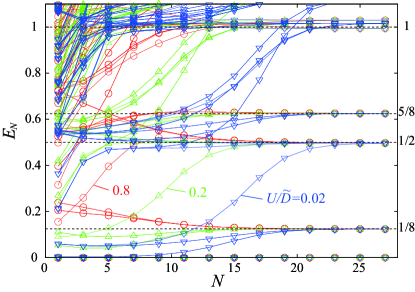
Figure 2: (Color online) NRG spectra as a function of the renormalization group step $N$ with $N$ odd for $U=0.8\tilde{D}$($\bigcirc$), $U=0.2\tilde{D}$($\bigtriangleup$) and $U=0.02\tilde{D}$($\bigtriangledown$). The spectra are uniformly scaled such that the first excited energy becomes $1/8$ for large $N$, and the identical factor is used for all three. For all three, the spectra converge on the NFL spectra $E_{\rm NFL}$ (dotted lines) for large $N$. The small deviations from $E_{\rm NFL}$ are due to truncation errors in the NRG calculations.

Table 3: Spectra $E_{N}$ at the NFL fixed point for odd $N=29$ (even $N=30$) and $U=0.02\tilde{D}$. The parity $P$ and the NRG spectra $E_{N}$ for even $N$ are shown in parentheses. $E_{N}$ is scaled such that the first excited energy with * becomes $1/8$ in order to compare $E_{N}$ with the spectra obtained by the BCFT $E_{\rm BCFT}$.

$j$	$i_{z}$	$P$	SO(5)	$E_{\rm BCFT}$	$E_{29}$ $(E_{30})$
$\frac{1}{2}$	$0$	$0(1)$	${\bf 1}$	$0$	$0\ \ (0)$
$0$	$-\frac{1}{2}$	$0(1)$	${\bf 4}$	$\frac{1}{8}$	$0.12503\ (0.125^{*})$
$0$	$-\frac{1}{2}$	$1(0)$			$0.12500\ (0.12504)$
$0$	$\frac{1}{2}$	$0(1)$			$0.12503\ (0.12500)$
$0$	$\frac{1}{2}$	$1(0)$			$0.125^{*}\ \ (0.12504)$
$\frac{1}{2}$	$-1$	$1(0)$	${\bf 5}$	$\frac{1}{2}$	$0.50155\ (0.50154)$
$\frac{1}{2}$	$0$	$0(1)$			$0.50154\ (0.50153)$
$\frac{1}{2}$	$0$	$1(0)$			$0.50124\ (0.50136)$
$\frac{1}{2}$	$0$	$1(0)$			$0.50155\ (0.50154)$
$\frac{1}{2}$	$1$	$1(0)$			$0.50155\ (0.50154)$
$1$	$-\frac{1}{2}$	$0(1)$	${\bf 4}$	$\frac{5}{8}$	$0.63098\ (0.63104)$
$1$	$-\frac{1}{2}$	$1(0)$			$0.63100\ (0.63100)$
$1$	$\frac{1}{2}$	$0(1)$			$0.63098\ (0.63104)$
$1$	$\frac{1}{2}$	$1(0)$			$0.63100\ (0.63100)$
$\frac{3}{2}$	$0$	$0(1)$	${\bf 1}$	$1$	$1.00306\ (1.00304)$
$\frac{1}{2}$	$-1$	$0(1)$	${\bf 10}$	$1$	$1.02581\ (1.02600)$
$\frac{1}{2}$	$-1$	$0(1)$			$1.02616\ (1.02620)$
$\frac{1}{2}$	$-1$	$1(0)$			$1.02615\ (1.02619)$
$\frac{1}{2}$	$0$	$0(1)$			$1.02581\ (1.02600)$
$\frac{1}{2}$	$0$	$0(1)$			$1.02616\ (1.02620)$
$\frac{1}{2}$	$0$	$1(0)$			$1.02615\ (1.02619)$
$\frac{1}{2}$	$0$	$1(0)$			$1.02580\ (1.02599)$
$\frac{1}{2}$	$1$	$0(1)$			$1.02581\ (1.02600)$
$\frac{1}{2}$	$1$	$0(1)$			$1.02616\ (1.02620)$
$\frac{1}{2}$	$1$	$1(0)$			$1.02615\ (1.02619)$
$\frac{1}{2}$	$0$	$0(1)$	${\bf 1}$	$1$	$1.03984\ (1.03992)$

The point we address in the following is how $E_{N}$ varies as a function of $N$ for the three parameters. Near the fixed point, the spectrum at the step $N$, $E_{N}$, is represented as

$$E_{N}=E_{\rm NFL}+\delta E_{N},$$ (37)

and the deviation from the fixed point value $\delta E_{N}$ is given bynrg ; zarand ; koga

$$\delta E_{N}=\sum_{r}\lambda_{r}\Lambda^{-\frac{(\Delta_{r}-1)N}{2}}.$$ (38)

Here, $r$ identifies leading irrelevant operators appearing near the fixed point. For the single channel Kondo model, $\Delta_{r}=2$.nrg In magnetic 2CKM, $\Delta_{r}=3/2$,koga which represents the “slower” renormalization than in the single channel model. Note that $\Delta_{r}$ coincides with the scaling dimension of the operator. In the following, we analyze $\delta E_{N}$ in details and examine the crossover predicted in Sec. II.2.

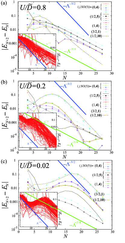
Figure 3: (Color online) $|E_{N+2}-E_{N}|$ for 15 low-energy states as a function of the renormalization group step $N$ with $N$ odd for (a) $U=0.8\tilde{D}$, (b) $U=0.2\tilde{D}$, and (c) $U=0.02\tilde{D}$. Each state is labeled by the spin $j$ and the dimension of the irreducible representation in the SO(5) group. A straight line $\sim\Lambda^{-N/2}$ is characteristic of the irrelevant operator in the SO(5) sector ${\bf L}_{-1}\cdot{\bf L}_{-1}$, while $\sim\Lambda^{-N/4}$ is characteristic of the operator in the spin sector ${\bf J}_{-1}\cdot\vec{\phi}_{s}$. Inset: the same plot for 300 low-energy states.

III.2 Crossover along the critical line

The deviation from the fixed point $\delta E_{N}$ contains information about leading irrelevant operators as shown in Eq. (38). In order to evaluate $\delta E_{N}$, we use $E_{N+2}-E_{N}$:

$$E_{N+2}-E_{N}=\sum_{r}\lambda_{r}\Lambda^{-\frac{(\Delta_{r}-1)N}{2}}(\Lambda^{1-\Delta_{r}}-1).$$ (39)

Thus, when there is a dominant leading irrelevant term with $\Delta_{r}=\Delta$, $E_{N+2}-E_{N}$ is proportional to $\Lambda^{-(\Delta-1)N/2}\sim\delta E_{N}$. Here, we use $(N+2)$- and $N$-step eigenvalues in Eq. (39), since, in NRG, there is even-odd alternation in the spectra.

Figure 3 shows $|E_{N+2}-E_{N}|$ of the low-energy states for the three parameters. Each state is labeled by the spin and the SO(5) indices: $(j,{\rm SO(5)})$. For the largest $U=0.8\tilde{D}$, it is clear that the scaling dimension $\Delta$ is $\Delta=3/2$, and thus, the NFL is described by the magnetic 2CKM as investigated in Sec. II.2. For the smallest $U=0.02\tilde{D}$, the dimension of leading irrelevant operator is $\Delta=2$, since for most of the states the $N$ dependence is $\sim\Lambda^{-N/2}$. This is consistent with our analysis in Sec. II.2.6. The $\Lambda^{-N/2}$ dependence is due to the existence of the nonmagnetic SO(5) residual interaction ${\bf L}_{-1}\cdot{\bf L}_{-1}$. In principle, there is a possibility that the term ${\bf J}_{-1}\cdot{\bf J}_{-1}$ is the origin of the $\Lambda^{-N/2}$ dependence. This possibility, however, is unlikely from a physical standpoint. It is unphysical that only the coefficient of the leading term in the spin sector is suppressed, while that of the sub-leading term in the same sector is not, as $U$ decreases.

One may find that some of the curves follow the $\Lambda^{-N/4}$ dependence for $U=0.02\tilde{D}$, but the absolute value is very small, i.e., $|\lambda_{\frac{3}{2}}|$ is very small, where we use $\Delta_{r}$ as the index $r$. Although, in principle, there exist contributions of matrix elements of the operators in the effective Hamiltonian to $|E_{N+2}-E_{N}|$, it is unlikely that the small absolute value is only due to the matrix elements, and thus, we neglect them in the following analysis. This $N$ dependence, $\Lambda^{-N/4}$, must originate in the magnetic interactions ${\bf J}_{-1}\cdot\vec{\phi}_{s}$, since in the SO(5) sector there are no such operators that generate this $N$ dependence. Note that in NRG the step $N$ is related to the energy scale as $D\Lambda^{-N/2}$, and, for example, $N=20$ corresponds to $3^{-10}D\simeq 1.69\times 10^{-5}D$. At $N=20$, the absolute value of $|\lambda_{2}|$ is more than 100 times larger than $|\lambda_{\frac{3}{2}}|$. Thus, we expect that there the spin degrees of freedom have no effect on, for example, the specific heat since $|\lambda_{2}|\gg|\lambda_{\frac{3}{2}}|$. As for the spin susceptibility, a logarithmic divergence with a very small coefficient is expected, reflecting the small $\lambda_{\frac{3}{2}}$. This is similar to the case of the flavor susceptibility in the two-channel Anderson model.2cam

As expected, the situation changes as $U$ increases. For $U=0.2\tilde{D}$, it is clear that both $\lambda_{2}$ and $\lambda_{\frac{3}{2}}$ are present with similar magnitudes. Around $N\sim 22$, the crossover from the SO(5) NFL to the NFL in 2CKM occurs. Thus, from our NRG calculations, it is clear that the profile of the leading irrelevant operators changes smoothly from the weak-coupling regime to the Kondo regime. These results confirm the results in Sec. II.2.

Finally, we discuss the impurity contributions of specific heat $C$ and the impurity entropy $S$. Figure 4 shows the temperature dependence of $(S-S_{0})/T$ and $S$ for the three parameters of $U$ with $S_{0}\simeq\ln\sqrt{2}$. Since $(S-S_{0})/T\simeq C/T$ at low temperatures, it represents $C/T$ for $T<T_{0}$. Crossover temperatures are defined as $T_{0}\equiv\tilde{D}\Lambda^{-N_{0}/2}$. For large $U/{\tilde{D}}=0.8$, $C/T$ at low temperatures diverges logarithmically and this is consistent with the conventional magnetic 2CKM. As expected from the results of the scaling dimension of leading irrelevant operators, the temperature dependence of $C/T$ changes with decreasing $U$. One can clearly see that it is constant at low temperatures for $U/\tilde{D}=0.02$ and $0.2$. For $T<T_{0}$, the temperature dependence of entropy for $U/\tilde{D}=0.02$ and $0.2$ is well described by a single-scale function of $(T/T_{0})\sim(T/T_{L})$, while that for $U/\tilde{D}=0.8$ has a different functional form, since $T_{0}\sim T_{s}$ for $U/\tilde{D}=0.8$. For $U/\tilde{D}=0.2$, the temperature dependence changes from $\sim$ const. to $-\ln T$, and the crossover temperature has been defined as $T^{*}$ in Eq. (34). This is the crossover from the SO(5)-operator dominant regime to the spin-operator dominant regime. Below $T\sim T^{*}$, the temperature dependence of $S$ is not described by the single-scale function of $(T/T_{L})$, although the deviation in $S$ is very small $\sim-T\ln T$. Note that the impurity entropy $S$ is $S\simeq\ln\sqrt{2}$ for the temperature where $C/T=$ const. appears. These results confirm our BCFT predictions and the importance of nonmagnetic SO(5) degrees of freedom for small $U$.

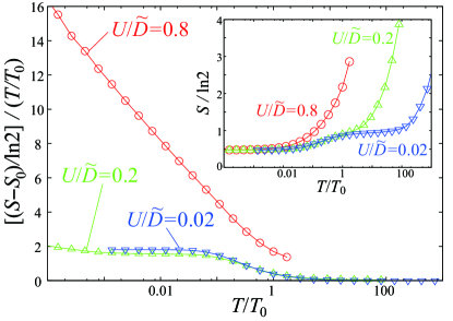
Figure 4: (Color online) Temperature dependence of $(S-S_{0})/T$ for the three values of $U$. Temperature $T$ is scaled by $T_{0}$; $T_{0}/{\tilde{D}}=0.192$ for $U/{\tilde{D}}=0.8$, $T_{0}/{\tilde{D}}=0.00713$ for $U/{\tilde{D}}=0.2$, and $T_{0}/{\tilde{D}}=0.000264$ for $U/{\tilde{D}}=0.02$. Inset: Temperature dependence of $S$.

IV Discussion and Summary

In this paper, we have analyzed low-energy critical theory in a two-channel Anderson model with phonon-assisted hybridization on the basis of BCFT and NRG. One important finding is that nonmagnetic SO(5) degrees of freedom are constructed in the ${\bf I}\otimes\vec{\tau}$ sector, which are “hidden” in the 2CKM due to the Hilbert space restriction, and also the conduction electron part is rewritten by the SO(5) currents. These nonmagnetic degrees of freedom are important for small $U$. We have demonstrated that SO(5)-${\bf 4}$ fusion gives exactly the same NFL spectra as those in the magnetic 2CKM. The difference between the spin-1/2 and the SO(5)-${\bf 4}$ fusions have been discussed and we interpret the fusion as simply equivalent ones, noticing that the spin-1/2 fusion and the $\pi/2$ phase shift in the Anderson model are equivalent. A full understanding of the exact fusion process will require a more sophisticated analysis.

In the form of residual effective interaction (32), the crossover between small and large $U$ can be described by changes in the coefficients $\lambda_{s}$ and $\lambda_{L}$ in Eq. (32). Note that the residual interactions in the SO(5) sector never appear if we map the model to the magnetic 2CKM, since there is no $\lambda_{L}{\bf L}(0)\cdot{\bf L}(0)$ term in the perturbation expansion in the spin sector. Using physical intuition, we predict that the SO(5) sector is more important than the spin sector for small $U$, leading to linear specific heat at low temperatures. This has been checked by the NRG calculations; the scaling dimension of leading irrelevant operators varies from $\Delta=3/2$ to $\Delta=2$ as $U$ decreases, and the impurity contribution of specific heat is proportional to temperature for small $U$.

The difference between the present NFL for small $U$ and the NFL in the two-level systems should be noted, although they both have a nonmagnetic origin. It is well known that the NFL spectra in the two-level Kondo model is derived via flavor-1/2 fusion.Cox The spectra is the same as those in the magnetic 2CKM when the spin and the flavor sector are interchanged, while the present NFL spectra are exactly the same as those in the magnetic 2CKM. The scaling dimension of the leading irrelevant operator in the two-level Kondo model is 3/2, which leads to a logarithmic diverging specific heat coefficient. Thus, nonmagnetic Kondo phenomena in the two models should be distinguished and the microscopic mechanism for the NFL in each of the models is quite different, i.e., flavor SU(2) and nonmagnetic SO(5) exchange interactions.

Our BCFT analysis can also be applicable to the anharmonic model investigated in Ref. 24, since even in the anharmonic phonon model, parity $P$ is a good quantum number and the phonon states in the effective theory would be described by $\vec{\tau}$ as in a similar manner to that of the present analysis. With regard to the generalization of this model to the more realistic one, it is interesting to take into account optical modes that couple with localized electrons. This electron-phonon coupling reduces the bare Coulomb repulsion. When it is sufficiently large, the effective Coulomb interaction becomes attractive, and thus, it is possible to realize another NFL fixed point in which the spin and charge sector are interchanged from the present NFL for $U>0$. With regard to a lattice generalization of the present model, it is also interesting to examine whether some composite pairing operators listed in Table 1 condensate into exotic superconducting states.

In summary, we have investigated the microscopic origin of the line of non-Fermi liquid fixed points found previously by numerical simulations.Daggoto ; Yashiki1 ; Yashiki2 We have succeeded in constructing nonmagnetic SO(5) degrees of freedom, and, on the basis of boundary conformal field theory, we have pointed out that, for the weak electron-electron correlation regime, the non-Fermi liquid can be interpreted as an SO(5) non-Fermi liquid, which crosses overs to a non-Fermi liquid in the Kondo regime. We have also analyzed the difference in the leading irrelevant operators as $U$ varies, and indeed we have confirmed it by numerical simulations. In particular, the impurity contributions to the specific heat are proportional to temperature $T$ for small $U$, while they are proportional to $-T\ln T$ for large $U$. The present results demonstrate that it is important to take into account not only single degrees of freedom, e.g., only a phonon, but also complex degrees of freedom formed both by electrons and phonons in the Kondo problems in electron-phonon coupled systems.

Appendix A Matrix representations of SO(5) Generators and Vectors

In this Appendix, we summarize the definitions of SO(5) matrices. We follow the convention used by Wu, et al.Wu

A.1 Generators: 10 representation

The SO(5) generators $\mathcal{L}^{ab}$ define all the SO(5) rotation and are given by ${\mathcal{L}}^{ab}\equiv\Gamma^{ab}/2$ with

$$\Gamma^{12} = -\begin{pmatrix}0&0&0&1\\ 0&0&1&0\\ 0&1&0&0\\ 1&0&0&0\end{pmatrix},\ \ \Gamma^{13}=\begin{pmatrix}0&0&0&i\\ 0&0&-i&0\\ 0&i&0&0\\ -i&0&0&0\end{pmatrix},$$

$$\Gamma^{14} = \begin{pmatrix}0&0&-1&0\\ 0&0&0&1\\ -1&0&0&0\\ 0&1&0&0\end{pmatrix},\ \ \Gamma^{15}=\begin{pmatrix}-1&0&0&0\\ 0&-1&0&0\\ 0&0&1&0\\ 0&0&0&1\end{pmatrix},$$

$$\Gamma^{23} = \begin{pmatrix}1&0&0&0\\ 0&-1&0&0\\ 0&0&1&0\\ 0&0&0&-1\end{pmatrix},\ \ \Gamma^{24}=\begin{pmatrix}0&i&0&0\\ -i&0&0&0\\ 0&0&0&i\\ 0&0&-i&0\end{pmatrix},$$

$$\Gamma^{25} = \begin{pmatrix}0&0&0&i\\ 0&0&i&0\\ 0&-i&0&0\\ -i&0&0&0\end{pmatrix},\ \ \Gamma^{34}=\begin{pmatrix}0&1&0&0\\ 1&0&0&0\\ 0&0&0&1\\ 0&0&1&0\end{pmatrix},$$

$$\Gamma^{35} = \begin{pmatrix}0&0&0&1\\ 0&0&-1&0\\ 0&-1&0&0\\ 1&0&0&0\end{pmatrix},\ \ \Gamma^{45}=\begin{pmatrix}0&0&i&0\\ 0&0&0&-i\\ -i&0&0&0\\ 0&i&0&0\end{pmatrix}.$$

$\mathcal{L}^{ab}$’s are ten-dimensional adjoint representation ${\bf 10}$ and satisfy the following SO(5) commutation relations:

$$[\mathcal{L}^{ab},\mathcal{L}^{cd}] = -i(\delta_{bc}\mathcal{L}^{ad}-\delta_{ac}\mathcal{L}^{bd}-\delta_{bd}\mathcal{L}^{ac}+\delta_{ad}\mathcal{L}^{bc}),\ \ \ \ \ \ \$$ (41)

$$\equiv if^{ab,cd,ef}{\mathcal{L}}^{ef},$$ (42)

where the repeated indices are assumed to be summed over and $1\leq a<b\leq 5$, $1\leq c<d\leq 5$, and $1\leq e<f\leq 5$. $\mathcal{L}^{ab}$ with $a>b$ should be regarded as $\mathcal{L}^{ab}=-{\mathcal{L}}^{ba}$ on the right-hand side of Eq. (41).

A.2 Vectors:  5 representations

The ${\bf 5}$ representation is an SO(5) vector and is represented by the following five matrices:

$$\Gamma^{1} = \begin{pmatrix}0&0&i&0\\ 0&0&0&i\\ -i&0&0&0\\ 0&-i&0&0\end{pmatrix},\ \ \Gamma^{2}=\begin{pmatrix}0&1&0&0\\ 1&0&0&0\\ 0&0&0&-1\\ 0&0&-1&0\end{pmatrix},$$

$$\Gamma^{3} = \begin{pmatrix}0&-i&0&0\\ i&0&0&0\\ 0&0&0&i\\ 0&0&-i&0\end{pmatrix},\ \ \Gamma^{4}=\begin{pmatrix}1&0&0&0\\ 0&-1&0&0\\ 0&0&-1&0\\ 0&0&0&1\end{pmatrix},$$

$$\Gamma^{5} = -\begin{pmatrix}0&0&1&0\\ 0&0&0&1\\ 1&0&0&0\\ 0&1&0&0\end{pmatrix}.$$ (43)

In terms of $\Gamma^{a}$’s, $\Gamma^{ab}$’s are represented as

$$\Gamma^{ab}=\frac{1}{2i}[\Gamma^{a},\Gamma^{b}].$$ (44)

The commutation relations between $\Gamma^{a}$ and $\Gamma^{bc}$ are given by

$$[\Gamma^{a},{\Gamma}^{bc}]=-2i\Big{(}{\rm sgn}(c-a)\delta_{ab}\Gamma^{c}+{\rm sgn}(b-a)\delta_{ac}\Gamma^{b}\Big{)}.\ \$$ (45)

Appendix B Axial Charge

In this Appendix, we summarize various spherical tensors with respect to the axial charge. They appear as a part of the SO(5) degrees of freedom in the main text.

B.1 Spherical tensors of axial charge symmetry

Spherical tensor operators $T_{m}^{(l)}$ in the axial charge sector are defined by

$$[{I_{\rm tot}}_{z},T_{m}^{(l)}] = mT_{m}^{(l)},$$ (46)

$$[{I_{\rm tot}}_{\pm},T_{m}^{(l)}] = \sqrt{(l\mp m)(l\pm m+1)}T_{m\pm 1}^{(l)}.$$ (47)

Here, ${\bf I}_{\rm tot}$ is defined by Eqs. (3) and (4) and $l$ is an integer and is called the rank of operator $T^{(l)}_{m}$ and $|m|\leq l$. Operators with $l=0$ are scalar, i.e., invariant under the charge SU(2) operations, while operators with $l\geq 1$ transform as rank-$l$ tensors. In particular, operators with $l=1$ transform as vectors. A trivial example is the axial charge of conduction electrons ${\bf I}(x)$,

$$I_{z}(x) = \frac{1}{2}\sum_{\sigma}\Big{[}s^{\dagger}_{\sigma}(x)s_{\sigma}(x)+p^{\dagger}_{\sigma}(x)p_{\sigma}(x)-1\Big{]},$$ (48)

$$I_{+}(x) = s_{\uparrow}^{\dagger}(x)s_{\downarrow}^{\dagger}(x)+p_{\uparrow}^{\dagger}(x)p_{\downarrow}^{\dagger}(x)=[I_{-}(x)]^{\dagger}.$$ (49)

${\bf I}(x)$ denotes the contributions of the conduction electrons to ${\bf I}_{\rm tot}$axialchargeNOTE and the rank-1 tensor with $[T^{(1)}_{-1},T^{(1)}_{0},T^{(1)}_{1}]$$=$$[I_{-}(x)/\sqrt{2},I_{z}(x),-I_{+}(x)/\sqrt{2}]$. Thus, the quantum number of ${\bf I}(x)$ is $(j_{j_{z}},i,P)=(0_{0},1,0)$, where, $j(i)$ is the eigenvalue of spin (axial charge) with the z-component $j_{z}$ and $P$ is the parity. Here, the quantum numbers in the spin sector can be determined in the same way as in the axial charge sector. The quantum numbers of the $f$-electron axial charge ${\bf I}$ are the same as those of ${\bf I}(x)$. In the following, we will list various spherical tensors that appear in the SO(5) degrees of freedom analyzed in the main text.

B.2 Longitudinal-flavor axial charge

We define longitudinal-flavor axial charge ${\bf I}^{\prime}(x)$, which is related to the SO(5) generator $L^{12}(x)$, $L^{23}(x)$ and $L^{25}(x)$, and appears in Eq. (LABEL:II) as

$$I^{\prime}_{z}(x) = \frac{1}{2}\sum_{\sigma}\Big{[}s^{\dagger}_{\sigma}(x)s_{\sigma}(x)-p^{\dagger}_{\sigma}(x)p_{\sigma}(x)\Big{]},$$ (50)

$$I^{\prime}_{+}(x) = s_{\uparrow}^{\dagger}(x)s_{\downarrow}^{\dagger}(x)-p_{\uparrow}^{\dagger}(x)p_{\downarrow}^{\dagger}(x)=[I^{\prime}_{-}(x)]^{\dagger}.$$ (51)

The parity of these operators is even, since $p_{\sigma}$ appears as quadratic forms in Eqs. (50) and (51). In terms of the spherical tensors, ${\bf I}^{\prime}(x)$ is the rank 1 tensor with $[T^{(1)}_{-1},T^{(1)}_{0},T^{(1)}_{1}]$$=$$[I^{\prime}_{-}(x)/\sqrt{2},I^{\prime}_{z}(x),-I^{\prime}_{+}(x)/\sqrt{2}]$. Thus, the quantum number of ${\bf I}^{\prime}(x)$ is $(j_{j_{z}},i,P)=(0_{0},1,0)$.

B.3 Transverse-flavor axial charge

We define transverse-flavor axial charge ${\bf I}^{\prime\prime}(x)$, which is related to $L^{14}(x)$, $L^{34}(x)$ and $L^{45}(x)$, and appears in Eq. (LABEL:II) as

$$I^{\prime\prime}_{z}(x) = \frac{1}{2}\sum_{\sigma}\Big{[}p^{\dagger}_{\sigma}(x)s_{\sigma}(x)+s^{\dagger}_{\sigma}(x)p_{\sigma}(x)\Big{]},$$ (52)

$$I^{\prime\prime}_{+}(x) = s_{\uparrow}^{\dagger}(x)p_{\downarrow}^{\dagger}(x)+p_{\uparrow}^{\dagger}(x)s_{\downarrow}^{\dagger}(x)=[I^{\prime\prime}_{-}(x)]^{\dagger}.$$ (53)

The parity of these operators is odd, since ${\bf I}^{\prime\prime}(x)$ includes one $p_{\sigma}$ in each term. In terms of the spherical tensors, ${\bf I}^{\prime\prime}(x)$ is the rank 1 tensor and $[T^{(1)}_{-1},T^{(1)}_{0},T^{(1)}_{1}]$$=$$[I^{\prime\prime}_{-}(x)/\sqrt{2},I^{\prime\prime}_{z}(x),-I^{\prime\prime}_{+}(x)/\sqrt{2}]$. Thus, the quantum number of ${\bf I}^{\prime\prime}(x)$ is $(j_{j_{z}},i,P)=(0_{0},1,1)$.

B.4 Flavor singlet

We define a flavor singlet operator ${\mathcal{D}}(x)=L^{24}(x)$, which appears in Eq. (LABEL:II) as

$${\mathcal{D}}(x) = -\frac{i}{2}\sum_{\sigma}\Big{[}s^{\dagger}_{\sigma}(x)p_{\sigma}(x)-p^{\dagger}_{\sigma}(x)s_{\sigma}(x)\Big{]}.$$ (54)

The parity of this operator is odd, as is evident from the fact that $\mathcal{D}(x)$ includes one $p_{\sigma}$ in each term. Since $[{I_{\rm tot}}_{\pm},{\mathcal{D}}(x)]=0$ and $[{I_{\rm tot}}_{z},{\mathcal{D}}(x)]=0$, $\mathcal{D}(x)$ is a scalar operator and the quantum number of $\mathcal{D}(x)$ is $(j_{j_{z}},i,P)=(0_{0},0,1)$.

B.5 Longitudinal spin-flavor singlet

We define a longitudinal spin-flavor singlet operator ${\mathcal{D}}^{\prime}(x)=n^{4}(x)$, i.e., the fourth component of the SO(5) vector ${\bf n}(x)$ in Table 1 as

$${\mathcal{D}}^{\prime}(x) = \frac{1}{2}\sum_{\sigma}\sigma\Big{[}s^{\dagger}_{\sigma}(x)s_{\sigma}(x)-p^{\dagger}_{\sigma}(x)p_{\sigma}(x)\Big{]}.$$ (55)

The parity of this operator is even, as is evident from the fact that $\mathcal{D}^{\prime}(x)$ includes zero or two $p_{\sigma}$’s in each term. Since $[{I_{\rm tot}}_{\pm},{\mathcal{D}}^{\prime}(x)]=0$ and $[{I_{\rm tot}}_{z},{\mathcal{D}}^{\prime}(x)]=0$, $\mathcal{D}^{\prime}(x)$ is a scalar operator and the quantum number of $\mathcal{D}^{\prime}(x)$ is $(j_{j_{z}},i,P)=(1_{0},0,0)$.

B.6 Transverse spin-flavor singlet

We define a transverse spin-flavor singlet operator ${\mathcal{D}}^{\prime\prime}(x)=n^{2}(x)$ in Table 1 as

$${\mathcal{D}}^{\prime\prime}(x) = \frac{1}{2}\sum_{\sigma}\sigma\Big{[}p^{\dagger}_{\sigma}(x)s_{\sigma}(x)+s^{\dagger}_{\sigma}(x)p_{\sigma}(x)\Big{]}.$$ (56)

The parity of this operator is odd, since $\mathcal{D}^{\prime\prime}(x)$ includes one $p_{\sigma}$ in each term. Since $[{I_{\rm tot}}_{\pm},{\mathcal{D}}^{\prime\prime}(x)]=0$ and $[{I_{\rm tot}}_{z},{\mathcal{D}}^{\prime\prime}(x)]=0$, $\mathcal{D}^{\prime\prime}(x)$ is a scalar operator and the quantum number of $\mathcal{D}^{\prime\prime}(x)$ is $(j_{j_{z}},i,P)=(1_{0},0,1)$.

B.7 Transverse-spin-flavor axial charge

We define transverse-spin-flavor axial charge ${\bf I}^{\prime\prime\prime}(x)$, which is related to $n^{1}(x)$, $n^{3}(x)$ and $n^{5}(x)$ in Table 1 as

$$I^{\prime\prime\prime}_{z}(x) = \frac{i}{2}\sum_{\sigma}\sigma\Big{[}p^{\dagger}_{\sigma}(x)s_{\sigma}(x)-s^{\dagger}_{\sigma}(x)p_{\sigma}(x)\Big{]},$$ (57)

$$I^{\prime\prime\prime}_{+}(x) = -i\Big{[}s_{\uparrow}^{\dagger}(x)p_{\downarrow}^{\dagger}(x)+s_{\downarrow}^{\dagger}(x)p_{\uparrow}^{\dagger}(x)\Big{]}=[I^{\prime\prime\prime}_{-}(x)]^{\dagger}.\ \ \ \ \ \ \ \$$ (58)

The parity of these operators is odd, since ${\bf I}^{\prime\prime\prime}(x)$ includes one $p_{\sigma}$ in each term. In terms of the spherical tensors, ${\bf I}^{\prime\prime\prime}(x)$ is the rank 1 tensor with $[T^{(1)}_{-1},T^{(1)}_{0},T^{(1)}_{1}]$$=$$[I^{\prime\prime\prime}_{-}(x)/\sqrt{2},I^{\prime\prime\prime}_{z}(x),-I^{\prime\prime\prime}_{+}(x)/\sqrt{2}]$. Thus, the quantum number of ${\bf I}^{\prime\prime\prime}(x)$ is $(j_{j_{z}},i,P)=(1_{0},1,1)$.

Appendix C Primary states of SO(5)₂ Kac-Moody algebra

In this Appendix, we briefly show that the primary states for $k=2$ SO(5) Kac-Moody algebra are ${\bf 1}$, ${\bf 4}$, and ${\bf 5}$ representations.

Since the rank of SO(5) group is 2 and thus the Cartan subalgebra consists of $H_{1}\equiv L_{0}^{15}$ and $H_{2}\equiv L_{0}^{23}$, we can label primary states by their eigenvalues, $h_{1}$ and $h_{2}$, and denote them as $|h_{1},h_{2}\rangle$ with $h_{1}$ and $h_{2}$ being integers or half-integers. Since $|h_{1},h_{2}\rangle$ is primary, $L_{n}^{ab}|h_{1},h_{2}\rangle=0$ for $n>0$. Ladder operators are defined as

$$J_{-}^{(1)} \equiv L_{0}^{34}+iL_{0}^{24}\equiv[J_{+}^{(1)}]^{\dagger},$$ (59)

$$J_{-}^{(2)} \equiv \frac{1}{2}\Big{[}L_{0}^{35}-L_{0}^{12}-iL_{0}^{13}-iL_{0}^{25}\Big{]}\equiv[J^{(2)}_{+}]^{\dagger},$$ (60)

and they satisfy

$$[H_{1},J_{-}^{(1)}]=0,\ \ \ \ \ \ \ \ \ \ [H_{2},J_{-}^{(1)}]=-J_{-}^{(1)},$$ (61)

$$[H_{1},J_{-}^{(2)}]=-J_{-}^{(2)},\ \ \ \ [H_{2},J_{-}^{(2)}]=J_{-}^{(2)}.$$ (62)

The commutation relations Eqs. (61) and (62) indicate $J_{-}^{(1)}|h_{1},h_{2}\rangle\propto|h_{1},h_{2}-1\rangle$ and $J_{-}^{(2)}|h_{1},h_{2}\rangle\propto$$|h_{1}-1,h_{2}+1\rangle$.

Similarly, we can define another set of ladder operators as

$$\tilde{J}_{-}^{(1)} \equiv L_{+1}^{34}+iL_{+1}^{24}\equiv[\tilde{J}_{+}^{(1)}]^{\dagger},$$ (63)

$$\tilde{J}_{-}^{(2)} \equiv \frac{1}{2}\Big{[}L_{+1}^{35}-L_{+1}^{12}-iL_{+1}^{13}-iL_{+1}^{25}\Big{]}\equiv[\tilde{J}^{(2)}_{+}]^{\dagger},$$ (64)

where $L_{+1}^{ab}=[L_{-1}^{ab}]^{\dagger}$. Straightforward calculations show that they satisfy

$$[H_{1},\tilde{J}_{-}^{(1)}]=0,\ \ \ \ \ \ \ \ \ \ [H_{2},\tilde{J}_{-}^{(1)}]=-\tilde{J}_{-}^{(1)},$$ (65)

$$[H_{1},\tilde{J}_{-}^{(2)}]=-\tilde{J}_{-}^{(2)},\ \ \ \ [H_{2},\tilde{J}_{-}^{(2)}]=\tilde{J}_{-}^{(2)},$$ (66)

and also satisfy

$$[\tilde{J}_{+}^{(1)},\tilde{J}_{-}^{(1)}] = 2H_{2}-k,$$ (67)

and

$$[\tilde{J}_{+}^{(2)},\tilde{J}_{-}^{(2)}] = H_{1}-H_{2}-k/2.$$ (68)

Now, let us consider the norm of descendant states. Since the norm is positive, we obtain

$$|\tilde{J}_{+}^{(1)}|h_{1},h_{2}\rangle|^{2} = \langle h_{1},h_{2}|\tilde{J}_{-}^{(1)}\tilde{J}_{+}^{(1)}|h_{1},h_{2}\rangle,$$ (69)

$$= \langle h_{1},h_{2}|[\tilde{J}_{-}^{(1)},\tilde{J}_{+}^{(1)}]|h_{1},h_{2}\rangle,$$

$$= -2h_{2}+k\geq 0,$$

where at the second line we have used $L_{+1}^{ab}|h_{1},h_{2}\rangle=0$ and at the third line, Eq. (67) and $\langle h_{1},h_{2}|h_{1},h_{2}\rangle=1$ have been used. Similar calculations for $\tilde{J}_{+}^{(2)}|h_{1},h_{2}\rangle$ lead to

$$h_{2}-h_{1}+k/2\geq 0.$$ (70)

It is clear that irreducible representations with the large dimension cannot satisfy Eqs. (69) and (70), since, in general, such irreducible representations have large $|h_{1}|$ and $|h_{2}|$. Indeed, Eqs. (69) and (70) indicate that there are three irreducible representations, and they are the identity ${\bf 1}$, the spinor ${\bf 4}$, and the vector ${\bf 5}$. Thus, primary states in the SO(5)₂ sector belong to ${\bf 1}$, ${\bf 4}$, or ${\bf 5}$ representations.

References

- (1) J. Kondo, Prog. Theor. Phys. 32, 37 (1964).
- (2) C. C. Yu and P. W. Anderson, Phys. Rev. B 29, 6165 (1984).
- (3) T. Matsuura and K. Miyake, J. Phys. Soc. Jpn. 55, 610 (1986).
- (4) K. Vladár and A. Zawadowski, Phys. Rev. B 28, 1564 (1983).
- (5) K. Vladár and A. Zawadowski, Phys. Rev. B 28, 1582 (1983).
- (6) K. Vladár and A. Zawadowski, Phys. Rev. B 28, 1596 (1983).
- (7) A. L. Moustakas and D. S. Fisher, Phys. Rev. B 51, 6908 (1995).
- (8) A. L. Moustakas and D. S. Fisher, Phys. Rev. B 55, 6832 (1997).
- (9) H. Kusunose and K. Miyake, J. Phys. Soc. Jpn. 65, 3032 (1996).
- (10) S. Yotsuhashi, M. Kojima, H. Kusunose, and K. Miyake, J. Phys. Soc. Jpn. 74, 49 (2005).
- (11) K. Hattori, Y. Hirayama, and K. Miyake, J. Phys. Soc. Jpn. 74, 3306 (2005).
- (12) T. Hotta, J. Phys. Soc. Jpn. 76, 023705 (2007).
- (13) T. Hotta, J. Phys. Soc. Jpn. 77, 103711 (2008).
- (14) T. Hotta, J. Phys. Soc. Jpn. 78, 073707 (2009).
- (15) S. Sanada, Y. Aoki, H. Aoki, A. Tsuchiya, D. Kikuchi, H. Sugawara, and H. Sato, J. Phys. Soc. Jpn. 74, 246 (2005).
- (16) B. C. Sales, B. C. Chakoumakos, R. Jin, J. R. Thompson, and D. Mandrus, Phys. Rev. B 63, 245113 (2001).
- (17) Z. Hiroi, J. Yamaura, and K. Hattori, J. Phys. Soc. Jpn. 81, 011012 (2012).
- (18) P. Nozières and A. Blandin, J. Phys. (Paris) 41, 193 (1980)
- (19) L. G. G. V. Dias da Silva and E. Dagotto, Phys. Rev. B 79, 155302 (2009).
- (20) S. Yashiki, S. Kirino, and K. Ueda, J. Phys. Soc. Jpn. 79, 093707 (2010).
- (21) S. Yashiki, S. Kirino, K. Hattori, and K. Ueda, J. Phys. Soc. Jpn. 80, 064701 (2011).
- (22) T. Hotta and K. Ueda, Phys. Rev. Lett. 108, 247214 (2012).
- (23) K. G. Wilson, Rev. Mod. Phys. 47, 773 (1975).
- (24) S. Yashiki and K. Ueda, J. Phys. Soc. Jpn. 80, 084717 (2011).
- (25) I. Affleck and A. W. W. Ludwig, Phys. Rev. Lett. 67, 161 (1991).
- (26) D. L. Cox and A. Zawadowski, Adv. in Phys. 47, 599 (1998).
- (27) In order to make and terms in Eq. (1) invariant, components of the conduction electron local axial charge should be defined with an opposite sign to that of . Similarly, the sign of should be opposite to that for the neighboring sites in the effective one-dimensional lattice and also in NRG calculations. In the conformal field theoretical approach, the definition of is (49) without the sign factor as discussed by Kim et al.: T. S. Kim, L. N. Oliveira, and D. L. Cox, Phys. Rev. B, 55, 12460 (1997).
- (28) For , similar phase diagram is expected. For large , two-channel charge Kondo critical point is realized and the physics for small can be discussed in the same way as for small in the main text with exchanging the spin and axial charge sector.
- (29) I. Affleck, Nucl. Phys. B336, 517 (1990).
- (30) I. Affleck and A. W. W. Ludwig, Nucl. Phys. B352, 849 (1991).
- (31) I. Affleck and A. W. W. Ludwig, Nucl. Phys. B360, 641 (1991).
- (32) I. Affleck, A. W. W. Ludwig, H.-B. Pang, and D. L. Cox, Phys. Rev. B 45, 7918 (1992).
- (33) C. Wu, J.-p. Hu, and S.-c. Zhang, Phys. Rev. Lett. 91, 186402 (2003).
- (34) K. Hattori, J. Phys. Soc. Jpn. 74, 3135 (2005).
- (35) C. Itzykson and J.-M. Drouffe, “Statistical Field Theory” (Cambridge University Press, Cambridge, 1989) Vol. 2.
- (36) I. G. Lang and Yu. A. Firsov, Zh. Eksp. Theor. Fiz. 43, 1843 (1962), [Sov. Phys. JETP 16, 1301 (1963)].
- (37) A. W. W. Ludwig, Int. J. Mod. Phys. B 8, 347 (1994).
- (38) H. Johannesson, N. Andrei, and C. J. Bolech, Phys. Rev. B 68, 075112 (2003).
- (39) J. von Delft, G. Zaránd, and M. Fabrizio, Phys. Rev. Lett. 81, 196 (1998).
- (40) M. Koga, G. Zaránd, and D. L. Cox, Phys. Rev. Lett. 83, 2421 (1999).
- (41) K. Hattori, unpublished.
- (42) This fixed point can be characterized by three different phenomenological pictures. One is to regard it as that with non-interacting -electrons plus decoupled . The second is to regard it as a system with antiferromagnetic strong coupling spin exchange interactions between the f- and p-electrons and also decoupled . Thirdly, in our language in Sec. II.2, it is characterized by strong coupling antiferro axial charge exchange interactions between the f- and p-electrons and again with decoupled .