Efficient graphene-based photodetector with two cavities

Abstract

We present an efficient graphene-based photodetector with two Fabri-Pérot cavities. It is shown that the absorption can reach almost 100% around a given frequency, which is determined by the two-cavity lengths. It is also shown that hysteresis in the absorbance is possible, with the transmittance amplitude of the mirrors working as an external driving field. The role of non-linear contributions to the optical susceptibility of graphene is discussed.

I Introduction

Exploring the optical properties of graphenermp ; nair ; rmpperes for photodetection is one of the most promising applications of graphene.Avouris Graphene has no gap and its conductivity is essentially independent of frequencynmrPRB06 ; abergel ; gusyninIJMPB ; falkov1 ; falkov2 for photon energies up to 2 eV. These properties, combined with the intrinsic chemical and mechanical stability of graphene, pave the way for broad band optoelectronics.

Depending on the authors, graphene is characterized as presenting remarkable high absorptionAbajo or weak absorption.Novoselov Indisputable however is the fact that pristine graphene absorbs about 2.3% of the light impinging on it. A considerable frequency dependence of the absorption appears as the photon energy approaches $\sim 4.7$ eV, due to the combined effects of the Van Hove singularity in graphene’s electronic $\pi-$spectrum and excitonic many-body effects.LiLouie The value of 2.3% can also be interpreted as the probability for photon absorption in a single passing through the material.

To enhance the absorption of graphene several mechanisms have been proposed, ranging from hybrid materials, containing carbon, boron, and nitrogen,Novoselov ; NewDirections nano-patterning of a graphene sheetFullAbajo , to strain engineering,Novoselov ; NewDirections and plasmonics.Ozbay ; EPLPeres In the latter case, micro-sized ribbons patterned in a single graphene sheet,Zettl and metallic arrays on top of graphene,Geim lead to an enhancement of the near field, thus increasing light absorption and producing larger photo-currents compared to the case of pristine graphene. Current plasmonics-based approaches are limited to specific spectral bands. In what concerns hybrid materials for photonic applications, there is still a long way to go before these become possible.Novoselov ; NewDirections

Photodetection, depending on the type of application, may require efficient absorption of light in a narrow spectral band. Then, it is conceivable to explore Fabry-Pérot interference for producing an efficient photodetector tailored for a specific application. The concept is simple: in a Fabry-Pérot interferometer a photon may be trapped inside the cavity for a long time, undergoing many round trips before leaving it; indeed, if a material able to absorb photons is introduced inside the optical cavity, without significantly changing the cavity’s finesse, as is the case of graphene, most of the photons of the right frequency entering the optical cavity will be absorbed.

For a combined cavity-graphene system, it is important to quantity the magnitude of non-linear optical effects, ensuring whether linear response theory can be used for describing the absorption process inside the cavity. Thus, in the present work, we discuss the non-linear optical susceptibility of graphene first, presenting later the single and double cavity photodetectors.

This article is organized as follows: in Sec. II we introduce Bloch’s equations for graphene and compute both the linear and non-linear optical susceptibility. As aforementioned, the calculation of the non-linear part is essential for a critical analysis of the optical response of graphene. In Sec. III we give the power series solution of Bloch’s equation and discuss the validity of perturbation theory. In Sec. IV we introduce the mathematical description of a graphene-based photodetector. Having shown that non-linear contributions to the optical susceptibility are relevant only at very high field intensities, we employ linear response theory to describe the graphene-based photodetector with two coupled optical cavities.

II Derivation of Bloch equations of motion

The calculation of the optical properties of a given material can be obtained from the solution of Bloch’s equations.Haug ; Malic ; Peres_Excitonic ; EOM Below, we derive Bloch’s differential equations for graphene and give its solution for an incoming electromagnetic plane wave impinging on the material.

The Hamiltonian of the electrons in graphene, in the presence of an electromagnetic field, reads (spin index implicit):

$$H = \sum_{\bm{k}}E_{c}(\bm{k})a_{c,\bm{k}}^{{\dagger}}a_{c,\bm{k}}+E_{v}(\bm{k})a_{v,\bm{k}}^{{\dagger}}a_{v,\bm{k}}$$ (1)

$$+ v_{F}eA(t)\sum_{\bm{k}}(d_{cv,\bm{k}}^{x}a_{c,\bm{k}}^{{\dagger}}a_{v,\bm{k}}+d_{vc,\bm{k}}^{x}a_{v,\bm{k}}^{{\dagger}}a_{c,\bm{k}})\,,$$

where $E_{c/v}(\bm{k})=\pm v_{F}\hbar k$, $v_{F}=3ta_{0}/\hbar$ is the Fermi velocity ($t\simeq 2.7$ eV and $a_{0}=1.4$ Å  are the hoping integral and the carbon-carbon distance, respectively), $a_{c/v,\bm{k}}^{{\dagger}}$ is the creation operator of an electron with wave number $\bm{k}$ in the conduction/valence band,

$$d_{vc,k}^{x}=-i\sin\theta$$ (2)

is the matrix element of the dipole operator ($d_{cv,k}^{x}=i\sin\theta$), $A(t)=A_{0}\sin(\omega t)$ is the vector potential for a linearly polarized electromagnetic plane wave, $e>0$ is the elementary charge, $\omega$ is the frequency of light, and

$$\theta=\arctan\frac{k_{y}}{k_{x}}\,.$$ (3)

Since we have $E(t)=-\frac{\partial A(t)}{\partial t}=-\omega A_{0}\cos(\omega t)\,,$ we can write $A(t)$ as

$$A(t)=i\frac{E_{0}}{2\omega}e^{-i\omega t}+\frac{E_{0}}{2i\omega}e^{i\omega t}\,,$$ (4)

where $E_{0}$ is the intensity of the electric field.

At the heart of the present approach is Heisenberg’s equation of motion for the polarization operator $\hat{P}_{vc,\bm{k}}\equiv a_{v,\bm{k}}^{{\dagger}}a_{c,\bm{k}}$, namely,

$$-i\hbar\frac{d\hat{P}_{vc,\bm{k}}}{dt}=[H,\hat{P}_{vc,\bm{k}}]\,.$$ (5)

The explicit form of the equation of motion is

$$-i\hbar\frac{d\hat{P}_{vc,\bm{k}}}{dt} - i\hbar\gamma_{2,\bm{k}}\hat{P}_{vc,\bm{k}}=-[E_{c}(\bm{k})-E_{v}(\bm{k})]\hat{P}_{vc,\bm{k}}$$ (6)

$$+ v_{F}eA(t)(a_{c,\bm{k}}^{{\dagger}}a_{c,\bm{k}}-a_{v,\bm{k}}^{{\dagger}}a_{v,\bm{k}})d_{cv,\bm{k}}^{x}\,.$$

In the above, $\gamma_{2,\bm{k}}$ is the phenomenological relaxation rate of the polarization. In addition, we need the equation of motion for the number operator, $\hat{n}_{\lambda,\bm{k}}$, both in the conduction and valence bands, reading

$$-i\hbar\frac{d\hat{n}_{c,\bm{k}}}{dt}-i\hbar\gamma_{1,\bm{k}}\hat{n}_{c,\bm{k}} = ev_{F}A(t)D_{vc,\bm{k}}\,,$$ (7)

$$-i\hbar\frac{\partial\hat{n}_{v,\bm{k}}}{\partial t}-i\hbar\gamma_{1,\bm{k}}\hat{n}_{v,\bm{k}} = ev_{F}A(t)D_{vc,\bm{k}}^{\ast}\,,$$ (8)

where

$$D_{vc,\bm{k}}=d_{vc}^{x}\hat{P}_{vc,\bm{k}}-d_{cv}^{x}\hat{P}_{cv,\bm{k}}\,,$$ (9)

and $\gamma_{1,\bm{k}}$ is the phenomenological relaxation rate for the occupation number of a state $\bm{k}$. It is convenient to define the population operator, $\hat{N}_{\bm{k}}\equiv\hat{n}_{c,\bm{k}}-\hat{n}_{v,\bm{k}}$, whose average obeys the following differential equation

$$\hbar\frac{d}{dt}\hat{N}_{\bm{k}}+\hbar\gamma_{1,\bm{k}}\hat{N}_{\bm{k}}=2ev_{F}\sin\theta A(t)(\hat{P}_{vc,\bm{k}}+\hat{P}_{cv,\bm{k}})\,.$$ (10)

We denote the average of $\hat{N}_{\bm{k}}$, $\hat{P}_{vc,\bm{k}}$, and $\hat{P}_{cv,\bm{k}}$, by $N_{\bm{k}}$, $P_{vc,\bm{k}}$, and $P_{cv,\bm{k}}$, respectively. The latter averages obey the following set of linear, first order, differential equations (known as Bloch’s equations):

$$\frac{d}{dt}P_{vc,\bm{k}}+\gamma_{2,\bm{k}}P_{vc,\bm{k}} = -i\epsilon_{\bm{k}}P_{vc,\bm{k}}-d_{\bm{k}}A(t)N_{\bm{k}}\,,$$ (11)

$$\frac{d}{dt}P_{cv,\bm{k}}+\gamma_{2,\bm{k}}P_{cv,\bm{k}} = i\epsilon_{\bm{k}}P_{cv,\bm{k}}-d_{\bm{k}}A(t)N_{\bm{k}}\,,$$ (12)

$$\frac{d}{dt}N_{\bm{k}}+\gamma_{1,\bm{k}}N_{\bm{k}} = 2d_{\bm{k}}A(t)(P_{vc,\bm{k}}+P_{cv,\bm{k}})\,,$$ (13)

where $d_{\bm{k}}=v_{F}e\sin\theta/\hbar$ and $\epsilon_{\bm{k}}=2v_{F}k$. We note that the differential equation for $P_{cv,\bm{k}}$ is redundant, since $\hat{P}_{cv,\bm{k}}=[\hat{P}_{vc,\bm{k}}]^{{\dagger}}$. The differential equations are solved together with the initial conditions ($t=-\infty$.): $P_{vc,\bm{k}}=0$ and $N_{\bm{k}}=n_{0}=f[E_{c}(\bm{k})]-f[E_{v}(\bm{k})]$, where $f(x)$ is the equilibrium Fermi distribution. The condition $n_{0}=-1$ applies to neutral graphene at zero temperature.

We note in passing that in the absence of relaxation mechanisms, i.e., $\gamma_{1,\bm{k}}=\gamma_{2,\bm{k}}=0$, the quantity $N_{\bm{k}}^{2}+4P_{vc,\bm{k}}P_{cv,\bm{k}}$ is a constant of motion. We also note that there is no fundamental reason why $\gamma_{1,\bm{k}}$ should be equal to $\gamma_{2,\bm{k}}$, albeit they generally are of the same order of magnitude; in order to simplify the mathematical expressions, we assume below that $\gamma_{1,\bm{k}}=\gamma_{2,\bm{k}}\equiv\gamma$. This procedure is justified since making $\gamma_{1,\bm{k}}\neq\gamma_{2,\bm{k}}$ does not alter the final qualitative conclusions.

III Power series solution to Bloch’s equations

In the present section we obtain the solution of Bloch’s equations. It is convenient to employ the shorthand notation, $P_{vc,\bm{k}}=X(t)\equiv X$, $N_{\bm{k}}=N(t)\equiv N$, $\epsilon_{\bm{k}}=\epsilon$, and $d_{\bm{k}}A(t)=a(t)$. Using this notation, Bloch’s equations have the form

$$\frac{d}{dt}X+\gamma X = -i\epsilon X-a(t)N\,,$$ (14)

$$\frac{d}{dt}N+\gamma N = 2a(t)(X+X^{\ast})=4a(t)\Re X\,.$$ (15)

We now assume a power series solution for $X$ and $N$Schafer2002

$$a(t)\rightarrow\lambda a(t)\,,$$ (16)

$$X(t)\rightarrow\lambda x_{1}(t)+\lambda^{2}x_{2}(t)+\lambda^{3}x_{3}(t)+\ldots\,,$$ (17)

$$N(t)\rightarrow n_{0}+\lambda n_{1}(t)+\lambda^{2}n_{2}(t)+\lambda^{3}n_{3}(t)+\ldots\,,$$ (18)

where $\lambda$ is a bookkeeping of the power of the amplitude of the electric field; it is useful to use the notation $n_{\bm{k}}\equiv n_{0}$. Introducing the series expansions (16), (17), and (18) in Eqs. (14) and (15) it is simple to see that only odd powers, $x_{2m+1}$, of the polarization are non-zero, whereas for the population only even powers, $n_{2m}$, are finite, with $m$ an integer number, including zero.

Two relevant dimensionless parameters involving the intensity of the incoming field, ${\cal W}_{i}$, are:

$$\beta_{\gamma}=\pi\alpha\frac{27}{4}\frac{{\cal W}_{i}a_{0}^{2}t^{2}}{\hbar^{3}\omega^{2}\gamma^{2}}\,,$$ (19)

and

$$\beta_{\omega}=\pi\alpha\frac{27}{4}\frac{{\cal W}_{i}a_{0}^{2}t^{2}}{\hbar^{3}\omega^{2}(\omega^{2}+\gamma^{2}/2)}\approx\pi\alpha\frac{27}{4}\frac{{\cal W}_{i}a_{0}^{2}t^{2}}{\hbar^{3}\omega^{4}}\,,$$ (20)

where ${\cal W}_{i}=E_{0}^{2}\epsilon_{0}c/2$, $\alpha=e^{2}/(4\pi\epsilon_{0}\hbar c)$ is the fine structure constant, and we also have assumed $\omega\gg\gamma$ in $\beta_{\omega}$. When either $\beta_{\gamma}>1$ or $\beta_{\omega}>1$, the perturbative solution breaks down and the full series has to be resumed. The choice of prefactors in $\beta_{\gamma}$ and $\beta_{\omega}$ will be apparent later in the text. Numerically, the intensities setting the limit of validity of perturbation theory are

$${\cal W}_{i,\gamma}=(\hbar\omega)^{2}(\hbar\gamma)^{2}\times 10^{3}\frac{{\rm{GW}}}{{\rm{cm^{2}}}}$$ (21)

from $\beta_{\gamma}$=1, and

$${\cal W}_{i,\omega}=(\hbar\omega)^{4}\times 10^{3}\frac{{\rm{GW}}}{{\rm{cm^{2}}}}$$ (22)

from $\beta_{\omega}$=1, with $\hbar\omega$ and $\hbar\gamma$ expressed in electron-volt; for graphene we have $\hbar\gamma\sim 10$ meV. Taking a representative value of $\hbar\omega\sim 0.5$ eV, we obtain

$${\cal W}_{i,\gamma} \simeq 2.5\times 10^{-2}\frac{{\rm{GW}}}{{\rm{cm^{2}}}}\,,$$ (23)

$${\cal W}_{i,\omega} \simeq 60\frac{{\rm{GW}}}{{\rm{cm^{2}}}}\,.$$ (24)

It should be noted the three orders of magnitude difference between the two cases.

III.1 Linear optical susceptibility

The calculation of the optical susceptibility of graphene can be made for any frequency value. stauberFullSigma ; LiLouie ; RicardoStrain On the other hand, Hamiltonian (1) is valid up to energies of the order of $1$ eV, which translates into photon frequencies of the order of $2$ eV. Hence, both for illustrating the method and describing how the photodetector works, the Dirac cone approximation suffices for our purposes.

The solution for the linear polarization, $x_{1}(t)$, is obtained from

$$\dot{x}_{1}+(i\epsilon+\gamma)x_{1}=-a(t)n_{0}\,,$$ (25)

which is easily solved by the integrating factor $e^{(i\epsilon+\gamma)t}$, leading to

$$x_{1}(t)=-e^{-(i\epsilon+\gamma)t}\int_{-\infty}^{t}e^{(i\epsilon+\gamma)t^{\prime}}a(t^{\prime})n_{0}dt^{\prime}\,.$$ (26)

In the particular case where $A(t)$ is described by a sinusoidal function we obtain

$$x_{1}(t)=-n_{\bm{k}}d_{\bm{k}}\frac{E_{0}}{2\omega}\left(\frac{e^{i\omega t}}{\omega+\epsilon-i\gamma}+\frac{e^{-i\omega t}}{\omega-\epsilon+i\gamma}\right)\,.$$ (27)

In general, the total polarization is computed from

$$P_{x} = -ev_{F}g_{s}g_{v}\sum_{\bm{k}}(P_{vc,\bm{k}}d_{vc}^{x}+P_{cv,\bm{k}}d_{cv}^{x})$$ (28)

$$= \lambda P_{x,1}+\lambda^{3}P_{x,3}+\ldots\,,$$

where $g_{s}$ and $g_{v}$ are the spin and valley degeneracy, respectively. Recalling that $P_{vc,\bm{k}}=X$ and $P_{cv,\bm{k}}=X^{\ast}$, we have, to first order in the electric field amplitude ($E_{0}=A_{0}/i\omega$)

$$P_{x,1} = iev_{F}g_{s}g_{v}\sum_{\bm{k}}\sin\theta[x_{1}(t)-x_{1}^{\ast}(t)]$$ (29)

$$= \frac{E_{0}}{2}\chi_{1}(\omega)e^{-i\omega t}+\frac{E_{0}}{2}\chi_{1}(-\omega)e^{i\omega t}\,,$$

with $\chi_{1}(-\omega)=\chi_{1}^{\ast}(\omega)$. Considering the case of neutral graphene at zero temperature, we obtain for the real part of the optical susceptibility, $\Re\chi_{1}(\omega)\equiv\chi_{1}^{\prime}$, the well known value

$$\chi_{1}^{\prime}=\frac{\pi e^{2}}{2h}\equiv\sigma_{0}\,,$$ (30)

dubbed the universal conductivity of graphene.nair Given Eq. (30), the imaginary part of the optical susceptibility reads $\Im\chi_{1}(\omega)\equiv\chi_{1}^{\prime\prime}=0$, as follows from the Kramers-Kronig relation:

$$\chi_{1}^{\prime\prime}(\omega)=-\frac{1}{\pi}{\cal P}\int_{-\infty}^{\infty}\frac{\chi_{1}^{\prime}(x)}{x-\omega}dx\,.$$ (31)

Equivalent relations hold for non-linear response functions as well.Osamu_Nakada_1960 ; Boyd

III.2 Non-linear optical susceptibility

To go beyond linear response, we have to compute how the population changes relatively to its initial value when the field is turned on. This amounts to compute $n_{2}(t)$. The latter can be obtained from the solution of $x_{1}(t)$ according to

$$n_{2}(t)=2e^{-\gamma t}\int_{-\infty}^{t}dt^{\prime}a(t^{\prime})[x_{1}(t^{\prime})+x_{1}^{\ast}(t^{\prime})]\,.$$ (32)

The occupancy second-order correction, $n_{2}(t)$, is a sum of two contributions: $n_{2}(t)=n_{2a}+n_{2b}(t)$, where the first one is independent of time. Explicitly we have

$$n_{2a}=-n_{\bm{k}}d_{\bm{k}}^{2}\frac{E_{0}^{2}}{\omega^{2}}\left(\frac{1}{(\omega-\epsilon_{\bm{k}})^{2}+\gamma^{2}}+\frac{1}{(\omega+\epsilon_{\bm{k}})^{2}+\gamma^{2}}\right)\,,$$ (33)

and

$$n_{2b}(t) = -\frac{n_{\bm{k}}}{2}d_{\bm{k}}^{2}\frac{E_{0}^{2}}{\omega^{2}}\left[e^{-2i\omega t}\frac{2\omega-i\gamma}{4\omega^{2}+\gamma^{2}}\left(\frac{\omega-\epsilon_{\bm{k}}-i\gamma}{(\omega-\epsilon_{\bm{k}})^{2}+\gamma^{2}}\right.\right.$$ (34)

$$+ \left.\left.\frac{\omega+\epsilon_{\bm{k}}-i\gamma}{(\omega+\epsilon_{\bm{k}})^{2}+\gamma^{2}}\right)+\mbox{c. c.}\right]\,.$$

We note that $n_{2a}$ is a positive number, thus reducing the value of $N(t)$ when the system is driven away from equilibrium.

Similarly, the calculation of $x_{3}(t)$ follows from

$$x_{3}(t)=-e^{-(i\epsilon+\gamma)t}\int_{-\infty}^{t}e^{(i\epsilon+\gamma)t^{\prime}}a(t^{\prime})[n_{2a}+n_{2b}(t^{\prime})]dt^{\prime}\,.$$ (35)

The quantity $x_{3}(t)$ is a sum two different terms $x_{3}(t)=x_{3a}(t)+x_{3b}(t)$:

$$x_{3a}(t)=in_{\bm{k}}d_{\bm{k}}^{3}\frac{E_{0}^{3}}{4\omega^{3}}A(\epsilon_{\bm{k}},\omega)\frac{e^{i\omega t}}{i\omega+i\epsilon_{\bm{k}}+\gamma}+(\omega\rightarrow-\omega)\,,$$ (36)

where $(\omega\rightarrow-\omega)$ is obtained from the given explicit term upon the replacement $\omega\rightarrow-\omega$, and

$$x_{3b}(t)\approx-in_{\bm{k}}d_{\bm{k}}^{3}\frac{E_{0}^{3}}{4\omega^{3}}B(\epsilon_{\bm{k}},\omega)\frac{e^{i\omega t}}{i\omega+i\epsilon_{\bm{k}}+\gamma}+(\omega\rightarrow-\omega)\,.$$ (37)

Terms proportional to $e^{\pm i3\omega t}$ correspond to three photon absorption and were neglected in Eq. (37).Boyd We have also defined

$$A(\epsilon_{\bm{k}},\omega) = \frac{2}{(\omega-\epsilon_{\bm{k}})^{2}+\gamma^{2}}+\frac{2}{(\omega+\epsilon_{\bm{k}})^{2}+\gamma^{2}}\,,$$ (38)

$$B(\epsilon_{\bm{k}},\omega) = \frac{2\omega+i\gamma}{4\omega^{2}+\gamma^{2}}\left(\frac{\omega-\epsilon_{\bm{k}}+i\gamma}{(\omega-\epsilon_{\bm{k}})^{2}+\gamma^{2}}+\frac{\omega+\epsilon_{\bm{k}}+i\gamma}{(\omega+\epsilon_{\bm{k}})^{2}+\gamma^{2}}\right)\,.$$

It is important to note the symmetries, $A(\epsilon,\omega)=A(-\epsilon,\omega)$ and $B(\epsilon,\omega)=B(-\epsilon,\omega)$, which help in the calculation of the total optical susceptibility.

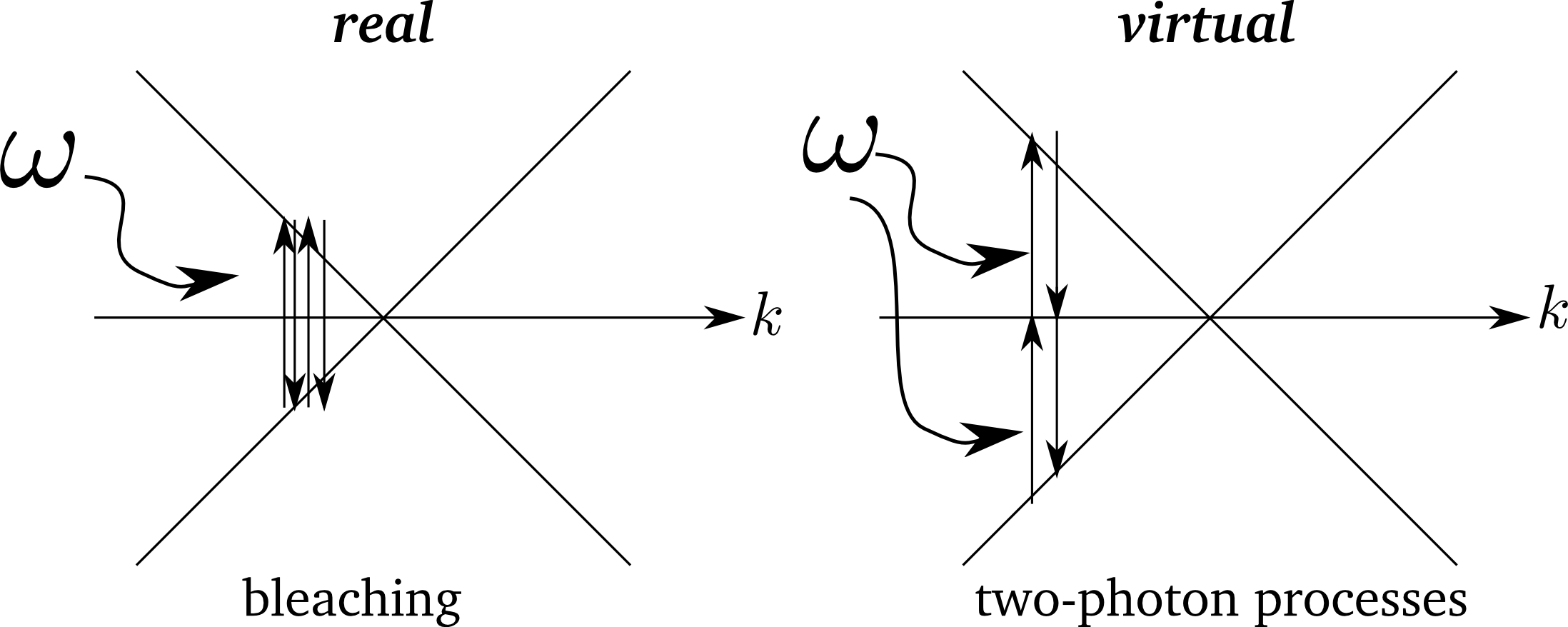
Figure 1: Third order optical processes in neutral graphene. Bleaching: two photons are absorbed with no virtual states involved. This process requires emission of a photon before the second one is absorbed. Resonant two-photon processes: a process where two photons are simultaneously absorbed involving a virtual state. In the case represented here, that state is located at zero energy. These type of processes also occur in traditional semiconductors, when the photon energy is smaller than the band-gap.Boyd

Analogously to $P_{x,1}$, the non-linear polarization $P_{x,3}$ is obtained from

$$P_{x,3}=iev_{F}g_{s}g_{v}\sum_{\bm{k}}\sin\theta[x_{3}(t)-x_{3}^{\ast}(t)]\,.$$ (40)

Replacing the expression for $x_{3}(t)$ in Eq. (40) we obtain (for neutral graphene at zero temperature)

$$P_{x,3}=\chi_{3}^{(\omega;bl)}\frac{E_{0}}{2}e^{-i\omega t}+\chi_{3}^{(\omega;2\gamma)}\frac{E_{0}}{2}e^{-i\omega t}+\mbox{h. c.}\,,$$ (41)

where $\chi_{3}^{(\omega;bl)}$ and $\chi_{3}^{(\omega;2\gamma)}$ are given by

$$\chi_{3}^{(\omega;bl)} = -\sigma_{0}{\cal W}_{i}\pi\alpha\frac{3v_{F}^{2}}{\hbar\omega^{2}\gamma^{2}}=-\sigma_{0}\beta_{\gamma}\,,$$ (42)

$$\chi_{3}^{(\omega;2\gamma)} = -\sigma_{0}{\cal W}_{i}\pi\alpha\frac{3v_{F}^{2}}{\hbar\omega^{3}}\frac{2\omega}{4\omega^{2}+\gamma^{2}}=-\sigma_{0}\beta_{\omega}/2\,,$$ (43)

with the respective imaginary parts being negligible in the regime $\hbar\gamma\ll\hbar\omega$. Note that both $\Re\chi_{3}^{(\omega;bl)}$ and $\Re\chi_{3}^{(\omega;2\gamma)}$ are negative due to saturate absorption. Also, both processes contribute to the imaginary part of the refraction index of graphene. We should note that the limit $\gamma\rightarrow 0$ can be taken in $\beta_{\omega}$ but not in $\beta_{\gamma}$. Indeed, $\Re\chi_{3}^{(\omega;bl)}$ and $\Re\chi_{3}^{(\omega;2\gamma)}$ correspond to two different physical processes typical of semiconductors:Boyd ; Meyer ; JiWei bleaching and virtual two-photon processes, as represented in Fig. 1. Each of these processes excite different electronic states.

For sake of completeness, we give the formula for the optical susceptibility due to three photon-absorption processes (i.e., the third-harmonic generation, $e^{i3\omega t}$, neglected above):

$$\chi_{3}^{(3\omega)}=\sigma_{0}{\cal W}_{i}\alpha\frac{3\pi v_{F}^{2}}{4\hbar\omega^{4}}\,.$$ (44)

The transmittance of free-standing graphene for normal incidence is obtained from

$${\cal T}=\frac{1}{|1+\chi(\omega)/(2\epsilon_{0}c)|^{2}}\,.$$ (45)

Taking into account the non-linear corrections, we have

$$\Re\chi(\omega)=\sigma_{0}(1-\beta_{\gamma})-\sigma_{0}\beta_{\omega}/2\,.$$ (46)

Since $\sigma_{0}/(2\epsilon_{0}c)=\pi\alpha$, the transmittance of neutral graphene at zero temperature is

$${\cal T}\simeq 1-\pi\alpha+\pi\alpha\beta_{\gamma}+\pi\alpha\beta_{\omega}/2\,,$$ (47)

where we have expanded Eq. (45) in the small parameter $\alpha$. Higher-order terms are negligible except for very high field intensities, that is, $\beta_{\gamma},\beta_{\omega}\gtrsim 1$. As expected, the non-linear contributions, $\beta_{\gamma}$ and $\beta_{\omega}$, induce a higher transparency of graphene, which increases as ${\cal W}_{i}$ also increases. [The imaginary part of $\chi(\omega)$, which we have neglected, gives a small correction to Eq. (47)—see the top right panel of Fig. 2 for the magnitude of the imaginary part of $\Im\chi(\omega)$ in the rotating wave approximation.]

It is important to realize that although the value of ${\cal W}_{i,\gamma}$, coming from $\beta_{\gamma}$, suggests that the absorption of graphene would saturate for moderate intensities, the much larger value of ${\cal W}_{i,\omega}$, coming from $\beta_{\omega}$, shows that graphene still absorbs light due to virtual resonant two-photon processes, even in the event of negligible bleaching. This is possible because, as already noted, the two processes –bleaching and the two-photon process– excite different electronic states. If light of broad spectral range is considered, instead of monochromatic light, the analysis will be more complex than the one presented here.

III.3 Approximate calculation of the non-linear susceptibility to all orders in the intensity of the field within the RWA

In the previous section we made a perturbative calculation of the non-linear optical susceptibility of graphene, up to first order in $\beta_{\gamma}$ and $\beta_{\omega}$. The exact calculation to all orders is not possible. However, an approximate calculation of the non-linear susceptibility valid to all orders in ${\cal W}_{i}$ can be obtained using the rotating wave approximation (RWA). Within the RWA, the solution of $X(t)=X$ is written as

$$X(t)=xe^{-i\omega t}+ye^{i\omega t}\,.$$ (48)

Inserting $X(t)$ in Bloch’s equations, we obtain

$$\dot{x}+(\gamma_{2}+i\epsilon-i\omega)x = i\frac{d_{\bm{k}}E_{0}}{2\omega}N\,,$$ (49)

$$\dot{y}+(\gamma_{2}+i\epsilon+i\omega)y = -i\frac{d_{\bm{k}}E_{0}}{2\omega}N\,,$$ (50)

$$\dot{N}+\gamma_{1}N \approx 4\frac{d_{\bm{k}}E_{0}}{2\omega}\Im(x-y)\,.$$ (51)

The explicit solution of the above set of equations is obtained by series resummation (assuming, for simplicity, $\gamma_{1}\approx\gamma_{2}\equiv\gamma$) and reads:

$$x = iN\frac{d_{\bm{k}}E_{0}}{2\omega}\frac{\gamma+i(\omega-2v_{F}k)}{(\omega-2v_{F}k)^{2}+\gamma^{2}}\,,$$ (52)

$$y = iN\frac{d_{\bm{k}}E_{0}}{2\omega}\frac{i(\omega+2v_{F}k)-\gamma}{(\omega+2v_{F}k)^{2}+\gamma^{2}}\,,$$ (53)

$$N = \frac{n_{0}}{1+\delta(k)}\,,$$ (54)

where $\delta(k)$ is given by

$$\delta(k,\theta) = \tilde{\beta}\gamma^{2}\sin^{2}\theta\left(\frac{1}{(\omega-2v_{F}k)^{2}+\gamma^{2}}\right.$$ (55)

$$+ \left.\frac{1}{(\omega+2v_{F}k)^{2}+\gamma^{2}}\right)\,,$$

and $\tilde{\beta}$ is defined as $\tilde{\beta}=(8/3)\beta_{\gamma}$.

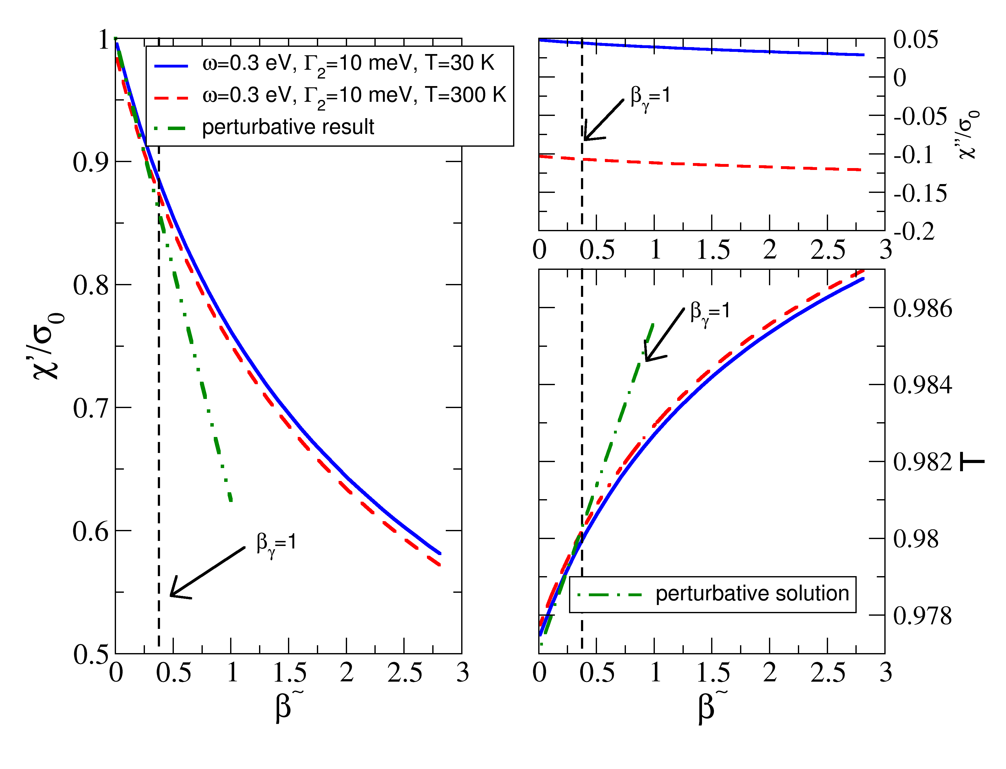
Figure 2: Optical susceptibility of graphene as function of $\tilde{\beta}$ within the RWA to all orders in ${\cal W}_{i}$. In the left panel we plot the real part of the optical susceptibility of graphene as function of the dimensionless parameter $\tilde{\beta}$ and in the right top panel we plot the imaginary part of the same quantity ($\mu=10^{-3}$ eV). The transmittance, ${\cal T}$, of light through graphene at normal incidence is plot in the right lower panel. The vertical dashed line corresponds to $\beta_{\gamma}=1$. The results are for $\hbar\omega=0.3$ eV and $\hbar\gamma=10$ meV and two different temperatures, $T=30,300$ K. The dashed-dotted line is the perturbative result given by Eqs. (46) and (47).

The calculation of the polarization follows the same procedure as before, and using

$$\int_{0}^{2\pi}d\theta\frac{\sin^{2}\theta}{1+a^{2}\sin^{2}\theta}=\frac{2\pi}{a^{2}}\frac{\sqrt{1+a^{2}}-1}{\sqrt{1+a^{2}}}\,,$$ (56)

we obtain

$$P(t)=\frac{E_{0}}{2}e^{-i\omega t}[\chi^{\prime}(\omega)+i\chi^{\prime\prime}(\omega)]+\mbox{c.c.}\,.$$ (57)

Considering zero temperature, with $\mu>0$ denoting the chemical potential, the susceptibility reads

$$\chi^{\prime}(\omega)=\sigma_{0}\frac{2}{\pi\tilde{\beta}}\int_{2\mu/\hbar\gamma}^{\infty}dy\frac{\sqrt{1+\tilde{\beta}g(y)}-1}{\sqrt{1+\tilde{\beta}g(y)}}\,,$$ (58)

and

$$\chi^{\prime\prime}(\omega)=\frac{\omega}{\gamma}\chi^{\prime}(\omega) - \sigma_{0}\frac{4}{\pi\tilde{\beta}}\frac{\omega}{\gamma}\int_{2\mu/\hbar\gamma}^{\infty}dy\frac{\sqrt{1+\tilde{\beta}g(y)}-1}{\sqrt{1+\tilde{\beta}g(y)}}\times$$ (59)

$$\times\frac{y^{2}}{1+y^{2}+\omega^{2}/\gamma^{2}}\,,$$

where

$$g(y)=\frac{1}{(y-\omega/\gamma)^{2}+1}+\frac{1}{(y+\omega/\gamma)^{2}+1}\,.$$

To zero order in $\tilde{\beta}$ we have the usual results (intra-band contributions excluded):

$$\chi^{\prime}(\omega)=\sigma_{0}\left(1+\sum_{s=\pm 1}\frac{s}{\pi}\arctan\frac{\hbar\omega-2\mu s}{\gamma\hbar}\right)\,,$$ (61)

and

$$\chi^{\prime\prime}(\omega)=-\sigma_{0}\frac{1}{2\pi}\ln\frac{(2\mu+\hbar\omega)^{2}+\hbar\gamma^{2}}{(2\mu-\hbar\omega)^{2}+\hbar\gamma^{2}}\,.$$ (62)

To first order in $\tilde{\beta}$ and for neutral graphene at zero temperature, we obtain for the real part of the susceptibility the approximate result

$$\chi^{\prime}(\omega)\approx-\sigma_{0}\beta_{\gamma}-\sigma_{0}\beta_{\omega}\,.$$ (63)

It is apparent from Eqs. (46) and (63) that the contribution coming from the bleaching process is exact [first term in Eq. (63)], whereas the contribution from virtual two-photon process is overestimated by a factor of two in the RWA.

In Fig. 2 we compare the perturbative (dashed-dotted line) results given by Eqs. (46) and (47), left and right-bottom panels, respectively, with the RWA, valid for an arbitrary value of ${\cal W}_{i}$ (we plot results for two different temperatures: $T=30$ K, solid line, $T=300$ K dashed line). Clearly, the perturbative result and the RWA calculation agree well up to $\beta_{\gamma}=1$, which sets perturbation theory validity limit. Beyond that value a non-perturbative approach is necessary and one has to rely on the RWA for drawing quantitative conclusions.

IV An efficient graphene-based photodetector

In this section we describe the absorption of light by a device composed of optical cavities and a single graphene sheet. Only the linear optical susceptibility will be considered, except when the light intensity inside the cavity is of the order of ${\cal W}_{i,\gamma}$ (we remark that for telecommunication devices and photodetectors this will hardly be the case).

IV.1 Properties of a mirror and of an empty optical cavity

We start with the well-known case of an empty optical cavity. This allow us to introduce important concepts and fix the notation. The scattering matrix of a partially-silvered mirror is characterized by two pairs of reflectance and transmittance coefficients; such a mirror is shown in Fig. 3.

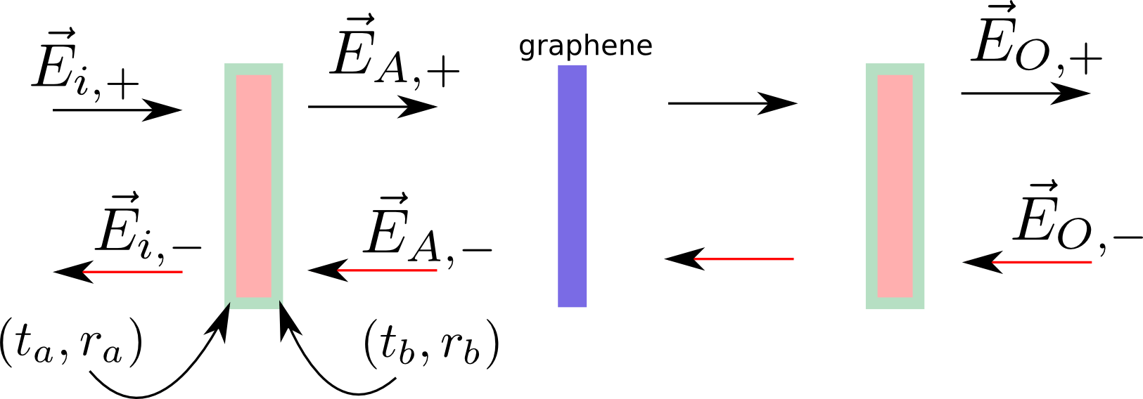
Figure 3: Graphene inside an optical cavity. The cavity is defined by two equal mirrors with reflectance amplitudes $r_{a}$ and $r_{b}$, and transmittance amplitudes $t_{a}$ and $t_{b}$.

The $S-$matrix relates the amplitudes of the incoming waves, $E_{i,+}$ and $E_{A,-}$, to the amplitudes of the outgoing waves, $E_{i,-}$ and $E_{A,+}$, according to

$$\left[\begin{array}[]{c}E_{A,+}\\ E_{i,-}\end{array}\right]=\left[\begin{array}[]{cc}t_{a}&r_{b}\\ r_{a}&t_{b}\end{array}\right]\left[\begin{array}[]{c}E_{i,+}\\ E_{A,-}\end{array}\right]\,.$$ (64)

On the other hand, the transfer matrix $M_{m}$ relates the fields on the two sides of the mirror according to

$$\left[\begin{array}[]{c}E_{A,+}\\ E_{A,-}\end{array}\right]=\frac{1}{t_{b}}\left[\begin{array}[]{cc}t_{a}t_{b}-r_{a}r_{b}&r_{b}\\ -r_{a}&1\end{array}\right]\left[\begin{array}[]{c}E_{i,+}\\ E_{i,-}\end{array}\right]\,.$$ (65)

Let us now discuss few properties obeyed by the reflectance and transmittance amplitudes.Saleh From the conservation of the energy flux

$$|E_{i,+}|^{2}-|E_{i,-}|^{2}=|E_{A,+}|^{2}-|E_{A,-}|^{2}$$ (66)

we find

$$|t_{a}|^{2}+|r_{a}|^{2}=1\,,$$ (67)

$$|t_{b}|^{2}+|r_{b}|^{2}=1\,,$$ (68)

$$t_{a}r_{b}^{\ast}=-t_{b}^{\ast}r_{a}\,.$$ (69)

From $t_{a}r_{b}^{\ast}=-t_{b}^{\ast}r_{a}$ we find

$$|t_{a}|^{2}=|t_{b}|^{2}\frac{|r_{a}|^{2}}{|r_{b}|^{2}}\,,$$ (70)

which can be used to show that $|t_{a}|=|t_{b}|$ and $|r_{a}|=|r_{b}|$. Furthermore, the determinant of the transfer matrix reads $\mbox{det\,}M_{m}=t_{a}/t_{b}$, implying that $|\mbox{det\,}M_{m}|=|t_{a}/t_{b}|=1$. For systems with inversion symmetry, we can write $t_{a}=t_{b}=t$ and $r_{a}=r_{b}=r$. Thus, the $S-$matrix reads

$$S=\left[\begin{array}[]{cc}t&r\\ r&t\end{array}\right]\,,$$ (71)

and the transfer matrix can written as

$$M_{m} = \frac{1}{t}\left[\begin{array}[]{cc}t^{2}-r^{2}&r\\ -r&1\end{array}\right]=\left[\begin{array}[]{cc}t+|r|^{2}/t^{\ast}&r/t\\ -r/t&1/t\end{array}\right]$$ (76)

$$= \left[\begin{array}[]{cc}1/t^{\ast}&r/t\\ r^{\ast}/t^{\ast}&1/t\end{array}\right]\,.$$ (79)

Writing $r=|r|e^{i\alpha_{r}}$ and $t=|t|e^{i\alpha_{t}}$, the relation $tr^{\ast}=-t^{\ast}r$ implies that $e^{i2(\alpha_{r}-\alpha_{t})}=-1$, that is, $\alpha_{r}=\alpha_{t}\pm\pi/2$. Using these last relations, $M_{m}$ can be written as

$$M_{m}=\frac{1}{t}\left[\begin{array}[]{cc}-1&-|r|\\ |r|&1\end{array}\right]\,.$$ (80)

If two of these mirrors are separated by a distance $L$ we have to define the transfer matrix associated with the free propagation from the first to the second mirror. Since

$$E_{+}(x,t) = E_{+}e^{i(kx-\omega t)}\,,$$ (81)

$$E_{-}(x,t) = E_{-}e^{-i(kx+\omega t)}\,,$$ (82)

then at a distance $L$ to the right the $E_{+}(x+L,t)$ has an extra phase of $e^{ikL}$ whereas the $E_{-}(x+L,t)$ has an extra phase of $e^{-ikL}$. Thus we have

$$\left[\begin{array}[]{c}E_{A,+,L}\\ E_{A,-,L}\end{array}\right]=\left[\begin{array}[]{cc}e^{ikL}&0\\ 0&e^{-ikL}\end{array}\right]\left[\begin{array}[]{c}E_{A,+}\\ E_{A,-}\end{array}\right]\,,$$ (83)

or

$$\left[\begin{array}[]{c}E_{A,+}\\ E_{A,-}\end{array}\right]=\left[\begin{array}[]{cc}e^{-ikL}&0\\ 0&e^{ikL}\end{array}\right]\left[\begin{array}[]{c}E_{A,+,L}\\ E_{A,-,L}\end{array}\right]\,,$$ (84)

where $E_{A,+/-,L}$ represents the amplitude of the forward/backward propagating field at the right end of the cavity and the matrix

$$M_{f}(L)=\left[\begin{array}[]{cc}e^{-ikL}&0\\ 0&e^{ikL}\end{array}\right]$$ (85)

defines the free propagation to the right. Then, the transmitted field through two mirrors at a distance $L$ from each other follows from

$$\left[\begin{array}[]{c}E_{i,+}\\ E_{i,-}\end{array}\right]=M_{m}\cdot M_{f}(L)\cdot M_{m}\left[\begin{array}[]{c}E_{O,+}\\ E_{O,-}\end{array}\right]\,.$$ (86)

Explicitly, we have

$$E_{i,+}=\frac{e^{-ikL}}{(t^{\ast})^{2}}[1-(r^{\ast})^{2}e^{2ikL}]E_{O,+}\,,$$ (87)

writing $r^{\ast}=|r|^{-i\alpha_{r}}$ we obtain

$${\cal T}\equiv\frac{|E_{O,+}|^{2}}{|E_{i,+}|^{2}}=\frac{|t|^{4}}{|t|^{4}+4|r|^{2}\sin^{2}(kL)}\,,$$ (88)

since $\alpha_{r}=\pi$, as implied by Fresnel equations. Thus we have perfect transmission for $kL=n\pi$ or $\lambda=2L/n$, with $n=1,2,3,\ldots$. The longest wavelength for which perfect transmission is possible is $\lambda=2L$. It is straightforward to show that the transmission is strongly suppressed for other choices of $kL$. For instance, when $kL$ is a multiple of $\pi/2$, we have

$${\cal T}=\frac{|t|^{4}}{|t|^{4}+4|r|^{2}}\approx\frac{|t|^{4}}{4|r|^{2}}\ll 1\,,$$ (89)

In the above, we have admitted high-quality mirrors, $|r|\gg|t|$, to simplify the denominator.

The introduction of a graphene sheet inside the cavity leads to light absorption and the relation (88) is modified. In the following section, we demonstrate how to explore the physics of an optical cavity to devise an efficient graphene-based photodetector.

IV.2 Graphene in an optical cavity

We describe the transmission of light through a graphene sheet inside an optical cavity taking into account the linear optical-susceptibility of graphene.

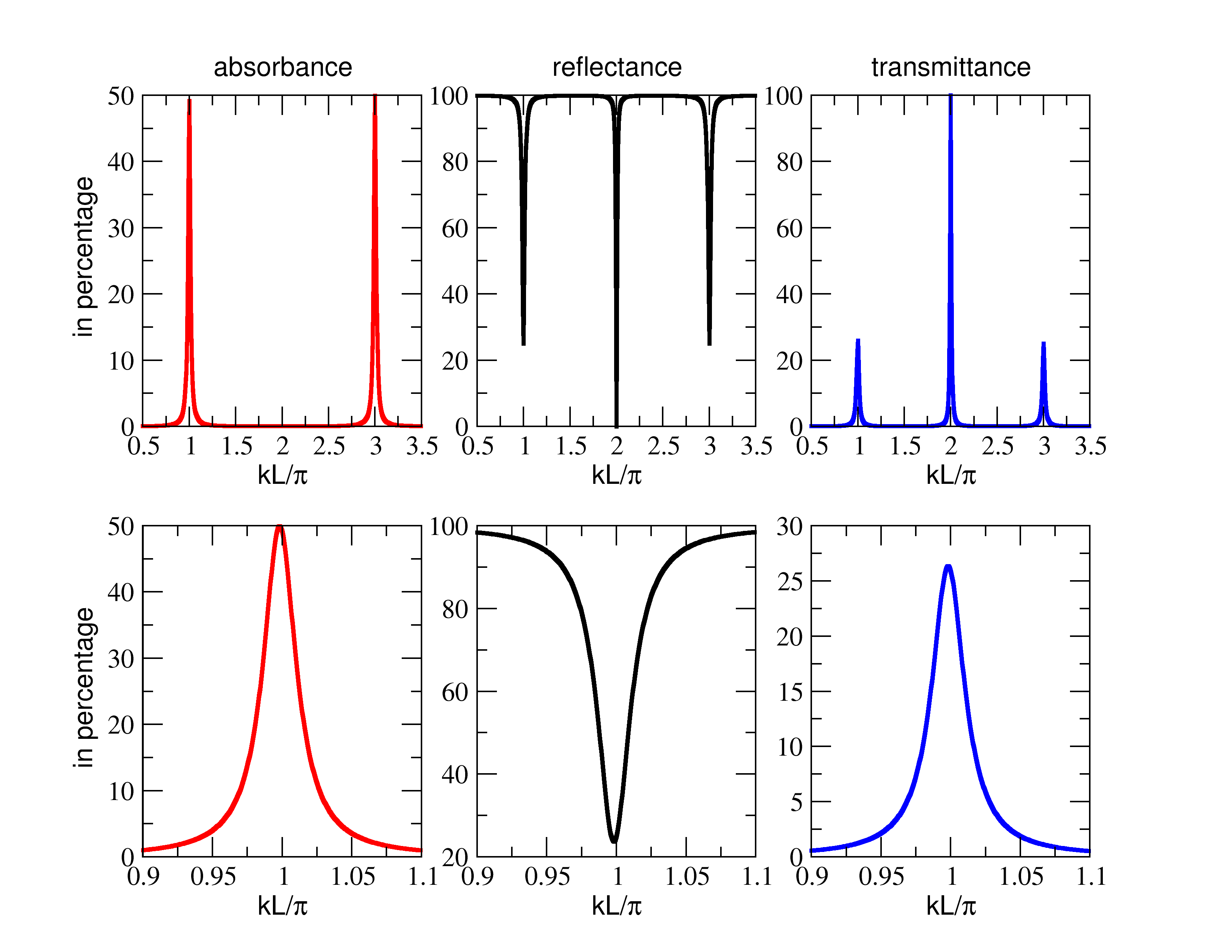
Figure 4: Transmission spectrum for a Fabry-Pérot cavity with graphene $L/2$. The mirror transmittance is $t^{2}=0.045$. If we tale $\lambda=1000$ nm, then the range $kL/\pi$ in the lower panels spans the wavelengths from $\lambda=900$ nm to $\lambda=1100$ nm. We have taken $\hbar\gamma=7$ meV and $T=300$ K. Regarding the choice of $\lambda$, we note that the first HeNe laser was working at the spectral wavelength of 1150 nm, that is in the infrared.

We write the transfer matrix of graphene asEOM

$$M_{g}=\left[\begin{array}[]{cc}1+\eta&\eta\\ -\eta&1-\eta\end{array}\right]\,,$$ (90)

where $2\eta=Z_{0}\chi(\omega)$, with $\eta=\eta^{\prime}+i\eta^{\prime\prime}$, and $Z_{0}\simeq 376.7$ $\Omega$ is the vacuum impedance. For neutral graphene at zero temperature $\eta$ is essentially a real number for frequencies below the visible spectral range. The transmission through the cavity with graphene at position $x_{g}$ and the second mirror at position $x=L$ follows from

$$\left[\begin{array}[]{c}E_{i,+}\\ E_{i,-}\end{array}\right]=M_{m}\cdot M_{f}(x_{g})\cdot M_{g}\cdot M_{f}(L-x_{g})\cdot M_{m}\left[\begin{array}[]{c}E_{O,+}\\ E_{O,-}\end{array}\right]\,.$$ (91)

The matrix

$$M=M_{m}\cdot M_{f}(x_{g})\cdot M_{g}\cdot M_{f}(L-x_{g})\cdot M_{m}$$ (92)

is the full transfer matrix of the device. The transmittance and the reflectance are defined as

$${\cal T} = \frac{1}{|M_{11}|^{2}}\,,$$ (93)

$${\cal R} = \left|\frac{M_{21}}{M_{11}}\right|^{2}\,,$$ (94)

respectively, and $M_{11}$ and $M_{12}$ denote the matrix elements of $M$. We note that ${\cal R}\neq 1-{\cal T}$ due to absorption by graphene (we are assuming lossless mirrors). The absorbance is defined as ${\cal A}=1-{\cal R}-{\cal T}.$

For $x_{g}=L/2$ we have

$${\cal T} = \frac{|t|^{4}}{|1+\eta-2\eta|r|e^{ikL}-(1-\eta)|r|^{2}e^{2ikL}|^{2}}\,,$$ (95)

$${\cal R} = \frac{|(1+\eta)|r|-\eta(1+|r|^{2})e^{ikL}-(1-\eta)|r|e^{2ikL}|^{2}}{|1+\eta-2\eta|r|e^{ikL}-(1-\eta)|r|^{2}e^{2ikL}|^{2}}\,.$$ (96)

In the limit $r\rightarrow 0$ we recover the well known result, ${\cal T}=1/|1+\eta|^{2}$ [see also Eq. (45)] and ${\cal R}=|\eta|^{2}/|1+\eta|^{2}$.stauberFullSigma

The effect of graphene in the cavity is to reduce the intensity of the odd-orders ($n=1,3,5,\ldots$) of perfect transmission in the otherwise perfect cavity. From Fig. 4 it is clear that the reduction of transmission of the odd orders is divided between reflection and absorption, the latter taking the majority of the incoming power. The transmission is still unity for even-orders ($n=2,4,6,\ldots$). In Fig. 5 we show the dependence of the absorbed power as function of the transmittance $t^{2}$ of a mirror. Clearly, this dependence is not monotonous, displaying a maximum around $t^{2}\simeq 0.045$. An analytical expression for the value of $t^{2}$ for which the absorption is maximum can be readily obtained from Eq. (95).

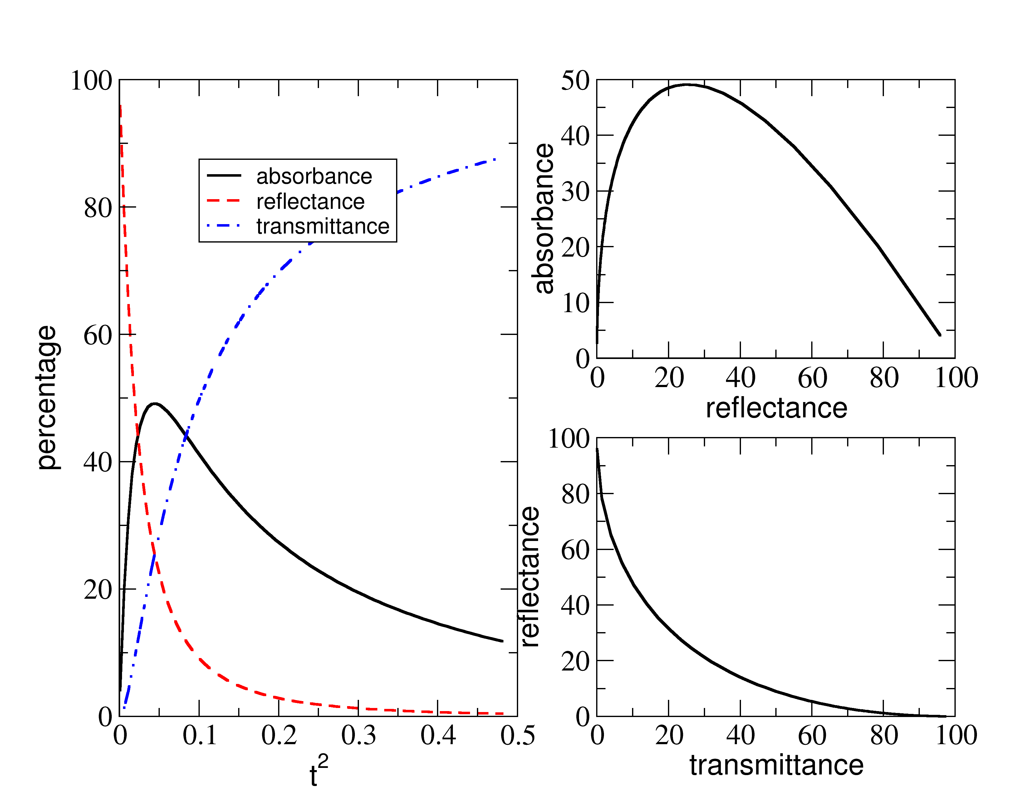
Figure 5: Absorbance of graphene for the single cavity system (see Fig. 3). Left: Absorbance as function of mirror transmittance $t^{2}\in[0,0.5]$. Top right: Absorbance of graphene as function of reflectance. Bottom right: reflectance of graphene as function of transmittance. The calculations assumed $T=300$ K.

IV.3 Double optical cavity

The goal of the present section is to discuss a device able to enhance light absorption relatively to the single cavity system discussed above. To that end we consider a graphene sheet inside an optical cavity of length $L$ (as in the previous section) followed by an empty quarter-wavelength cavity, as represented in Fig. 6.

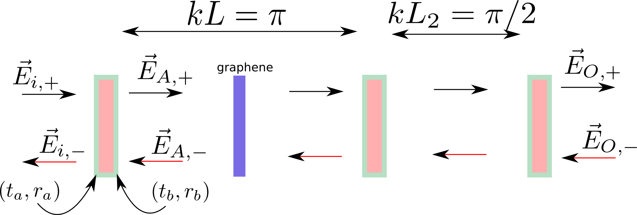
Figure 6: The double cavity system: Light impinges from the left-hand side. The second cavity has half the length of the first cavity, $L_{2}=L/2$.

Placing graphene at the middle of the first cavity and choosing its length $L$ such that $L=\lambda/2$, where $\lambda$ is the wavelength of the light, we expect that graphene will present an enhanced absorption at this wavelength, at least for a cavity with a high finesse. This intuitive picture is developed from considering, as a rough approximation, the formation of standing waves within the cavity having their maximum amplitudes at the center of the cavity. This picture in confirmed by simulations, as shown in Fig. 4. Also from Fig. 5 it is clear that there is an optimal value of $t^{2}$ for which the absorption can be as high as 50% (the quantitative results are robust for small changes graphene’s position relatively to the center of the cavity).

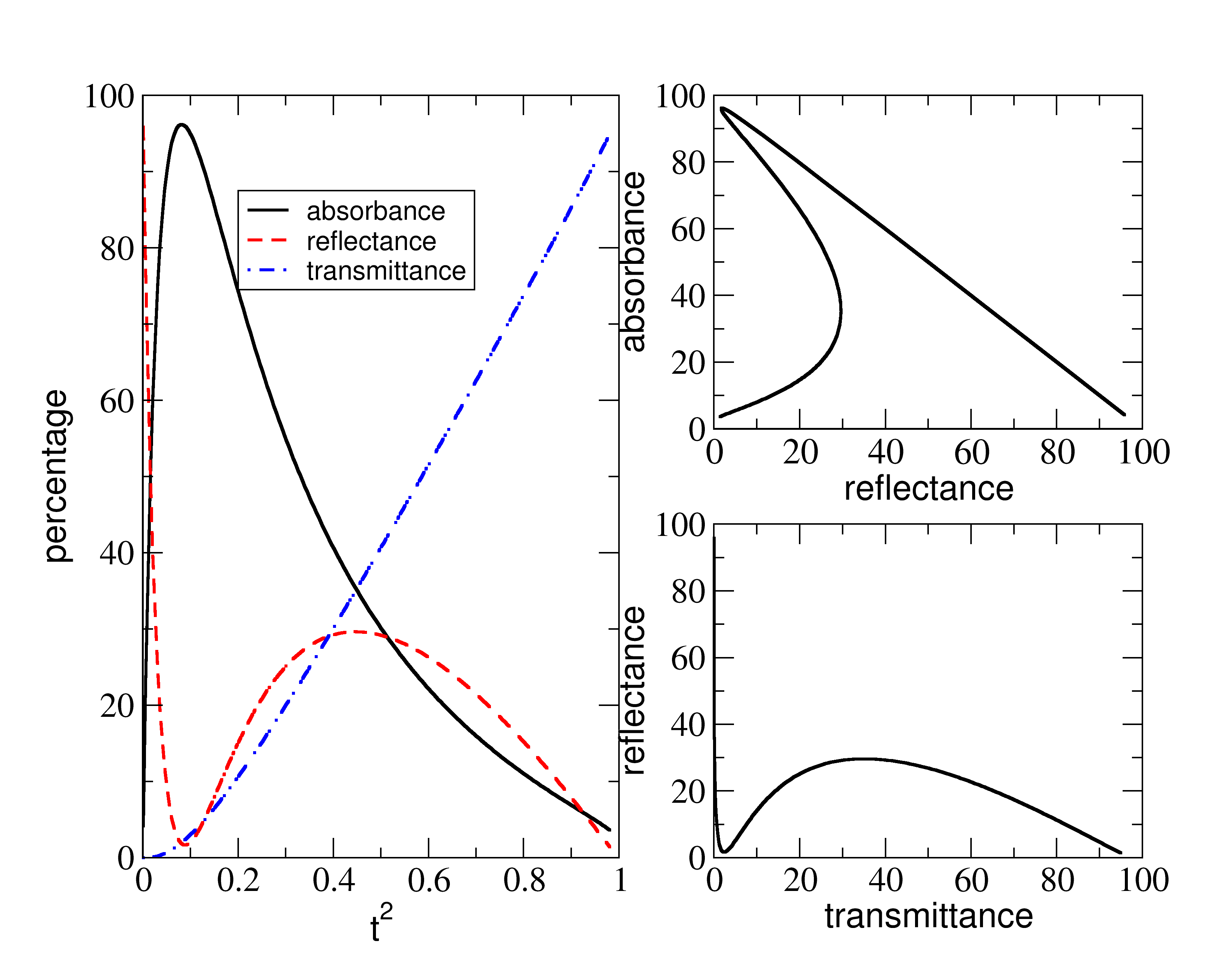
Figure 7: Absorbance of graphene for the double cavity setup (see Fig. 6). Left: Absorbance as function of mirror transmittance $t^{2}\in[0,1]$. Top right: Absorbance as function of reflectance. Bottom right: Reflectance as function of transmittance. The calculations assumed $T=300$ K.

The absorbed intensity can be pushed up to $\simeq 100\%$ by building an optical cavity containing graphene, followed by an empty quarter-wavelength cavity, that is, a cavity with length $L_{2}$ such that $L_{2}=\lambda/4$. This setup leads to an enhancement of the absorption, which is about twice as large as that of the single cavity setup, as can be seen in the left panel of Fig. 7. The dependence of the absorption on the wavelength is shown in Fig. 8.

A physical qualitative argument for the absorption enhancement effect in a double cavity is reminiscent of a quantum particle in a box with a permeable wall. Let us consider first a box with origin at $x=0$ and length $L+L/2$. A wall is located at $x=L$. If the wall is impermeable, the fundamental mode of the the first box is $\lambda=2L$ and that of the second box is $\lambda=L$. If the wall becomes permeable the two modes hybridize and in the ground state the probability density grows in the first box at the expenses of the probability density in the second box. Translating this into our problem, the quarter wavelength cavity interference between the wave reflected by the third mirror and the forward propagating wave effectively suppresses the transmission at wavelengths $\lambda=2L$, forcing the photon to spend more time in the first cavity, and thus increasing the absorption by the graphene sheet.

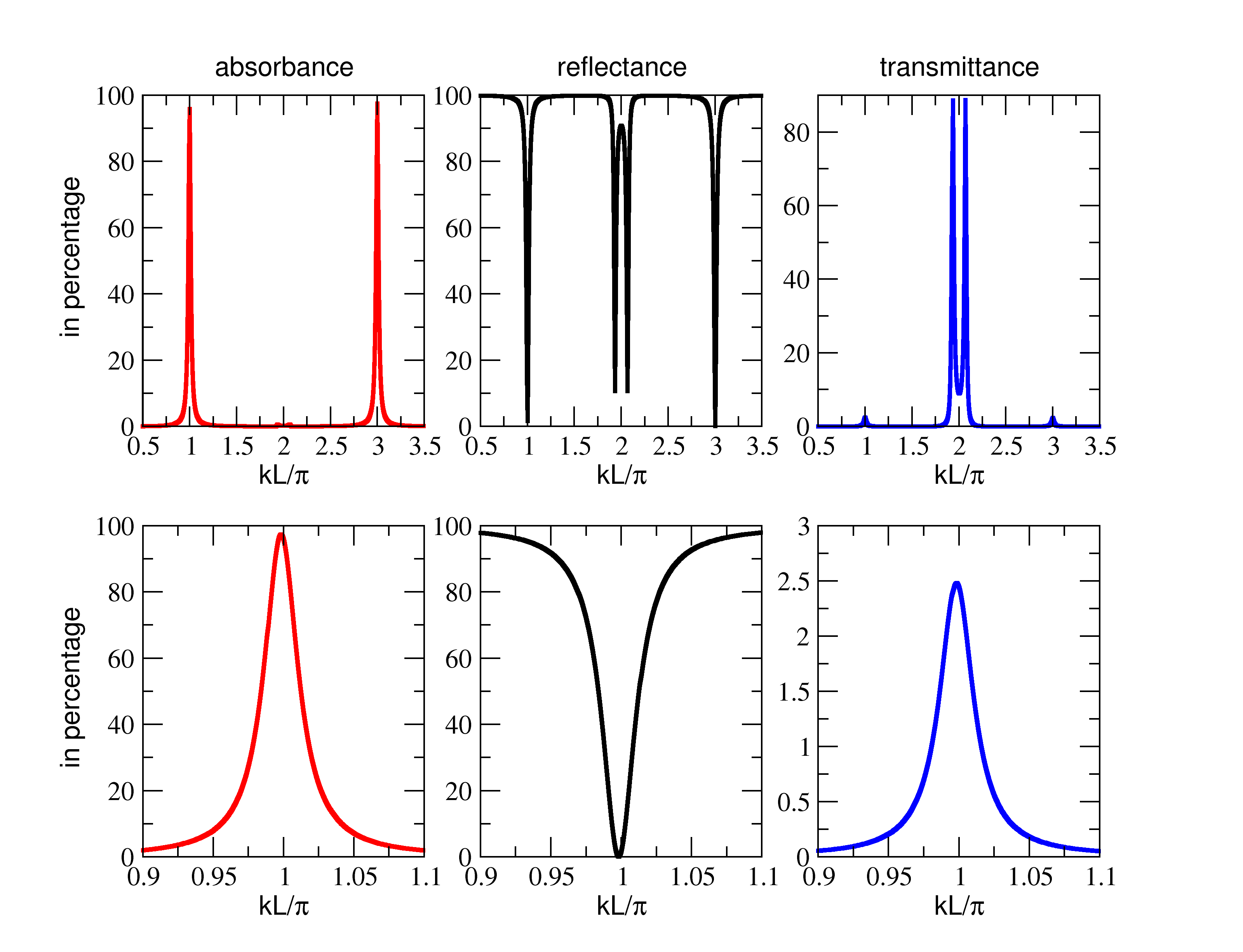
Figure 8: Absorbance as function of $kL/\pi=2L/\lambda$ for the double cavity system ($t^{2}=0.09$). If we consider $\lambda=1000$ nm, then the range of $kL/\pi$ in the lower panels spans the wavelengths from $\lambda=900$ nm to $\lambda=1100$ nm.

It is worth stressing that the maximum of absorption takes place for cavities with $|t|^{2}\simeq 0.1$, a convenient figure from the point of view of micro-fabrication since not much effort has to be put on building highly reflective mirrors.

From a theoretical point of view, the calculation of the properties of the two coupled cavities follows from the transfer matrix method, reviewed in IV.2. As in Eq. (91), the incoming and outgoing field amplitudes are related as

$$\left[\begin{array}[]{c}E_{i,+}\\ E_{i,-}\end{array}\right]=M_{{\rm cav}}\left[\begin{array}[]{c}E_{O,+}\\ E_{O,-}\end{array}\right]\,,$$ (97)

where the transfer matrix of the two cavities is given by

$$M_{{\rm cav}}=M_{m}\cdot M_{f}(x_{g})\cdot M_{g}\cdot M_{f}(L-x_{g})\cdot M_{m}\cdot M_{f}(L_{2})\cdot M_{m}\,.$$ (98)

In Figs. 7 and 8 we have considered $x_{g}=L/2$. In this case the field amplitudes for $\lambda=(2n+1)L/2$ (with $n=0,1,2,\ldots$) have a maximum at the center of the cavity. As for the case of the single cavity, it is possible to derive analytical expressions for both ${\cal T}$ and ${\cal R}$; we obtain

$$\mathcal{T}=\frac{|t|^{6}}{\left|1+\eta+\Lambda_{1}e^{ikL}+\Lambda_{2}e^{2ikL}+\Lambda_{3}e^{3ikL}\right|^{2}}\,.$$ (99)

In the above, $\Lambda_{1}=-[\eta(2+|r|)+|r|]|r|$, $\Lambda_{2}=[\eta(1+|r|+|r|^{2})-|r|]|r|$ and $\Lambda_{3}=(1-\eta)|r|^{2}$, and

$$\mathcal{R}=\frac{\mathcal{T}}{|t|^{6}}\left|(1+\eta)|r|+\Delta_{1}e^{ikL}+\Delta_{2}e^{2ikL}+\Delta_{3}e^{3ikL}\right|^{2}\,,$$ (100)

with $\Delta_{1}=-[\eta(1+|r|^{2}+|r|^{3})+|r|^{3}]$, $\Delta_{2}=(\eta-1+2|r|\eta)|r|$ and $\Delta_{3}=(1-\eta)|r|$. As before, taking the limit $r\rightarrow 0$ we recover the well known values for ${\cal T}$ and ${\cal R}$ in the absence of mirrors.

It is interesting to note the hysteresis in the absorbance as function of the reflected power —some values of the reflectance admit three possible absorbances; see top right panel of Fig. 7. Each point on the ${\cal A}$ versus $\mathcal{R}$ curve corresponds to a given value of the mirror transmittance, $|t|^{2}$, which therefore can be viewed as an external driving field.

Finally, we note that about 100% absorption can also be obtained for a single cavity if the second mirror reflects 100% of the impinging light. The curves ${\cal A}$, ${\cal R}$, and ${\cal T}$ as function of $t^{2}$ are different in this case, however, from those given above; in particular, ${\cal A}$ shows no hysteresis (see note after Conclusions section).micro

V Conclusions

In the present article, we have developed the theory a graphene-based photodetector with nearly 100% efficiency for photon frequencies around a predefined value. The proposed setup is general and should work in a vast spectral range.

We have also clarified the role of the non-linear optical susceptibility in determining the properties of the cavity-graphene system. We have shown that non-linear terms are irrelevant for moderate light intensities.

The most efficient photodetector is built from combining a half-wavelength cavity (size $L=\lambda/2$) followed by a second quarter-wave length cavity (size $L_{2}=\lambda/4$). This system improves the absorption by a factor of two relatively to the single cavity. As noted above, the two-cavities photodetector has about the same absorbance as a single cavity with the second mirror having zero transmittance and the first one having $t^{2}\simeq 0.9$.

If real-time control of the mirrors transmittance is feasible, then it will be possible to obtain hysteresis in the absorbance for the same reflectance value. Whether this can be used as an optical logical gate is so far unclear and will be left for future research.

Although in the schematic figures for the cavities graphene appears floating in the air, in practical terms it will be deposited on a dielectric. The mirrors can also be made of dielectric materials, the so called Bragg mirrors. There are computer codes for simulating mirrors with the prescribed optimal value of $t^{2}$ given in the text. The setup itself can be built by micro-fabrication using standard techniques.

Note: during the final state of writing, we became aware of an experimental paper, entitled “Microcavity-integrated graphene photodetector”. In that work a single cavity detector has been built.micro Our theory is a full analytical account of the physics of two similar devices, one of them having the same theoretical efficiency as the device of that paper but a different qualitative response as function of the amplitude $t^{2}$.

A.F. acknowledges FCT Grant No. SFRH/BPD/65600/2009. N.M.R.P. and R.M.R. acknowledge Fundos FEDER, through the Programa Operacional Factores de Competitividade - COMPETE and by FCT under Project No. Past-C/FIS/UI0607/2011. T.S. acknowledges FCT Grant No. PTDC/FIS/101434/2008 and FIS2010-21883-C02-02 (MICINN).

References

- (1) A. H. Castro Neto, F. Guinea, N. M. R. Peres, K. S. Novoselov, and A. K. Geim, Rev. Mod. Phys. 81, 109 (2009).
- (2) R. R. Nair, P. Blake, A. N. Grigorenko, K. S. Novoselov, T. J. Booth, T. Stauber, N. M. R. Peres, and A. K. Geim, Science 320, 1308 (2008).
- (3) N. M. R. Peres, Rev. Mod. Phys. 82, 2673 (2010).
- (4) F. Xia, T. Mueller, Y. ming Lin, A. Valdes-Garcia, and P. Avouris, Nature Nanotechnology 4, 839 (2009).
- (5) N. M. R. Peres, F. Guinea, and A. H. Castro Neto, Phys. Rev. B 73, 125411 (2006).
- (6) D. S. L. Abergel, A. Russell, and V. I. Fal’ko, Appl. Phys. Lett. 91, 063125 (2007).
- (7) V. P. Gusynin, S. G. Sharapov, and J. P. Carbotte, Int. Jour. of Mod. Phys. B 21, 4611 (2007).
- (8) L. A. Falkovsky, and S. S. Pershoguba, Phys. Rev. B 76, 153410 (2007).
- (9) L. A. Falkovsky, and A. A. Varlamov, Eur. Phys. J. B 56, 281 (2007).
- (10) F. H. L. Koppens, D. E. Chang, and F. J. G. de Abajo, Nano Lett. 11, 3370 (2011).
- (11) A. H. Castro Neto and K. Novoselov, Mater. Express 1, 10 (2011).
- (12) L. Yang, J. Deslippe, C. Park, M. L. Cohen, and S. G. Louie, Phys. Rev. Lett. 103, 186802 (2009).
- (13) A. H. Castro Neto and K. Novoselov, Rep. Prog. Phys. 74, 082501 (2011).
- (14) S. Thongrattanasiri, F. H. L. Koppens, and F. J. García de Abajo, Phys. Rev. Lett. 108, 047401 (2012).
- (15) E. Ozbay, Science 311, 189 (2006).
- (16) Y. V. Bludov, M. I. Vasilevskiy, and N. M. R. Peres, EPL 92, 68001 (2010).
- (17) L. Ju, B. Geng, J. Horng, C. Girit, M.Martin, Z. Hao, H. A. Bechtel, X. Liang, A. Zettl, Y. R. Shen, and F. Wang, Nature Nano. 6, 630 (2011).
- (18) T. Echtermeyer, L. Britnell, P. Jasnos, A. Lombardo, R. Gorbachev, A. Grigorenko, A. Geim, A. Ferrari, and K. Novoselov, Nature Comm. 2, 458 (2011).
- (19) H. Haug, and S. W. Koch, Quantum Theory of the Optical and Electronic Properties of Semiconductors, 4th ed. (World Scientific, 2003).
- (20) T. Winzer, A. Knorr, and E. Malic, Nano Lett. 10, 4839 (2010).
- (21) N. M. R. Peres, R. M. Ribeiro, A. H. Castro Neto, Phys. Rev. Lett. 105, 055501 (2010).
- (22) A. Ferreira, J. Viana-Gomes, Y. V. Bludov, V. M. Pereira, N. M. R. Peres, and A. H. Castro Neto, Phys. Rev. B 84, 235410 (2011).
- (23) W. Schäfer, and M.Wegener, Semiconductor Optics and Transport Phenomena (Springer, 2002).
- (24) T. Stauber, N. M. R. Peres, and A. K. Geim, Phys. Rev. B 78, 085432 (2008).
- (25) V. M. Pereira, R. M. Ribeiro, N. M. R. Peres, and A. H. Castro Neto, EPL 92, 67001 (2010).
- (26) O. Nakada, J. Phys. Soc. Jpn. 15, 2280 (1960).
- (27) R. W. Boyd, Nonlinear Optics, 2nd ed. (Academic Press, 2003).
- (28) V. Nathan, A. H. Guenther, and S. S. Mitra, J. Opt. Soc. Am. B 2, 294 (1985).
- (29) H. Yang, X. Feng, Q. Wang, H. Huang, W. Chen, A. T. S. Wee, and W. Ji, Nano Lett. 11, 2622 (2011).
- (30) E. A. Saleh, and M. C. Teich, Fundamentals of Photonics, 2nd ed. (Wiley-Interscience, 2007).
- (31) M. Furchi, A. Urich, A. Pospischil, G. Lilley, K. Unterrainer, H. Detz, P. Klang, A. M. Andrews, W. Schrenk, G. Strasser, and T. Mueller, pre-print: arXiv:1112.1549 (2011).