Revisit to the tail asymptotics of the double QBD process: Refinement and complete solutions for the coordinate and diagonal directions

Abstract

We consider a two dimensional skip-free reflecting random walk on a nonnegative integer quadrant. We are interested in the tail asymptotics of its stationary distribution, provided its existence is assumed. We derive exact tail asymptotics for the stationary probabilities on the coordinate axis. This refines the asymptotic results in the literature, and completely solves the tail asymptotic problem on the stationary marginal distributions in the coordinate and diagonal directions. For this, we use the so-called analytic function method in such a way that either generating functions or moment generating functions are suitably chosen. The results are exemplified by a two node network with simultaneous arrivals.

1 Introduction

We are concerned with a two dimensional reflecting random walk on a nonnegative integer quadrant, which is the set of two dimensional vectors $(i,j)$ such that $i,j$ are nonnegative integers. We assume that it is skip free in all directions, that is, its increments in each coordinate direction are at most one in absolute value. The boundary of the quadrant is partitioned into three faces, the origin and the two coordinate axes in the quadrant. We assume that the transition probabilities of this random walk is homogeneous on each boundary face, but they may change on different faces or the interior of the quadrant, that is, inside of the boundary.

This reflecting random walk is referred to as a double quasi-birth-and-death process, a double QBD process for short, in Miyazawa 2009 . This process can be used to describe a two node queueing network under various setting such as server collaboration and simultaneous arrivals and departures, and its stationary distribution is important for the performance evaluation of such a network model. The existence of the stationary distribution, that is, stability, is nicely characterized, but the stationary distribution is hard to analytically get except for some special cases. Because of this as well as its own importance, research interest has been directed to its tail asymptotics.

Until now, the tail asymptotics for the double QBD have been obtained in terms of its modelling primitives under the most general setting in Miyazawa Miyazawa 2009 , while less explicit results have been obtained for more general two dimensional reflecting random in Borovkov and Mogul’skii BM 2001 . Foley and McDonald FM 2005a ; FM 2005b studied the double QBD under some limitations. Recently, Kobayashi and Miyazawa KM 2011 modified the double QBD process in such a way that upward jumps may be unbounded, and studied its tail asymptotics. This process, called a double $M/G/1$ type, includes the double QBD process as a special case. For special cases such as tandem and priority queues, the tail asymptotics have been recently investigated in Guillemin and Leeuwaarden Guillemin-Leeuwaarden 2011 and Li and Zhao Li-Zhao 2009 ; Li-Zhao 2011a . Recently, Li and Zhao Li-Zhao 2011b challenged the general double QBD (see Additional note at the end of this section).

The tail asymptotic problems have also been studied for a semi-martingale reflecting Brownian motion, SRBM for short, which is a continuous time and state counterpart of a reflecting random walk. For the two dimensional SRBM, the rate function for large deviations has been obtained under a certain extra assumption in Avram Dai and Hasenbein Avram-Dai-Hasenbein 2001 . Dai and Miyazawa Dai-Miyazawa 2011a derived more complete answers but for the stationary marginal distributions.

Thus, we now have many studies on the tail asymptotics for two dimensional reflecting and related processes (see, e.g., Miyazawa 2011 for survey). Nevertheless, there still remain many problems unsolved even for the double QBD. The exact tail asymptotics of the stationary marginal distributions in the coordinate directions are one of such problems. Here, a sequence of nonnegative numbers $\{p(n);n=0,1,2\}$ is said to have exact tail asymptotic $\{h(n);n=0,1,\ldots\}$ if their ratio $p(n)/h(n)$ converges to a positive constant as $n$ goes to infinity. We also write this asymptotic as

$$p(n)\sim h(n)$$

We will find $h(n)=n^{\kappa}a^{-n}$ or $n^{\kappa}(1+b(-1)^{n})a^{-n}$ with constants $\kappa=-\frac{3}{2},-\frac{1}{2},0,1$, $a>1$ and $|b|\leq 1$ for the marginal distributions (also for the stationary probabilities on the boundaries).

We aim to completely solve the exact tail asymptotics of the stationary marginal distributions in the coordinate and diagonal directions, provided the stationary distribution exists. It is known that the tail asymptotics of the stationary probabilities on each coordinate axis are a key for them (e.g., see Miyazawa 2011 ). These asymptotics have been studied in BM 2001 ; Miyazawa 2009 . They used Markov additive processes generated by removing one of the boundary face which is not the origin, and related their asymptotics. However, there are some limitations in that approach.

In this paper, we revisit the double QBD process using a different approach, recently developed in Dai-Miyazawa 2011a ; KM 2011 ; MR 2009 . This approach is purely analytic, and called an analytic function method. It is closely related to the kernel method used in Guillemin-Leeuwaarden 2011 ; Li-Zhao 2009 ; Li-Zhao 2011a . Their details and related topics are reviewed in Miyazawa 2011 .

The analytic function method in Dai-Miyazawa 2011a ; KM 2011 ; MR 2009 only uses moment generating functions because they have nice analytic properties including convexity. However, a generating function is more convenient for a distribution on integers because they are polynomials. Thus, generating functions have been used in the kernel method.

In this paper, we use both of generating functions and moment generating functions. We first consider the convergence domain of the moment generating function of the stationary distribution, which is two dimensional. This part mainly refers to recent results due to KM 2011 . Once the domain is obtained, we switch from moment generating function to generating function, and consider analytic behaviors around its dominant singular points. A key is the so called kernel function. We derive inequalities for it (see Lemma 8), adapting the idea used in Dai-Miyazawa 2011a . This is a crucial step in the present approach, which enables us to apply analytic extensions not using the Riemann surface which has been typically used in the kernel method. We then apply the inversion technique for generating functions, and derive the exact tail asymptotics of the stationary tail probabilities on the coordinate axes.

The asymptotic results are exemplified by a two node queueing network with simultaneous arrivals. This model is an extension of a two parallel queues with simultaneous arrivals. For the latter, the tail asymptotics of its stationary distribution in the coordinate directions are obtained in Flatto-Hahn 1984 ; Flatto-McKean 1977 . We modify this model in such a way that a customer who has completed service may be routed to another queue with a given probability. Thus, our model is more like a Jackson network, but it does not have a product form stationary distribution because of simultaneous arrivals. We will discuss how we can see the tail asymptotics from the modeling primitives.

This paper is made up by seven sections. In Section 2, we introduce the double QBD process, and summarize existence results using moment generating functions. Section 3 considers the generating functions for the stationary probabilities on the coordinate axes. Analytic behaviors around their dominant singular points are studied. We then apply the inversion technique and derive exact asymptotics in Sections 4 and 5. The example for simultaneous arrivals is considered in Section 6. We discuss some remaining problems in Section 7.

(Additional note) After the first submission of this paper, we have known that Li and Zhao Li-Zhao 2011b studied the same exact tail asymptotic problem, including the case that the tail asymptotics is periodic. This periodic case was lacked in our original submission, and was added in the present paper. Thus, we benefited by them. However, our approach is different from theirs although both uses analytic functions and its asymptotic inversions. Namely, the crucial step in Li-Zhao 2011b is analytic extensions on a Riemann surface studied in FIM 1999 , while we use the convergence domain obtained in KM 2011 and the key lemma. Another difference is sorting tail asymptotic results. Their presentation is purely analytic while we use the geometrical classifications of KM 2011 ; Miyazawa 2009 (see also Miyazawa 2011 ).

2 Double QBD process and convergence domain

The double QBD process was introduced and studied in Miyazawa 2009 . We here briefly introduce it, and present results on the tail asymptotics of its stationary distribution. We will use following set of numbers.

$$\mathbb{Z}=\mbox{ the set of all integers},\qquad\qquad\mathbb{Z}_{+}=\{j\in\mathbb{Z};j\geq 0\},$$

$$\mathbb{U}=\{(i,j)\in\mathbb{Z}^{2};i,j=0,1,-1\},$$

$$\mathbb{R}=\mbox{ the set of all real numbers},\qquad\mathbb{R}_{+}=\{x\in\mathbb{R};x\geq 0\},$$

$$\mathbb{C}=\mbox{ the set of all complex numbers}.$$

Let $S=\mathbb{Z}_{+}^{2}$, which is a state space for the double QBD process. Define the boundary faces of $S$ as

$$\partial S_{0}=\{(0,0)\},\quad\partial S_{1}=\{(i,0)\in\mathbb{Z}^{2}_{+};i\geq 1\},\quad\partial S_{2}=\{(0,i)\in\mathbb{Z}^{2}_{+};i\geq 1\}.$$

Let $\partial S=\cup_{i=0}^{2}\partial S_{i}$ and $S_{+}=S\setminus\partial S$. We refer to $\partial S$ and $S_{+}$ as the boundary and interior of $S$, respectively.

Let $\{\vec{Y}_{\ell};\ell=0,1,\ldots\}$ be a skip free random walk on $\mathbb{Z}^{2}$. That is, its increments $\vec{X}^{(+)}_{\ell}\equiv\vec{Y}_{\ell}-\vec{Y}_{\ell-1}$ take values in $\mathbb{U}$, and are independent and identically distributed. By $\vec{X}^{(+)}$, we simply denote a random vector which has the same distribution as $\vec{X}^{(+)}_{\ell}$. Define a discrete time Markov chain $\{\vec{L}_{\ell}\}$ with state space $S$ by the transition probabilities:

$$P(\vec{L}_{\ell+1}=\vec{j}|\vec{L}_{\ell}=\vec{i})=\left\{\begin{array}[]{ll}P(\vec{X}^{(+)}=\vec{j}-\vec{i}),&\vec{j}\in S,\vec{i}\in S_{+},\\ P(\vec{X}^{(k)}=\vec{j}-\vec{i}),&\vec{j}\in S,\vec{i}\in\partial S_{k},k=0,1,2,\end{array}\right.$$

where $\vec{X}^{(k)}$ is a random vector taking values in $\{(i_{1},i_{2})\in\mathbb{U};i_{3-k}\geq 0\}$ for $k=1,2$ and in $\{(i_{1},i_{2})\in\mathbb{U};i_{1},i_{2}\geq 0\}$ for $k=0$. Hence, we can write as

$$\vec{L}_{\ell+1}=\vec{L}_{\ell}+\sum_{k=0,1,2,+}\vec{X}^{(k)}_{\ell}1(\vec{L}_{\ell}\in S_{k}),\qquad\ell=0,1,2,\ldots.$$ (2)

where $1(\cdot)$ is the indicator function of the statement “$\cdot$”, and $\vec{X}^{(k)}_{\ell}$ has the same distribution as that of $\vec{X}^{(k)}$ for each $k=0,1,2,+$, and is independent everything else.

Thus, $\{\vec{L}_{\ell}\}$ is a skip free reflecting random walk on the nonnegative integer quadrant $S$, which is called a double QBD process because its QBD transition structure is unchanged when level and background state are exchanged.

We denote the moment generating functions of $\vec{X}^{(k)}$ by $\gamma_{k}$, that is, for $\vec{\theta}\equiv(\theta_{1},\theta_{2})\in\mathbb{R}^{2}$,

$$\gamma_{k}(\vec{\theta})=E(e^{\langle\vec{\theta},\vec{X}^{(k)}\rangle}),\qquad k=0,1,2,+,$$

where $\langle\vec{a},\vec{b}\rangle=a_{1}b_{1}+a_{2}b_{2}$ for $\vec{a}=(a_{1},a_{2})$ and $\vec{b}=(b_{1},b_{2})$. As usual, $\mathbb{R}^{2}$ is considered to be a metric space with Euclidean norm $\|\vec{a}\|\equiv\sqrt{\langle\vec{a},\vec{a}\rangle}$. In particular, a vector $\vec{c}$ is called a directional vector if $\|\vec{c}\|=1$. In this paper, we assume that

• The random walk $\{\vec{Y}_{\ell}\}$ is irreducible.

• The reflecting process $\{\vec{L}_{\ell}\}$ is irreducible and aperiodic.

• Either $E(X^{(+)}_{1})\neq 0$ or $E(X^{(+)}_{2})\neq 0$ for $\vec{X}^{(+)}=(X^{(+)}_{1},X^{(+)}_{2})$.

Remark 1

If $E(X^{(+)}_{1})=E(X^{(+)}_{2})=0$, then it is known that the stationary distribution of $\{\vec{L}_{\ell}\}$ cannot have a light tail, that is, cannot geometrically (or exponentially) decay in all directions . See FMM 1995 and Remark 3.1 of KM 2011 . Thus, (iii) is not a restrictive assumption for considering the light tail.

Under these assumptions, tractable conditions are obtained for the existence of the stationary distribution in the book FMM 1995 . They are recently corrected in KM 2011 . We refer to this corrected version below.

Lemma 1 (Lemma 2.1 of KM 2011 )

Assume condition (i)–(iii), and let

$$\vec{m}=(E(X^{(+)}_{1}),E(X^{(+)}_{2})),$$

$$\vec{m}^{(1)}_{\bot}=(E(X^{(1)}_{2}),-E(X^{(1)}_{1})),$$

$$\vec{m}^{(2)}_{\bot}=(-E(X^{(2)}_{2}),E(X^{(2)}_{1})).$$

Then, the reflecting random walk $\{\vec{L}_{\ell}\}$ has the stationary distribution if and only if either one of the following three conditions hold (see KM 2011 ).

$$m_{1}<0,m_{2}<0,\langle\vec{m},\vec{m}^{(1)}_{\bot}\rangle<0,\langle\vec{m},\vec{m}^{(2)}_{\bot}\rangle<0,$$ (3)

$$m_{1}\geq 0,m_{2}<0,\langle\vec{m},\vec{m}^{(1)}_{\bot}\rangle<0.\mbox{ In addition, $m^{(2)}_{2}<0$ is needed if $m^{(2)}_{1}=0$.}\quad$$ (4)

$$m_{1}<0,m_{2}\geq 0,\langle\vec{m},\vec{m}^{(2)}_{\bot}\rangle<0,\mbox{ In addition, $m^{(1)}_{1}<0$ is needed if $m^{(1)}_{2}=0$.}\quad$$ (5)

Throughout the paper, we also assume this stability condition. That is,

• Either one of (3), (4) or (5) holds.

In addition to the conditions (i)–(iv), we will use the following conditions to distinguish some periodical nature of the tail asymptotics.

• $P(\vec{X}^{(+)}\in\{(1,1),(-1,1),(0,0),(1,-1),(-1,-1)\})<1$.

• $P(\vec{X}^{(1)}\in\{(1,1),(0,0),(-1,1)\})<1$.

• $P(\vec{X}^{(2)}\in\{(1,1),(0,0),(1,-1)\})<1$ .

These conditions are said to be non-arithmetic in the interior and boundary faces $1,2$, respectively, while the conditions that they do not hold are called arithmetic. The remark below explains why they are so called.

Remark 2

To see the meaning of these conditions, let us consider random walk $\{\vec{Y}_{\ell}\}$ on $\mathbb{Z}^{2}$. We can view this random walk as a Markov additive process in the $k$-th coordinate direction if we consider the $k$-th entry of $\vec{Y}_{\ell}$ as an additive component and the other entry as a background state ($k=1,2$). Then, the condition (v-a) is exactly the non-arithmetic condition of this Markov additive process in each coordinate direction (see MZ 2004 for the definition of the period of a Markov additive process). It is notable that, for the random walk $\{\vec{Y}_{\ell}\}$, if the Markov additive process in one direction is non-arithmetic, then the one in the other direction is also non-arithmetic.

We can give similar interpretations for (v-b) and (v-c). Namely, for each $k=1,2$, consider the random walk with increments subject to the same distribution as $\vec{X}^{(k)}$. This random walk is also viewed as a Markov additive process with an additive component in the $k$-th coordinate direction. Then, (v-b) and (v-c) are the non-arithmetic condition of this Markov additive process for $k=1,2$, respectively.

Remark 3

These conditions were recently studied in Li-Zhao 2011b . They called a probability distribution on $\mathbb{U}\equiv\{(i,j);i,j=-1,0,1\}$ to be $X$-shaped if its support is included in

$$\{(1,1),(-1,1),(0,0),(1,-1),(-1,-1)\}.$$

Thus, the conditions (v-a), (v-b) and (v-c) are for $\vec{X}^{(+)}$, $\vec{X}^{(1)}$ and $\vec{X}^{(2)}$, respectively, not to be $X$-shaped.

We denote the stationary distribution of $\{\vec{L}_{\ell};\ell=0,1,\ldots\}$ by $\nu$, and let $\vec{L}$ be a random vector subject to $\nu$. Then, it follows from (2) that

$$\vec{L}\simeq\vec{L}+\sum_{k=0,1,2,+}\vec{X}^{(k)}1(\vec{L}\in S_{k}),$$ (6)

where “$\simeq$” stands for the equality in distribution. We introduce four moment generating functions concerning $\nu$. For $\vec{\theta}\in\mathbb{R}^{2}$,

$$\varphi(\vec{\theta})=E(e^{\langle\vec{\theta},\vec{L}\rangle}),$$

$$\varphi_{+}(\vec{\theta})=E(e^{\langle\vec{\theta},\vec{L}\rangle}1(\vec{L}\in S_{+})),$$

$$\varphi_{k}(\theta_{k})=E(e^{\theta_{k}L_{k}}1(\vec{L}\in S_{k})),\qquad k=1,2.$$

Then, from (6) and the fact that

$$\varphi(\vec{\theta})=\varphi_{+}(\vec{\theta})+\sum_{k=1}^{2}\varphi_{k}(\theta_{k})+\nu(\vec{0}),$$

we can easily derive the following stationary equation.

$$(1-\gamma_{+}(\vec{\theta}))\varphi_{+}(\vec{\theta})+(1-\gamma_{1}(\vec{\theta}))\varphi_{1}(\theta_{1})$$ (7)

$$+(1-\gamma_{2}(\vec{\theta}))\varphi_{2}(\theta_{2})+(1-\gamma_{0}(\vec{\theta}))\nu(\vec{0})=0,\qquad$$

as long as $\varphi(\vec{\theta})$ is finite. Clearly, this finiteness holds for $\vec{\theta}\leq\vec{0}$.

To find the maximal region for (7) to be valid, we define the convergence domain of $\varphi$ as

$${\cal D}=\mbox{the interior of }\{\vec{\theta}\in\mathbb{R}^{2};\varphi(\vec{\theta})<\infty\}.$$

This domain is obtained by Kobayashi and Miyazawa KM 2011 . To present this result, we introduce notations.

From (7), we can see that the curves $1-\gamma_{k}(\vec{\theta})=0$ for $k=+,1,2$ are keys for $\varphi(\vec{\theta})$ to be finite. Thus, we let

$$\Gamma_{k}=\{\vec{\theta}\in\mathbb{R}^{2};\gamma_{k}(\vec{\theta})<1\},$$

$$\partial\Gamma_{k}=\{\vec{\theta}\in\mathbb{R}^{2};\gamma_{k}(\vec{\theta})=1\},\qquad k=1,2,+.$$

We denote the closure of $\Gamma_{k}$ by $\overline{\Gamma}_{k}$. Since $\gamma_{k}$ is a convex function, $\Gamma_{k}$ and $\overline{\Gamma}_{k}$ are convex sets. Furthermore, condition (i) implies that $\Gamma_{+}$ is bounded, that is, it is included in a ball in $\mathbb{R}^{2}$. Let

$$\vec{\theta}^{(k,{\rm r})}=\arg_{\vec{\theta}\in\mathbb{R}^{2}}\sup\{\theta_{k};\vec{\theta}\in\Gamma_{+}\cap\Gamma_{k}\},\quad k=1,2,$$

$$\vec{\theta}^{(k,\min)}=\arg_{\vec{\theta}\in\mathbb{R}^{2}}\inf\{\theta_{k};\vec{\theta}\in\Gamma_{+}\},$$

$$\vec{\theta}^{(k,\max)}=\arg_{\vec{\theta}\in\mathbb{R}^{2}}\sup\{\theta_{k};\vec{\theta}\in\Gamma_{+}\}.$$

These extreme points play key roles in obtaining the convergence domain. It is notable that $\vec{\theta}^{(k,{\rm r})}$ is not the zero vector $\vec{0}$ because the stability condition (iv) implies that, for each $k=1,2$, $\Gamma_{+}\cap\Gamma_{k}$ contains $\vec{\theta}=(\theta_{1},\theta_{2})$ such that $\theta_{k}>0$ (see Lemma 2.2 of KM 2011 ).

We further need the following points.

$$\vec{\theta}^{(k,{\Gamma})}=\left\{\begin{array}[]{ll}\vec{\theta}^{(k,{\rm r})},&\gamma_{k}(\vec{\theta}^{(k,\max)})>1,\\ \vec{\theta}^{(k,\max)},&\gamma_{k}(\vec{\theta}^{(k,\max)})\leq 1,\end{array}\right.\qquad k=1,2.$$

According to Miyazawa Miyazawa 2009 (see also Dai-Miyazawa 2011a ), we classify the model into the following three categories.

• Category I    $\theta^{(2,{\Gamma})}_{1}<\theta^{(1,{\Gamma})}_{1}$ and $\theta^{(1,{\Gamma})}_{2}<\theta^{(2,{\Gamma})}_{2}$,

• Category II    $\theta^{(2,{\Gamma})}_{1}<\theta^{(1,{\Gamma})}_{1}$ and $\theta^{(1,{\Gamma})}_{2}\geq\theta^{(2,{\Gamma})}_{2}$,

• Category III    $\theta^{(2,{\Gamma})}_{1}\geq\theta^{(1,{\Gamma})}_{1}$ and $\theta^{(1,{\Gamma})}_{2}<\theta^{(2,{\Gamma})}_{2}$.

Note that it is impossible to have $\theta^{(2,{\Gamma})}_{1}\geq\theta^{(1,{\Gamma})}_{1}$ and $\theta^{(1,{\Gamma})}_{2}\geq\theta^{(2,{\Gamma})}_{2}$ at once because $\theta^{(2,{\Gamma})}_{1}\geq\theta^{(1,{\Gamma})}_{1}$ and the convexity of $\Gamma_{+}$ imply that $\theta^{(1,{\Gamma})}_{2}\leq\theta^{(2,{\Gamma})}_{2}$ (see Section 4 of Miyazawa 2009 ). We further note that $\theta^{(1,{\Gamma})}_{2}\geq\theta^{(2,{\Gamma})}_{2}$ can be replaced by $\theta^{(1,{\Gamma})}_{2}=\theta^{(2,{\Gamma})}_{2}$ in Category II . Similarly, $\theta^{(2,{\Gamma})}_{1}\geq\theta^{(1,{\Gamma})}_{1}$ can be replaced by $\theta^{(2,{\Gamma})}_{1}=\theta^{(1,{\Gamma})}_{1}$ in Category III .

Define the vector $\tau$ as

$$\vec{\tau}=\left\{\begin{array}[]{ll}(\theta^{(1,{\Gamma})}_{1},\theta^{(2,{\Gamma})}_{2}),&\mbox{ for category I},\\ (\overline{\xi}_{1}(\theta^{(2,{\rm r})}_{2}),\theta^{(2,{\rm r})}_{2}),&\mbox{ for category {II} },\\ (\theta^{(1,{\rm r})}_{1},\overline{\xi}_{2}(\theta^{(1,{\rm r})}_{1})),&\mbox{ for category {{III} } },\end{array}\right.$$

where $\overline{\xi}_{k}(\theta_{3-k})=\sup\{\theta_{k};(\theta_{1},\theta_{2})\in\Gamma_{+}\}$. This definition of $\tau$ shows that categories I, II and III are convenient.

We are now ready to present results on the convergence domain ${\cal D}$ and the tail asymptotics obtained by Kobayashi and Miyazawa KM 2011 . As we mentioned in Section 1, they are obtained for the more general reflecting random walk. Thus, some of their conditions automatically hold for the double QBD process.

Lemma 2 (Theorem 3.1 of KM 2011 )

$${\cal D}=\{\vec{\theta}\in\mathbb{R}^{2};\vec{\theta}<\vec{\tau}\mbox{ and }\exists\vec{\theta}^{\prime}\in\Gamma_{+}\mbox{ such that }\vec{\theta}<\vec{\theta}^{\prime}\}.$$ (10)

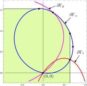
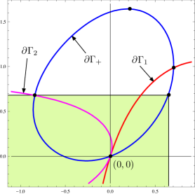
Figure 1: The light-green areas are domains ${\cal D}$ for categories I and II

Theorem 2.1 (Theorem 4.2 of KM 2011 )

Under conditions (i)–(iv), we have, for $k=1,2$,

$$\lim_{n\to\infty}\frac{1}{n}\log P(L_{k}\geq n,L_{3-k}=0)=-\tau_{k},$$ (11)

and, for any directional vector $\vec{c}\geq\vec{0}$,

$$\lim_{n\to\infty}\frac{1}{x}\log P(\langle\vec{c},\vec{L}\rangle\geq x)=-\alpha_{\vec{c}},$$ (12)

where we recall that $\alpha_{\vec{c}}=\sup\{x\geq 0;x\vec{c}\in{\cal D}\}$. Furthermore, if $\gamma(\alpha_{\vec{c}}\vec{c})=1$ and if $\gamma_{k}(\alpha_{\vec{c}}\vec{c})\neq 1$ and $\alpha_{\vec{c}}c_{k}\neq\theta^{(\infty)}_{kk}$ for $k=1,2$, then we have the following exact asymptotics.

$$\lim_{x\to\infty}e^{\alpha_{\vec{c}}x}P(\langle\vec{c},\vec{L}\rangle\geq x)=b_{\vec{c}}.$$ (13)

In this paper, we aim to refine these asymptotics to be exact when $\vec{c}$ is either $(1,0)$, $(0,1)$ or $(1,1)$. Recall that a sequence of nonnegative number $\{p(n);n\in\mathbb{Z}_{+}\}$ is said to have the exact asymptotic $(1+b(-1)^{n})n^{-\kappa}\alpha^{-n}$ for constants $\kappa$ and $\alpha>1$ if there exist real number $b\in[-1,1]$ and a positive constant $c$ such that

$$\lim_{n\to\infty}(1+b(-1)^{n})n^{\kappa}\alpha^{n}p(n)=c.$$ (14)

We note that this asymptotic is equivalent to

$$\lim_{n\to\infty}(1+b(-1)^{n})n^{\kappa}\alpha^{n}\sum_{\ell=n}^{\infty}p(\ell)=c^{\prime}$$ (15)

for some $c^{\prime}>0$. Thus, there is no difference on the exact asymptotic between $P(L_{k}\geq n)$ and $P(L_{k}=n)$. In what follows, we are mainly concerned with the latter type of exact asymptotics.

3 Analytic function method

Our basic idea for deriving exact asymptotics is to adapt the method used in Dai-Miyazawa 2011a which extends the moment generating functions to complex variable analytic functions, and gets the exact tail asymptotics from analytic behavior around their singular points. A similar method is called a kernel method in some literature Guillemin-Leeuwaarden 2011 ; Li-Zhao 2009 ; Li-Zhao 2011a ; Li-Zhao 2011b . We here call it an analytic function method because our approach heavily use the convergence domain ${\cal D}$, which is not the case for the kernel method. See Miyazawa 2011 for more details.

There is one problem in adapting the method of Dai-Miyazawa 2011a because the moment generating functions $\gamma_{k}(\vec{\theta})$ are not polynomials, while the corresponding functions of SRBM are polynomial. If they are not polynomials, the analytic function approach is hard to apply. This problem is resolved if we use generating functions instead of moment generating functions. We here thanks for the skip free assumption.

3.1 Convergence domain of a generating function

Let us convert results on moment generating functions to those on generating function, using a mapping from $\vec{z}\equiv(z_{1},z_{2})\in\mathbb{C}$ to $\vec{g}(\vec{z})\equiv(e^{z_{1}},e^{z_{2}})\in\mathbb{C}$. In particular, for $\vec{\theta}\in\mathbb{R}^{2}$, $\vec{g}(\vec{\theta})\in(\mathbb{R}_{+}^{\rm o})^{2}$, where $\mathbb{R}_{+}^{\rm o}=(0,\infty)$. We use the following notations for $k=1,2$.

$$(u^{(k,\min)}_{1},u^{(k,\min)}_{2})=\vec{g}(\vec{\theta}^{(k,\min)}),\qquad(u^{(k,\max)}_{1},u^{(k,\max)}_{2})=\vec{g}(\vec{\theta}^{(k,\max)}),$$

$$(u^{(k,{\rm r})}_{1},u^{(k,{\rm r})}_{2})=\vec{g}(\vec{\theta}^{(k,{\rm r})}),\hskip 45.20819pt(u^{(k,{\Gamma})}_{1},u^{(k,{\Gamma})}_{2})=\vec{g}(\vec{\theta}^{(k,{\Gamma})}).$$

$$(\tilde{\tau}_{1},\tilde{\tau}_{2})=\vec{g}(\vec{\tau}),$$

We now transfer the results on the moment generating functions in Section 2 to those on the generating functions. For this, we define

$$\tilde{{\cal D}}=\{\vec{g}(\vec{\theta})\in\mathbb{R}_{+}^{2};\vec{\theta}\in{\cal D}\},$$

$$\tilde{\Gamma}_{k}=\{\vec{g}(\vec{\theta})\in\mathbb{R}_{+}^{2};\vec{\theta}\in\Gamma_{k}\},\quad k=1,2,+.$$

Define the following generating functions. For $k=0,1,2,+$,

$$\tilde{\gamma}_{k}(\vec{z})=E(z_{1}^{X^{(k)}_{1}}z_{2}^{X^{(k)}_{2}}),\quad\vec{z}\equiv(z_{1},z_{2})\in\mathbb{C}^{2},$$

which exists except for $z_{1}=0$ or $z_{2}=0$. Similarly,

$$\tilde{\varphi}(\vec{z})=E(z_{1}^{L_{1}}z_{2}^{L_{2}}),$$

$$\tilde{\varphi}_{+}(\vec{z})=E(z_{1}^{L_{1}}z_{2}^{L_{2}}1(\vec{L}\in S_{+})),$$

$$\tilde{\varphi}_{k}(z_{k})=E(z_{k}^{L_{k}}1(\vec{L}\in S_{k})),\qquad k=1,2.$$

as long as they exist.

Obviously, these generating functions are obtained from the corresponding moment generating functions using the inverse mapping $\vec{g}^{-1}$.

$$\tilde{\gamma}_{k}(\vec{z})=\gamma_{k}(\log z_{1},\log z_{2}),\quad k=0,1,2,+,\qquad$$

$$\tilde{\varphi}(\vec{z})=\varphi(\log z_{1},\log z_{2}),$$

$$\tilde{\varphi}_{+}(\vec{z})=\varphi_{+}(\log z_{1},\log z_{2}),$$

$$\tilde{\varphi}_{k}(z)=\varphi_{k}(\log z),\qquad k=1,2,$$

Then, the stationary equation (7) can be written as

$$(1-\tilde{\gamma}_{+}(\vec{z}))\tilde{\varphi}_{+}(\vec{z})+(1-\tilde{\gamma}_{1}(\vec{z}))\tilde{\varphi}_{1}(z_{1})$$ (16)

$$\hskip 43.05542pt+(1-\tilde{\gamma}_{2}(\vec{z}))\tilde{\varphi}_{2}(z_{2})+(1-\tilde{\gamma}_{0}(\vec{z}))\nu(\vec{0})=0.\qquad$$

It is easy to see that

$$\tilde{\Gamma}_{k}\equiv\{\vec{u}\in\mathbb{R}_{+}^{2};\vec{u}>\vec{0},\tilde{\gamma}_{k}(\vec{u})<1\},\quad k=1,2,+,$$

$$\tilde{{\cal D}}\equiv\{\vec{u}\in\mathbb{R}_{+}^{2};\vec{u}>\vec{0},\tilde{\varphi}(\vec{u})<\infty\},$$

It is notable that these sets may not be convex because two dimensional generating functions may not be convex (see Figure 2).

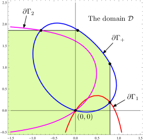
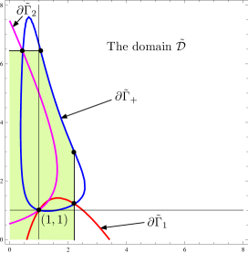
Figure 2: The examples of ${\cal D}$ and the corresponding $\tilde{{\cal D}}$, which may not be convex, where $(p_{21},p_{01},p_{11})=(0.1,0.1,0.7),(p_{20},p_{00},p_{10})=(1.5,0.5,0.5),(p_{22},p_{02},p_{12})=(2,3,1)$ for $p_{ij}=P(\vec{X}^{(+)}=(i,j))$.

Nevertheless, they still have nice properties because the generating functions are polynomials with nonnegative coefficients. To make this specific, we introduce the following terminology.

Definition 1

A subset $A$ of $\mathbb{R}^{2}$ is said to be nonnegative-directed (or coordinate-directed) convex if $\lambda\vec{x}+(1-\lambda)\vec{y}\in A$ for any number $\lambda\in[0,1]$ and any $\vec{x},\vec{y}\in A$ such that $\vec{y}-\vec{x}\geq\vec{0}$ (or $\vec{y}-\vec{x}$ in either one of the coordinate axes, respectively).

We then immediately have the following facts.

Lemma 3

$\tilde{{\cal D}}$ is nonnegative-directed convex, and $\tilde{\Gamma}_{k}$ is coordinate-directed convex for for $k=+,0,1,2$.

Note that (16) is valid for $\vec{z}\in\mathbb{C}^{2}$ satisfying $|\vec{z}|\in\tilde{{\cal D}}$ because $|\tilde{\varphi}(\vec{z})|\leq\tilde{\varphi}(|\vec{z}|)$. Furthermore,

$$\{\vec{z}\in\mathbb{C}^{2};|\vec{z}|\in\tilde{{\cal D}}\}=\{\vec{z}\in\mathbb{C}^{2};E(e^{L_{1}\log|z_{1}|+L_{2}\log|z_{2}|})<\infty\}$$

$$=\{\vec{g}(\log|z_{1}|+i\arg z_{1},\log|z_{2}|+i\arg z_{2});\vec{z}\in\mathbb{C}^{2},(\log|z_{1}|,\log|z_{2}|)\in{\cal D}\}$$

$$=\vec{g}(\{\vec{z}\in\mathbb{C}^{2},(\Re{z_{1}},\Re{z_{2}})\in{\cal D}\}),$$

where $|\vec{z}|=(|z_{1}|,|z_{2}|)$. Hence, the domain ${\cal D}$ is well transferred to $\tilde{{\cal D}}$. We will work on $\tilde{{\cal D}}$ for finding the analytic behaviors of $\tilde{\varphi}_{1}(z)$ and $\tilde{\varphi}_{2}(z)$ around their dominant singular points. This is different from the kernel method, which directly works on the set of complex vectors $\vec{z}$ satisfying $\tilde{\gamma}_{+}(\vec{z})=1$, and applies deeper complex analysis such as analytic extension on a Riemann surface (e.g., see FIM 1999 ). We avoid it using the domain $\tilde{{\cal D}}$.

3.2 A key function for analytic extension

Once the domain $\tilde{{\cal D}}$ is obtained, the next step is to study analytic behaviors of the generating function $\tilde{\varphi}_{k}$ for $k=1,2$. For this, we use a relation between them by letting $\tilde{\gamma}_{+}(\vec{z})-1=0$ in the stationary equation (16), which removes $\tilde{\varphi}_{+}(\vec{z})$. For this, let us consider the solution $u_{2}>0$ of $\tilde{\gamma}_{+}(u_{1},u_{2})=1$ for each fixed $u_{1}>0$. Since this equation is quadratic concerning $u_{2}$ and $\tilde{{\cal D}}\subset(\mathbb{R}^{\rm o})_{+}^{2}$, it has two positive solutions for each $u_{1}$ satisfying

$$u^{(1,\min)}_{1}\leq u_{1}\leq u^{(1,\max)}_{1}.$$

Denote these solutions by $\underline{\zeta}_{2}(u_{1})$ and $\overline{\zeta}_{2}(u_{1})$ such that $\underline{\zeta}_{2}(u_{1})\leq\overline{\zeta}_{2}(u_{1})$. Similarly, $\underline{\zeta}_{1}(u_{2})$ and $\overline{\zeta}_{1}(u_{2})$ are defined for $u_{2}$ satisfying

$$u^{(2,\min)}_{2}\leq u_{2}\leq u^{(2,\max)}_{2}.$$

One can see these facts also applying the mapping $\vec{g}$ to the convex bounded set ${\cal D}$ (see Lemma 3).

We now adapt the arguments in Dai-Miyazawa 2011a . For this, we first examine the function $\underline{\zeta}_{2}$. Let

$$p_{*k}(u)=E(u^{X^{(+)}_{1}}1(X^{(+)}_{2}=k)),$$

$$p_{k*}(u)=E(u^{X^{(+)}_{2}}1(X^{(+)}_{1}=k)),\quad k=0,1,-1.\qquad$$

Then, $\tilde{\gamma}_{+}(u_{1},u_{2})=1$ can be written as

$$u_{2}^{2}p_{*1}(u_{1})-u_{2}(1-p_{*0}(u_{1}))+p_{*-1}(u_{1})=0.$$ (17)

Hence, we have, for $u\in[u^{(1,\min)}_{1},u^{(1,\max)}_{1}]$,

$$\underline{\zeta}_{2}(u)=\frac{1-p_{*0}(u)-\sqrt{D_{2}(u)}}{2p_{*1}(u)},$$ (18)

where

$$D_{2}(u)=(1-p_{*0}(u))^{2}-4p_{*1}(u)p_{*-1}(u)\geq 0.$$

Since $D_{2}(u^{(1,\min)}_{1})=D_{2}(u^{(1,\max)}_{1})=0$ and $u^{2}D_{2}(u)$ is a polynomial with order 4 at most and order 2 at least by condition (i), $u^{2}D_{2}(u)$ can be factorized as

$$u^{2}D_{2}(u)=(u-u^{(1,\min)}_{1})(u^{(1,\max)}_{1}-u)h_{2}(u),$$

where $h_{2}(u)\neq 0$ for $u\in(u^{(1,\min)}_{1},u^{(1,\max)}_{1})$. This fact can be verified by the mapping $\vec{g}$ from $\Gamma_{+}$ to $\tilde{\Gamma}_{+}$.

To get tail asymptotics, we will use analytic functions. So far, we like to analytically extend the function $\underline{\zeta}_{2}$ from the real interval to a sufficiently large region in the complex plane $\mathbb{C}$. For this, we prepare a series of lemmas. We first refer to the following fact.

Lemma 4 (Lemma 2.3.8 of FIM 1999 )

All the solutions of $z^{2}D_{2}(z)=0$ for $z\in\mathbb{C}$ are real numbers.

In the light of the above arguments, this lemma immediately leads to the following fact.

Lemma 5

$z^{2}D_{2}(z)=0$ for $z\in\mathbb{C}$ has no solution in the region such that $|z|\in(u^{(1,\min)}_{1},u^{(1,\max)}_{1})$.

We will also use the following two lemmas, which show how the periodic nature of the random walk $\{\vec{Y}_{\ell}\}$ is related to the branch points (see Remark 2 for the periodic nature). They are proved in Appendices A and B, respectively.

Lemma 6

The equation:

$$D_{2}(z)=0,\qquad|z|=u^{(1,\max)}_{1},\;z\in\mathbb{C},$$ (19)

has only one solution $z=u^{(1,\max)}_{1}$ if and only if (v-a) holds. Otherwise, it has two solutions $z=\pm u^{(1,\max)}_{1}$, and $u^{2}D_{2}(u)$ is an even function.

Lemma 7

For each fixed $x,y>0$, we have

$$\tilde{\gamma}_{+}(x,y)=1,\qquad\tilde{\gamma}_{+}(-x,-y)=1,$$ (20)

if and only if (v-a) does not hold.

Remark 4

Lemma 6 is essentially the same as Remark 3.1 of Li-Zhao 2011b , which is obtained as a corollary of their Lemma 3.1, which is immediate from Lemmas 2.3.8 of FIM 1999 .

By Lemmas 4 and 5, $\underline{\zeta}_{2}(u)$ on $(u^{(1,\min)}_{1},u^{(1,\max)}_{1})$ is extendable as an analytic function of a complex variable to the region $\tilde{{\cal G}}_{0}(u^{(1,\min)}_{1},u^{(1,\max)}_{1})$, where

$$\tilde{{\cal G}}_{0}(a,b)=\{z\in\mathbb{C};z\not\in(-\infty,a]\cup[b,\infty)\},\qquad a,b\in\mathbb{R},$$

and has a single branch point $u^{(1,\max)}_{1}$ on $|z|=u^{(1,\max)}_{1}$ if (v-a) hold, and two branch points $\pm u^{(1,\max)}_{1}$ there otherwise by Lemmas 6 and 5. Both branch points have order two. We denote this extended analytic function by $\underline{\zeta}_{2}(z)$. That is, we use the same notation for an analytically extended function. We identify it by its argument. The following lemma is a key for our arguments. The idea of this lemma is similar to Lemma 6.3 of Dai-Miyazawa 2011a , but its proof is entirely different from that lemma.

Lemma 8

(a) $\underline{\zeta}_{2}$ of (18) is analytically extended on $\tilde{{\cal G}}_{0}(u^{(1,\min)}_{1},u^{(1,\max)}_{1})$.
(b) For $z\in\mathbb{C}\mbox{ satisfying }|z|\in(u^{(1,\min)}_{1},u^{(1,\max)}_{1}]$,

$$|\underline{\zeta}_{2}(z)|\leq\underline{\zeta}_{2}(|z|)\leq u^{(1,\max)}_{2},$$ (21)

where the second inequality is strict if $|z|<u^{(1,\max)}_{1}$.
(c) If either $m^{(1)}_{2}=0$ or (v-b) holds, then

$$\tilde{\gamma}_{1}(z,\underline{\zeta}_{2}(z))=1,\qquad|z|=u^{(1,{\rm r})}_{1},$$ (22)

has no solution other than $z=u^{(1,{\rm r})}_{1}$.
(d) The equation (22) has two solutions $z=\pm u^{(1,{\rm r})}_{1}$ if and only if neither $m^{(1)}_{2}=0$, (v-a) nor (v-b) holds.

Proof

We have already proved (a). Thus, we only need to prove (b), (c) and (d). We first prove (b). For this, it is sufficient to prove (21) for $|z|<u^{(1,\max)}_{1}$ by the continuity of $\underline{\zeta}_{2}(z)$ for $|z|\leq u^{(1,\max)}_{1}$ at $z=u^{(1,\max)}_{1}$. Substituting complex numbers $z_{1}$ and $z_{2}$ into $u_{1}$ and $u_{2}$ of (17), we have

$$z_{2}^{2}p_{*1}(z_{1})+z_{2}p_{*0}(z_{1})+p_{*-1}(z_{1})=z_{2}.$$ (23)

Obviously, this equation has the following solutions for each fixed $z_{1}$ such that $|z_{1}|\in(u^{(1,\min)}_{1},u^{(1,\max)}_{1})$.

$$z_{2}=\underline{\zeta}_{2}(z_{1}),\quad\overline{\zeta}_{2}(z_{1}).$$ (24)

We next take the absolute values of both sides of (23), then

$$|z_{2}|^{2}p_{*1}(|z_{1}|)+|z_{2}|p_{*0}(|z_{1}|)+p_{*-1}(|z_{1}|)\geq|z_{2}|.$$

Thus, we get

$$|z_{2}|(\tilde{\gamma}_{+}(|z_{1}|,|z_{2}|)-1)\geq 0.$$

By the definitions of $\underline{\zeta}_{2}(|z_{1}|)$ and $\overline{\zeta}_{2}(|z_{1}|)$, this inequality can be written as

$$(|z_{2}|-\underline{\zeta}_{2}(|z_{1}|))(|z_{2}|-\overline{\zeta}_{2}(|z_{1}|))=|z_{2}|(\tilde{\gamma}_{+}(|z_{1}|,|z_{2}|)-1)\geq 0.$$

Hence, $\underline{\zeta}_{2}(|z_{1}|)\leq\overline{\zeta}_{2}(|z_{1}|)$ implies

$$|z_{2}|\leq\underline{\zeta}_{2}(|z_{1}|)\quad\mbox{ or }\quad\overline{\zeta}_{2}(|z_{1}|)\leq|z_{2}|.$$ (25)

By (24), we can substitute $z_{2}=\underline{\zeta}_{2}(z_{1})$ into (25), and get

$$|\underline{\zeta}_{2}(z_{1})|\leq\underline{\zeta}_{2}(|z_{1}|)\quad\mbox{or}\quad\overline{\zeta}_{2}(|z_{1}|)\leq|\underline{\zeta}_{2}(z_{1})|,\qquad|z_{1}|\in(u^{(1,\min)}_{1},u^{(1,\max)}_{1}).\quad$$ (26)

Thus, (b) is obtained if we show that $\overline{\zeta}_{2}(|z_{1}|)\leq|\underline{\zeta}_{2}(z_{1})|$ is impossible. Suppose the contrary of this, that is, there is a $z_{1}^{(0)}$ such that

$$\overline{\zeta}_{2}(|z_{1}^{(0)}|)\leq|\underline{\zeta}_{2}(z_{1}^{(0)})|,\qquad|z_{1}^{(0)}|\in(u^{(1,\min)}_{1},u^{(1,\max)}_{1}).$$ (27)

Since $|\underline{\zeta}_{2}(z)|$ is continuous and converges to $\underline{\zeta}_{2}(|z^{(0)}_{1}|)$ as $z$ goes to $|z_{1}^{(0)}|$ on the path that $|z|=|z_{1}^{(0)}|$, there must be a $z_{1}^{(1)}$ such that $|z_{1}^{(1)}|=|z_{1}^{(0)}|$ and

$$\underline{\zeta}_{2}(|z_{1}^{(1)}|)<|\underline{\zeta}_{2}(z_{1}^{(1)})|<\overline{\zeta}_{2}(|z_{1}^{(1)}|)$$

Since $|z_{1}^{(1)}|=|z_{1}^{(0)}|\in(u^{(1,\min)}_{1},u^{(1,\max)}_{1})$, this contradicts (26), which proves (b).

We next prove (c). Let

$$p^{(1)}_{*k}(z)=E(z^{X^{(1)}_{1}}1(X^{(1)}_{2}=k)),\qquad k=0,1.$$

First, assume that $m^{(1)}_{2}=0$. This implies $p^{(1)}_{*1}(z)=0$, and therefore (22) is reduced to $p^{(1)}_{*0}(z)=1$. Hence, its solution is $z=1$ or $z=p^{(1)}_{-10}/p^{(1)}_{10}\geq 0$ if $p^{(1)}_{10}\neq 0$ (otherwise, $z=1$ is only the solution). Both are nonnegative numbers, and therefore (22) has no solution $z$ such that

$$|z|=u^{(1,{\rm r})}_{1},\qquad z\neq u^{(1,{\rm r})}_{1}.$$ (28)

We next assume that $m^{(1)}_{2}\neq 0$, which implies $p^{(1)}_{*1}(z)\neq 0$. Since (22) can be written as

$$\underline{\zeta}_{2}(z)p^{(1)}_{*1}(z)+p^{(1)}_{*0}(z)=1$$ (29)

and $1\leq|w|+|1-w|$ for any $w\in\mathbb{C}$, we have

$$|\underline{\zeta}_{2}(z)|=\left|\frac{1-p^{(1)}_{*0}(z)}{p^{(1)}_{*1}(z)}\right|\geq\frac{1-|p^{(1)}_{*0}(z)|}{|p^{(1)}_{*1}(z)|}\geq\frac{1-p^{(1)}_{*0}(|z|)}{p^{(1)}_{*1}(|z|)}=\underline{\zeta}_{2}(|z|).$$ (30)

If (28) holds, then both sides of this inequality are identical if and only if (v-b) does not hold. Hence, if (v-b) holds, then $|\underline{\zeta}_{2}(z)|>\underline{\zeta}_{2}(|z|)$, and therefore (22) has no solution satisfying (28) because of (21).

We finally prove (d). For this, we assume that both of $m^{(2)}_{1}=0$ and (v-b) do not hold. In this case, $p^{(1)}_{01}=p^{(1)}_{(-1)0}=p^{(1)}_{10}=0$, so it follows from (29) that

$$\underline{\zeta}_{2}(z)=\frac{(1-p^{(1)}_{00})z}{p^{(1)}_{-11}+p^{(1)}_{11}z^{2}}.$$

Hence, if (28) holds, then we must have $z=-u^{(1,{\rm r})}_{1}$ because of (21) and (30). By the above equation, we also have $\underline{\zeta}_{2}(-u^{(1,{\rm r})}_{1})=-\underline{\zeta}_{2}(u^{(1,{\rm r})}_{1})$. Hence, we need to check whether $(-u^{(1,{\rm r})}_{1},-\underline{\zeta}_{2}(u^{(1,{\rm r})}_{1}))$ be the solution of $\gamma_{+}(x,y)=1$. By Lemma 7, $z=-u^{(1,{\rm r})}_{1}$ is the solution of (22) if and only if (v-a) does not hold. Combining this with (b) and (c) completes the proof of (d). ∎

Table 1: The solutions of (19) and (22), where $\bigcirc$, $\times$ and $-$ indicate “yes”, “no” and ‘”irrelevant”.

Non-arithmetic: (v-a)	$\bigcirc$	$\hskip 7.74998pt\times$	$\hskip 7.74998pt\times\hskip 7.74998pt$	$\hskip 7.74998pt\times\hskip 7.74998pt$	$\times$
Non-arithmetic: (v-b)	$-$	$\bigcirc$	$\bigcirc$	$\times$	$\times$
$m^{(1)}_{2}=0$	$-$	$\bigcirc$	$\times$	$\bigcirc$	$\times$
The solutions of (19)	$\hskip 12.91663ptu^{(1,\max)}_{1}\hskip 12.91663pt$	$\pm u^{(1,\max)}_{1}$
The solutions of (22)	$u^{(1,{\rm r})}_{1}$	$u^{(1,{\rm r})}_{1}$			$\pm u^{(1,{\rm r})}_{1}$

For convenience of later reference, we summarize the results in (c) and (d) of Lemma 8 in Table 1. Similar results can be obtained in the direction of the 2nd axes using (v-b) and $m^{(2)}_{1}=0$ instead of (v-a) and $m^{(1)}_{2}=0$. Since the results are symmetric, we omit them. We remark that Li and Zhao Li-Zhao 2011b have not considered the cases $m^{(2)}_{1}=0$ and $m^{(1)}_{2}=0$, which seems to be overlooked.

3.3 Nature of the dominant singularity

We consider complex variable functions $\tilde{\varphi}_{1}(z_{1})$ and $\tilde{\varphi}_{2}(z_{2})$. Recall that

$$\tilde{\varphi}(\vec{z})=\tilde{\varphi}_{+}(\vec{z})+\tilde{\varphi}_{1}(z_{1})+\tilde{\varphi}_{2}(z_{2})+\nu(\vec{0}).$$ (31)

Obviously, $\tilde{\varphi}(\vec{z})$ is analytic for $\vec{z}\in\mathbb{C}^{2}$ such that $(|z_{1}|,|z_{2}|)\in\tilde{{\cal D}}$, and singular on the boundary of $\tilde{{\cal D}}$. This implies that $\tilde{\varphi}_{i}(z_{i})$ is analytic for $|z_{i}|<\tilde{\tau}_{i}$ and has a point on the circle $|z|=\tilde{\tau}_{i}$. This is easily seen from (31) with $z_{j}=0$ for $j=3-i$. Furthermore, $z_{i}=\tilde{\tau}_{i}$ must be a singular point for $i=1,2$ by Pringsheim’s theorem (see, e.g., Theorem 17.13 in Volume 1 of Markushevich Markushevich 1977 ). In addition to this point, we need to find all singular points on $|z|=\tilde{\tau}_{i}$ to get the tail asymptotics as we will see. As expected from Lemma 6, $z=-\tilde{\tau}_{i}$ may be another singular point, which occurs only when (v-a) does not hold.

We focus on these singular points instead of searching singular points on $|z|=\tilde{\tau}_{i}$, and show that there is no other singular point on the circle through analytic behavior of $\tilde{\varphi}_{i}(z)$. Since results are symmetric for $\tilde{\varphi}_{1}(z)$ and $\tilde{\varphi}_{2}(z)$, we only consider $\tilde{\varphi}_{1}(z)$ in this section.

For this, we use the stationary equation (16), which is valid on $\tilde{{\cal D}}$. Plugging $(z_{1},z_{2})=(z,\underline{\zeta}_{2}(z))$ into (16) yields, for $|z|\in(u^{(1,\min)}_{1},\tilde{\tau}_{1})$,

$$\tilde{\varphi}_{1}(z)=\frac{(\tilde{\gamma}_{2}(z,\underline{\zeta}_{2}(z))-1)\tilde{\varphi}_{2}(\underline{\zeta}_{2}(z))}{1-\tilde{\gamma}_{1}(z,\underline{\zeta}_{2}(z))}+\frac{(\tilde{\gamma}_{0}(z,\underline{\zeta}_{2}(z))-1)\nu(\vec{0})}{1-\tilde{\gamma}_{1}(z,\underline{\zeta}_{2}(z))}.$$ (32)

In the light of this equation, the dominant singularity of $\tilde{\varphi}_{1}(z)$ is caused by $\underline{\zeta}_{2}(z)$, $\tilde{\varphi}_{2}(\underline{\zeta}_{2}(z))$ or

$$\tilde{\gamma}_{1}(z,\underline{\zeta}_{2}(z))=1.$$ (33)

In addition to $\tilde{{\cal G}}_{0}(a,b)$, we will use the following sets for considering analytic regions (see Figure 3).

$$\tilde{C}_{\delta}(u)=\{z\in\mathbb{C};u-\delta<|z|<u+\delta,z\neq u\},\qquad u,\delta>0,$$

$$\tilde{{\cal G}}^{+}_{\delta}(u)=\tilde{{\cal G}}_{0}(u^{(1,\min)}_{1},u)\cap\tilde{C}_{\delta}(u),\qquad u^{(1,\min)}_{1}<u,$$

$$\tilde{{\cal G}}^{-}_{\delta}(u)=\tilde{{\cal G}}_{0}(u,-u^{(1,\min)}_{1})\cap\tilde{C}_{\delta}(u),\qquad u<-u^{(1,\min)}_{1}.$$

Remark 5

One may wonder whether (21) in Lemma 8 is sufficient for verifying analyticity of $\tilde{\varphi}_{1}(z)$ in $\tilde{{\cal G}}^{+}_{\delta}(u^{(1,\max)}_{1})$ when $\tilde{\tau}_{1}=u^{(1,\max)}_{1}$. This will turn out to have no problem because of (32).

Figure 3: The shaded area is $\tilde{{\cal G}}^{-}_{\delta}(-u^{(1,\max)}_{1})\cap\tilde{{\cal G}}^{+}_{\delta}(u^{(1,\max)}_{1})$

In what follows, we first consider the case when (v-a) holds, then consider the other case.

Singularity for the non-arithmetic case

Assume the non-arithmetic condition (v-a). We consider the analytic behavior of $\tilde{\varphi}_{1}(z)$ around the singular point $z=\tilde{\tau}_{1}$. This behavior will show that there is no other singular point on $|z|=\tilde{\tau}_{1}$. We separately consider the three causes which are discussed above.

(3a) The solution of (33): This equation has six solutions at most because it can be written as a polynomial equation with order six. $z=1,u^{(1,{\rm r})}_{1}$ are clearly the solutions. Because $\tilde{\varphi}_{1}(z)$ of (32) is analytic for $|z|<\tilde{\tau}_{1}$, (33) can not have solution such that $|z|<\tilde{\tau}_{1}$ except for the points where the numerator of the right hand side of (32) vanishes. This must be finitely many because the numerator vanishes otherwise by the uniqueness of analytic extension. On the other hand, (33) has no solution on the circle $|z|=u^{(1,{\rm r})}_{1}$ except for $z=u^{(1,{\rm r})}_{1}$ by Lemma 8.

Thus, the compactness of the circle implies that, if $\tilde{\tau}_{1}=u^{(1,{\rm r})}_{1}<u^{(1,\max)}_{1}$, then (33) has no solution on $\tilde{C}_{\delta}(u^{(1,{\rm r})}_{1})$ for some $\delta>0$. Hence, we have the following fact from (32).

Lemma 9

Assume that $\tilde{\tau}_{1}=u^{(1,{\rm r})}_{1}<u^{(1,\max)}_{1}$ and $\tilde{\varphi}_{2}(\underline{\zeta}_{2}(z))$ is analytic at $|z|=u^{(1,{\rm r})}_{1}$. Then, $\tilde{\varphi}_{1}(z)$ has a simple pole at $z=u^{(1,{\rm r})}_{1}$, and analytic on $\tilde{C}_{\delta}(u^{(1,{\rm r})}_{1})$.

Remark 6

For categories I and III , the analytic condition on $\tilde{\varphi}_{2}(\underline{\zeta}_{2}(z))$ in this lemma is always satisfied because Lemma 8 and the category condition, $\underline{\zeta}_{2}(\tilde{\tau}_{1})<\tilde{\tau}_{2}$, imply, for $|z|=u^{(1,{\rm r})}_{1}$,

$$|\tilde{\varphi}_{2}(\underline{\zeta}_{2}(z))|\leq\tilde{\varphi}_{2}(|\underline{\zeta}_{2}(z)|)\leq\tilde{\varphi}_{2}(\underline{\zeta}_{2}(|z|))=\tilde{\varphi}_{2}(u^{(1,{\rm r})}_{2})<\infty.$$

If $\tilde{\tau}_{1}=u^{(1,{\rm r})}_{1}=u^{(1,\max)}_{1}$, then the analytic behavior of $\tilde{\varphi}_{1}(z)$ around $z=u^{(1,{\rm r})}_{1}$ is a bit complicated because $\underline{\zeta}_{2}(z)$ is also singular there. We will consider this case in Section 4.

(3b) The singularity of $\underline{\zeta}_{2}(z)$: By Lemma 8, this function is analytic on $\tilde{{\cal G}}_{0}(u^{(1,\min)}_{1},u^{(1,\max)}_{1})$ and singular at $z=u^{(1,\max)}_{1}$, which is a branch point.

(3c) The singularity of $\tilde{\varphi}_{2}(\underline{\zeta}_{2}(z))$: This function is singular at $z=\tilde{\tau}_{1}$ if $\underline{\zeta}_{2}(\tilde{\tau}_{1})=\tilde{\tau}_{2}$. Otherwise, it is singular at $z=u^{(1,\max)}_{1}$ because $\underline{\zeta}_{2}(z)$ is singular there. Furthermore, we may simultaneously have $\underline{\zeta}_{2}(\tilde{\tau}_{1})=\tilde{\tau}_{2}$ and $\tilde{\tau}_{1}=u^{(1,\max)}_{1}$. Thus, we need to consider these three cases: $\tilde{\tau}_{1}=u^{(1,\max)}_{1}$ for categories I and III , and $\tilde{\tau}_{1}<u^{(1,\max)}_{1}$ or $\tilde{\tau}_{1}=u^{(1,\max)}_{1}$ for category II . For this, we will use the following fact, which is essentially the same as Lemma 4.2 of MR 2009 .

Lemma 10

$\overline{\zeta}_{1}(e^{\theta})$ is a concave function of $\theta\in[\theta^{(2,\min)}_{2},\theta^{(2,\max)}_{2}]$, $\overline{\zeta}_{1}^{\prime}(u^{(1,\max)}_{2})=0$, $\overline{\zeta}_{1}^{\prime\prime}(u^{(1,\max)}_{2})<0$, and

$$\lim_{z\to u^{(1,\max)}_{1}\atop z\in\tilde{{\cal G}}_{0}(u^{(1,\min)}_{1},u^{(1,\max)}_{1})}\frac{u^{(1,\max)}_{2}-\underline{\zeta}_{2}(z)}{(u^{(1,\max)}_{1}-z)^{\frac{1}{2}}}=\frac{\sqrt{2}}{\sqrt{-\overline{\zeta}_{1}^{\prime\prime}(u^{(1,\max)}_{2})}}.$$ (34)

Proof

The first part is immediate from the facts that $\Gamma_{+}$ is a convex set and $u^{(1,\max)}_{1}=e^{\theta^{(1,\max)}_{1}}$. By Taylor expansion of $\overline{\zeta}_{1}(z_{2})$ at $z_{2}=u^{(1,\max)}_{2}<u^{(2,\max)}_{2}$,

$$\overline{\zeta}_{1}(z_{2})=u^{(1,\max)}_{1}+\frac{1}{2}\overline{\zeta}_{1}^{\prime\prime}(u^{(1,\max)}_{2})(z_{2}-u^{(1,\max)}_{2})^{2}+o(|z_{2}-u^{(1,\max)}_{2}|^{2}).$$

Letting $z_{2}=\underline{\zeta}_{2}(z)$ in this equation yields (34) since $\overline{\zeta}_{1}(\underline{\zeta}_{2}(z))=z$ for $z$ to be sufficiently close to $u^{(1,\max)}_{1}$. ∎

Another useful asymptotic is:

Lemma 11

If $u^{(1,\max)}_{1}=u^{(1,{\rm r})}_{1}$, then for any $\delta>0$,

$$\lim_{z\to u^{(1,\max)}_{1}\atop z\in\tilde{{\cal G}}^{+}_{\delta}(u^{(1,\max)}_{1})}\frac{(u^{(1,\max)}_{1}-z)^{\frac{1}{2}}}{1-\tilde{\gamma}_{1}(z,\underline{\zeta}_{2}(z))}=\frac{\sqrt{-\overline{\zeta}_{1}^{\prime\prime}(u^{(1,\max)}_{2})}}{\sqrt{2}p^{(1)}_{*1}(u^{(1,{\rm r})}_{1})}.$$ (35)

Proof

By the condition $u^{(1,\max)}_{1}=u^{(1,{\rm r})}_{1}$, we have

$$1-\tilde{\gamma}_{1}(z,\underline{\zeta}_{2}(z))=\tilde{\gamma}_{1}(\vec{u}^{(1,\max)})-\tilde{\gamma}_{1}(z,\underline{\zeta}_{2}(z))$$

$$=(u^{(1,\max)}_{2}-\underline{\zeta}_{2}(z))p^{(1)}_{*1}(u^{(1,{\rm r})}_{1})$$

$$\qquad+\underline{\zeta}_{2}(z)(p^{(1)}_{*1}(u^{(1,{\rm r})}_{1})-p^{(1)}_{*1}(z))+p^{(1)}_{*0}(u^{(1,{\rm r})}_{1})-p^{(1)}_{*0}(z).$$

Hence, by dividing both sides by $(u^{(1,\max)}_{1}-z)^{\frac{1}{2}}$, Lemma 10 yields (34) because $p^{(1)}_{*1}(z)$ and $p^{(1)}_{*0}(z)$ are analytic except for $z=0$. ∎

We now consider the three cases separately.

(3c-1) $\underline{\zeta}_{2}(\tilde{\tau}_{1})<\tilde{\tau}_{2}$, equivalently, categories I or III , and $\tilde{\tau}_{1}=u^{(1,\max)}_{1}$: In this case, $\tilde{\varphi}_{2}(z)$ is analytic for $z\in\tilde{C}_{\delta}(u^{(1,\max)}_{2})$ for some $\delta>0$ because $u^{(1,\max)}_{2}=\underline{\zeta}_{2}(u^{(1,\max)}_{1})=\underline{\zeta}_{2}(\tilde{\tau}_{1})<\tilde{\tau}_{2}$. Hence, by Taylor expansion, we have, for $|z|<\tilde{\tau}_{2}$,

$$\tilde{\varphi}_{2}(z)=\tilde{\varphi}_{2}(u^{(1,\max)}_{2})+\tilde{\varphi}_{2}^{\prime}(u^{(1,\max)}_{2})(z-u^{(1,\max)}_{2})+o(|z-u^{(1,\max)}_{2}|).$$ (36)

Thus the analytic behavior of $\tilde{\varphi}_{2}(\underline{\zeta}_{2}(z))$ around $z=u^{(1,\max)}_{1}$ is determined by that of $\underline{\zeta}_{2}(z)-u^{(1,\max)}_{2}$. Since $u^{(1,\max)}_{2}=\underline{\zeta}_{2}(u^{(1,\max)}_{1})<\tilde{\tau}_{2}$ by the conditions of (3c-1), Lemma 10 yields

$$\tilde{\varphi}_{2}(\underline{\zeta}_{2}(z))=\tilde{\varphi}_{2}(u^{(1,\max)}_{2})-\frac{\sqrt{2}\tilde{\varphi}_{2}^{\prime}(u^{(1,\max)}_{2})}{\sqrt{-\overline{\zeta}_{1}^{\prime\prime}(u^{(1,\max)}_{2})}}(u^{(1,\max)}_{1}-z)^{\frac{1}{2}}$$ (37)

$$+o(|z-u^{(1,\max)}_{2}|^{\frac{1}{2}}).$$

Thus, $\tilde{\varphi}_{2}(\underline{\zeta}_{2}(z))$ has a branch point of order 2 at $z=\tilde{\tau}_{1}=u^{(1,\max)}_{1}$, and is analytic on $\tilde{{\cal G}}^{+}_{\delta}(u^{(1,\max)}_{1})$ for some $\delta>0$.

(3c-2) $\underline{\zeta}_{2}(\tilde{\tau}_{1})=\tilde{\tau}_{2}$ and $\tilde{\tau}_{1}<u^{(1,\max)}_{1}$: This is only for category II . Hence, $\tilde{\tau}_{2}=u^{(2,{\rm r})}_{2}<u^{(2,\max)}_{2}$, and therefore $\tilde{\varphi}_{2}$-version of Lemma 9 is available. Thus, $\tilde{\varphi}_{2}(z)$ has a simple pole at $z=u^{(2,{\rm r})}_{2}$. Here, $u^{(2,{\rm r})}_{2}$ is the solution of the equation:

$$\tilde{\gamma}_{2}(\underline{\zeta}_{1}(z),z)=1$$ (38)

is crucial. Furthermore, $\underline{\zeta}_{2}(z)$ is analytic at $z=\tilde{\tau}_{1}$. Hence, $\tilde{\varphi}_{2}(\underline{\zeta}_{2}(z))$ has a simple pole at $z=\tilde{\tau}_{1}$, and is analytic on $\tilde{C}_{\delta}(u^{(1,\max)}_{1})$ for some $\delta>0$.

(3c-3) $\underline{\zeta}_{2}(\tilde{\tau}_{1})=\tilde{\tau}_{2}$, and $\tilde{\tau}_{1}=u^{(1,\max)}_{1}$: This is also only for category II . This case is similar to (3c-2) except that $\underline{\zeta}_{2}(z)$ has a branch point at $z=\tilde{\tau}_{1}=u^{(1,\max)}_{1}$. Since $\tilde{\varphi}_{2}(z)$ has a simple pole at $z=\tilde{\tau}_{2}$, we have, by Lemma 10,

$$\tilde{\varphi}_{2}(\underline{\zeta}_{2}(z))\sim(u^{(1,\max)}_{1}-z)^{-\frac{1}{2}},$$

and $\tilde{\varphi}_{2}(\underline{\zeta}_{2}(z))$ is analytic on $\tilde{{\cal G}}^{+}_{\delta}(u^{(1,\max)}_{1})$ for some $\delta>0$.

Singularity for the arithmetic case

We next consider the case that (v-a) does not holds. That is, the Markov additive process for the interior is arithmetic. In this case, the singularity of $\tilde{\varphi}_{1}(z)$ at $z=\tilde{\tau}_{1}$ occurs similarly to in Section 3.3. In addition to this singular point, we may have another singular point $-\tilde{\tau}_{1}$ as can be seen in Table 1. For this, we separately consider two sub-cases:

• either (v-b) or $m^{(1)}_{2}=0$ holds.      (B2)   neither (v-b) nor $m^{(1)}_{2}=0$ holds.

In some cases, we need further classification:

• either (v-c) or $m^{(2)}_{1}=0$ holds.      (C2)   neither (v-b) nor $m^{(2)}_{1}=0$ holds.

Consider (B1). From Table 1, the solutions of (19) are $z=\pm u^{(1,\max)}_{1}$, and the solution of (22) is $z=u^{(1,{\rm r})}_{1}$. There is no other solution. We consider cases similar to (3a), (3b), (3c-2), (3c-1) and (3c-3) of Section 3.3.

• The solution of (33): This case is exactly the same as in Section 3.3 because $z=-u^{(1,{\rm r})}_{1}$ is not the solution of (22). Hence, Lemma 9 also holds true.

• The singularity of $\underline{\zeta}_{2}(z)$ at $|z|=u^{(1,\max)}_{1}$: It is singular at $z=\pm u^{(1,\max)}_{1}$.

• The singularity of $\tilde{\varphi}_{2}(\underline{\zeta}_{2}(z))$ at $|z|=\tilde{\tau}_{1}$: For $z=\tilde{\tau}_{1}$, the story is the same as in Section 3.3. Hence, we only consider the case that $z=-\tilde{\tau}_{1}$. From (18) and the condition that (v-a) does not hold, we have

  $$\underline{\zeta}_{2}(-\tilde{\tau}_{1})=-\frac{1-p_{00}}{2(p_{-11}+p_{11}\tilde{\tau}_{1}^{2})}\tilde{\tau}_{1}=-\underline{\zeta}_{2}(\tilde{\tau}_{1}),$$ (39)

  Hence, $|\underline{\zeta}_{2}(-\tilde{\tau}_{1})|=\underline{\zeta}_{2}(\tilde{\tau}_{1})>0$, and

  $$|\underline{\zeta}_{1}(\underline{\zeta}_{2}(-\tilde{\tau}_{1}))|=|\underline{\zeta}_{1}(-\underline{\zeta}_{2}(\tilde{\tau}_{1}))|=\underline{\zeta}_{1}(\underline{\zeta}_{2}(\tilde{\tau}_{1})).$$

  Since $\underline{\zeta}_{1}(\underline{\zeta}_{2}(\tilde{\tau}_{1}))<\tilde{\tau}_{1}$, $\tilde{\varphi}_{1}(\underline{\zeta}_{1}(\underline{\zeta}_{2}(z)))$ is analytic around $z=-\tilde{\tau}_{1}$. Furthermore, Lemma 10 and (37) are still valid if we replace $u^{(1,\max)}_{i}$ by $-u^{(1,\max)}_{i}$ for $i=1,2$. However, this $z=-\tilde{\tau}_{1}$ can not be the solution of (33) because of (B1). Thus, we have to partially change the arguments in Section 3.3.

  • $\underline{\zeta}_{2}(\tilde{\tau}_{1})<\tilde{\tau}_{2}$ and $\tilde{\tau}_{1}=u^{(1,\max)}_{1}$: This is only for categories I and III , and $\tilde{\varphi}_{2}(\underline{\zeta}_{2}(z))$ has a branch point of order 2 at $z=-u^{(1,\max)}_{1}$, and is analytic on $\tilde{{\cal G}}^{-}_{\delta}(-u^{(1,\max)}_{1})\cap\tilde{{\cal G}}^{+}_{\delta}(u^{(1,\max)}_{1})$ for some $\delta>0$ because it has also a branch point at $z=u^{(1,\max)}_{1}$.

  • $\underline{\zeta}_{2}(\tilde{\tau}_{1})=\tilde{\tau}_{2}$ and $\tilde{\tau}_{1}<u^{(1,\max)}_{1}$: This is only for category II . Since $\underline{\zeta}_{2}(z)$ is analytic at $z=\tilde{\tau}_{1}$, $\tilde{\varphi}_{2}(\underline{\zeta}_{2}(z))$ is analytic at $z=-\tilde{\tau}_{1}$ if (C1) holds. Otherwise, if (C2) holds, it has a simple pole at $z=-\tilde{\tau}_{1}$ because $\underline{\zeta}_{2}(-\tilde{\tau}_{1})=-\underline{\zeta}_{2}(\tilde{\tau}_{1})$ is the solution of (38).

  • $\underline{\zeta}_{2}(\tilde{\tau}_{1})=\tilde{\tau}_{2}$ and $\tilde{\tau}_{1}=u^{(1,\max)}_{1}$: This is only for category II , and the situation is similar to (3c’-2) except that the singularity is caused by $\underline{\zeta}_{2}(z)$ at $z=-\tilde{\tau}_{1}$. To verify this fact, we rework on $\tilde{\varphi}_{2}(\underline{\zeta}_{2}(z))$. Similarly to (32), we have, for $|z|\in(u^{2,\min)}_{2},\tilde{\tau}_{2})$,

    $$\tilde{\varphi}_{2}(z)=\frac{(\tilde{\gamma}_{1}(\underline{\zeta}_{1}(z),z)-1)\tilde{\varphi}_{1}(\underline{\zeta}_{1}(z))}{1-\tilde{\gamma}_{2}(\underline{\zeta}_{1}(z),z)}+\frac{(\tilde{\gamma}_{0}(\underline{\zeta}_{2}(z),z)-1)\nu(\vec{0})}{1-\tilde{\gamma}_{2}(\underline{\zeta}_{1}(z),z)}.$$

    Substituting $\underline{\zeta}_{2}(z)$ into $z$ of this equation, we have

    $$\tilde{\varphi}_{2}(\underline{\zeta}_{2}(z))=\frac{(\tilde{\gamma}_{1}(\underline{\zeta}_{1}(\underline{\zeta}_{2}(z)),\underline{\zeta}_{2}(z))-1)\tilde{\varphi}_{1}(\underline{\zeta}_{1}(\underline{\zeta}_{2}(z)))}{1-\tilde{\gamma}_{2}(\underline{\zeta}_{1}(\underline{\zeta}_{2}(z)),\underline{\zeta}_{2}(z))}$$ (40)

    $$\hskip 43.05542pt+\frac{(\tilde{\gamma}_{0}(\underline{\zeta}_{2}(\underline{\zeta}_{2}(z)),\underline{\zeta}_{2}(z))-1)\nu(\vec{0})}{1-\tilde{\gamma}_{2}(\underline{\zeta}_{1}(\underline{\zeta}_{2}(z)),\underline{\zeta}_{2}(z))}.$$

    By the assumptions of (3c-3), if (C2) holds, then $\tilde{\varphi}_{2}(z)$ has a simple pole at $z=-\tilde{\tau}_{2}$, and therefore $\tilde{\varphi}_{2}(\underline{\zeta}_{2}(z))\sim(-u^{(1,\max)}_{1}-z)^{-\frac{1}{2}}$ around $z=-u^{(1,\max)}_{1}$ by Lemma 10. Otherwise, if (C1) holds, we need to consider $\tilde{\varphi}_{1}(\underline{\zeta}_{1}(\underline{\zeta}_{2}(z)))$ in (40) due to the singularity of $\underline{\zeta}_{2}(z)$ at $z=-\tilde{\tau}_{1}=-u^{(1,\max)}_{1}$, where $\tilde{\varphi}_{1}(\underline{\zeta}_{1}(z))$ is analytic at $z=-u^{(1,\max)}_{2}=-\underline{\zeta}_{2}(u^{(1,\max)}_{1})$ because

    $$|\underline{\zeta}_{1}(\underline{\zeta}_{2}(-\tilde{\tau}_{1}))|=|\underline{\zeta}_{1}(\underline{\zeta}_{2}(\tilde{\tau}_{1}))|<\tilde{\tau}_{1}.$$

    Hence, $\tilde{\varphi}_{1}(\underline{\zeta}_{1}(\underline{\zeta}_{2}(z)))-\tilde{\varphi}_{1}(-\underline{\zeta}_{1}(u^{(1,\max)}_{2}))\sim(-u^{(1,\max)}_{1}-z)^{\frac{1}{2}}$. On the other hand, $\tilde{\gamma}_{1}(\underline{\zeta}_{1}(\underline{\zeta}_{2}(z)),\underline{\zeta}_{2}(z))-1\sim(-u^{(1,\max)}_{1}-z)^{\frac{1}{2}}$ because (v-a) does not hold. Combining these asymptotics in (40), we have $\tilde{\varphi}_{2}(\underline{\zeta}_{2}(z))-\tilde{\varphi}_{2}(-\tilde{\tau}_{2})\sim(-u^{(1,\max)}_{1}-z)^{\frac{1}{2}}$ around $z=-u^{(1,\max)}_{1}$ by Lemma 10.

We next consider (B2). From Table 1, the solutions of (19) are $z=\pm u^{(1,\max)}_{1}$, and the solutions of (22) are $z=\pm u^{(1,{\rm r})}_{1}$. In this case, the arguments for $z=-\tilde{\tau}_{1}$ is completely parallel to those for $z=\tilde{\tau}_{1}$ except for the cases (3c’-2) and (3c’-3). The latter two cases are also parallel if (C2) holds. Otherwise, $\tilde{\varphi}_{2}(z)$ is analytic at $z=-\tilde{\tau}_{2}$.

3.4 Asymptotic inversion formula

From these singularities, we derive exact tail asymptotics of the stationary distribution. For this, we use Tauberian type theorem for generating functions.

Lemma 12 (Theorem VI.5 of Flajolet-Sedqewick 2009 )

Let $f$ be a generating function of a sequence of real numbers $\{p(n);n=0,1,\ldots\}$. If $f(z)$ is singular at finitely many points $a_{1},a_{2},\ldots,a_{m}$ on the circle $|z|=\rho$ for some $\rho>0$ and positive integer $m$, and analytic on the set

$$\Delta_{i}\equiv\{z\in\mathbb{C};|z|<r_{i},z\neq a_{i},|\arg(z-a_{i})|>\omega_{i}\},\quad i=1,2,\ldots,m,$$

for some $\omega_{i}$ and $r_{i}$ such that $\rho<r_{i}$ and $0\leq\omega_{i}<\frac{\pi}{2}$ and if

$$\lim_{\Delta_{i}\ni z\to a_{i}}(a_{i}-z)^{\kappa_{i}}f(z)=b_{i},\qquad i=1,2,\ldots,m,$$ (41)

for $\kappa_{i}\not\in\{0,-1,-2,\ldots\}$ and some constant $b_{i}\in\mathbb{R}$, then

$$\lim_{n\to\infty}\left(\sum_{i=1}^{m}\frac{n^{\kappa_{i}-1}}{\Gamma(\kappa_{i})}a_{i}^{-n}\right)^{-1}p(n)=b,$$ (42)

for some real number $b$, where $\Gamma(z)$ is the gamma function for complex number $z$ (see Sec 52 of Volume II of Markushevich 1977 ).

Recall that the asymptotic notation “$\sim$” introduced in Section 1. With this notation, (42) can be written as

$$p(n)\sim\sum_{i=1}^{m}\frac{n^{\kappa_{i}-1}}{\Gamma(\kappa_{i})}a_{i}^{-n},$$

where $\Gamma(\frac{1}{2})=\sqrt{\pi}$ and $\Gamma(-\frac{1}{2})=-2\sqrt{\pi}$.

We will apply Lemma 12 in the following cases: For $m=1$, $a_{1}=u^{(1,{\rm r})}_{1}$ and $\kappa_{1}=1,2$, $a_{1}=u^{(1,\max)}_{1}$ and $\kappa_{1}=\pm\frac{1}{2}$. For $m=2$, $a_{1}=\pm u^{(1,{\rm r})}_{1}$ and $\kappa_{1}=1,2$, $a_{1}=\pm u^{(1,\max)}_{1}$ and $\kappa_{1}=-\frac{1}{2}$.

4 Exact tail asymptotics for the non-arithmetic case

Throughout this section, we assume the non-arithmetic condition (v-a). We first derive exact asymptotics for the stationary probabilities $\nu(n,0)$ and $\nu(0,n)$ on the boundary faces. Because of symmetry, we are only concerned with $\nu(n,0)$.

4.1 The boundary probabilities for the non-arithmetic case

We separately consider the two cases that $u^{(1,{\Gamma})}_{2}<u^{(2,{\Gamma})}_{2}$ and $u^{(1,{\Gamma})}_{2}\geq u^{(2,{\Gamma})}_{2}$, which correspond with categories I (or III ) and II , respectively. In this subsection, we prove the following two theorems.

Theorem 4.1

Under the conditions (i)–(iv) and (v-a), for categories I and III , $\tilde{\tau}_{1}=u^{(1,{\Gamma})}_{1}$, and $P(L_{1}=n,L_{2}=0)$ has the following exact asymptotic $h_{1}(n)$.

$$h_{1}(n)=\left\{\begin{array}[]{ll}\tilde{\tau}_{1}^{-n},&u^{(1,{\Gamma})}_{1}\not=u^{(1,\max)}_{1},\\ n^{-\frac{1}{2}}\tilde{\tau}_{1}^{-n},&u^{(1,{\Gamma})}_{1}=u^{(1,\max)}_{1}=u^{(1,{\rm r})}_{1},\\ n^{-\frac{3}{2}}\tilde{\tau}_{1}^{-n},&u^{(1,{\Gamma})}_{1}=u^{(1,\max)}_{1}\neq u^{(1,{\rm r})}_{1}.\end{array}\right.$$ (46)

By symmetry, the corresponding results are also obtained for $P(L_{1}=0,L_{2}=n)$ for categories I and II .

Theorem 4.2

Under the conditions (i)–(iv) and (v-a), for category II , $\tilde{\tau}_{2}=u^{(2,{\rm r})}_{2}$, and $P(L_{1}=n,L_{2}=0)$ has the following exact asymptotic $h_{1}(n)$.

$$h_{1}(n)=\left\{\begin{array}[]{ll}\tilde{\tau}_{1}^{-n},&\tilde{\tau}_{1}<u^{(1,{\Gamma})}_{1},\mbox{ or }\\ &\tilde{\tau}_{1}=u^{(1,{\Gamma})}_{1}=u^{(1,\max)}_{1}=u^{(1,{\rm r})}_{1},\\ n\tilde{\tau}_{1}^{-n},&\tilde{\tau}_{1}=u^{(1,{\Gamma})}_{1}\not=u^{(1,\max)}_{1},\\ n^{-\frac{1}{2}}\tilde{\tau}_{1}^{-n},&\tilde{\tau}_{1}=u^{(1,{\Gamma})}_{1}=u^{(1,\max)}_{1}\neq u^{(1,{\rm r})}_{1}.\end{array}\right.$$ (51)

By symmetry, the corresponding results are also obtained for $P(L_{1}=0,L_{2}=n)$ for categories III .

Remark 7

Theorems 4.1 and 4.2 are exactly corresponds with Theorem 6.1 of Dai-Miyazawa 2011b (see also Theorems 2.1 and 2.3 of Dai-Miyazawa 2011a ). This is not surprising because of the similarity of the stationary equations although moment generating functions are used in Dai-Miyazawa 2011a ; Dai-Miyazawa 2011b .

Remark 8

These theorems fill missing cases for the exact asymptotics of Theorem 4.2 of Miyazawa 2009 . Furthermore, they correct two errors there. Both of them are for category II . The exact asymptotic is geometric for $\tilde{\tau}_{1}=u^{(1,{\Gamma})}_{1}=u^{(1,\max)}_{1}=u^{(1,{\rm r})}_{1}$, and not geometric for $\tilde{\tau}_{1}=u^{(1,{\Gamma})}_{1}\not=u^{(1,\max)}_{1}$ (see Theorem 4.2). However, in Theorem 4.2 of Miyazawa 2009 , they are not geometric (see (43d3) there) and geometric (see (4c) there), respectively. Thus, these should be corrected.

Proof of Theorem 4.1. We assume that either in category I or III occurs. This is equivalent to $u^{(1,{\Gamma})}_{2}<u^{(2,{\Gamma})}_{2}$, and $\tilde{\tau}_{1}=u^{(1,{\Gamma})}_{1}$. Furthermore, we always have $\underline{\zeta}_{2}(u^{(1,{\Gamma})}_{1})=u^{(1,{\Gamma})}_{2}<\tilde{\tau}_{2}$, and therefore $\tilde{\varphi}_{2}(\underline{\zeta}_{2}(z))$ is analytic at $z=u^{(1,{\Gamma})}_{1}$. We consider three cases separately.

(4a) $u^{(1,{\Gamma})}_{1}<u^{(1,\max)}_{1}$: This case implies that $u^{(1,{\rm r})}_{1}<u^{(1,\max)}_{1}$ and $\tilde{\gamma}_{1}(\vec{u}^{(1,\max)})>1$, and therefore $\vec{u}^{(1,{\rm r})}=\vec{u}^{(1,{\Gamma})}$. Hence, by Lemma 9, $\tilde{\varphi}_{1}$ of (32) satisfies the conditions of Lemma 12 under the setting (41) with $a_{1}=u^{(1,{\rm r})}_{1}$, $\kappa=1$. Thus, letting

$$b=\frac{(\tilde{\gamma}_{2}(\vec{u}^{(1,{\rm r})})-1)\tilde{\varphi}_{2}(u^{(1,{\rm r})}_{2})+(\tilde{\gamma}_{0}(\vec{u}^{(1,{\rm r})})-1)\nu(\vec{0})}{\frac{d}{du}\tilde{\gamma}_{1}(u,\underline{\zeta}_{2}(u))|_{u=u^{(1,{\rm r})}_{1}}},$$

which must be positive by (42) and the fact that $\tilde{\varphi}_{1}(z)$ is singular at $z=u^{(1,{\rm r})}_{1}$, we have

$$\lim_{n\to\infty}\tilde{\tau}_{1}^{n}P(L_{1}=n,L_{2}=0)=b.$$

(4b) $u^{(1,{\Gamma})}_{1}=u^{(1,\max)}_{1}$, $u^{(1,{\rm r})}_{1}=u^{(1,\max)}_{1}$: In this case, category III is impossible, and $\tilde{\gamma}_{1}(\vec{u}^{(1,\max)})=1$. On the other hand, $\tilde{\varphi}_{2}(z)$ is analytic at $z=\underline{\zeta}_{2}(u^{(1,\max)}_{1})<\tilde{\tau}_{2}$ because of Category I. Hence, we can use the Taylor expansion (36), and therefore (32), (37) and Lemma 11 yield, for some $\delta>0$,

$$\lim_{\tilde{{\cal G}}^{+}_{\delta}(u^{(1,\max)}_{1})\ni z\to u^{(1,\max)}_{1}}(u^{(1,\max)}_{1}-z)^{\frac{1}{2}}\tilde{\varphi}_{1}(z)=b,$$ (52)

where

$$b=\Big{(}(\tilde{\gamma}_{2}(\vec{u}^{(1,\max)})-1)\tilde{\varphi}_{2}(u^{(1,\max)}_{2})+(\tilde{\gamma}_{0}(\vec{u}^{(1,\max)})-1)\nu(\vec{0})\Big{)}\frac{\sqrt{-\overline{\zeta}_{1}^{\prime\prime}(u^{(1,\max)}_{2})}}{\sqrt{2}p^{(1)}_{*1}(u^{(1,{\rm r})}_{1})}.$$

Hence, $\tilde{\varphi}_{1}$ satisfies the conditions of Lemma 12 under the setting (41) with $a_{1}=u^{(1,\max)}_{1}$ and $\kappa_{1}=\frac{1}{2}$, and therefore we have

$$\lim_{n\to\infty}n^{\frac{1}{2}}\tilde{\tau}_{1}^{n}P(L_{1}=n,L_{2}=0)=\frac{b}{\sqrt{\pi}},$$

where the positivity of $b$ is checked similarly to case (4a) (see also case (4c) below).

(4c) $u^{(1,{\Gamma})}_{1}=u^{(1,\max)}_{1}$, $u^{(1,{\rm r})}_{1}\not=u^{(1,\max)}_{1}$: In this case, category III is also impossible, and $\tilde{\gamma}_{1}(\vec{u}^{(1,\max)})\not=1$. Thus, we consider the setting (41) with $\kappa_{1}=-\frac{1}{2}$. From (32), we have

$$\tilde{\varphi}_{1}(z)-\tilde{\varphi}_{1}(u^{(1,\max)}_{1})$$ (53)

$$=\frac{(\tilde{\gamma}_{2}(z,\underline{\zeta}_{2}(z))-1)\tilde{\varphi}_{2}(\underline{\zeta}_{2}(z))+(\tilde{\gamma}_{0}(z,\underline{\zeta}_{2}(z))-1)\nu(\vec{0})}{1-\tilde{\gamma}_{1}(z,\underline{\zeta}_{2}(z))}-\tilde{\varphi}_{1}(u^{(1,\max)}_{1})$$

$$=\frac{(\tilde{\gamma}_{2}(z,\underline{\zeta}_{2}(z))-1)(\tilde{\varphi}_{2}(\underline{\zeta}_{2}(z))-\tilde{\varphi}_{2}(u^{(1,\max)}_{2}))}{1-\tilde{\gamma}_{1}(z,\underline{\zeta}_{2}(z))}$$

$$\quad+\frac{(\tilde{\gamma}_{2}(z,\underline{\zeta}_{2}(z))-\tilde{\gamma}_{2}(\vec{u}^{(1,\max)}))\tilde{\varphi}_{2}(u^{(1,\max)}_{2})}{1-\tilde{\gamma}_{1}(z,\underline{\zeta}_{2}(z))}+\frac{(\tilde{\gamma}_{0}(z,\underline{\zeta}_{2}(z))-\tilde{\gamma}_{0}(\vec{u}^{(1,\max)}))\nu(\vec{0})}{1-\tilde{\gamma}_{1}(z,\underline{\zeta}_{2}(z))}$$

$$\quad+\Bigg{[}\frac{(\tilde{\gamma}_{2}(\vec{u}^{(1,\max)})-1)\tilde{\varphi}_{2}(u^{(1,\max)}_{2})}{(1-\tilde{\gamma}_{1}(z,\underline{\zeta}_{2}(z)))(1-\tilde{\gamma}_{1}(\vec{u}^{(1,\max)}))}+\frac{(\tilde{\gamma}_{0}(\vec{u}^{(1,\max)})-1)\nu(\vec{0})}{(1-\tilde{\gamma}_{1}(z,\underline{\zeta}_{2}(z)))(1-\tilde{\gamma}_{1}(\vec{u}^{(1,\max)}))}\Bigg{]}$$

$$\hskip 21.52771pt\times\left(\tilde{\gamma}_{1}(z,\underline{\zeta}_{2}(z))-\tilde{\gamma}_{1}(\vec{u}^{(1,\max)})\right).$$

We recall (37) that

$$\tilde{\varphi}_{2}(\underline{\zeta}_{2}(z))-\tilde{\varphi}_{2}(u^{(1,\max)}_{2})=-(u^{(1,\max)}_{1}-z)^{\frac{1}{2}}\frac{\sqrt{2}\tilde{\varphi}_{2}^{\prime}(u^{(1,\max)}_{2})}{\sqrt{-\overline{\zeta}_{1}^{\prime\prime}(u^{(1,\max)}_{2})}}+o(|u^{(1,\max)}_{1}-z|^{\frac{1}{2}}).$$

From (34), we have

$$\tilde{\gamma}_{0}(z,\underline{\zeta}_{2}(z))-\tilde{\gamma}_{0}(\vec{u}^{(1,\max)})=(\underline{\zeta}_{2}(z)-\underline{\zeta}_{2}(u^{(1,\max)}_{1}))p^{(0)}_{*1}(z)$$

$$\quad+\underline{\zeta}_{2}(u^{(1,\max)}_{1})(p^{(0)}_{*1}(z)-p^{(0)}_{*1}(u^{(1,\max)}_{1}))+p^{(0)}_{*0}(z)-p^{(0)}_{*0}(u^{(1,\max)}_{1})$$

$$=-\frac{\sqrt{2}p^{(0)}_{*1}(u^{(1,\max)}_{1})}{\sqrt{-\overline{\zeta}_{1}^{\prime\prime}(u^{(1,\max)}_{2})}}(u^{(1,\max)}_{1}-z)^{\frac{1}{2}}+o(|u^{(1,\max)}_{1}-z|^{\frac{1}{2}}).$$

Similarly,

$$\tilde{\gamma}_{1}(z,\underline{\zeta}_{2}(z))-\tilde{\gamma}_{1}(\vec{u}^{(1,\max)})$$

$$\hskip 21.52771pt=-\frac{\sqrt{2}p^{(1)}_{*1}(u^{(1,\max)}_{1})}{\sqrt{-\overline{\zeta}_{1}^{\prime\prime}(u^{(1,\max)}_{2})}}(u^{(1,\max)}_{1}-z)^{\frac{1}{2}}+o(|u^{(1,\max)}_{1}-z|^{\frac{1}{2}}),$$

$$\tilde{\gamma}_{2}(z,\underline{\zeta}_{2}(z))-\tilde{\gamma}_{2}(\vec{u}^{(1,\max)})$$

$$\hskip 12.91663pt=-\frac{\sqrt{2}\left(p^{(2)}_{*1}(u^{(1,\max)}_{1})-\displaystyle\frac{p^{(2)}_{*-1}(u^{(1,\max)}_{1})}{\big{(}u^{(1,\max)}_{2}\big{)}^{2}}\right)}{\sqrt{-\overline{\zeta}_{1}^{\prime\prime}(u^{(1,\max)}_{2})}}(u^{(1,\max)}_{1}-z)^{\frac{1}{2}}+o(|u^{(1,\max)}_{1}-z|^{\frac{1}{2}}).$$

With the following notation,

$$c_{1}=\frac{\sqrt{2}}{\big{(}1-\tilde{\gamma}_{1}(\vec{u}^{(1,\max)})\big{)}\sqrt{-\overline{\zeta}_{1}^{\prime\prime}(u^{(1,\max)}_{2})}},$$

$$d_{k}=\left.\frac{\partial}{\partial v}\tilde{\gamma}_{k}(u^{(1,\max)}_{1},v)\right|_{v=\underline{\zeta}_{2}(u^{(1,\max)}_{1})},$$

(53) yields, as $z\to u^{(1,\max)}_{1}$ satisfying that $z\in\tilde{{\cal G}}^{+}_{\delta}(u^{(1,\max)}_{1})$ for some $\delta>0$,

$$\tilde{\varphi}_{1}(z)-\tilde{\varphi}_{1}(u^{(1,\max)}_{1})=-c_{1}(u^{(1,\max)}_{1}-z)^{\frac{1}{2}}\Big{(}\big{(}\tilde{\gamma}_{2}(\vec{u}^{(1,\max)})-1\big{)}\tilde{\varphi}_{2}^{\prime}(u^{(1,\max)}_{2})$$ (54)

$$\quad+d_{2}\tilde{\varphi}_{2}(u^{(1,\max)}_{2})+d_{0}\nu(\vec{0})+d_{1}\tilde{\varphi}_{1}(u^{(1,\max)}_{1})\Big{)}+o(|u^{(1,\max)}_{1}-z|^{\frac{1}{2}}).$$

Let

$$b=-\Big{(}\big{(}\tilde{\gamma}_{2}(\vec{u}^{(1,\max)})-1\big{)}\tilde{\varphi}_{2}^{\prime}(u^{(1,\max)}_{2})+d_{2}\tilde{\varphi}_{2}(u^{(1,\max)}_{2})+d_{0}\nu(\vec{0})+d_{1}\tilde{\varphi}_{1}(u^{(1,\max)}_{1})\Big{)}.$$

Then, taking $u_{1}$ which is sufficiently close $u^{(1,\max)}_{1}$ from below in (54), we can see that this $b$ must be negative because $\tilde{\varphi}_{1}(u_{1})$ is strictly increasing in $u_{1}\in[0,u^{(1,\max)}_{1})$. Thus, (41) holds for the setting of (41) with $\kappa_{1}=-\frac{1}{2}$, and therefore (42) leads to

$$\lim_{n\to\infty}n^{\frac{3}{2}}\tilde{\tau}_{1}^{n}P(L_{1}=n,L_{2}=0)=-\frac{b}{2\sqrt{\pi}}>0.$$

Thus, we have obtained all the cases of (46), and the proof is completed. ∎

Proof of Theorem 4.2. Assume category II . In this case, $\tilde{\tau}_{2}=\underline{\zeta}_{2}(\tilde{\tau}_{1})$, and $\tilde{\varphi}_{2}(z)$ has a simple pole at $z=\tilde{\tau}_{2}$ because of category II (see (3c-2)). We need to consider the following cases.

(4a’): $\tilde{\tau}_{1}<u^{(1,{\Gamma})}_{1}$: In this case, $\tilde{\varphi}_{2}(\underline{\zeta}_{2}(z))$ has a simple pole at $z=\tilde{\tau}_{1}$. Since $\tilde{\varphi}_{1}(z)$ has no other singularity on $|z|=\tilde{\tau}_{1}$. it has a simple pole at $z=\tilde{\tau}_{1}$.

(4b’): $\tilde{\tau}_{1}=u^{(1,{\Gamma})}_{1}$: This case is further partitioned into the following subcases:

• $u^{(1,{\Gamma})}_{1}\not=u^{(1,\max)}_{1}$: In this case, $\tilde{\tau}_{1}=u^{(1,{\rm r})}_{1}<u^{(1,\max)}_{1}$, and therefore it is easy to see from (32) that $\tilde{\varphi}_{1}(z)$ has a double pole at $z=\tilde{\tau}_{1}$. Hence, we can apply the setting (41) with $a_{1}=u^{(1,{\rm r})}_{1}$ and $\kappa=2$.

• $u^{(1,{\Gamma})}_{1}=u^{(1,\max)}_{1}\neq u^{(1,{\rm r})}_{1}$: (33) does not hold, and therefore (34) and the fact that $\tilde{\varphi}_{2}(z)$ has a simple pole at $z=\tilde{\tau}_{2}$ yield the same asymptotic as (52) but with a different $b$. Hence, we apply (41) with $\kappa_{1}=\frac{1}{2}$.

• $u^{(1,{\Gamma})}_{1}=u^{(1,\max)}_{1}=u^{(1,{\rm r})}_{1}$: In this case, we note the following facts .

  • $\tilde{\varphi}_{2}(z)$ has a simple pole at $z=\tilde{\tau}_{2}$, and therefore Lemma 10 yield

    $$\tilde{\varphi}_{2}(\underline{\zeta}_{2}(z))\sim(u^{(1,\max)}_{1}-z)^{-\frac{1}{2}}.$$

  • By Lemma 11, $1-\tilde{\gamma}_{1}(z,\underline{\zeta}_{2}(z))\sim(u^{(1,\max)}_{1}-z)^{\frac{1}{2}}$.

  Hence, (32) yields $\tilde{\varphi}_{1}(z)\sim(u^{(1,\max)}_{1}-z)^{-1}$, and therefore we apply (41) with $a_{1}=u^{(1,{\rm r})}_{1}$ and $\kappa=1$.

Thus, similar to Theorem 4.1, we can obtain (51), which completes the proof. ∎

4.2 The marginal distributions for the non-arithmetic case

We consider the asymptotics of $P(\langle\vec{c},\vec{L}\rangle\geq x)$ as $x\to\infty$ for $\vec{c}=(1,0),(0,1),\linebreak(1,1)$. For them, we use the generating functions $\tilde{\varphi}_{+}(z,1)$, $\tilde{\varphi}_{+}(1,z)$ and $\tilde{\varphi}_{+}(z,z)$. For simplicity, we denote them by $\psi_{10}(z)$, $\psi_{01}(z)$, $\psi_{11}(z)$, respectively. We note that generating functions are not useful for the other direction $\vec{c}$ because we can not appropriately invert them. For general $\vec{c}>0$, we should use moment generating functions instead of generating functions. However, in this case, we need finer analytic properties to apply asymptotic inversion (e.g., see Appendix C of Dai-Miyazawa 2011a ). Thus, we leave it for future study.

From (16) and (31), we have, for $\vec{z}\in\mathbb{C}^{2}$ satisfying $(|z_{1}|,|z_{2}|)\in\tilde{{\cal D}}$,

$$\tilde{\varphi}(\vec{z})=\left(1+\frac{\tilde{\gamma}_{1}(\vec{z})-1}{1-\tilde{\gamma}_{+}(\vec{z})}\right)\tilde{\varphi}_{1}(z_{1})+\frac{\tilde{\gamma}_{2}(\vec{z})-\tilde{\gamma}_{+}(\vec{z})}{1-\tilde{\gamma}_{+}(\vec{z})}\tilde{\varphi}_{2}(z_{2})+\frac{\tilde{\gamma}_{0}(\vec{z})-\tilde{\gamma}_{+}(\vec{z})}{1-\tilde{\gamma}_{+}(\vec{z})}\nu(\vec{0}).\qquad$$ (55)

Hence, the asymptotics of $P(\langle\vec{c},\vec{L}\rangle\geq x)$ can be obtained for $\vec{c}=(1,0),(0,1),(1,1)$ by the analytic behavior of $\psi_{10}(z)$, $\psi_{01}(z)$, $\psi_{11}(z)$, respectively, around the singular points on the circles with radiuses $\rho_{\vec{c}}$, where

$$\rho_{(1,0)}=\sup\{u\geq 0;(u,1)\in\tilde{{\cal D}}\},\quad\rho_{(0,1)}=\sup\{u\geq 0;(1,u)\in\tilde{{\cal D}}\},$$

$$\rho_{(1,1)}=\sup\{u\geq 0;(u,u)\in\tilde{{\cal D}}\}.$$

Since $\psi_{10}(z)$ and $\psi_{01}(z)$ are symmetric, we only consider $\psi_{10}(z)$ and $\psi_{11}(z)$. From (55), we have

$$\psi_{10}(z)=\left(1+\frac{\tilde{\gamma}_{1}(z,1)-1}{1-\tilde{\gamma}_{+}(z,1)}\right)\tilde{\varphi}_{1}(z)+\frac{\tilde{\gamma}_{2}(z,1)-\tilde{\gamma}_{+}(z,1)}{1-\tilde{\gamma}_{+}(z,1)}\tilde{\varphi}_{2}(1)$$ (56)

$$\hskip 129.16626pt+\frac{\tilde{\gamma}_{0}(z,1)-\tilde{\gamma}_{+}(z,1)}{1-\tilde{\gamma}_{+}(z,1)}\nu(\vec{0}),$$

$$\psi_{11}(z)=\left(1+\frac{\tilde{\gamma}_{1}(z,z)-1}{1-\tilde{\gamma}_{+}(z,z)}\right)\tilde{\varphi}_{1}(z)+\frac{\tilde{\gamma}_{2}(z,z)-\tilde{\gamma}_{+}(z,z)}{1-\tilde{\gamma}_{+}(z,z)}\tilde{\varphi}_{2}(z)$$ (57)

$$\hskip 129.16626pt+\frac{\tilde{\gamma}_{0}(z,z)-\tilde{\gamma}_{+}(z,z)}{1-\tilde{\gamma}_{+}(z,z)}\nu(\vec{0}).$$

We first consider the tail asymptotics for $\vec{c}=(1,0)$ under the non-arithmetic condition (v-a). From (56), the singularity of $\psi_{11}(z)$ on the circle $|z|=\rho_{(1,0)}$ occurs by either that of $\tilde{\varphi}_{1}(z)$ or the solution of the following equation:

$$\tilde{\gamma}_{+}(z,1)=1.$$ (58)

Since this equation is quadratic and the domain $\tilde{{\cal D}}$ contains vectors $\vec{x}>\vec{1}\equiv(1,1)$, the equation (58) has a unique real solution greater than 1. We denote it by $\sigma_{+}$. We then have the following asymptotics (see also Figure 5).

Theorem 4.3

Under the conditions (i)–(iv) and (v-a), let $h_{1}(n)$ be the exact asymptotic function given in Theorems 4.1 and 4.2, then $P(L_{1}\geq n)$ has the following exact asymptotic $g_{1}(n)$ as $n\to\infty$.

• If $\overline{\zeta}_{2}(u^{(1,\Gamma)}_{1})<1$, then $g_{1}(n)=\sigma_{+}^{-n}$.

• If $\overline{\zeta}_{2}(u^{(1,\Gamma)}_{1})>1$ and $\underline{\zeta}_{2}(u^{(1,\Gamma)}_{1})\neq 1$, then $g_{1}(n)=h_{1}(n)$.

• If $\overline{\zeta}_{2}(u^{(1,\Gamma)}_{1})>1=\underline{\zeta}_{2}(u^{(1,\Gamma)}_{1})$, then $g_{1}(n)=\tilde{\tau}_{1}^{-n}$.

• If $\overline{\zeta}_{2}(u^{(1,\Gamma)}_{1})=1=\underline{\zeta}_{2}(u^{(1,\Gamma)}_{1})$, then $g_{1}(n)=\tilde{\tau}_{1}^{-n}$.

• If $\overline{\zeta}_{2}(u^{(1,\Gamma)}_{1})=1>\underline{\zeta}_{2}(u^{(1,\Gamma)}_{1})$, then $g_{1}(n)=n\tilde{\tau}_{1}^{-n}$.

Remark 9

The corresponding but less complete results are obtained using moment generating functions in Corollary 4.3 of Miyazawa 2009 .

Before proving this theorem, we present asymptotics for the marginal distribution in the diagonal direction. Let $\sigma_{\rm d}$ be the real solution of

$$\tilde{\gamma}_{+}(u,u)=1,\qquad u>1,$$

which can be shown to be unique (see Figure 7). Because of symmetry, we assume without loss of generality that $\tilde{\tau}_{1}\leq\tilde{\tau}_{2}$. See Figure 5 for the location of this point.

Theorem 4.4

Under the conditions (i)–(iv), (v-a) and $\tilde{\tau}_{1}\leq\tilde{\tau}_{2}$, let $h_{1}(n)$ be the exact asymptotic function given in Theorems 4.1 and 4.2, then $P(L_{1}+L_{2}\geq n)$ has the following exact asymptotic $g_{+}(n)$ as $n\to\infty$.

• If $\sigma_{\rm d}<\tilde{\tau}_{1}$, then $g_{+}(n)=\sigma_{\rm d}^{-n}$.

• If $\sigma_{\rm d}>\tilde{\tau}_{1}$, then $g_{+}(n)=h_{1}(n)$.

• If $\sigma_{\rm d}=\tilde{\tau}_{1}\neq u^{(1,\max)}_{1}$, then $g_{+}(n)=n\sigma_{\rm d}^{-n}$.

• If $\sigma_{\rm d}=\tilde{\tau}_{1}=u^{(1,\max)}_{1}=\tilde{\tau}_{2}$, then $g_{+}(n)=n\sigma_{\rm d}^{-n}$

• If $\sigma_{\rm d}=\tilde{\tau}_{1}=u^{(1,\max)}_{1}\neq\tilde{\tau}_{2}$, then $g_{+}(n)=\sigma_{\rm d}^{-n}$.

Figure 4: Left: $\overline{\zeta}_{2}(u^{(1,\Gamma)}_{1})<1$, Right: $\overline{\zeta}_{2}(u^{(1,\Gamma)}_{1})>1$ and $\underline{\zeta}_{2}(u^{(1,\Gamma)}_{1})\neq 1$

Figure 5: Left: $\overline{\zeta}_{2}(u^{(1,\Gamma)}_{1})>1$ and $\underline{\zeta}_{2}(u^{(1,\Gamma)}_{1})=1$, Right: $\overline{\zeta}_{2}(u^{(1,\Gamma)}_{1})=\underline{\zeta}_{2}(u^{(1,\Gamma)}_{1})=1$

In what follows, we prove Theorem 4.3. The proof of Theorem 4.4 is similar, so we only shortly outline it.

Proof of Theorem 4.3. Let

$$\xi(z)=(\tilde{\gamma}_{2}(z,1)-\tilde{\gamma}_{+}(z,1))\tilde{\varphi}_{2}(1)+(\tilde{\gamma}_{0}(z,1)-\tilde{\gamma}_{+}(z,1))\nu(\vec{0}),$$

then (56) can be written as

$$\psi_{10}(z)=\left(1+\frac{\tilde{\gamma}_{1}(z,1)-1}{1-\tilde{\gamma}_{+}(z,1)}\right)\tilde{\varphi}_{1}(z)+\frac{\xi(z)}{1-\tilde{\gamma}_{+}(z,1)}.$$ (59)

Since $\tilde{\gamma}_{2}(u,1)>1,\tilde{\gamma}_{0}(u,1)>1$ for $u>0$ and

$$\left.\frac{\partial}{\partial u}\tilde{\gamma}_{1}(u,1)\right|_{u=\sigma_{1}}<0,\qquad\left.\frac{\partial}{\partial u}\tilde{\gamma}_{+}(u,1)\right|_{u=\sigma_{+}}>0\;\mbox{ if $\underline{\zeta}_{2}(\sigma_{+})=0$},$$

where $\sigma_{1}$ is a positive number satisfying that $\tilde{\gamma}_{1}(\sigma_{1},1)=1$, $\xi(\sigma_{+})>0$ and $\sigma_{+}=\sigma_{1}$ implies that the prefactor of $\tilde{\varphi}_{1}(z)$ is positive at $z=\sigma_{+}$ if $\underline{\zeta}_{2}(\sigma_{+})=0$. Having these observations in mind, we prove each cases.

(a) Assume that $\overline{\zeta}_{2}(u^{(1,\Gamma)}_{1})<1$. This occurs if and only if $\sigma_{+}=\rho_{10}<\tilde{\tau}_{1}$ (see the left picture of Figure 5). In this case, $\psi_{10}(z)$ must be singular at $z=\sigma_{+}$ because it is one the boundary of the convergence domain $\tilde{{\cal D}}$. Hence, it has a simple pole at $z=\sigma_{+}$, and therefore we have the exact geometric asymptotic.

(b) Assume that $\overline{\zeta}_{2}(u^{(1,\Gamma)}_{1})>1$ and $\underline{\zeta}_{2}(u^{(1,\Gamma)}_{1})\neq 1$. This case occurs if and only if $\sigma_{+}\neq\rho_{10}=\tilde{\tau}_{1}$ (see the right picture of Figure 5). In this case, $\tilde{\gamma}_{1}(\tilde{\tau}_{1},1)\neq 1$, $\tilde{\gamma}_{+}(\tilde{\tau}_{1},1)\neq 1$ and $\tilde{\gamma}_{1}(\tilde{\tau}_{1},1)-1$ has the same sign as $1-\tilde{\gamma}_{+}(\tilde{\tau}_{1},1)$. Hence, the prefactor of $\tilde{\varphi}_{1}(z)$ is analytic at $z=\tilde{\tau}_{1}$, and the singularity of $\psi_{10}(z)$ is determined by $\tilde{\varphi}_{1}(z)$. Thus, we have the same asymptotics as in Theorems 4.1 and 4.2.

(c) Assume that $\overline{\zeta}_{2}(u^{(1,\Gamma)}_{1})>1$ and $\underline{\zeta}_{2}(u^{(1,\Gamma)}_{1})=1$ (see the left figure of Figure 5). In this case, $\tilde{\gamma}_{+}(\tilde{\tau}_{1},1)=\tilde{\gamma}_{1}(\tilde{\tau}_{1},1)=1$ and category II is impossible, and therefore, from (59) and Theorem 4.1, we have the exact geometric asymptotic.

(d) Assume that $\overline{\zeta}_{2}(u^{(1,\Gamma)}_{1})=1=\underline{\zeta}_{2}(u^{(1,\Gamma)}_{1})$ (see the right figure of Figure 5). In this case, $\tilde{\tau}_{1}=\sigma_{+}=u^{(1,\max)}_{1}$, and therefore $\tilde{\gamma}_{+}(\tilde{\tau}_{1},1)=1$. We need to consider two subcases, $u^{(1,{\rm r})}_{1}=u^{(1,\max)}_{1}$ and $u^{(1,{\rm r})}_{1}\neq u^{(1,\max)}_{1}$. If $u^{(1,{\rm r})}_{1}=u^{(1,\max)}_{1}$, then $\tilde{\gamma}_{1}(\tilde{\tau}_{1},1)=1$ and $\tilde{\varphi}_{1}(z)\sim(\tilde{\tau}_{1}-z)^{-\frac{1}{2}}$ by Theorem 4.1. Thus, we have $\psi_{10}(z)\sim(\tilde{\tau}_{1}-z)^{-1}$ due to the second term of (59). Otherwise, if $u^{(1,{\rm r})}_{1}\neq u^{(1,\max)}_{1}$, then $\tilde{\gamma}_{1}(\tilde{\tau}_{1},1)\neq 1$ implies that the prefactor of $\tilde{\varphi}_{1}(z)$ in (56) has a single pole at $z=\tilde{\tau}_{1}$ and that $\tilde{\varphi}_{1}(z)-\tilde{\varphi}_{1}(u^{(1,\max)}_{1})\sim(\tilde{\tau}_{1}-z)^{\frac{1}{2}}$. Again from (59), we have $\psi_{10}(z)\sim(\tilde{\tau}_{1}-z)^{-1}$. Thus, we have the exact geometric asymptotic in both cases.

(e) Assume that $\overline{\zeta}_{2}(u^{(1,\Gamma)}_{1})=1>\underline{\zeta}_{2}(u^{(1,\Gamma)}_{1})$. In this case, $\tilde{\tau}_{1}=\sigma_{+}=u^{(1,{\rm r})}_{1}<u^{(1,\max)}_{1}$ and we must have category I or III . Since $\tilde{\gamma}_{+}(\tilde{\tau}_{1},1)=1$, $\tilde{\gamma}_{1}(\tilde{\tau}_{1},1)>1$ and $\tilde{\varphi}_{1}(z)$ has a single pole at $z=\tilde{\tau}_{1}$, $\psi_{10}(z)$ in (56) has a double pole at $z=\tilde{\tau}_{1}$. This yields the desired asymptotic. ∎

Figure 6: Left: $\sigma_{\rm d}<\tilde{\tau}_{1}$, Right: $\sigma_{\rm d}>\tilde{\tau}_{1}$

Figure 7: Left: $\sigma_{\rm d}=\tilde{\tau}_{1}=u^{(1,\max)}_{1}=\tilde{\tau}_{2}$, Right: $\sigma_{\rm d}=\tilde{\tau}_{1}=u^{(1,\max)}_{1}\neq\tilde{\tau}_{2}$

The proof of Theorem 4.4 is more or less similar to that of $P(L_{1}\geq n)$. From Figures 7 and 7, we can see how the dominant singular point is located. Since its derivation is routine, we omit detailed proof.

5 Exact tail asymptotics for the arithmetic case

Throughout this section, we assume that (v-a) does not hold. As in Section 3.3, we separately consider two cases: (B1) either (v-b) or $m^{(1)}_{2}=0$ holds, and (B2) neither (v-b) nor $m^{(1)}_{2}=0$ holds, according to Table 1. In some cases, we need: (C1) either (v-c) or $m^{(2)}_{1}=0$ holds, and (C2) neither (v-c) nor $m^{(2)}_{1}=0$ holds.

5.1 The boundary probabilities for the arithmetic case with (B1)

In this case, we have the following asymptotics.

Theorem 5.1

Under the conditions (i)–(iv) and (B1), if (v-a) dose not hod, then for categories I and III , $\tilde{\tau}_{1}=u^{(1,{\Gamma})}_{1}$, and $P(L_{1}=n,L_{2}=0)$ has the following exact asymptotic $h_{2}(n)$. For some constant $b\in[-1,1]$,

$$h_{2}(n)=\left\{\begin{array}[]{ll}\tilde{\tau}_{1}^{-n},&u^{(1,{\Gamma})}_{1}\not=u^{(1,\max)}_{1},\\ n^{-\frac{1}{2}}\tilde{\tau}_{1}^{-n},&u^{(1,{\Gamma})}_{1}=u^{(1,\max)}_{1}=u^{(1,{\rm r})}_{1},\\ n^{-\frac{3}{2}}\left(1+b(-1)^{n}\right)\tilde{\tau}_{1}^{-n},&u^{(1,{\Gamma})}_{1}=u^{(1,\max)}_{1}\neq u^{(1,{\rm r})}_{1}.\end{array}\right.$$ (63)

By symmetry, the corresponding results are also obtained for $P(L_{1}=0,L_{2}=n)$ for categories I and II .

Theorem 5.2

Under the conditions (i)–(iv) and (B1), if (v-a) dose not hod, then, for category II , $\tilde{\tau}_{1}=\underline{\zeta}_{2}(\tilde{\tau}_{2})$, $\tilde{\tau}_{2}=u^{(2,{\rm r})}_{2}$, and $P(L_{1}=n,L_{2}=0)$ has the following exact asymptotic $h_{2}(n)$. For some constant $b\in[-1,1]$,

$$h_{2}(n)=\left\{\begin{array}[]{ll}\tilde{\tau}_{1}^{-n},&\tilde{\tau}_{1}<u^{(1,{\Gamma})}_{1}\mbox{ or }\\ &\tilde{\tau}_{1}=u^{(1,{\Gamma})}_{1}=u^{(1,\max)}_{1}=u^{(1,{\rm r})}_{1},\\ n\tilde{\tau}_{1}^{-n},&\tilde{\tau}_{1}=u^{(1,{\Gamma})}_{1}\not=u^{(1,\max)}_{1},\\ n^{-\frac{1}{2}}\tilde{\tau}_{1}^{-n},&\tilde{\tau}_{1}=u^{(1,{\Gamma})}_{1}=u^{(1,\max)}_{1}\neq u^{(1,{\rm r})}_{1},\\ &\mbox{and (C1) holds}.\\ n^{-\frac{1}{2}}(1+b(-1)^{n})\tilde{\tau}_{1}^{-n},&\tilde{\tau}_{1}=u^{(1,{\Gamma})}_{1}=u^{(1,\max)}_{1}\neq u^{(1,{\rm r})}_{1},\\ &\mbox{and (C2) holds}.\\ \end{array}\right.$$ (71)

By symmetry, the corresponding results are also obtained for $P(L_{1}=0,L_{2}=n)$ for categories III .

Remark 10

As we will see in the proofs of these theorems, the asymptotics can be refined for those with the same geometric decay term $\tilde{\tau}_{1}^{-n}$. There is no difficulty to find them, but they are cumbersome because we need further cases. Thus, we omit their details.

Remark 11

One may wonder whether $b=\pm 1$ can occur in Theorems 5.1 and 5.2. If it is the case, then the tail asymptotics are purely periodic. Closely look at the coefficients of the asymptotic expansion of the terms in (40), this unlikely occurs because $|\tilde{\varphi}_{2}(-\underline{\zeta}_{2}(\tilde{\tau}_{1}))|<\tilde{\varphi}_{2}(\underline{\zeta}_{2}(\tilde{\tau}_{1}))$. Thus, we conjecture that $|b|<1$ is always the case.

By Table 1, $\tilde{\varphi}_{1}(z)$ may be singular at $z=-\tilde{\tau}_{1}$ on $|z|=\tilde{\tau}_{1}$. On the other hand, $\tilde{\varphi}_{1}(z)$ has the same singularity at $z=\tilde{\tau}_{1}$ as in the non-arithmetic case, so we can only focus on the singularity at $z=-\tilde{\tau}_{1}$. We note that $z=-u^{(1,{\rm r})}_{1}$ can not be the solution of (22) under the assumptions of Theorems 5.1 and 5.2. Having these in mind, we give proofs.

Proof of Theorem 5.1. We consider the singularity of $\tilde{\varphi}_{1}(z)$ at $z=-\tilde{\tau}_{1}$ by (32) using the arguments in Sections 3.3 and 4. Note that $\tilde{\tau}_{1}=u^{(1,\Gamma)}_{1}$ because the category is either I or III . We need to consider the following three cases.

• $u^{(1,{\Gamma})}_{1}\neq u^{(1,\max)}_{1}$: This case is equivalent to $u^{(1,{\Gamma})}_{1}<u^{(1,\max)}_{1}$, and it follows from (32) that $\tilde{\varphi}_{1}(z)$ is analytic at $z=-u^{(1,{\rm r})}_{1}$. Hence, there is no singularity contribution by $z=-u^{(1,{\rm r})}_{1}$.

• $u^{(1,{\Gamma})}_{1}=u^{(1,\max)}_{1}$, $u^{(1,{\rm r})}_{1}=u^{(1,\max)}_{1}$: In this case, as $z\to-u^{(1,\max)}_{1}$ in such a way that $z\in\tilde{{\cal G}}^{+}_{\delta}(-u^{(1,\max)}_{1})$ for some $\delta>0$,

  $$\tilde{\varphi}_{2}(\underline{\zeta}_{2}(z))-\tilde{\varphi}_{2}(\underline{\zeta}_{2}(-u^{(1,\max)}_{1}))\sim(-u^{(1,\max)}_{1}-z)^{\frac{1}{2}},$$

  but $1-\tilde{\gamma}_{1}(z,\underline{\zeta}_{2}(z))$ does not vanish at $z=-u^{(1,\max)}_{1}$, and therefore

  $$\tilde{\varphi}_{1}(z)-\tilde{\varphi}_{1}(-u^{(1,\max)}_{1})\sim(-u^{(1,\max)}_{1}-z)^{\frac{1}{2}}.$$

  This yields the asymptotic function $n^{-\frac{3}{2}}\tilde{\tau}_{1}^{-n}$, but this function is dominated by the slower asymptotic function $n^{-\frac{1}{2}}\tilde{\tau}_{1}^{-n}$ due to the singularity at $z=u^{(1,\max)}_{1}$.

• $u^{(1,{\Gamma})}_{1}=u^{(1,\max)}_{1}$, $u^{(1,{\rm r})}_{1}\not=u^{(1,\max)}_{1}$: In this case, the solution of (22) has no essential role, so $\tilde{\varphi}_{1}(z)$ has the same analytic behavior at $z=-u^{(1,\max)}_{1}$ as at $z=u^{(1,\max)}_{1}$ in (4c) in the proof of Theorem 4.1.

Thus, combining with the asymptotics in Theorem 4.1, we complete the proof. ∎

Proof of Theorem 5.2. Because of category II , $\tau_{2}=\underline{\zeta}_{2}(\tilde{\tau}_{1})$, and therefore $\underline{\zeta}_{2}(-\tilde{\tau}_{1})=-\underline{\zeta}_{2}(\tilde{\tau}_{1})=-\tilde{\tau}_{2}$ by the assumption that (v-a) does not hold. We consider the singularity at $z=-\tilde{\tau}_{1}$ for the following cases with this in mind.

• $\tilde{\tau}_{1}<u^{(1,{\Gamma})}_{1}$: This case is included in (3c’-2). Hence, if (C1) holds, $\tilde{\varphi}_{2}(\underline{\zeta}_{2}(z))$ and therefore $\tilde{\varphi}_{1}(z)$ are analytic at $z=-u^{(1,{\rm r})}_{1}$. Otherwise, if (C2) holds, $\tilde{\varphi}_{2}(\underline{\zeta}_{2}(z))$ has a simple pole at $z=-u^{(1,{\rm r})}_{1}$. However, in (32), $\tilde{\varphi}_{2}(\underline{\zeta}_{2}(z))$ has the prefactor, $\tilde{\gamma}_{2}(z,\underline{\zeta}_{2}(z))-1$, which vanishes at $z=-u^{(1,{\rm r})}_{1}$ because of (C2). Hence, the pole of $\tilde{\varphi}_{2}(\underline{\zeta}_{2}(z))$ is cancelled, and therefore $\tilde{\varphi}_{1}(z)$ is analytic at $z=-u^{(1,{\rm r})}_{1}$. Thus, either case has no contribution by $z=-u^{(1,{\rm r})}_{1}$.

• $\tilde{\tau}_{1}=u^{(1,{\Gamma})}_{1}\neq u^{(1,\max)}_{1}$: In this case, $\tilde{\tau}_{1}=u^{(1,{\rm r})}_{1}$. If (C2) holds, then $\tilde{\varphi}_{2}(z)$ has a simple pole at $z=-\tilde{\tau}_{2}$, and therefore as in (4b’-3-1),

  $$\tilde{\varphi}_{2}(\underline{\zeta}_{2}(z))\sim(-u^{(1,\max)}_{1}-z)^{-\frac{1}{2}},$$

  but (4b’-3-2) is not the case, and therefore this yields the asymptotic function $n^{-\frac{1}{2}}\tilde{\tau}_{1}^{-n}$. However, this asymptotic term is again dominated by $\tilde{\tau}_{1}^{-n}$ due to the singularity at $z=u^{(1,\max)}_{1}$. On the other hand, if (C1) holds, then there is no singularity contribution by $z=-\tilde{\tau}_{1}$. Hence, we have the same asymptotics as in the corresponding case of Theorem 4.2.

• $\tilde{\tau}_{1}=u^{(1,{\Gamma})}_{1}=u^{(1,\max)}_{1}$: This is the case of (3c’-3). As we discussed there, if (C2) holds, $\tilde{\varphi}_{2}(\underline{\zeta}_{2}(z))\sim(-u^{(1,\max)}_{1}-z)^{-\frac{1}{2}}$ around $z=-u^{(1,\max)}_{1}$. Because of (B1), there is no other singularity contribution in (32), and therefore we also have $\tilde{\varphi}_{1}(z)\sim(-u^{(1,\max)}_{1}-z)^{-\frac{1}{2}}$ around $z=-u^{(1,\max)}_{1}$. This results the asymptotic $n^{-\frac{1}{2}}\tilde{\tau}_{1}^{-n}$. On the other hand, if (C1) holds, we similarly have $\tilde{\varphi}_{1}(z)-\tilde{\varphi}_{1}(-u^{(1,\max)}_{1})\sim(-u^{(1,\max)}_{1}-z)^{\frac{1}{2}}$. This implies the asymptotic $n^{-\frac{3}{2}}\tilde{\tau}_{1}^{-n}$. To combine this with the corresponding asymptotics obtained in Theorem 4.2, we consider two subcases.

  • $u^{(1,\max)}_{1}=u^{(1,{\rm r})}_{1}$: In this case, the asymptotics caused by $z=\tilde{\tau}_{1}$ is $n\tilde{\tau}_{1}^{-n}$, and therefore the asymptotics due to $z=-u^{(1,\max)}_{1}$ is ignorable.

  • $u^{(1,\max)}_{1}\neq u^{(1,{\rm r})}_{1}$: In this case, the asymptotics caused by $z=\tilde{\tau}_{1}$ is $n^{-\frac{1}{2}}\tilde{\tau}_{1}^{-n}$. Hence, we have two different cases. If (C1) holds, the contribution by $z=-\tilde{\tau}_{1}$ is ignorable. Otherwise, if (C2) holds, then we have additional asymptotic term: $(-1)^{n}n^{-\frac{1}{2}}\tilde{\tau}_{1}^{-n}$.

Thus, the proof is completed. ∎

5.2 The boundary probabilities for the arithmetic case with (B2)

We next consider case (B2). As noted in Section 3.3, in this case, $\tilde{\varphi}_{1}(z)$ is singular at $z=\pm u^{(1,{\rm r})}_{1}$, and both singular points have essentially the same properties. Thus, we have the following theorems.

Theorem 5.3

Under the conditions (i)–(iv) and (B2), if (v-a) dose not hod, then for categories I and III , $\tilde{\tau}_{1}=u^{(1,{\Gamma})}_{1}$, and $P(L_{1}=n,L_{2}=0)$ has the following exact asymptotic $h_{3}(n)$. For some constants $b_{i}\in[-1,1]$ for $i=1,2,3$,

$$h_{3}(n)=\left\{\begin{array}[]{ll}(1+b_{1}(-1)^{n})\tilde{\tau}_{1}^{-n},&u^{(1,{\Gamma})}_{1}\not=u^{(1,\max)}_{1},\\ n^{-\frac{1}{2}}(1+b_{2}(-1)^{n})\tilde{\tau}_{1}^{-n},&u^{(1,{\Gamma})}_{1}=u^{(1,\max)}_{1}=u^{(1,{\rm r})}_{1},\\ n^{-\frac{3}{2}}(1+b_{3}(-1)^{n})\tilde{\tau}_{1}^{-n},&u^{(1,{\Gamma})}_{1}=u^{(1,\max)}_{1}\neq u^{(1,{\rm r})}_{1}.\end{array}\right.$$ (75)

By symmetry, the corresponding results are also obtained for $P(L_{1}=0,L_{2}=n)$ for categories I and II .

Theorem 5.4

Under the conditions (i)–(iv) and (B2), if (v-a) dose not hod, then, for category II , $\tilde{\tau}_{2}=u^{(2,{\rm r})}_{2}$, and $P(L_{1}=n,L_{2}=0)$ has the following exact asymptotic $h_{3}(n)$. For some constants $b_{i}\in[-1,1]$ for $i=1,2,3$,

$$h_{3}(n)=\left\{\begin{array}[]{ll}(1+b_{1}(-1)^{n})\tilde{\tau}_{1}^{-n},&\tilde{\tau}_{1}<u^{(1,{\Gamma})}_{1}\mbox{ or }\\ &\tilde{\tau}_{1}=u^{(1,{\Gamma})}_{1}=u^{(1,\max)}_{1}=u^{(1,{\rm r})}_{1},\\ n(1+b_{2}(-1)^{n})\tilde{\tau}_{1}^{-n},&\tilde{\tau}_{1}=u^{(1,{\Gamma})}_{1}\not=u^{(1,\max)}_{1},\\ n^{-\frac{1}{2}}(1+b_{3}(-1)^{n})\tilde{\tau}_{1}^{-n},&\tilde{\tau}_{1}=u^{(1,{\Gamma})}_{1}=u^{(1,\max)}_{1}\neq u^{(1,{\rm r})}_{1}.\end{array}\right.$$ (80)

By symmetry, the corresponding results are also obtained for $P(L_{1}=0,L_{2}=n)$ for categories III .

5.3 The marginal distributions for the arithmetic case

Under the arithmetic condition that (v-a) does not hold, we consider the tail asymptotics of the marginal distributions. Basically, the results are the same as in Theorems 4.3 and Theorem 4.4 in which Theorems 4.1 and 4.2 should be replaced by Theorems 5.1 and 5.2 for the case (B1) and Theorems 5.3 and 5.4 for the case (B2). Thus, we omit their details.

6 Application to a network with simultaneous arrivals

In this section, we apply the asymptotic results to a queueing network with two nodes numbered as $1$ and $2$. Assume that customers simultaneously arrive at both nodes from the outside subject to the Poisson process with rate $\lambda$. For $i=1,2$, service times at node $i$ are independent and identically distributed with the exponential distribution with mean $\mu_{i}^{-1}$. Customers who have finished their services at node $1$ go to node $2$ with probability $p$. Similarly, departing customers from queue $2$ go to queue $1$ with probability $q$. These routing is independent of everything else. Customers what are not routed to the other queue leave the network. We refer to this queueing model as a two node Jackson network with simultaneously arrival.

Obviously, this network is stable, that is, has the stationary distribution, if and only if

$$\frac{\lambda(1+q)}{1-pq}<\mu_{1},\qquad\frac{\lambda(1+p)}{1-pq}<\mu_{2}.$$ (81)

This fact also can be checked by the stability condition (iv).

We are interested in how the tail asymptotics of the stationary distribution of this network are changed. If $p=q=0$, this model is studied in Flatto-Hahn 1984 ; Flatto-McKean 1977 . As we will see below, this model can be described by a double QBD process, and therefore we know solutions to the tail asymptotics problem. However, this does not mean that the solutions are analytically tractable. Thus, we will consider what kind of difficulty arises in applications of our tail asymptotic results.

Let $L_{i}(t)$ be the number of customers at node $i$ at time $t$. It is easy to see that $\{(L_{1}(t),L_{2}(t));t\in\mathbb{R}_{+}\}$ is a continuous time Markov chain. Because the transition rates of this Markov chain are uniformly bounded, we can construct a discrete time Markov chain given by uniformization, which has the same stationary distribution. We denote this discrete time Markov chain by $\{\vec{L}_{n}=(L_{1\ell},L_{2\ell});\ell\in\mathbb{Z}_{+}\}$, where it is assumed without loss of generality that

$$\lambda+\mu_{1}+\mu_{2}=1.$$

Obviously, $\{\vec{L}_{n};\ell\in\mathbb{Z}_{+}\}$ is a double QBD process. We denote a random vector subject to the stationary distribution of this process by $\vec{L}\equiv(L_{1},L_{2})$ as we did in Section 2.

For applying our asymptotic results, we first compute generating functions. For $\vec{u}=(u_{1},u_{2})\in\mathbb{R}^{2}$,

$$\tilde{\gamma}_{+}(\vec{u})=\lambda u_{1}u_{2}+\mu_{1}pu_{1}^{-1}u_{2}+\mu_{2}qu_{1}u_{2}^{-1}+\mu_{1}(1-p)u_{1}^{-1}+\mu_{2}(1-q)u_{2}^{-1},$$ (84)

$$\tilde{\gamma}_{1}(\vec{u})=\lambda u_{1}u_{2}+\mu_{1}pu_{1}^{-1}u_{2}+\mu_{1}(1-p)u_{1}^{-1}+\mu_{2},$$

$$\tilde{\gamma}_{2}(\vec{u})=\lambda u_{1}u_{2}+\mu_{2}qu_{1}u_{2}^{-1}+\mu_{2}(1-q)u_{2}^{-1}+\mu_{1}.\qquad$$

We next find the extreme point $\vec{u}^{(1,{\rm r})}=(u^{(1,{\rm r})}_{1},u^{(1,{\rm r})}_{2})$. This is obtained as the solution of the equations:

$$\tilde{\gamma}_{+}(\vec{u})=\tilde{\gamma}_{1}(\vec{u})=1$$

Applying (84) and (84) to the first equation, we have

$$u_{2}=u_{1}q+(1-q).$$ (85)

Substituting (85) into $\tilde{\gamma}_{1}(\vec{u})=1$, we have

$$\lambda u_{1}^{2}(u_{1}q+1-q)+\mu_{1}p(u_{1}q+1-q)+\mu_{1}(1-p)+\mu_{2}u_{1}=u_{1}.$$

Assume that $q>0$. Then, $u_{1}$ has the following solutions.

$$u_{1}=1,\frac{-\lambda\pm\sqrt{\lambda^{2}+4\lambda q\mu_{1}(1-pq)}}{2\lambda q}.$$

We are only interested in the solution $u_{1}>1$, which must be $u^{(1,{\rm r})}_{1}$, that is,

$$u^{(1,{\rm r})}_{1}=\frac{-\lambda+\sqrt{\lambda^{2}+4\lambda q\mu_{1}(1-pq)}}{2\lambda q}.$$ (86)

We next consider the maximal point $\vec{u}^{(1,\max)}$ of $\tilde{\gamma}(\vec{u})=1$. This can be obtained to solve the equations:

$$\tilde{\gamma}_{+}(\vec{u})=1,\quad\frac{du_{1}}{du_{2}}=0.$$

These equations are equivalent to

$$\lambda u_{1}+\mu_{1}pu_{1}^{-1}-\mu_{2}qu_{1}u_{2}^{-2}-\mu_{2}(1-q)u_{2}^{-2}=0,$$ (87)

$$\lambda u_{1}u_{2}+\mu_{1}pu_{1}^{-1}u_{2}+\mu_{2}qu_{1}u_{2}^{-1}+\mu_{1}(1-p)u_{1}^{-1}+\mu_{2}(1-q)u_{2}^{-1}=1.$$ (88)

Theoretically we know that these equations have two solutions such that $\vec{u}>\vec{0}$, which must be $\vec{u}^{(1,\min)}$ and $\vec{u}^{(1,\max)}$. We can numerically obtain them, but their analytic expressions are not easy to get. Furthermore, even if they are obtained, they would be analytically intractable.

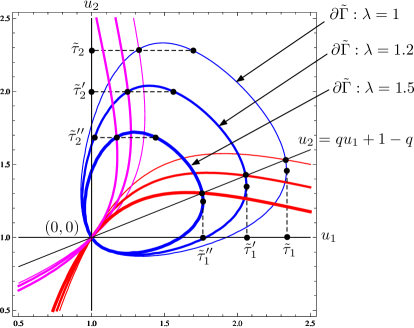
Figure 8: Effect of the arrival rate: $\lambda$ is changed from $1$ to $1.2$ and $1.5$ (thicker curves) while $\mu_{1}=5$, $\mu_{2}=4$, $p=0.25$, $q=0.4$ are unchanged

To circumvent this difficulty, we propose to draw figures. Nowadays we have excellent software such as Mathematica to draw two dimensional figures. Then, we can manipulate figures, and may find how modeling parameters change the tail asymptotics. This is essentially the same as numerical computations. However, figures are more informative to see how changes occur (see, e.g., Figure 8).

We finally consider a simpler case to find analytically tractable results. Assume that $q=0$ but $p>0$. $q=0$ implies that

$$\vec{u}^{(1,{\rm r})}=(\rho_{1}^{-1},1),$$

where $\rho_{1}=\frac{\lambda_{1}}{\mu_{1}}$. Obviously, $\rho_{1}$ must the decay rate of $P(L_{1}\geq n)$. This can be also verified by Theorem 4.3. However, it may not be the decay rate of $P(L_{1}\geq n,L_{2}=0)$. In fact, we can derive on the curve $\tilde{\gamma}_{+}(\vec{u})=1$,

$$\left.\frac{du_{1}}{du_{2}}\right|_{\vec{u}=\vec{u}^{(1,{\rm r})}}=\frac{\mu_{2}-(\mu_{1}+\lambda p)}{\lambda(1-\rho_{1}^{-1})}.$$

Hence, $u^{(1,{\Gamma})}_{1}=u^{(1,{\rm r})}_{1}$ if and only if

$$\mu_{2}\geq\mu_{1}+\lambda p_{1}.$$ (89)

Thus, if (89) holds, then $P(L_{1}\geq n,L_{2}=0)$ has the exactly geometric asymptotic. Otherwise, we have, by Theorem 4.1,

$$\lim_{n\to\infty}n^{-\frac{3}{2}}(u^{(1,\max)}_{1})^{-n}P(L_{1}\geq n,L_{2}=0)=b.$$ (90)

We can see that $\rho_{1}^{-1}<u^{(1,\max)}_{1}$, but $u^{(1,\max)}_{1}$ is only numerically obtained by solving (87) and (88).

7 Concluding remarks

We derived the exact asymptotics for the stationary distribution applying the analytic function method based on the convergence domain. We here discuss which problems can be studied by this method and what are needed for further developing it.

• In the analytic function method, a key ingredient is that the function $\underline{\zeta}_{2}(z)$ is analytic and suitably bounded for an appropriate region as we have shown in Lemma 8. For this, we use the fact that $\underline{\zeta}_{2}(z)$ is the solution of a quadratic equation, which is equivalent for the random walk to be skip free in the interior of the quadrant. The quadratic equation (or polynomial equation in general) is also a key for the alternative approach based on analytic extension on Riemann surface. If the random walk is not skip free, it would be harder to get a right analytic function. However, the non skip free case is also interesting. Thus, it is challenging to overcome this difficulty. One here may need a completely different approach.

• We have employed the purely analytic method, and gave no stochastic interpretations except a few although the asymptotic results are stochastic. However, probabilistic interpretations may be helpful. For example, one may wonder what are probabilistic meaning of the function $\underline{\zeta}_{2}$ and the equation (32). We do believe something should be here. If they are well answered, then we may better explain Lemma 8, and may resolve the technical issues discussed above.

• We think the present approach is applicable for a higher dimensional model as well as a generalized reflecting random walk proposed in Miyazawa 2011 as long as the skip free assumption is satisfied. One may also consider to relax the irreducibility condition on the random walk in the interior of the quadrant. However, this is essentially equivalent to reducing the dimension, so there should be no difficulty to consider it. Another extension is to modulate the double QBD or multidimensional reflecting random walk in general by a background Markov chain. The tail asymptotic problem becomes harder, but there should be a way to use the present analytic function approach at least for the two dimensional case with finitely many background states. Related discussions can be found in Miyazawa 2011 .

• As we have seen in Section 6, analytic results on the tail asymptotics may not be easy to apply for each specific application because they are not analytically tractable. To fill this gap between theory and application, we have proposed to use geometric interpretations instead of analytic formulas. However, this is currently more or less similar to have numerical tables. We here should make clear what we want to do using the tail asymptotics. Once a problem is set up, we may consider to solve it using geometric interpretations. Probably, there would be a systematic way for this not depending on a specific problem. This is also challenging.

Appendix

A. Proof of Lemma 6

Note that $u^{2}D_{2}(u)$ is polynomial with order 2 at least and order 4 at most. For $k=1,3$, let $c_{k}$ be the coefficients of $u^{k}$ in the polynomial $u^{2}D_{2}(u)$. Then,

$$c_{1}=-2(1-p_{00})p_{(-1)0}-4(p_{(-1)(-1)}p_{01}+p_{(-1)1}p_{0(-1)})\leq 0,$$

$$c_{3}=-2(1-p_{00})p_{10}-4(p_{1(-1)}p_{01}+p_{11}p_{0(-1)})\leq 0.$$

Hence, if both of $u^{(1,\max)}_{1}$ and $-u^{(1,\max)}_{1}$ are the solutions of $u^{2}D_{2}(u)=0$, then

$$2(c_{1}u^{(1,\max)}_{1}+c_{3}(u^{(1,\max)}_{1})^{3})=(u^{(1,\max)}_{1})^{2}(D_{2}(u^{(1,\max)}_{1})-D_{2}(-u^{(1,\max)}_{1}))=0.$$

Since $u^{(1,\max)}_{1}>0$, this holds true if and only if $c_{1}=c_{3}=0$, which is equivalent to that $p_{01}=p_{0(-1)}=p_{(-1)0}=p_{10}=0$ because $p_{00}=1$ is impossible. Hence, $u^{2}D_{2}(u)=0$ has the two solutions $u^{(1,\max)}_{1}$ and $-u^{(1,\max)}_{1}$ if and only if (v-a) does not hold. In this case, we have $c_{1}=c_{3}=0$, which implies that $u^{2}D_{2}(u)$ is an even function. Since $u^{2}D_{2}(u)=0$ has only real solutions including $u^{(1,\max)}_{1}$ by Lemmas 4 and 5, we complete the proof. ∎

B. Proof of Lemma 7

By (20), we have

$$\sum_{i\in\{-1,0,1\}}\sum_{j\in\{-1,0,1\}}p_{ij}x^{i}y^{j}=1,\qquad\sum_{i\in\{-1,0,1\}}\sum_{j\in\{-1,0,1\}}(-1)^{i+j}p_{ij}x^{i}y^{j}=1.$$

Subtracting both sides of these equations, we have

$$p_{10}x+p_{01}y+p_{0(-1)}y^{-1}+p_{(-1)0}x^{-1}=0.$$

Since $x,y$ are positive, this equation holds true if and only if

$$p_{10}=p_{01}=p_{0(-1)}=p_{(-1)0}=0.$$

This is the condition that (v-a) does not hold. ∎