Complex Faraday depth structure of Active Galactic Nuclei as revealed by broadband radio polarimetry

Abstract

We present a detailed study of the Faraday depth structure of four bright ($>1$ Jy), strongly polarized, unresolved, radio-loud quasars. The Australia Telescope Compact Array (ATCA) was used to observe these sources with 2 GHz of instantaneous bandwidth from 1.1 to 3.1 GHz. This allowed us to spectrally resolve the polarization structure of spatially unresolved radio sources, and by fitting various Faraday rotation models to the data, we conclusively demonstrate that two of the sources cannot be described by a simple rotation measure (RM) component modified by depolarization from a foreground Faraday screen. Our results have important implications for using background extragalactic radio sources as probes of the Galactic and intergalactic magneto-ionic media as we show how RM estimations from narrow-bandwidth observations can give erroneous results in the presence of multiple interfering Faraday components. We postulate that the additional RM components arise from polarized structure in the compact inner regions of the radio source itself and not from polarized emission from Galactic or intergalactic foreground regions. We further suggest that this may contribute significantly to any RM time-variability seen in RM studies on these angular scales. Follow-up, high-sensitivity VLBI observations of these sources will directly test our predictions.

1 Introduction

Radio-loud Active Galactic Nuclei (AGN) eject powerful jets of relativistic plasma whose polarized, non-thermal synchrotron radiation can be used as a probe of the magneto-ionic material along the entire line of sight between us and the source of emission. Many studies have used these extragalactic background sources to study the strength and structure of magnetic fields in our Galaxy (e.g. Brown et al., 2007; Taylor et al., 2009; Mao et al., 2010; Van Eck et al., 2011; Harvey-Smith et al., 2011), other galaxies (e.g. Gaensler et al., 2005; Mao et al., 2008; Feain et al., 2009) and in galaxy clusters (e.g. Laing et al., 2008; Bonafede et al., 2010; Pizzo et al., 2011). Future studies on new revolutionary instruments such as the Australian Square Kilometre Array Pathfinder (ASKAP) and the Square Kilometre Array (SKA) will rely on these background sources to probe the strength, structure and evolution of cosmic magnetism in unprecedented detail (e.g. Beck & Gaensler, 2004; Gaensler, 2009).

In this paper, we present a detailed study of the polarization and rotation measure (RM) properties of four bright, unresolved, strongly polarized, radio–loud AGN. Using the new Compact Array Broadband Backend (CABB) system (Wilson et al., 2011) on the Australia Telescope Compact Array (ATCA), spectropolarimetric studies of these AGN were performed using 2 GHz of instantaneous bandwidth on the upgraded receiver system from 1.1 to 3.1 GHz. All-sky RM surveys such as the planned Polarization Sky Survey of the Universe’s Magnetism (POSSUM) on ASKAP will measure the RMs of $\sim 3$ million extragalactic radio sources over 30,000 deg² (Gaensler et al., 2010). POSSUM will likely have 300 MHz of instantaneous bandwidth covering the frequency range from 1130 to 1430 MHz. Proper interpretation of the results from this huge dataset will require extensive testing of the algorithms used to accurately extract the polarization and RM properties of individual sources. The ATCA is an ideal instrument for this process, whilst also providing new and unique insights into the Faraday depth structure of extragalactic sources due to its wide-bandwidth and high spectral resolution.

Following Sokoloff et al. (1998), and references therein, we define the complex linear polarization as

$$P=Q+iU=pIe^{2i\Psi}$$ (1)

where $I$, $Q$, $U$ are the measured Stokes parameters and $\Psi$ is the observed polarization angle. We use the notation of Farnsworth et al. (2011) in defining $q=Q/I$ and $u=U/I$, so that the measured magnitude of the degree of linear polarization is

$$p=\sqrt{q^{2}+u^{2}}$$ (2)

and the polarization angle is

$$\Psi=\frac{1}{2}\arctan\frac{u}{q}$$ (3)

Taking the fractional values decouples depolarization effects from simple spectral index effects in analysing the dependence of polarization with wavelength. It also minimises errors in the estimate of the RM using the RM synthesis technique (Brentjens & de Bruyn, 2005).

The observed polarization angle $\Psi$ is modified from its intrinsic value ($\Psi_{0}$) by the effect of Faraday rotation, caused by magneto-ionic material between the source of polarized emission and the telescope. If there are different regions of polarized emission sampled within a single resolution element then each of these regions will likely experience different amounts of Faraday rotation. Hence, to describe the Faraday rotation of a particular region of polarized emission we use the Faraday depth (Burn, 1966)

$$\phi=0.81\int^{\rm telescope}_{\rm emission}{n\mn@boldsymbol{B}\cdot d\mn@boldsymbol{l}}~{}~{}{\rm rad~{}m}^{-2}$$ (4)

where $n$ is the free electron density (in units of cm^-3), $\mn@boldsymbol{B}$ is the magnetic field (in $\mu$G) and $\mn@boldsymbol{l}$ is the distance along the line of sight (in parsecs). Brentjens & de Bruyn (2005) define a “Faraday thin” source as one in which $\lambda^{2}\Delta\phi\ll 1$, and a “Faraday thick” source in cases where $\lambda^{2}\Delta\phi\gg 1$ (where $\Delta\phi$ is the extent of the source in Faraday depth and $\lambda$ is the wavelength).

In the simplest possible scenario, in which there is a background source of emission and only pure rotation due to a foreground magneto-ionic medium, then the Faraday depth is equal to the RM and we get

$$\Psi=\Psi_{0}+{\rm RM}\,\lambda^{2}$$ (5)

Depolarization from radio sources, where the degree of polarization decreases with increasing wavelength, is typically modelled as a single RM component with external Faraday dispersion (e.g. Tribble, 1991; Rossetti et al., 2008). Our new wide-bandwidth data allow a detailed investigation of the case of multiple interfering RM components either along the line of sight or intrinsic to the source itself. Multiple RM components can cause both increases and/or decreases in $p(\lambda^{2})$ with $\lambda^{2}$ as well as, but not always, deviations from a linear $\Psi(\lambda^{2})$ behaviour. Slysh (1965) first employed a two component model to explain polarization measurements of Cygnus A while Goldstein & Reed (1984) applied a similar model to 3C 27. A more recent study by Law et al. (2011) showed that multiple RM components could be identified in extragalactic point sources using the RM synthesis technique on wide-band data from 1.0 to 2.0 GHz. Farnsworth et al. (2011) highlighted the importance of describing both $\Psi(\lambda^{2})$ and $p(\lambda^{2})$ in determining the correct Faraday depth structure of extragalactic sources using a combination of data at 350 MHz and 1.4 GHz. Following on from this work, we conclusively show the effect of multiple RM components in two extragalactic sources by considering several different Faraday rotation models to simultaneously describe both $\Psi(\lambda^{2})$ and $p(\lambda^{2})$.

In Section 2, we describe the observations, source selection and calibration process. Section 3 outlines the RM synthesis technique while Section 4 describes the various polarization models employed as well as our method for discriminating between models. Section 5 presents our results for each source in order of increasing RM complexity. Section 6 discusses the implications of this work and we list our conclusions in Section 7. Throughout this paper, we assume a cosmology with H${}_{0}=71$ km s^-1 Mpc^-1, $\Omega_{M}=0.27$ and $\Omega_{\Lambda}=0.73$, and define the spectral index, $\alpha$, such that the observed flux density ($I$) at frequency $\nu$ follows the relation $I_{\nu}\propto\nu^{\rm{+}\alpha}$.

2 Observations and Data Reduction

Table 1: Observed sources (listed in order of increasing RM complexity)

(1)	(2)	(3)	(4)	(5)	(6)	(7)	(8)	(9)	(10)	(11)	(12)	(13)
Source	RA	DEC	$l$	$b$	beam	pa	$z$	Date	$t_{\rm obs}$	$\lambda_{0}$	$I_{\lambda_{0}}$	$\alpha$
Name	[J2000]	[J2000]	[∘]	[∘]	[$"\times"$]	[∘]			[min]	[m]	[mJy]
PKS B1903-802	19:12:40.0	-80:10:05.9	314.0	$-27.6$	$11\times 9$	$-10$	0.50	2011-01-20	23	0.141	1104	$-0.04$
PKS B0454-810	04:50:05.4	-81:01:02.2	293.9	$-31.4$	$12\times 9$	$+60$	0.44	2011-01-20	16	0.108	1009	$+0.46$
PKS B1610-771	16:17:49.2	-77:17:18.5	313.4	$-18.9$	$10\times 9$	$+30$	1.71	2011-01-20	12	0.137	3022	$-0.36$
PKS B1039-47	10:41:44.6	-47:40:00.1	281.4	$+9.7$	$12\times 9$	$0$	2.59	2011-01-09	22	0.164	1699	$-0.38$

Column designation: 1 - Source name (IAU B1950.0); 2 - Right Ascension in J2000 coordinates; 3 - Declination in J2000 coordinates; 4 - Galactic longitude in degrees; 5 - Galactic latitude in degrees; 6 - Synthesised beam in arcseconds; 7 - Synthesised beam position angle in degrees; 8 - redshift, taken from Stickel et al. (1994), and references therein, except for PKS B1039-47 (O. Titov, private communication); 9 - Date of observations; 10 - Total integration time in minutes; 11 - Weighted mean $\lambda$; 12 - Total intensity at $\lambda_{0}$; 13 - Spectral index ($\alpha$), defined as $I_{\lambda}\propto\lambda^{-\alpha}$, calculated from our observations.

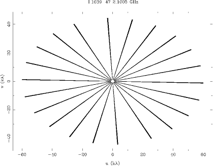
Figure 1: Plot showing the typical $uv$-coverage for the sources presented in this paper (PKS B1039-47 shown).

The sources presented in this paper (Table 1) were observed on 9 Jan 2011 and 20 Jan 2011 with the ATCA from 1.1–3.1 GHz (with 1 MHz spectral resolution) in the 6A array configuration as part of a larger project to find suitable polarization calibrator sources for the ASKAP telescope. Figure 1 shows the typical $uv$-coverage for sources in our experiment. The ATCA has six 22m antennas with linear feeds and a maximum baseline of 6 km providing an angular resolution of $\sim$10” at 1.4 GHz. It has recently undergone a major upgrade with the capabilities of the new CABB system described in detail by Wilson et al. (2011).

Since there are no 1.4 GHz polarization surveys of the southern sky at a resolution better than 36^′ (Testori et al., 2008), we compiled a list of sources suitable for ASKAP polarization calibration from archival observations. Candidate sources were selected by searching the ATCA online archive for sources that had Stokes I flux densities greater than 1 Jy at 843 MHz in the SUMSS catalogue (Mauch et al., 2003). The extracted sources, which had been observed using the old narrow-band 128 MHz system, were then calibrated and imaged in Miriad using standard techniques (Sault et al., 1995). Eight of the brightest sources found in polarized intensity were selected along with two unpolarized sources (fractional polarization $<0.1$%) for high precision polarization observations with the new wide-band CABB system on the ATCA. We selected four sources for detailed analysis in this paper that had reliable calibration across the full 2 GHz band and displayed a range of RM complexity from single to multiple RM components.

In order to avoid any frequency-dependent calibration effects, the data for each source were split up at 128 MHz intervals and calibrated using the Miriad software package. For the absolute flux density scale correction and bandpass calibration, we used a single observation of the ATCA primary flux calibrator PKS B1934-638 on each day. Flagging was done in an automated fashion (after bandpass calibration) using Mirflag (Middelberg, 2006). Some minor manual flagging was sometimes required afterwards. In total $\sim$$10-30\%$ of the 2 GHz band was lost due to radio-frequency interference (RFI), mainly between 1.1 and 1.7 GHz. The leakage and complex gain solutions were determined for each individual 128 MHz sub-band before recombining the entire band.

One of our targets, PKS B1903-802, was used on 20 Jan 2011 as the secondary calibrator to correct for any atmospheric phase variations as well as the polarization leakages (21 x 1 min cuts, with one cut approximately once every hour, covering $340^{\circ}$ of parallactic angle). Because PKS B1903-802 is strongly polarized across the entire 2 GHz band, the $XY$ phase variations on the reference antenna could be determined and we were able to calibrate the absolute polarization position angle to within $\pm 1^{\circ}$. These solutions were then copied to the other sources and amplitude and phase self-calibration was performed on PKS B0454-801 and PKS B1610-771. Our other target, PKS B1039-47, was used for polarization calibration on 9 Jan 2011 (11 x 2 min cuts every hour, with a parallactic angle coverage of $210^{\circ}$).

Our calibration strategy allowed us to calculate the on-axis leakages in 128 MHz intervals. The results show that the real part of the leakage solution, which gives information about how the linear feeds deviate from perfect orthogonality (feed misalignment), is constant to better than 0.5% across the entire band. The imaginary part, which probes the feed ellipticity (i.e. how the feeds differ from perfectly linear feeds), has maximum deviations of up to $\sim 2\%$ between 1.2 and 1.8 GHz. We find little variation between the leakage solutions on different days suggesting that the polarization performance of the wide-bandwidth system is stable on timescales of at least a few weeks.

3 Extracting the Polarized Signal

We first created uniformly-weighted $I$, $Q$ and $U$ images for each source in 10 MHz intervals and then deconvolved these maps using the Högbom CLEAN algorithm (Högbom, 1974). In order to avoid any resolution dependent effects across the 2 GHz band, we smoothed each image to the resolution at the lowest frequency (see Table 1). Since all sources were spatially unresolved, we took the emission at the position of the source in the Stokes $I$ image and created a table of $q$ and $u$ as a function of $\lambda^{2}$, at intervals in $\lambda^{2}$ corresponding to 10 MHz steps. Errors in each channel measurement were assigned using the rms noise from a small area around the source position in the clean-residual images.

We then used the RM synthesis technique (Brentjens & de Bruyn, 2005) to extract the polarized signal over a wide range of possible Faraday depths. RM synthesis is a powerful analysis tool for polarimetry data since it helps overcome problems such as bandwidth depolarization and $n\pi$ polarization angle ambiguities. A spectrum of complex polarization versus Faraday depth was created from these data using the equation

$$F(\phi)=\sum^{N}_{j=1}w_{j}P_{j}e^{-2i\phi(\lambda_{j}^{2}-\lambda_{0}^{2})}\Big{/}\sum^{N}_{j=1}w_{j}$$ (6)

where $N$ is the number of input maps, $P_{j}$ is the complex polarization at channel $j$ and $w_{j}$ are the weights (inverse square of the rms noise). Our reference wavelength ($\lambda_{0}$) is defined as

$$\lambda_{0}^{2}=\sum^{N}_{j=1}w_{j}\lambda^{2}_{j}\Big{/}\sum^{N}_{j=1}w_{j}.$$ (7)

Essentially this derotates the $q$ and $u$ data for a particular assumed RM value and then sums the signal across the band; at the correct RM, the channels add coherently giving the maximum polarized intensity and the sensitivity of the full bandwidth.

Figure 2 shows the Rotation Measure Spread Function (RMSF) for the observations on both days. The RMSF is the normalised response function in Faraday depth space to the incomplete $\lambda^{2}$-sampling (i.e. with perfect $\lambda^{2}$ coverage this would be a delta function). More data were flagged on 9 Jan 2011 than on 20 Jan 2011, so that the RMSF for 9 Jan has slightly stronger sidelobes than on 20 Jan. Table 2 lists, for our observations, the Faraday depth resolution ($\delta\phi\approx 2\sqrt{3}/\Delta(\lambda^{2})$, i.e. the FWHM of the RMSF), the largest detectable scale in Faraday depth space (max-scale $\approx\pi\lambda_{\rm min}^{-2}$) and the maximum observable Faraday depth ($\phi_{\rm max}\approx\sqrt{3}/\delta\lambda^{2}$), where $\Delta(\lambda^{2})$ is the total bandwidth in $\lambda^{2}$-space (i.e. $\Delta(\lambda^{2})=\lambda^{2}_{\rm max}-\lambda^{2}_{\rm min}$) and $\delta\lambda^{2}$ is the channel width.

For each source, we initially searched for polarized power from $\pm\phi_{max}$ at Faraday depth intervals of 10 rad m^-2 which corresponds to $\sim$6 Faraday depth intervals per $\delta\phi$ (see Table 2). No significant power was found at large values of $|\phi|$. For the rest of our analysis we restricted our range to $\pm 1000$ rad m^-2 at 1 rad m^-2 intervals ($\sim 60$ Faraday depth intervals per $\delta\phi$). We use RMCLEAN, as described by Heald et al. (2009), to deconvolve the “dirty” RM spectrum in an attempt to recover information lost due to the incomplete frequency coverage. For each source, we cleaned down to the rms noise level ($\sigma_{q,u}$) listed in Table 3. In principle, the RM synthesis technique should be able to detect regions that are extended in Faraday depth space as long as the region extends beyond the FWHM of the RMSF.

Table 2: RM Synthesis Capabilities of 1.1–3.1 GHz ATCA band

(1)	(2)	(3)	(4)	(5)
Frequency	Resolution	$\delta\phi$	max-scale	$|\phi_{max}|$
${\rm[GHz]}$	[MHz]	[rad m-2]	[rad m-2]	[rad m-2]
1.1–3.1	1.0	60	340	13000

Column designations: 1 - Instantaneous frequency coverage in GHz; 2 - Spectral resolution in MHz; 3 - Resolution in Faraday depth space; 4 - maximum detectable Faraday thickness; 5 - Maximum detectable Faraday depth.

4 Modelling Procedure

To model the polarized signal in the presence of Faraday rotation in the simplest case, we use the equation

$$P=p_{0}e^{2i(\Psi_{0}+{\rm RM}\lambda^{2})}$$ (8)

where $p_{0}$ is the intrinsic degree of polarization of the synchrotron emission, $\Psi_{0}$ is the intrinsic polarization angle at the source of the emission and the RM describes the Faraday rotation caused by the foreground magneto-ionic material with the sign indicating whether the line-of-sight magnetic field is pointing towards us (positive RM) or away from us (negative RM). The data for all our sources show changes in the degree of polarization across the observed wavelength range so we now consider the possible mechanisms behind this effect.

Depolarization towards longer wavelengths can occur due to mixing of the emitting and rotating media, as well as from the finite spatial resolution of our observations. There are three commonly listed depolarization mechanisms (see Sokoloff et al. (1998) for more detailed discussion of each case).

1. Differential Faraday rotation (DFR): this occurs when the emitting and rotating regions are co-spatial and are in the presence of a regular magnetic field. The polarization plane of the emission at the far side of the region undergoes a different amount of Faraday rotation compared to the polarized emission coming from the near side, causing depolarization when summed over the entire region. For the particular case of a uniform slab we have

$$P=p_{0}\frac{\sin{R}\lambda^{2}}{{R}\lambda^{2}}e^{2i(\Psi_{0}+\frac{1}{2}{R}\lambda^{2})}$$ (9)

where $R$ is the Faraday depth through the region.

2. Internal Faraday dispersion (IFD): this occurs when the emitting and rotating regions also contain a turbulent magnetic field. In this case depolarization occurs because the plane of polarization experiences a random walk through the region. For identical distributions of all the constituents of the magneto-ionic medium along the line of sight, it can be described by

$$P=p_{0}e^{2i\Psi_{0}}\left(\frac{1-e^{2i{R}\lambda^{2}-2\varsigma^{2}_{\rm RM}\lambda^{4}}}{2\varsigma^{2}_{\rm RM}\lambda^{4}-2i{R}\lambda^{2}}\right)$$ (10)

where, in this case, $\Psi_{0}=\pi/2$ for a purely random anisotropic magnetic field and $\varsigma_{\rm RM}$ is the internal Faraday dispersion of the random field.

3. External Faraday dispersion/beam depolarization: this occurs in a purely external, non-emitting Faraday screen. In the case of turbulent magnetic fields, depolarization occurs when many turbulent cells are within the synthesised telescope beam. On the other hand, for a regular magnetic field, any variation in the strength or direction of the field within the observing beam will lead to depolarization. Both effects can be described by

$$P=p_{0}e^{-2\sigma^{2}_{\rm RM}\lambda^{4}}e^{2i(\Psi_{0}+{\rm RM}\lambda^{2})}$$ (11)

where $\sigma_{\rm RM}$ is the dispersion about the mean RM across the source on the sky.

A fourth possibility is a changing degree of polarization due to multiple interfering RM components, either along the line of sight or on the plane of the sky on scales smaller than our spatial resolution.

To model our data, we simultaneously fit both the $q(\lambda^{2})$ and $u(\lambda^{2})$ data to the different polarization models listed above. We first tried a simple one-component RM model, which cannot describe any variation in the degree of polarization. We then tried to account for changes in $p(\lambda^{2})$ by fitting a single RM component plus depolarization model, and in cases where this could not adequately describe the data, we then tried multiple RM-component models. In order to limit the number of models to investigate, we mainly considered models of either solely Faraday thin components (e.g. emission from the radio galaxy only) or models of one Faraday thick component (e.g. Galactic slab or mixed emitting and rotating region in the source) plus Faraday thin component(s). We believe that these models are the most physically reasonable cases for spatially unresolved extragalactic radio sources. However, we do not consider differing spectral indices of individual components. Hence, multiple component models are simply constructed as $P=P_{1}+P_{2}+\dots+P_{N}$.

4.1 Model-fit Evaluation

We utilised the maximum likelihood method to find the best-fit model parameters. The results from RM synthesis were used as a guide to our initial guesses for the RM and fractional polarization values. Each data point in the fit was weighted by the inverse square of the rms noise from the clean-residual image.

The likelihood is the probability of obtaining the data, $d$, given a model of the source and some characterisation of the noise. Our data in this context are $q(\lambda^{2})$ and $u(\lambda^{2})$. For example, in the one-component model, we adopt $q_{model,i}=p_{0}\cos(2\Psi_{0}+2{\rm RM}\lambda_{i}^{2})$ and $u_{model,i}=p_{0}\sin(2\Psi_{0}+2{\rm RM}\lambda_{i}^{2})$, and we assume that $q_{i}=q_{model,i}+n_{i}$, where $n_{i}$ is Gaussian noise for channel $i$. The prior likelihood of a particular RM value for an observation of a single channel $i$ under the assumption of Gaussian noise is

$$P_{i}(d_{i}|{\rm RM})=\frac{1}{\pi\sigma_{q_{i}}\sigma_{u_{i}}}\exp{\left(-\frac{(q_{i}-q_{model,i})^{2}}{2\sigma_{q_{i}}^{2}}-\frac{(u_{i}-u_{model,i})^{2}}{2\sigma_{u_{i}}^{2}}\right)}$$ (12)

where $\sigma_{q,u}$ is the single channel rms. If we have a total of $N$ channels, the prior likelihood is now

$$P(d|{\rm RM})=\prod_{i=1}^{N}P_{i}(d_{i}|{\rm RM})$$ (13)

We used the Mathematica function Nonlinearmodelfit to find the maximum of Eqn. 13, $L\equiv max(P(d|{\rm RM}))$. In the case of multiple models giving good fits to the data, we then used the Bayesian Information Criterion (BIC) to distinguish the goodness-of-fit between different models with different degrees-of-freedom (Schwarz, 1978; Trotta, 2008);

$${\rm BIC}\equiv-2\log P(d|k)\approx-2\log L+k\log N$$ (14)

where $k$ is the number of free parameters in the model. Hence, models with more parameters are heavily penalised given the large number of data points. We consider ${\rm BIC_{model_{1}}}-{\rm BIC_{model_{2}}}>100$ to significantly favour model 2 (at 99% level) across the measured parameter space. Bayesian model comparisons require an alternative model against which the comparison is made (i.e. a model cannot be rejected unless an alternative explanation is available that better fits the observations). In order to give a quantitative measure of how each individual model fits the data, we also calculate the reduced chi-square ($\chi^{2}_{\nu}$) goodness-of-fit values, where $\chi^{2}_{\nu}$ is obtained by dividing the sum of squared residuals by $\sigma_{q,u}^{2}$ and the number of degrees of freedom.

5 Results

We present the sources in order of RM complexity (as listed in Table 1) with PKS B1903-802 having the simplest RM structure and PKS B1039-47 having the most complex. All models with their best-fit parameters for each source are listed in Table 3 (with the most-likely model highlighted in bold). The associated errors of each parameter are formal fitting errors which are calculated from the square root of the estimated error variance of each parameter. These errors have little meaning when the incorrect model is applied. Note that all polarized components listed are found with high significance. For example, the weakest polarized model component of 0.6% listed in Table 3 has a signal to noise ratio (SNR) of $\sim$100.

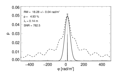
(a) PKS B1903-802

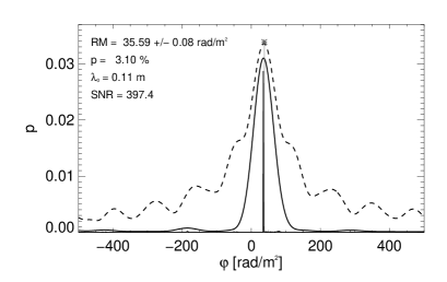
(b) PKS B0454-810

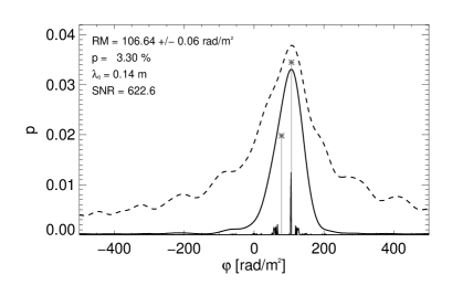
(c) PKS B1610-771

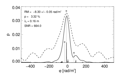
(d) PKS B1039-47

Figure 3: Plots of the RM spectra for all four sources. Dashed line: RM synthesis spectrum. Solid line: RMCLEAN spectrum with the locations of the clean-components also shown as vertical lines. The text in the top-left corner of each panel lists the parameters extracted from the peak in the RMCLEAN spectrum as well as the value of the reference wavelength, $\lambda_{0}$. The asterisks connected to the Faraday depth axis by the solid line denote the locations of the best-fit model RM.

In Figure 3, we show the results of RM synthesis and RMCLEAN for all four sources. For each source we list the RM at the peak degree of polarization with its associated error. The uncertainty in the peak RM is calculated as the FWHM of the RMSF divided by twice the SNR (Brentjens & de Bruyn, 2005). So for example, if we have an SNR of 600 and an RM resolution of $66$ rad m^-2, then the quoted uncertainty in the peak RM is $0.06$ rad m^-2. However, as described by Law et al. (2011), the accuracy of any individual RM-component value cannot be specified to better than the RM resolution due to the uncertainty in the distribution of components within the RM beam. The mean-weighted reference wavelength ($\lambda_{0}$) changes from source to source mainly due to different amounts of flagged data across the band for each source.

Faraday depth spectra for both PKS B1903-802 (Fig. 3a) and PKS B0454-810 (Fig. 3b) appear to be broadly consistent with a single RM component. The asymmetric distribution about the peak for PKS B1610-771, as well as the distribution of clean-components, indicates the presence of more than one RM component (Fig. 3c). PKS B1039-47 has a distinct secondary peak at $\sim$100 rad m^-2 and the clean-component locations suggest the presence of three or more RM components (Fig. 3d) . We now discuss the Faraday rotation model-fits to the $q(\lambda^{2})$, $u(\lambda^{2})$ data for each source which are completely independent of the RMCLEAN results.

5.1 PKS B1903-802

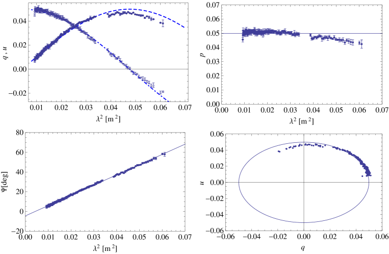
Figure 4: Polarization data for PKS B1903-802, and the corresponding best-fit single RM-component model. (Eqn. 8). Top left: $q$ (open circles) and $u$ (full circles) data vs. $\lambda^{2}$, fitted with the model $q$ (dot-dashed line) and $u$ (dashed line). Top right: $p$ vs. $\lambda^{2}$ data over-plotted by the model (solid line). Bottom left: $\Psi$ vs. $\lambda^{2}$ data over-plotted by the model (solid line). Bottom right: $u$ vs. $q$ data over-plotted by the model (solid line).

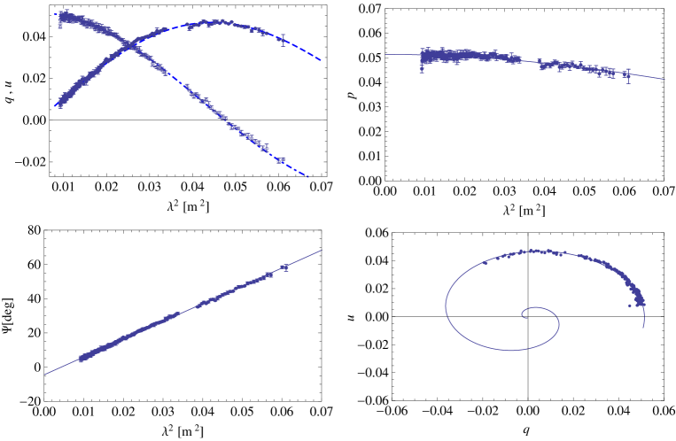
Figure 5: As for Figure 4 for PKS B1903-802, but now modelled by a single RM-component model with depolarization from external Faraday dispersion (Eqn. 11).

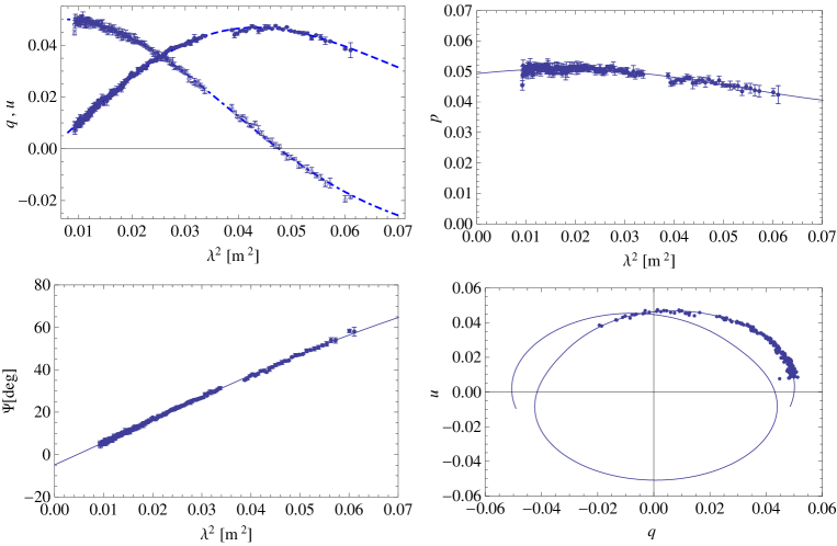
Figure 6: As for Figure 4 for PKS B1903-802, but fit with a two RM-component model.

A simple RM fit (Eqn. 8), as shown in Figure 4, provides a reasonable description of the $\Psi(\lambda^{2})$ data but the $p$ vs. $\lambda^{2}$ data clearly deviates from a constant degree of polarization. An external Faraday dispersion model (Eqn. 11) provides an excellent fit to data, with our best fit model, shown in Figure 5, giving a polarized intensity of $5.14\pm 0.04\%$, with a foreground RM of $+18.1\pm 0.1$ rad m^-2 and an external dispersion in RM across the source of $4.7\pm 0.1$ rad m^-2. However, in Figure 6 we can see that a two RM-component model also provides a very good description of the data with an RM of $+16.1\pm 0.3$ rad m^-2 for the stronger polarized component ($\sim$$4.5\%$) and an RM of 39.3$\pm 2.0$ rad m^-2 for the second polarized component ($\sim$$0.6\%$). This supports the conclusion of Farnsworth et al. (2011) that modelling of both polarization amplitude and polarization angle is required in studies of Faraday rotation.

In this case, neither the BIC nor the $\chi^{2}_{\nu}$ help us to clearly discriminate between models. The two models do not differ significantly over the measured parameter space so we cannot state with confidence which one is correct, although we favour the simpler external Faraday dispersion model. Lower frequency observations, from 700 MHz to 1 GHz on ASKAP for example, would clearly discriminate between the two models since for the two RM-component model there is a departure from a linear $\Psi$ vs. $\lambda^{2}$ relationship over this range. The difference can be seen most clearly in the $q(\lambda^{2})$ vs. $u(\lambda^{2})$ plots (i.e. compare Fig. 5 and Fig. 6).

Table 3.
(1)	(2)	(3)	(4)	(5)	(6)	(7)	(8)	(9)	(10)	(11)	(12)	(13)	(14)	(15)
Source	Model	RM1	$p_{01}$	$\Psi_{01}$	RM2	$p_{02}$	$\Psi_{02}$	RM3	$p_{03}$	$\Psi_{03}$	$\sigma_{\rm RM}$	$\sigma_{q,u}$	$\chi^{2}_{\nu}$	BIC
		[rad m-2]	[%]	[∘]	[rad m-2]	[%]	[∘]	[rad m-2]	[%]	[∘]	[rad m-2]	[%]
PKS B1903-802	Single RM, no screen	$+18.1(1)$	$4.98(1)$	$-4.4(1)$	-	-	-	-	-	-	-	0.006	1.23	$-3470$
	Single RM, foreground screen	$+18.1(1)$	$5.14(4)$	$-4.4(1)$	-	-	-	-	-	-	$4.7(1)$	-	1.03	$-3714$
	2 RM Components, no screen	$+16.1(3)$	$4.50(8)$	$-2.4(3)$	$+39(2)$	$0.59(8)$	$-25(2)$	-	-	-	-	-	1.04	$-3779$
PKS B0454-810	Single RM, no screen	$+37.9(2)$	$3.36(2)$	$-48.6(3)$	-	-	-	-	-	-	-	0.008	2.13	$-3250$
	Single RM, foreground screen	$+37.8(2)$	$3.39(2)$	$-48.6(3)$	-	-	-	-	-	-	$2.8(6)$	-	1.60	$-3250$
	2 RM Components, no screen	$+29(1)$	$2.7(2)$	$-33(2)$	$+62(3)$	$1.1(2)$	$+88(5)$	-	-	-	-	-	1.07	$-3548$
PKS B1610-771	Single RM, no screen	$+109.0(7)$	$3.79(7)$	$+69(1)$	-	-	-	-	-	-	-	0.005	97.3	$-2346$
	Single RM, foreground screen	$+104.3(4)$	$5.20(4)$	$+73.9(5)$	-	-	-	-	-	-	$17.3$ (0.3)	-	1.41	$-3024$
	2 RM Components, no screen	$+107.1(2)$	$3.45(4)$	$+83.3(6)$	$+78.7(4)$	$1.98(4)$	$+73(1)$	-	-	-	-	-	1.04	$-3845$
PKS B1039-47	Single RM, no screen	$-12.3(5)$	$3.43(5)$	$+18.8(8)$	-	-	-	-	-	-	-	0.005	127	$-2362$
	2 RM Components, no screen	$-9.8(4)$	$3.64(4)$	$+14.3(7)$	$+85(2)$	$0.68(4)$	$0(4)$	-	-	-	-	-	14.3	$-2524$
	3 RM Components, no screen	$-13(1)$	$3.9(4)$	$+31(4)$	$-30(2)$	$1.7(4)$	$0(8)$	$+68(2)$	$0.7(2)$	$+35(3)$	-	-	1.23	$-3194$
	3 RM Components (1 DFR)	$-13(4)$	$2.3(3)$	$+37(5)$	$+70(1)$	$0.7(2)$	$+33(3)$	$-21(4)$	$2.9(1)$	$+11(15)$	-	-	1.25	$-3192$

Column designation: 1 - Source name; 2 - Description of Faraday rotation model used; 3 - RM of first component ; 4 - Degree of polarization of first component; 5 - Intrinsic polarization angle (at $\lambda=0$) of first component; 6 - RM of second component ; 7 - Degree of polarization of second component; 8 - Intrinsic polarization angle of second component; 9 - RM of third component ; 10 - Degree of polarization of third component; 11 - Intrinsic polarization angle of third component; 12 - Dispersion about mean RM; 13 - rms noise level in fractional polarization; 14 - Reduced chi-square goodness-of-fit value; 15 - Bayesian information criterion for model comparison. The favoured model for each source is indicated by bold-face font. The error in the final digit of all parameters is indicated by the number in the parentheses.

5.2 PKS B0454-810

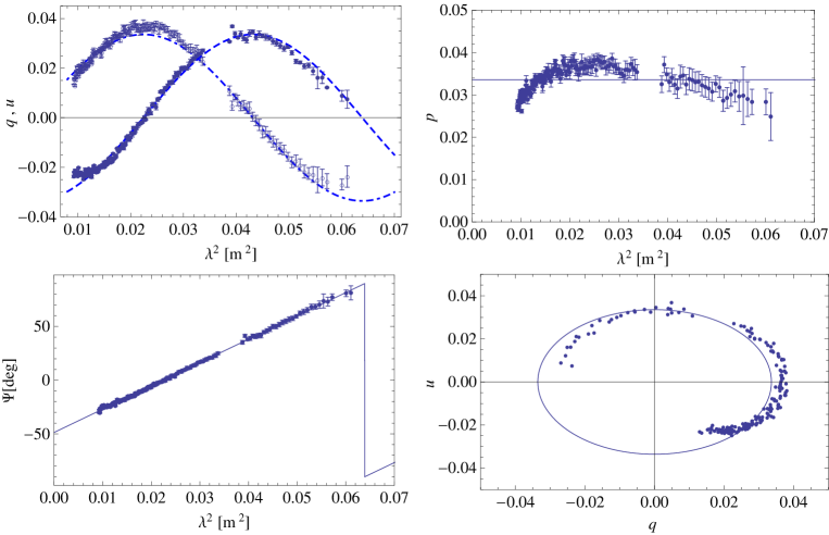
Figure 7: Polarization data for PKS B0454-810, and the corresponding best-fit single RM-component model (Eqn. 8). Layout as described in Figure 4.

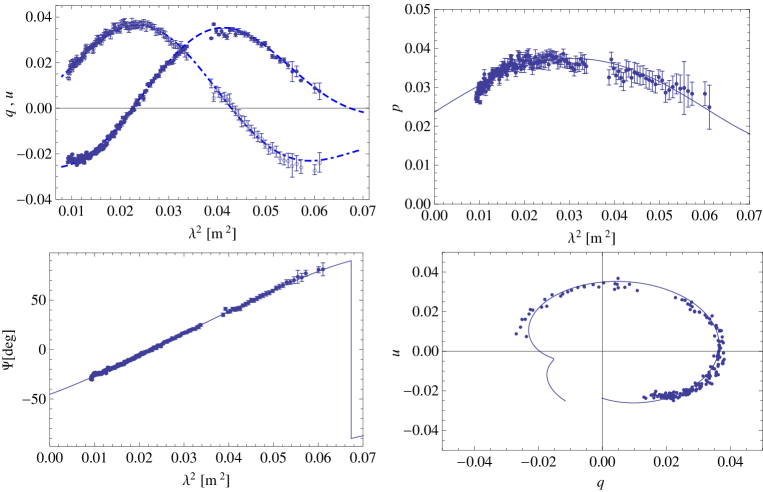
Figure 9: As for Figure 7 for PKS B0454-810, but fit with a two RM-component model. The kink in the $q(\lambda^{2})$ vs. $u(\lambda^{2})$ plot is a unique signature of this particular model.

As can be seen in Figures 7 & 8, both single-component RM models (with and without a depolarizing screen) provide poor fits to the data. They both determine approximately the same RM ($+37.8\pm 0.2$ rad m^-2) but cannot explain the observed decrease in the degree of polarization towards the shortest wavelengths. The two-component model, shown in Figure 9, does much better at describing the $p(\lambda^{2})$ data while also providing a good description of $\Psi(\lambda^{2})$. We note that the RM of the strongest polarized component is now significantly different ($+29.2\pm 1.1$ rad m^-2) from that found in the one-component models or from the peak in Faraday depth inferred from RM synthesis in Figure 3(b).

While both the reduced chi-squared and BIC values strongly favour the two RM-component model over the single component models (Table 3), on closer inspection it is clear that the $p(\lambda^{2})$ data at the shortest wavelengths observed are not very well fit by the two RM-component model either (Fig. 9). Hence, we conclude that the data are not well fit by any of the three models listed in Table 3.

We consider a possible alternative explanation for this source in terms of polarization propagation effects as a function of optical depth within the source. Specifically, the case of one optically thick and one optically thin component; the optically thin and strongly polarized component would dominate the emission at the longer wavelengths ($\lambda^{2}>0.025$ m²) while the observed depolarization could be explained by external Faraday dispersion. At the shorter wavelengths ($\lambda^{2}<0.025$ m²), the optically thick and weakly polarized component would become more dominant coupled with the optically thin component becoming fainter leading to a decrease of the observed degree of polarization in a non-trivial manner. This idea is supported by the inverted spectrum indicative of a synchrotron self-absorbed region caused by either multiple, discrete spectral components or a smooth distribution of magnetic field and electron density along the jet. If this model were correct, then we would expect at even shorter wavelengths, as the emission spectrum turns over, the degree of polarization should increase again. However, detailed modelling of the polarized radiative transfer from such a region is required for a quantitative analysis and we defer such a study for a later paper.

5.3 PKS B1610-771

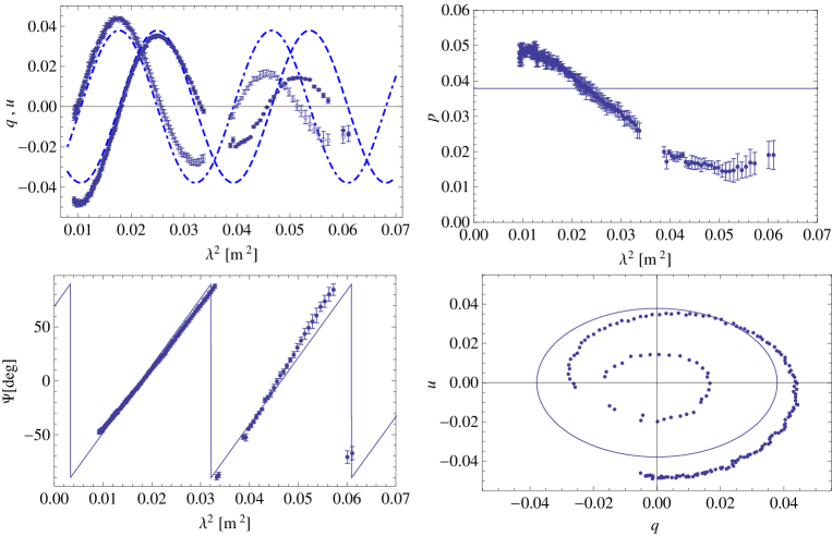
Figure 10: Polarisation data for PKS B1610-771, and the corresponding best-fit single RM-component model (Eqn. 8). Layout as described in Figure 4.

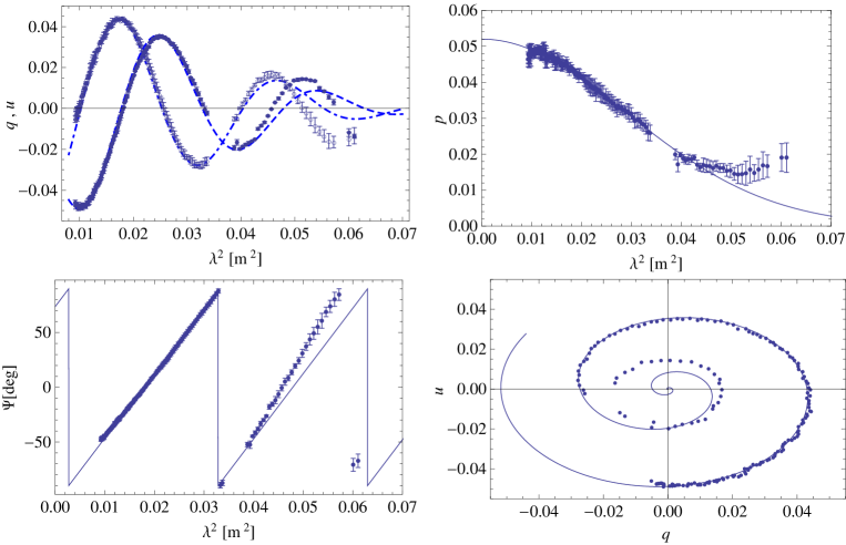
Figure 11: As for Figure 10 for PKS B160-771, but fitted by a single RM-component model with depolarization from external Faraday dispersion (Eqn. 11).

Figure 10 shows how a simple one-component model provides a very poor fit to the complex polarization data for this source. A depolarizing screen model, shown in Figure 11, gives a good fit at the short wavelengths but fails to adequately fit the long wavelength data. These plots further highlight two interesting features of the data. First, it is clear that the slope of the $\Psi(\lambda^{2})$ relationship gets steeper towards longer wavelengths and, second, while the $p(\lambda^{2})$ plot shows that emission is strongly depolarized it also shows evidence for a reversed trend of increasing polarisation with $\lambda^{2}$ at longer wavelengths. Any simple depolarization model cannot explain both these effects.

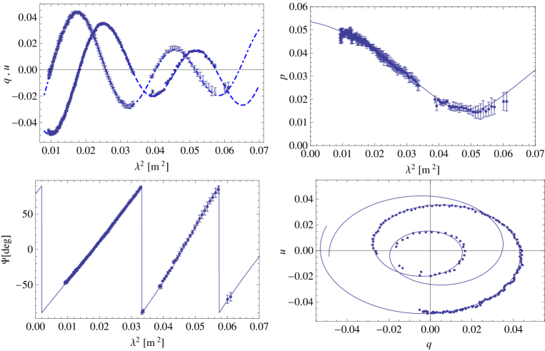
Figure 12: As for Figure 10 for PKS B160-771, but fitted with a two RM-component model.

A two RM-component model, shown in Figure 12, provides a much better description of the data as demonstrated by the corresponding $\chi^{2}_{\nu}$ value of 1.04. The fit accounts for both the changing slope of $\Psi(\lambda^{2})$ as well as the increasing $p(\lambda^{2})$ for $\lambda^{2}>0.05$ m². The best-fit RMs are $+107.1\pm 0.2$ rad m^-2 and $+78.7\pm 0.4$ rad m^-2 for the first and second component, respectively. The BIC strongly favours the two RM-component model over the depolarizing screen model (see Table 3 for values).

5.4 PKS B1039-47

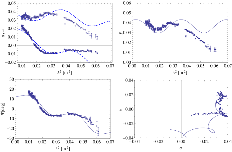
Figure 13: Polarisation data for PKS B1039-47, and the corresponding best-fit two RM-component model. Layout as described in Figure 4.

This is the most striking source in terms of complex polarization structure. Figure 13 shows how both $\Psi(\lambda^{2})$ and $p(\lambda^{2})$ display non-linear, oscillatory behaviour indicative of multiple RM components. The RMCLEAN spectrum also indicates the presence of multiple RM components (Fig. 3d).

We list a single RM-component model in Table 3 for completeness but do not show the fit. A two RM-component model (both components Faraday thin) also provides a poor description of the data (Fig. 13) with a reduced-$\chi^{2}$ value of 14, and this can be seen quite clearly in the $p(\lambda^{2})$ distribution. We then tried models with one Faraday thin and one Faraday thick component where the Faraday thick component was described by either Eqn. 9 or Eqn. 10. In both cases, neither model converged to an acceptable solution and they are not shown here.

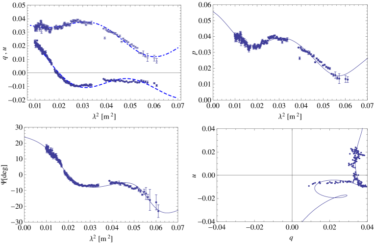
Figure 14: As for Figure 13 for PKS B1039-47, but fit by a three RM-component model (all Faraday thin).

Our next approach was to fit models with three RM components, which in the case of all Faraday thin components have a total of nine parameters (i.e. $p_{0}$, RM, & $\Psi_{0}$ for each component). In order to find a good model, we first fixed the parameters of the dominant RM component taken from RMCLEAN and let the other six model parameters vary. We then used these results as input guesses for the final nine parameter model fit. This returned best-fit RMs of $-13.1\pm 1.5$ rad m^-2, $-29.8\pm 2.4$ rad m^-2 and $+68.4\pm 1.6$ rad m^-2, listed in order of highest to lowest polarized fractions for the individual components. This provides a good fit, shown in Figure 14, with a $\chi^{2}_{\nu}$ value of 1.2 (Table 3).

We also tried different combinations of Faraday thin and thick components within a three RM-component model with the best model shown in Figure 15. Both the BIC and $\chi^{2}_{\nu}$ values are almost identical for both types of three-component model listed in Table 3, so they do not help us to clearly discriminate between models in this case. More data, at longer wavelengths, is required to determine which three-component model provides a better fit. A four-component model (all Faraday thin) was also tried but did not improve the fit.

6 Discussion

6.1 Physical origin of the RM components

We have conclusively shown in the previous section that for two sources (PKS B1610-771 & PKS B1039-47) we can spectrally resolve multiple polarized components of spatially unresolved AGN. We now discuss the likelihood of these additional RM components coming from regions of polarized emission along the line of sight or from multiple polarized regions on the plane of the sky but within our synthesised beam. Polarized diffuse Galactic emission (Testori et al., 2008) and polarized emission from radio halos/relics in galaxy clusters (e.g. Ferrari et al., 2008) are the most likely candidates for any additional polarized emission components along the line of sight. However, both these possibilities are highly unlikely for our particular observations since first, we do not have the sufficient short $uv$-spacings to detect the smooth Galactic emission and secondly, none of the sources studied here have any diffuse X-ray emission associated with them in the ROSAT All Sky Survey (RASS; Voges et al., 1999), which effectively rules out the presence of any significant emission from galaxy clusters along the line of sight.

If the sources were spatially unresolved, double-lobed radio galaxies such that our line of sight to one of the lobes travelled through a different magneto-ionic medium, then the polarized emission from each lobe would experience different amounts of Faraday rotation and could show up in our data as two distinct RM components (e.g. Slysh, 1965; Goldstein & Reed, 1984). For blazar type sources we require variation in the magneto-ionic medium along the jet because we only detect the Doppler boosted emission from the jet orientated toward us. Many high-resolution studies of such objects have shown substantial variations in both RM and polarized intensity on parsec-scales (e.g. Zavala & Taylor, 2003, 2004; O’Sullivan & Gabuzda, 2009; Hovatta et al., 2011). Below we discuss what is already known for each source and why the mostly likely origin of the additional RM components is from the compact inner regions of the radio source.

PKS B1903-802 is a flat spectrum radio quasar which, from 1.4 to 20 GHz, maintains a total flux density of $\sim$1 Jy while remaining polarized at $\sim$3% (Murphy et al., 2010). From 43 GHz observations with the ATCA, we know that this source is unresolved down to at least 0.15” (Rajan Chhetri, private communication) which corresponds to a linear scale of $\sim$0.9 kpc for the quoted redshift of this source (Table 1). The source is resolved into two total intensity components on scales less than 5 mas (30 pc) from observations at 8.4 GHz with the Australian Long Baseline Array (LBA; Ojha et al., 2005). No spectral index or polarization information is available on these scales but at least one of these components must be the origin of the strong polarized emission we see in our data. Hence, it is likely that there is a significant contribution to the observed RM from the immediate environment of the source and its host galaxy as well as the Faraday rotation caused by our own Galaxy.

PKS B0454-810 is a well studied flat spectrum radio quasar (e.g. Ricci et al., 2004) and has an inverted radio light curve which begins to turn over above 100 GHz (Bennett et al., 2003). Ricci et al. (2004) detected polarized emission of $\sim$2.6% at 18.5 GHz while Murphy et al. (2010) quote an upper limit of $1.5\%$ from 20 GHz ATCA observations. While it has been detected in X-rays (Voges et al., 1999), it does not have a $\gamma$-ray detection from Fermi (Abdo et al., 2009, 2011). It is spatially unresolved down to at least 5” ($\sim$30 kpc) from inspection of the visibilities on the longest baselines in our observations. It has also been imaged on milliarcsecond scales with both the VLBI Space Observatory Programme (Dodson et al., 2008) and the LBA (Ojha et al., 2005), showing that it is resolved on scales less than 5 mas. Rayner et al. (2000) found the source to be circularly polarized, with a $>10\sigma$ detection at both 1.4 and 5 GHz, which is indicative of a core-dominated AGN. Therefore, all this data supports our assertion that the linearly polarized emission we detect is coming from the compact inner regions of the AGN jet and provides some weight to our explanation for the observed variation in $p(\lambda^{2})$ being due to the combination of a weakly polarized optically-thick region and a strongly polarized optically-thin region.

PKS B1610-771 has been extensively studied across a wide range of wavelengths. It is classified as a flat-spectrum radio quasar (e.g. Healey et al., 2007), is significantly polarized (1–2% level) at 5, 8 and 20 GHz (Massardi et al., 2008) and is highly polarized ($>$3%) in the optical (Véron-Cetty & Véron, 2006). It is coincident with an unresolved X-ray source (Voges et al., 1999) and has a GeV $\gamma$-ray detection in both the first and second Fermi-LAT catalogues (Abdo et al., 2009, 2011). No source structure is detected on scales greater than 0.15” (Chhetri, private comm.), which corresponds to a linear scale of $\sim$1.3 kpc at its redshift of 1.71 (Hunstead & Murdoch, 1980). PKS B1610-771 is also seen to exhibit interstellar scintillation at low radio frequencies, with a characteristic time scale of 400 days (Gaensler & Hunstead, 2000). This further supports the conclusion that its flux is dominated by compact rather than extended components. On milliarcsecond scales at 8.4 GHz the jet extends in a North-West direction with several bright jet knots in total intensity seen out to a projected distance of $\sim$130 pc (Ojha et al., 2010). From our analysis of this source, we predict that two of these knots are strongly polarized and have different RMs.

PKS B1039-47 is classified as a flat-spectrum radio quasar that is located along a sightline $\sim$10^∘ from the Galactic plane, and has been measured to be $\sim$4% polarized at 20 GHz (Massardi et al., 2008). The host galaxy has a measured redshift of 2.59 (O. Titov, private communication) and there is no X-ray or $\gamma$-ray detection for this source. The emission structure remains unresolved down to 0.15” (1.2 kpc), and an LBA image from Ojha et al. (2004) shows a jet extending to the North-West out to $\sim$20 mas (160 pc), composed of three bright total intensity regions. Our analysis in this paper, which finds a best-fit three RM-component model for this source, suggests that each of these regions is polarized.

Therefore, in the case of PKS B1610-771 and PKS B1039-47, we claim to have detected separate polarized components in the compact inner regions of the jet on parsec-scales that are illuminating an inhomogeneous magneto-ionic medium in the immediate vicinity of the jet. The largest RM difference between different components that we have found from our model fits is $\sim$100 rad m^-2 (between the second and third components in PKS B1039-47). This is not inconsistent with recent measurements on milliarcsecond scales at 1.4 GHz where variations of 10s to 100s of rad m^-2 have been measured in several blazars (Coughlan et al., 2011). We can test our predictions for these sources through multi-frequency polarization sensitive observations with the LBA, which will allow us to spatially probe their milliarcsecond scale polarized structure for the first time.

6.2 RM time-variability

If we attribute the RM difference between components to the magneto-ionic material in the immediate vicinity of the parsec-scale jet then there are obvious implications for any observed time-variability from RM measurements on arcsecond scales and greater. The polarized and RM structure of VLBI jets has been observed to vary on timescales as short as months (e.g. Gómez et al., 2011; Zavala & Taylor, 2001), so the relative polarized flux of the individual components detected in our ATCA observations may also vary on similar timescales. Therefore, the relative difference between the individual component RM values may also vary if the polarized components are moving along the jet and illuminating different parts of an inhomogeneous Faraday screen close to the AGN. This means that RM time-variability for observations on similar angular scales to those presented in this paper may be simply due to the observations sampling different dominant RM components as they move along the jet or, if the observations do not have sufficient frequency coverage and spectral resolution, a complicated combination of multiple RM components that does not accurately represent any of the components.

Law et al. (2011) were able to compare four sources from their low spatial resolution, wide-bandwidth 1–2 GHz observations with high spatial resolution RM maps from the Very Long Baseline Array (VLBA). In general, they did not detect the high fractional polarization or high RM values seen from 5 to 22 GHz in the VLBA images. This is not surprising since the high spatial resolution of VLBA observations are less affected by beam depolarization and also because RMs on these scales have been observed to increase with increasing frequency (O’Sullivan & Gabuzda, 2009). Another possibility is that there may be intermediate scale polarized structure that the VLBA is not sensitive to, negating the validity of the comparison. Therefore, parsec-scale VLBI observations at similar frequency ranges taken as close in time as possible to the low spatial-resolution, wide-bandwidth observations are required for direct comparison. If the results from both these types of observations can be linked then it may be possible with multi-epoch polarization observations with wide-bandwidth facilities like the ATCA to map out the parsec-scale evolution of polarized components as well as the Faraday rotating environment in AGN jets, as suggested by Law et al. (2011).

Even though the majority of the Faraday rotation occurs as the polarized radiation passes through our Galaxy, the RM difference between multiple components as well as any observed variability is likely due to the magneto-ionic material in the immediate vicinity of the AGN jet. Hence, the type of sources studied in this paper may not be suitable as primary polarization calibrators since the values for their RMs and degree of polarization are likely to change on short timescales. A more stable type of calibrator source would be one in which the polarized emission comes from extended emission regions such as the lobes which vary on much longer timescales.

6.3 Reliability of RMCLEAN

For PKS B1903-802 the peak RM found using RMCLEAN agrees very well (within $\sim$0.3 rad m^-2) with the mean RM found from our best-fit external Faraday dispersion model. In the case of PKS B0454-810, the RM extracted using RMCLEAN differs by $\sim$2 rad m^-2 from what we consider to be the correct RM for this source. However, the comparison in this case is somewhat unreliable since we have not been able to conclusively identify the correct polarization model for this source.

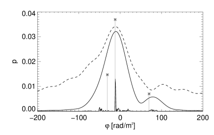
Figure 16: Simulated three component model without noise for PKS B1039-47 but with identical $\lambda^{2}$ coverage as in Figure 3(d). Stars: input model components taken from the best fit to PKS B1039-47 data shown in Figure 14. Dashed line: Dirty RM synthesis spectrum from simulated data. Solid line: RMclean spectrum from simulated data. Clean-component positions and amplitudes are also included on plot.

There have been some questions raised in the literature about the ability of the RMCLEAN method to accurately recover multiple RM components for sources with complex Faraday structure (e.g. Frick et al., 2010; Farnsworth et al., 2011). We find that the RMCLEAN method performs poorly in recovering the correct RMs for PKS B1610-771 and PKS B1039-47. While it does predict the presence of multiple RM components, the clean-component distribution does not match what is found through model-fitting $q(\lambda^{2})$, $u(\lambda^{2})$ (Fig. 3c,d). For PKS B1039-47, we investigated whether or not the three best-fit model RM components could be recovered with the same $\lambda^{2}$-coverage but with no noise. Figure 16 shows that again, after RMCLEAN, the clean-component distribution does not associate polarized power with the correct RM model-component locations. On reflection this may not be very surprising given that the RM resolution of our experiment is $\sim$60 rad m^-2 and is therefore unable to resolve multiple RM components which differ by less that this value. Thus, in cases of complex RM structure of extragalactic point sources, alternative reconstruction algorithms (e.g. Li et al., 2011) need to be investigated for application in all-sky RM surveys. Currently, the best approach for sources with complex Faraday depth structure is model-fitting multiple RM-component models to the observed $q(\lambda^{2})$ and $u(\lambda^{2})$ in order to find the most likely physical model for the source.

Table 3: Comparison between narrow-band and wide-band RMs

Source	RMwide	RM${}_{\rm old~{}ATCA}$	RMNVSS
	[rad m-2]	[rad m-2]	[rad m-2]
PKS B1903-802	$+18.1\pm 0.1$	$+18.2\pm 0.4$	$+21.5\pm 1.3$
PKS B0454-810	$+37.8\pm 0.2$	$+39.9\pm 1.2$	$+38.9\pm 1.5$
PKS B1610-771	$+107.1\pm 0.2$	$+134.6\pm 1.0$	$+128.5\pm 2.7$
PKS B1039-47	$-13.1\pm 1.5$	$-13.0\pm 6.7$	$-8.9\pm 1.2$

RM_wide: RM of main component derived from 1.1–3.1 GHz data. RM_narrow: RM derived using data from 1304–1494 MHz. RM_NVSS: derived using the same frequency coverage as in Taylor et al. (2009).

6.4 Some implications for RM surveys

Taking the same data but restricting the frequency range to 20 x 10 MHz channels, centred at 1.4 GHz, allowed us to compare the RMs derived from the full 2 GHz bandwidth with the previous narrow-band system on the ATCA (e.g. Feain et al., 2009). Using the fitting procedure employed throughout this paper, we find that we get the same RMs (within the errors) using 200 MHz of data for both PKS B1903-802 and PKS B0454-810. In this case, a single RM-component model with external Faraday dispersion still provides a better fit over a model without depolarization. In Table 3, for each source, we list the RM of the strongest polarized component derived from the full 1.1–3.1 GHz data to compare with the RM derived from the restricted range of 1.340–1.494 GHz.

For PKS B1610-771 we obtain a good fit ($\chi^{2}_{\nu}=1.2$, BIC$=-475$) for a single RM-component with external Faraday dispersion giving a mean RM of $+134.6\pm 1.0$ rad m^-2 and a dispersion of $10.9\pm 0.5$ rad m^-2. A marginally poorer fit is found using a two RM-component model ($\chi^{2}_{\nu}=1.3$, BIC$=-452$) with RM${}_{1}=+110.1\pm 1.8$ rad m^-2 and RM${}_{2}=+79.7\pm 2.1$ rad m^-2. Therefore, in this case we would adopt the single RM-component model since the evidence does not favour the more complex two RM-component model. But we already know that the two RM-component model is preferred using the full 2 GHz bandwidth data. The difference in RM between the single-component model and the strongest component in the two RM-component model is $\sim 25$ rad m^-2 (Table 3). This is quite a dramatic example of how wrong one can be in estimating the RM using narrow-bandwidth data. This highlights the important role wide-bandwidth data play in determining the correct Faraday depth structure of AGN on these angular scales. The best-ft model for PKS B1039-47 using the data from 1.340–1.494 GHz has two RM components where the strongest component has an RM equal (within the errors) to that found from the 1.1–3.1 GHz data.

Due to our small sample size we are unable to comment on how often additional RM components may be detected in extragalactic sources. From a sample of 37 bright, polarized sources Law et al. (2011) found that $\sim$25% of sources had an extra RM component detected with a significance greater than 7$\sigma$ ($\sim$40 mJy). They also found that the polarized flux weighted mean RM was similar to the low resolution RMs quoted by Taylor et al. (2009). This suggests that sources like PKS B1610-771 may be rare where the flux weighted mean RM ($\sim$97 rad m^-2) is significantly different from the RM which is derived from narrow-bandwidth observations. We also list in Table 3 the RMs calculated from our data using the same frequency setup as used by Taylor et al. (2009). For the simple sources, the RMs agree within 2–3 rad m^-2.

Current and upcoming spectropolarimetric all-sky RM surveys such as GALFACTS (Taylor & Salter, 2010) and the POSSUM survey on ASKAP (Gaensler et al., 2010) plan to extract RMs from observations with 300 MHz of instantaneous bandwidth near 1.4 GHz. For sources with a single RM-component modified by depolarization from external Faraday dispersion, observations with 300 MHz of bandwidth will produce the same results as we have found using 2 GHz of bandwidth (e.g. PKS B1903-802). In the case of sources with multiple RM components, it is strongly recommended that modelling of $q(\lambda^{2})$, $u(\lambda^{2})$ be undertaken instead of using the reconstruction algorithm RMCLEAN. Since ASKAP will have much better RFI conditions than at the ATCA, we use simulated data from the best-fit models for PKS B1610-771 and PKS B1039-47 (highlighted in bold in Table 3) instead of the observed data. Using the planned POSSUM frequency coverage of 1130–1430 GHz, we find that our modelling procedure would recover the correct two RM-component model for PKS B1610-771. For PKS B1039-47, depending on the quality of the data, it may be difficult to determine whether a two or three RM-component model provides the best fit. Complementary observations from a 300 MHz band at lower frequencies (e.g. 0.7–1.0 GHz) would enable us to recover the correct simulated three RM-component model in this case.

7 Conclusion

Using the new wide-bandwidth receivers on the ATCA, we have shown that we can spectrally resolve the polarization structure of spatially unresolved radio sources. We have identified two AGN (PKS B1610-771 and PKS B1039-47) where more than one rotation measure (RM) component is required to describe the Faraday structure of the source. We further demonstrate that modelling of both the polarization angle and degree of polarization dependences with wavelength squared is essential in determining the true Faraday depth structure of extragalactic point sources. We also find that the RM synthesis reconstruction algorithm RMCLEAN does not recover the correct RMs for sources with multiple RM components in our data.

The most likely origin for the additional RM components in both PKS B1610-771 and PKS B1039-47 is from the compact inner jet regions on parsec scales. This leads us to suggest that RM time-variability in extragalactic point sources may be due to the evolving polarized jet structure on parsec scales which illuminates different parts of an inhomogeneous magneto-ionic medium in the immediate vicinity of the jet. Follow-up observations of these particular sources with parsec-scale spatial resolution using the Australian Long Baseline Array (LBA) will enable us to test our predictions. Hence, with multi-epoch polarization observations using wide-bandwidth facilities like the ATCA it may be possible to map out the parsec-scale evolution of polarized components as well as the Faraday rotating environment in AGN jets.

In the near future, combining data from the pristine RFI environment of ASKAP from 0.7 to 1.8 GHz with data from the ATCA at higher frequencies can provide an exquisite probe of the polarization properties of a much larger sample of AGN.

Figure 2: Plots of the rotation measure spread function (RMSF). Solid line: RMSF from Jan 20. Dash-dot line: RMSF from Jan 9.

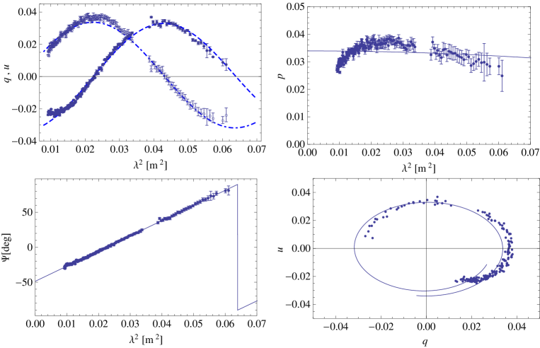
Figure 8: As for Figure 7 for PKS B0454-810, but fit by a single RM-component model with depolarization from external Faraday dispersion (Eqn. 11).

Figure 15: As for Figure 13 for PKS B1039-47, but fit by a three RM-component model (two Faraday thin, one Faraday thick: Eqn. 9).

8 Acknowledgements

The Australia Telescope Compact Array is part of the Australian Telescope, which is funded by the Commonwealth of Australia for operation as a National Facility managed by CSIRO. We would like to thank the engineers, technicians and staff at CSIRO’s Marsfield and Narrabri sites who were involved in the successful upgrade of the 20/13 cm receiver systems to take advantage of the 2 GHz correlator bandwidth available in CABB. B.M.G. and T.R. acknowledge the support of the Australian Research Council through grants DP0986386 and FS100100033, respectively. S.P.O’S. would like to thank David McConnell, Jamie Stevens, Mark Weiringa, Julie Banfield, Tim Cawthorne, Russell Jurek and Chris Hales for helpful discussions. This research has made use of NASA’s Astrophysics Data System Service and the NASA/IPAC Extragalactic Database (NED) which is operated by the Jet Propulsion Laboratory, California Institute of Technology, under contract with the National Aeronautics and Space Administration.

References

- Abdo et al. (2009) Abdo A. A., Ackermann M., Ajello M., Atwood W. B., Axelsson M., Baldini L., Ballet J., Barbiellini G., Bastieri D., Baughman B. M., Bechtol K., Bellazzini R., Blandford R. D., Bloom E. D., 2009, ApJ, 700, 597
- Abdo et al. (2011) Abdo A. A., Ackermann M., Ajello M., Atwood W. B., Axelsson M., Baldini L., Ballet J., Barbiellini G., Bastieri D., Baughman B. M., Bechtol K., Bellazzini R., Blandford R. D., Bloom E. D., 2011, ApJ, submitted, arXiv:1108.1420
- Beck & Gaensler (2004) Beck R., Gaensler B. M., 2004, New Astron. Rev., 48, 1289
- Bennett et al. (2003) Bennett C. L., Hill R. S., Hinshaw G., Nolta M. R., Odegard N., Page L., Spergel D. N., Weiland J. L., Wright E. L., Halpern M., Jarosik N., Kogut A., Limon M., Meyer S. S., Tucker G. S., Wollack E., 2003, ApJS, 148, 97
- Bonafede et al. (2010) Bonafede A., Feretti L., Murgia M., Govoni F., Giovannini G., Dallacasa D., Dolag K., Taylor G. B., 2010, A&A, 513, A30
- Brentjens & de Bruyn (2005) Brentjens M. A., de Bruyn A. G., 2005, A&A, 441, 1217
- Brown et al. (2007) Brown J. C., Haverkorn M., Gaensler B. M., Taylor A. R., Bizunok N. S., McClure-Griffiths N. M., Dickey J. M., Green A. J., 2007, ApJ, 663, 258
- Burn (1966) Burn B. J., 1966, MNRAS, 133, 67
- Coughlan et al. (2011) Coughlan C., Murphy R., Mc Enery K., Patrick H., Hallahan R., Gabuzda D., 2011, 10th EVN Symposium, arXiv:1101.5942
- Dodson et al. (2008) Dodson R., Fomalont E. B., Wiik K., Horiuchi S., Hirabayashi H., Edwards P. G., Murata Y., Asaki Y., Moellenbrock G. A., Scott W. K., Taylor A. R., Gurvits L. I., 2008, ApJS, 175, 314
- Farnsworth et al. (2011) Farnsworth D., Rudnick L., Brown S., 2011, AJ, 141, 191
- Feain et al. (2009) Feain I. J., Ekers R. D., Murphy T., Gaensler B. M., Macquart J.-P., Norris R. P., Cornwell T. J., Johnston-Hollitt M., Ott J., Middelberg E., 2009, ApJ, 707, 114
- Ferrari et al. (2008) Ferrari C., Govoni F., Schindler S., Bykov A. M., Rephaeli Y., 2008, Space Science Review, 134, 93
- Frick et al. (2010) Frick P., Sokoloff D., Stepanov R., Beck R., 2010, MNRAS, 401, L24
- Gaensler (2009) Gaensler B. M., 2009, in IAU Symposium Vol. 259 of IAU Symposium, Cosmic Magnetic Fields: From Planets, to Stars and Galaxies. pp 645–652
- Gaensler et al. (2005) Gaensler B. M., Haverkorn M., Staveley-Smith L., Dickey J. M., McClure-Griffiths N. M., Dickel J. R., Wolleben M., 2005, Science, 307, 1610
- Gaensler & Hunstead (2000) Gaensler B. M., Hunstead R. W., 2000, PASA, 17, 72
- Gaensler et al. (2010) Gaensler B. M., Landecker T. L., Taylor A. R., POSSUM Collaboration 2010, in BAAS Vol. 42. p. 470.13
- Goldstein & Reed (1984) Goldstein Jr. S. J., Reed J. A., 1984, ApJ, 283, 540
- Gómez et al. (2011) Gómez J. L., Roca-Sogorb M., Agudo I., Marscher A. P., Jorstad S. G., 2011, ApJ, 733, 11
- Harvey-Smith et al. (2011) Harvey-Smith L., Madsen G. J., Gaensler B. M., 2011, ApJ, 736, 83
- Heald et al. (2009) Heald G., Braun R., Edmonds R., 2009, A&A, 503, 409
- Healey et al. (2007) Healey S. E., Romani R. W., Taylor G. B., Sadler E. M., Ricci R., Murphy T., Ulvestad J. S., Winn J. N., 2007, ApJS, 171, 61
- Högbom (1974) Högbom J. A., 1974, A&AS, 15, 417
- Hovatta et al. (2011) Hovatta T., Lister M. L., Aller M. F., Aller H. D., Homan D. C., Kovalev Y. Y., Pushkarev A. B., Savolainen T., 2011, in Beamed and Unbeamed Gamma-rays from Galaxies. Journal of Physics: Conference Series, arXiv:1108.1514
- Hunstead & Murdoch (1980) Hunstead R. W., Murdoch H. S., 1980, MNRAS, 192, 31P
- Laing et al. (2008) Laing R. A., Bridle A. H., Parma P., Murgia M., 2008, MNRAS, 391, 521
- Law et al. (2011) Law C. J., Gaensler B. M., Bower G. C., Backer D. C., Bauermeister A., Croft S., Forster R., Gutierrez-Kraybill C., Harvey-Smith L., Heiles C., Hull C., Keating G., MacMahon D., Whysong D., Williams P. K. G., Wright M., 2011, ApJ, 728, 57
- Li et al. (2011) Li F., Brown S., Cornwell T. J., de Hoog F., 2011, A&A, 531, A126
- Mao et al. (2010) Mao S. A., Gaensler B. M., Haverkorn M., Zweibel E. G., Madsen G. J., McClure-Griffiths N. M., Shukurov A., Kronberg P. P., 2010, ApJ, 714, 1170
- Mao et al. (2008) Mao S. A., Gaensler B. M., Stanimirović S., Haverkorn M., McClure-Griffiths N. M., Staveley-Smith L., Dickey J. M., 2008, ApJ, 688, 1029
- Massardi et al. (2008) Massardi M., Ekers R. D., Murphy T., Ricci R., Sadler E. M., Burke S., de Zotti G., Edwards P. G., Hancock P. J., Jackson C. A., 2008, MNRAS, 384, 775
- Mauch et al. (2003) Mauch T., Murphy T., Buttery H. J., Curran J., Hunstead R. W., Piestrzynski B., Robertson J. G., Sadler E. M., 2003, MNRAS, 342, 1117
- Middelberg (2006) Middelberg E., 2006, PASA, 23, 64
- Murphy et al. (2010) Murphy T., Sadler E. M., Ekers R. D., Massardi M., Hancock P. J., Mahony E., Ricci R., Burke-Spolaor S., Calabretta M., Chhetri R., de Zotti G., 2010, MNRAS, 402, 2403
- Ojha et al. (2005) Ojha R., Fey A. L., Charlot P., Jauncey D. L., Johnston K. J., Reynolds J. E., Tzioumis A. K., Quick J. F. H., Nicolson G. D., Ellingsen S. P., McCulloch P. M., Koyama Y., 2005, AJ, 130, 2529
- Ojha et al. (2004) Ojha R., Fey A. L., Johnston K. J., Jauncey D. L., Reynolds J. E., Tzioumis A. K., Quick J. F. H., Nicolson G. D., Ellingsen S. P., Dodson R. G., McCulloch P. M., 2004, AJ, 127, 3609
- Ojha et al. (2010) Ojha R., Kadler M., Böck M., Booth R., Dutka M. S., Edwards P. G., Fey A. L., Fuhrmann L., Gaume R. A., Hase H., Horiuchi S., 2010, A&A, 519, A45
- O’Sullivan & Gabuzda (2009) O’Sullivan S. P., Gabuzda D. C., 2009, MNRAS, 393, 429
- Pizzo et al. (2011) Pizzo R. F., de Bruyn A. G., Bernardi G., Brentjens M. A., 2011, A&A, 525, A104
- Rayner et al. (2000) Rayner D. P., Norris R. P., Sault R. J., 2000, MNRAS, 319, 484
- Ricci et al. (2004) Ricci R., Sadler E. M., Ekers R. D., Staveley-Smith L., Wilson W. E., Kesteven M. J., Subrahmanyan R., Walker M. A., Jackson C. A., De Zotti G., 2004, MNRAS, 354, 305
- Rossetti et al. (2008) Rossetti A., Dallacasa D., Fanti C., Fanti R., Mack K.-H., 2008, A&A, 487, 865
- Sault et al. (1995) Sault R. J., Teuben P. J., Wright M. C. H., 1995, in R. A. Shaw, H. E. Payne, & J. J. E. Hayes ed., Astronomical Data Analysis Software and Systems IV Vol. 77 of ASP Conference Series. p. 433
- Schwarz (1978) Schwarz G., 1978, Ann. Statist., 6, 461
- Slysh (1965) Slysh V. I., 1965, AZh, 42, 689
- Sokoloff et al. (1998) Sokoloff D. D., Bykov A. A., Shukurov A., Berkhuijsen E. M., Beck R., Poezd A. D., 1998, MNRAS, 299, 189
- Stickel et al. (1994) Stickel M., Meisenheimer K., Kuehr H., 1994, A&AS, 105, 211
- Taylor & Salter (2010) Taylor A. R., Salter C. J., 2010, in R. Kothes, T. L. Landecker, & A. G. Willis ed., ASP Conference Series Vol. 438. p. 402
- Taylor et al. (2009) Taylor A. R., Stil J. M., Sunstrum C., 2009, ApJ, 702, 1230
- Testori et al. (2008) Testori J. C., Reich P., Reich W., 2008, A&A, 484, 733
- Tribble (1991) Tribble P. C., 1991, MNRAS, 250, 726
- Trotta (2008) Trotta R., 2008, Contemporary Physics, 49, 71
- Van Eck et al. (2011) Van Eck C. L., Brown J. C., Stil J. M., Rae K., Mao S. A., Gaensler B. M., Shukurov A., Taylor A. R., Haverkorn M., Kronberg P. P., McClure-Griffiths N. M., 2011, ApJS, 728, 97
- Véron-Cetty & Véron (2006) Véron-Cetty M.-P., Véron P., 2006, A&A, 455, 773
- Voges et al. (1999) Voges W., Aschenbach B., Boller T., Bräuninger H., Briel U., Burkert W., Dennerl K., Englhauser J., Gruber R., Haberl F., Hartner G., Hasinger G., 1999, A&A, 349, 389
- Wilson et al. (2011) Wilson W. E., Ferris R. H., Axtens P., Brown A., Davis E., Hampson G., Leach M., Roberts P., Saunders S., 2011, MNRAS, 416, 832
- Zavala & Taylor (2001) Zavala R. T., Taylor G. B., 2001, ApJ, 550, 147
- Zavala & Taylor (2003) Zavala R. T., Taylor G. B., 2003, ApJ, 589, 126
- Zavala & Taylor (2004) Zavala R. T., Taylor G. B., 2004, ApJ, 612, 749