Distributed Soft Coding with a Soft Input Soft Output (SISO) Relay Encoder in Parallel Relay Channels

Abstract

In this paper, we propose a new distributed coding structure with a soft input soft output (SISO) relay encoder for error-prone parallel relay channels. We refer to it as the distributed soft coding (DISC). In the proposed scheme, each relay first uses the received noisy signals to calculate the soft bit estimate (SBE) of the source symbols. A simple SISO encoder is developed to encode the SBEs of source symbols based on a constituent code generator matrix. The SISO encoder outputs at different relays are then forwarded to the destination and form a distributed codeword. The performance of the proposed scheme is analyzed. It is shown that its performance is determined by the generator sequence weight (GSW) of the relay constituent codes, where the GSW of a constituent code is defined as the number of ones in its generator sequence. A new coding design criterion for optimally assigning the constituent codes to all the relays is proposed based on the analysis. Results show that the proposed DISC can effectively circumvent the error propagation due to the decoding errors in the conventional detect and forward (DF) with relay re-encoding and bring considerable coding gains, compared to the conventional soft information relaying.

I Introduction

In wireless networks, the transmitted signal is overheard by all nodes in the vicinity of the transmitter. Similarly, a receiver can hear transmissions from multiple neighbouring nodes. This broadcast nature of wireless networks provides unique opportunities for collaborative and distributed signal processing techniques. Nodes other than the intended destination can listen to a signal at no additional transmission cost and it is globally efficient for these nodes to forward the information to the destination. This process of transmitting data from source to destination via one or more nodes is referred to as relaying, which has been shown to yield spatial diversity and great power savings [1-2].

Two most frequently used relaying protocols in relay networks are amplify and forward (AF) and detect and forward (DF), which is also referred to as the decode and forward for the coded systems [1-3, 37]. Recently, some variations of AF and DF protocols have been proposed to further improve the performance of relayed transmission, such as selective DF [1], soft information relaying (SIR) and adaptive relaying protocol (ARP) [9, 43, 45]. Among them, the SIR scheme has recently attracted a lot of interest due to its superior performance [4-8, 23-28, 33]. There are generally various ways to represent the soft information. Two commonly used SIR schemes are the SIR scheme based on soft bit estimate (SIR-SBE) and the SIR based on log-likelihood ratio (SIR-LLR).

The SIR-SBE schemes and soft encoding were first proposed in [4, 8], where a soft encoding method was developed to calculate the SBE of coded symbols. The SIR-LLR was first discussed in [5], where the relay calculates and forwards the LLR of received symbols. It was shown in [6, 31] that the SIR-SBE is an optimal relaying protocol in terms of minimizing the mean square error (MSE) or maximizing the overall destination SNR. The Gaussian distribution has been used to approximate the probability distribution function (PDF) of both SBE and LLR. However, it was later shown in [7, 29, 34] that the SBE of an encoder output does not follow the exact Gaussian distributions, which is particularly true for recursive encoders. To further improve the performance of SIR scheme, [29] proposed an accurate error model of SBE by dividing the error pattern in SBE into hard and soft errors and calculating them separately. It is shown that such error model is more accurate than the Gaussian distribution and brings considerable performance improvement. Soft fading was proposed in [36] as an alternative way to model the soft-errors introduced in SIR processing at the relay via fading coefficients. A mutual information based SIR scheme was developed in [33], where the relay forwarding function consists of the hard decisions of the symbol estimates and a reliability measure. The reliability measure was determined by the symbol-wise mutual information computed from the absolute value of the LLR at the relay. In [24], a novel approach was proposed for analyzing the performance of SIR scheme by calculating the mutual information loss due to the use of a soft channel encoder at the relay. Soft information estimate and forward scheme was further extended to higher order such as MQAM modulations in [28] and to two way relay networks in [26]. In general, all these schemes take advantage of soft information processing at the relay to improve system performance.

It is well known that the main performance degradation in a DF protocol is caused by the error propagation during the decoding and relay encoding process when decoding errors occur at the relay. Unlike DF protocol that makes a hard decision based on the transmitted information symbols at the relay, SIR can effectively alleviate error propagation by calculating and forwarding the corresponding soft information. Forwarding soft information at the relays provides additional information to the destination decoder to make decisions, instead of making premature decisions at the relay decoder. Thus SIR outperforms both AF and DF protocols and can achieve a full diversity order in fading channels [33].

Recently, some distributed coding schemes have been proposed to exploit the spatial diversity and the distributed coding gains in wireless relay networks [47]. By applying the space time coding principle, distributed space time codes [10-13, 49] have been proposed for wireless relay networks. To further improve the system performance, the distributed low density parity check (LDPC) codes [14, 15, 18], distributed turbo coding (DTC) [16, 17, 42, 44, 46, 48], irregular distributed space-time code [49] and distributed rateless coding [39-41] have been developed for a 2-hop single relay network. However, these distributed coding schemes are based on the DF relaying protocols and assume that either relays can always decode correctly or relays will not forward when they cannot decode correctly. Few of them have actually considered how to perform relay encoding when there are decoding errors in the source to relay links. In [29, 37], a few error models have been proposed for distributed coding using DF protocol by taking into account the decoding errors in the destination decoding. In [4, 7, 8, 23, 29, 31, 36, 38], distributed schemes with soft information encoding have been developed for a relaying system containing only one relay when imperfect decoding occurs at the relay. In these schemes, instead of making decisions on the transmitted information symbols at the relay as in other distributed coding schemes [14-18], the relay calculates and forwards the corresponding soft estimates. The soft information encoding methods proposed in these papers are basically a probability inference method developed for the convolutional codes. The encoding process is complicated and also it only considered one relay. Very recently soft encoding was applied to distributed turbo product and distributed LDPC codes in [35, 36]. It has been shown in these papers that the soft information encoding can effectively mitigate error propagation caused by the imperfect decoding and thus improve the system performance.

To facilitate the hardware implementation, in [23] Winkelbauer and Matz proposed a soft encoder structure implemented using shift registers based on the boxplus operation. It has greatly reduced the complexity of the soft encoder compared to the existing algorithms. However, the boxplus representation in the soft encoder are still quite complex and thus hard for performance analysis. Thus [23] only considered a single relay system, and no performance analysis and code design has been done. How to extend the soft encoding to general multiple parallel relay network and design the optimal codes for relay soft encoding remains an open problem.

Till now it is still unknown what is the optimal way to encode the noisy estimates of the source symbols to circumvent error propagation in the encoding process at the relay and simultaneously provide significant distributed coding gains in general multiple parallel relay network. It is still unclear if encoding these noisy estimates can bring any further gains. A general framework for designing and analyzing distributed coding in a general error-prone relay channel is needed.

In this paper, we propose a simple distributed coding scheme with soft input soft output (SISO) relay encoders for a two-hop parallel relay network with one source, multiple parallel relays and one destination. We refer to the proposed scheme as the distributed soft coding (DISC). In DISC, different relays exploit a SISO encoder to encode the received analog signals using different constituent codes. The proposed SISO relay encoder has a very simple encoding structure and can be implemented by using the structure of conventional channel encoders in the complex number domain. Compared to the SISO encoding scheme in [8], which is a probability inference method and involves complicated calculations in encoding process, the proposed SISO relay encoder can achieve the exactly the same performance, but has a very simple encoding structure. It performs the encoding of the noisy source symbol estimates at the relays. Each relay first calculates the SBEs of the source symbols and the SBEs are subsequently encoded by using the proposed SISO encoder, whose outputs are then forwarded to the destination. At the destination, the signals forwarded from various relays form a distributed codeword.

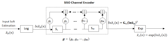
Figure 1: SISO channel encoder, where the addition is done in the complex field.

The performance of the DISC is then analyzed. It is shown that its performance is determined by the generator sequence weights (GSWs) of the relay constituent codes, where the GSW of a constituent code is defined as the number of ones in its generator sequence. To optimize the BER performance, one should make the GSW of each constituent code as large as possible by increasing the memory length of the relay encoder. This is the same as for the conventional convolutional codes. However, the GSWs cannot be chosen arbitrarily, as the code may become catastrophic for certain combinations of GSW values. For most of conventional noncatastrophic convolutional codes, GSWs are different for different constituent codes. Given K GSWs of K constituent codes, we need to determine what is the optimal way of pairing off the K constituent codes with K relays. A coding design criterion is proposed based on the BER performance analysis of the DISC. It is shown that for the optimal pairing one should match the GSW value of a constituent code to the corresponding input SNRs of a relay and assign the constituent code with a large GSW to the relay with a large input SNR. Simulation results show that the proposed DISC with optimal pairing is superior to the DISC with the un-ordered pairing. It is also shown that the DISC can effectively overcome error propagation in the encoding process at the relays and thus significantly outperforms the conventional detect and forward (DF) schemes with relay re-encoding. Furthermore, unlike the DF scheme, where the error performance degrades as the number of encoder states increases, the performance of the proposed DISC greatly improves as the number of encoder states increases thus bringing significant distributed coding gains compared to the conventional soft information relaying (SIR) without relay encoding.

The rest of the paper is organized as follows. In Section II, we describe the proposed DISC scheme. Its performance is analyzed in Section III. Section IV provides the simulation results. Conclusions are drawn in Section V.

Notations: In this paper, we use a lowercase and capital bold face letter to denote a vector and a matrix, respectively. The modulated signal of a symbol $b(n)$ is denoted as $x_{b}(n)$ and the soft estimate of $b(n)$, given its a posteriori probability, is denoted as $\tilde{x}_{b}(n)$.

II Distributed Soft Coding with a SISO Relay Encoder

In this section, we first briefly describe a SISO encoder using a single constituent convolutional code (CC) of rate 1. We then apply it to a general two-hop relay network using multiple constituent codes.

II-A SISO Convolutional Encoder

Let us consider a rate-1 CC with the generator sequence of $\mathbf{g}=(g_{1},g_{2},\ldots,g_{M})$ and the generator matrix $\mathbf{G}$. Let us denote by ${\bf{c}}=(c(1),\cdots,c(N))$ the encoder output codeword of information bits $\mathbf{b}=(b(1),\cdots,b(N))$, generated by the generator matrix $\mathbf{G}$, where $c(n)$ is the $n$-th code symbol of $\mathbf{b}$. Let ${{\bf{x}}_{c}}=\left({{x_{c}}(1),{x_{c}}(2),\cdots,{x_{c}}(N)}\right)$ represent the modulated sequence of $\mathbf{c}$.

Let $\mathbf{r}$ be a vector of analog signals, carrying information bits $\mathbf{b}$. Let us denote the a posteriori probability (APP) vector of $\mathbf{b}$, given $\mathbf{r}$, by

$${\bf{P}}{{\bf{r}}_{\bf{r}}}=\left\{{\left({{{Pr}_{0}}(1),{{Pr}_{1}}(1)}\right),\cdots,\left({{{Pr}_{0}}(N),{{Pr}_{1}}(N)}\right)}\right\},$$ (1)

where $Pr_{0}(n)$ and $Pr_{1}(n)$ are the APPs of $b(n)=0$ and $b(n)=1$, given $\mathbf{r}$ at time $n$. Given the APPs of $\mathbf{b}$, the soft bit estimate (SBE) of $b(n)$, denoted by ${\tilde{x}_{b}}(n)$, representing the expected value of ${x_{b}}(n)$, can be calculated as

$${\tilde{x}_{b}}(n)=E({x_{b}}(n)|{\bf{r}})={Pr_{0}}(n)-{Pr_{1}}(n).$$ (2)

As shown in [6, 8, 21], the SBE of symbol ${x_{b}}(n)$, denoted by ${\tilde{x}_{b}}(n)$, can be represented by the following model

$${\tilde{x}_{b}}(n)={x_{b}}(n)\left({1-{{\tilde{w}}}(n)}\right)=\alpha{x_{b}}(n)+{w_{in}}(n),$$ (3)

where ${w_{in}}(n)=-{x_{b}}(n)\left({{{\tilde{w}}}(n)-{\mu_{\tilde{w}}}}\right)$ is the noise term in the SBE with a zero mean and variance of $\sigma_{in}^{2}$, ${\tilde{w}}(n)>0$ is an equivalent noise independent of ${x_{b}}(n)$ with a mean

$${\mu_{\tilde{w}}}=\frac{1}{N}\sum_{n=1}^{N}{{\tilde{w}}(n)}=\frac{1}{N}\sum_{n=1}^{N}{(1-{x_{b}}(n){\tilde{x}_{b}}(n))},$$

and variance of

$$\sigma_{\tilde{w}}^{2}=\frac{1}{N}\sum_{n=1}^{N}{((1-{x_{b}}(n){\tilde{x}_{b}}(n)-\mu_{\tilde{w}}))^{2}},$$ (4)

and $\alpha=1-{\mu_{\tilde{w}}}$. It can be easily verified that ${x_{b}}(n)$ and ${w_{in}}(n)$ are independent.

Given $\mathbf{r}$, or equivalently, given the SBEs of information bits $\mathbf{b}$, now let us look at how to calculate the SBEs of the codeword $c(n)$ of $\mathbf{b}$, denoted by ${\tilde{x}_{c}}(n)$.

To calculate the SBEs of the codeword $\mathbf{c}$, let us first use the probability inference method in [8] to calculate the probabilities of $\mathbf{c}$, denoted by $Pr\left({{x_{c}}(n)|{{\bf{Pr_{r}}}}}\right)$, as follows

$$Pr\left({{x_{c}}(n)=q|{{\bf{Pr_{r}}}}}\right)=\sum\limits_{m\in U({x_{c}}(n)=q)}{{{Pr}_{{b_{c}}}}\left(n\right)Pr\left({{S_{m}}(n)}\right)}$$ (5)

$$Pr\left({{S_{m}}(n+1)}\right) = \sum\limits_{m^{\prime}}{Pr\left({{S_{m}}(n+1)|{S_{m^{\prime}}}(n)}\right)Pr\left({{S_{m^{\prime}}}(n)}\right)}$$ (6)

$$= \sum\limits_{m^{\prime}}{{{Pr}_{{b_{n}}(m,m^{\prime})}}\left(n\right)Pr\left({{S_{m^{\prime}}}(n)}\right)}$$

where $S_{m}(n)$ represents the encoder states of $m$ at time $n$, $U({x_{c}}(n)=q)$ is the set of branches, whose encoder output is equal to $q$, $b_{c}$ is the corresponding input information bit, ${Pr_{{b_{c}}}}\left(n\right)$ is the probability of $b_{c}$ at time $n$, ${b_{n}}(m,m^{\prime})$ represents the input information bit resulting in the transition from state $m^{\prime}$ at time $n$ to $m$ at time $n+1$, and ${Pr_{{b_{n}}(m,m^{\prime})}}\left(n\right)$ is the probability of information bit ${b_{n}}(m,m^{\prime})$ at time $n$.

To gain more insights into the soft encoding process, let us first consider a simple rate-1 CC with the generator sequence of $\mathbf{g}=(1,~{}1,~{}1)$ and apply the above equations alternatively to this code, we can easily find that the SBE of encoder input and output for this code has the following simple relationship

$${\tilde{x}_{c}}(n)={\tilde{x}_{b}}(n){\tilde{x}_{b}}(n-1){\tilde{x}_{b}}(n-2)$$ (7)

Let us define ${\bf{ln}}{{\bf{\tilde{x}}}_{b}}=\left({\ln{{\tilde{x}}_{b}}(1),\cdots,\ln{{\tilde{x}}_{b}}(N)}\right)$ and ${\bf{ln}}{{\bf{\tilde{x}}}_{c}}=\left({\ln{{\tilde{x}}_{c}}(1),\cdots,\ln{{\tilde{x}}_{c}}(N)}\right)$, where for a complex number $x=r{e^{j\theta}}$, $\ln x=\ln|r|+j\theta$. Therefore, for a negative real number $x<0$, $\ln x=\ln|x|+j\pi$. Then Eq. (7) can be further written as

$$\ln{\tilde{x}_{c}}(n) = \ln{\tilde{x}_{b}}(n)+\ln{\tilde{x}_{b}}(n-1)+\ln{\tilde{x}_{b}}(n-2)$$ (8)

$$= {{\bf{G}}_{n}}\left({{\bf{ln}}{{{\bf{\tilde{x}}}}_{b}}}\right)^{T}$$

$${\bf{ln}}{{\bf{\tilde{x}}}_{c}}=\mathbf{G}{\left({{\bf{ln}}{{{\bf{\tilde{x}}}}_{b}}}\right)^{T}}$$ (9)

where ${{\bf{G}}_{n}}$ is the $n$-th row of $\mathbf{G}$.

(8) and (9) are derived for an example constituent convolutional code (CC), but they can be applied to the general non-recursive convolutional codes, as shown in the following theorem.

Theorem 1 - SISO Encoder: Let ${\tilde{x}_{b}}\left(n\right)$ represent the input soft bit estimate (SBE) to a channel encoder. Then given a generator matrix ${\bf{G}}={\left({{\bf{G}^{T}_{1}},{\bf{G}^{T}_{2}},\cdots,{\bf{G}^{T}_{N}}}\right)^{T}}$ of a rate-1 linear constituent code, where ${\bf{G}}_{n}$ is the $n$-th row of G and the $ij$-th element of $\mathbf{G}$ is denoted by ${G_{ij}}$, ${G_{ij}}\in\left\{{0,1}\right\}$, the logarithm of the SISO encoder outputs for the soft inputs ${\bf{ln}}{{\bf{\tilde{x}}}_{b}}$, denoted by ${\bf{ln}}{{\bf{\tilde{x}}}_{c}}$, can be calculated as

$${\bf{ln}}{{\bf{\tilde{x}}}_{c}}={\bf{G}}{\left({{\bf{ln}}{{{\bf{\tilde{x}}}}_{b}}}\right)^{T}}.$$ (10)

The corresponding soft encoder outputs are given by

$${\tilde{x}_{c}}(n) = \exp\left({\ln{{\tilde{x}}_{c}}(n)}\right)=\exp\left({{{\bf{G}}_{n}}{{\left({{\bf{ln}}{{{\bf{\tilde{x}}}}_{b}}}\right)}^{T}}}\right)$$ (11)

$$= \exp\left({\sum\limits_{i=1}^{N}{{G_{ni}}\ln{{\tilde{x}}_{b}}(i)}}\right)=\prod\limits_{i\in\{{U_{n}}\}}{{{\tilde{x}}_{b}}(i)}$$

where ${U_{n}}=\{G_{nj}=1,j=1,...,N\}$, $n=1,...,N$, is the set of non-zero coefficients in ${\bf{G}}_{n}=({G_{n1}},{G_{n2}},\cdots,{G_{nN}})$.

Proof: See Appendix A.

Theorem 1 formulates a simple SISO encoder structure, which is shown in Fig. 1. As shown in the figure, the SISO encoder can be implemented by using a convolutional encoder structure, but the difference is that the addition operation in the SISO convolutional encoder is done in a complex field, not in binary field. We can see from the figure that the SISO channel encoder can be implemented by adding a logarithm and an exponential module at the front and the back of the conventional encoder, respectively.

II-B Distributed Soft Coding with a SISO Relay Encoder

In this subsection, we introduce a distributed soft coding (DISC) scheme for a general 2-hop parallel relay network based on the previously described SISO encoder. For simplicity, in the following sections, we consider a non-recursive convolutional code (NRCC) as the constituent code in the SISO encoder at each relay. As shown in Fig. 2, the network consists of one source, $K$ relays and one destination. We assume that there is no direct link between the source and destination as it is too weak compared to the relay links and is thus ignored. For simplicity, we assume that no channel coding is performed at the source node. Since we consider an uncoded system, we will refer to DF as the detect and forward in the rest of this paper. The proposed scheme can also be applied to the coded system. If a channel code is applied at the source, relays will perform the same soft encoding process as for an uncoded system, but a concatenated code will be formed at the destination.

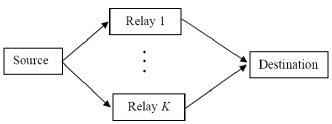
Figure 2: A general two-hop parallel relay network.

Let $\mathbf{b}=(b(1),\cdots,b(n),\cdots,b(N))$ be a binary information sequence of length $N$, generated by the source node. $\mathbf{b}$ is first modulated into a signal sequence $\mathbf{x_{b}}=(x_{b}(1),\cdots,x_{b}(n),\cdots,x_{b}(N))$ and then transmitted, where $x_{b}(n)$ is a modulated signal of $b(n)$. For simplicity, in this paper, we consider the BPSK modulation and assume that the symbol 0 and 1 are modulated into 1 and -1, respectively. Similar to [1, 2, 8, 9], we assume that the source and relays transmit signals over orthogonal channels. We will concentrate on a time division scheme, for which each node transmits in a separate time slot. The source first broadcasts the signals $\mathbf{x_{b}}$ to all $K$ parallel relays. Let ${{\bf{r}}_{s{r_{k}}}}=\left({r_{s{r_{k}}}(1),\cdots,r_{s{r_{k}}}(N)}\right)$ be the signals received at relay $k$, where

$$r_{s{r_{k}}}(n)=\sqrt{{P_{s{r_{k}}}}}h_{s{r_{k}}}{x_{b}}(n)+\eta_{{r_{k}}}(n),$$ (12)

${P_{s{r_{k}}}}={P_{s}}{L_{s{r_{k}}}}$ is the average power received at relay $k$, $P_{s}$ is the source transmit power, $L_{s{r_{k}}}$ and $h_{s{r_{k}}}$ are the pathloss and channel gain between the source and relay $k$, and $\eta_{{r_{k}}}(n)$ is a zero mean complex Gaussian noise with variance of $\sigma_{n}^{2}$.

Let ${\bf{g}}^{(k)}$ and $\mathbf{G}^{(k)}$ represent the generator sequence and generator matrix for relay $k$. $d_{k}$ denotes the number of ones in ${\bf{g}}^{(k)}$ and is referred to as the row degree of $\mathbf{G}^{(k)}$. Let ${{\bf{c}}_{k}}=({c_{k}}(1),\cdots,{c_{k}}(N))$ be the codeword of information bits b generated by $\mathbf{G}^{(k)}$, where $c_{k}(n)$ is the $n$-th code symbol of b. Let ${{\bf{x}}_{{c_{k}}}}=\left({{x_{{c_{k}}}}(1),{x_{{c_{k}}}}(2),\cdots,{x_{{c_{k}}}}(N)}\right)$ represent the modulated sequence of $\mathbf{c}_{k}$.

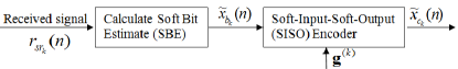
Figure 3: The encoder structure at relay k in DISC.

Fig. 3 shows the proposed encoder structure at relay $k$. In the proposed DISC scheme, each relay exploits a rate-1 SISO encoder to encode the received analog signals based on its assigned constituent code. It has been shown in [6] and [31] that the soft bit estimate of source information symbol is the optimal input to the soft encoder in terms of maximizing the SNR of the SISO encoder output. Thus upon receiving signals, relay $k$ first calculates the SBE of the source information symbol, denoted by ${\tilde{x}_{{b_{k}}}}(n)$. The relay $k$ then applies the SISO encoder described in Theorem 1 to encode ${\tilde{x}_{{b_{k}}}}(n)$, based on the given generator sequence ${\bf{g}}^{(k)}$, to generate the SBEs of its code sequence ${{\bf{c}}_{k}}$. Let $\tilde{x}_{{c_{k}}}(n)$ be the corresponding soft encoder output at relay $k$ at time $n$. By substituting (3) into (11), $\tilde{x}_{{c_{k}}}(n)$ can be expressed as

$$\tilde{x}_{{c_{k}}}(n) = \prod\limits_{j\in\{{U^{(k)}_{n}}\}}{{{\tilde{x}}_{b_{k}}}(j)}$$

$$= \prod\limits_{j\in\{{U^{(k)}_{n}}\}}{\left({\alpha_{k}{x_{b}}(j)+{w_{in,k}}(j)}\right)}$$

$$= {\alpha_{k}}^{{d_{k}}}{\prod\limits_{j\in\{{U^{(k)}_{n}}\}}{x_{b}}(j)}+{w_{out,k}}(n)$$

$$= {\alpha_{k}}^{{d_{k}}}{x_{{c_{k}}}}(n)+{w_{out,k}}(n),$$

where ${U^{(k)}_{n}}=\{G^{(k)}_{nj}=1,j=1,...,N\}$, $n=1,...,N$, is the set of non-zero coefficients in ${\bf{G}}^{(k)}_{n}=({G^{(k)}_{n1}},{G^{(k)}_{n2}},\cdots,{G^{(k)}_{nN}})$; ${x_{c_{k}}}(n)=\prod\limits_{j\in\{{U^{(k)}_{n}}\}}{{x_{b}}(j)}$ is the modulated signal of $n$-th code bit $c_{k}(n)$ of $\mathbf{b}$; ${\alpha_{k}}=1-{\mu_{\tilde{w},k}}$; $\mu_{\tilde{w},k}$ is the mean of equivalent noise ${\tilde{w}}(n)$ in the SBE at relay $k$ shown in (3), and ${w_{out,k}}(n)$ is the equivalent noise at the soft encoder output with a zero mean and variance of

$$\sigma_{out,k}^{2}={\left({\alpha_{k}^{2}+\sigma_{in,k}^{2}}\right)^{{d_{k}}}}-\alpha_{k}^{2{d_{k}}},$$ (14)

$\sigma_{in,k}^{2}$ is the variance of the equivalent noise ${w_{in}}(n)$ in the soft input to the SISO encoder of relay $k$, as shown in (3).

For simplicity, we assume that all relays transmit at the same power $P_{r}$. Then the signals transmitted from relay $k$ can then be written as

$$x_{{r_{k}}}(n)={\beta_{k}}\tilde{x}_{{c_{k}}}(n),$$ (15)

where ${\beta_{k}}$ is a normalization factor, given by

$$\beta_{k}=\sqrt{{P_{r}}/{P_{{x_{k}}}}},$$ (16)

where ${P_{{x_{k}}}}=E\left({{{\left|{\tilde{x}_{{c_{k}}}(n)}\right|}^{2}}}\right)={\left({\alpha_{k}^{2}+\sigma_{in,k}^{2}}\right)^{{d_{k}}}}$.

The destination received signal, transmitted from relay $k$, can be written as

$$y_{{r_{k}}d}(n)=\sqrt{{L_{r}}}h_{{r_{k}}d}x_{{r_{k}}}(n)+w_{{r_{k}}d}(n)~{}~{}~{}~{}~{}~{}~{}~{}~{}~{}~{}~{}~{}~{}~{}~{}~{}$$

$$=\sqrt{{L_{r}}}h_{{r_{k}d}}{\beta_{k}}\left({\alpha_{k}^{{d_{k}}}{{\tilde{x}}_{{c_{k}}}}(n)+{w_{out,k}}(n)}\right)+w_{{r_{k}}d}(n)$$

$$=\sqrt{{L_{r}}}h_{{r_{k}}d}{\beta_{k}}\alpha_{k}^{{d_{k}}}{\tilde{x}_{{c_{k}}}}(n)+\tilde{w}_{{r_{k}}d}(n),~{}~{}~{}~{}~{}~{}~{}~{}~{}~{}~{}~{}~{}~{}~{}~{}~{}~{}$$ (17)

where $L_{r}$ is the pathloss from the relay to the destination, $\tilde{w}_{{r_{k}}d}(n)=\sqrt{{L_{r}}}h_{{r_{k}}d}{\beta_{k}}{w_{out,k}}(n)+w_{{r_{k}}d}(n)$ is an equivalent noise with a zero mean and variance of

$$\sigma_{{r_{k}}d}^{2}=\sigma_{n}^{2}+L_{r}{\left|{h_{{r_{k}}d}}\right|^{2}}\beta_{k}^{2}\left[{{{\left({\alpha_{k}^{2}+\sigma_{in,k}^{2}}\right)}^{{d_{k}}}}-\alpha_{k}^{2{d_{k}}}}\right].$$ (18)

In the above equation, we have used the fact that $E\left({{w_{in,i}}(n){w_{in,j}}(n)}\right)=0$ for the BPSK constellation [6] and thus $E\left({{w_{out,i}}(n){w_{out,j}}(n)}\right)=0$.

As shown in [7][34], the noise term in the SBE $\omega_{in}(n)$ does not follow the exact Gaussian distribution, so does the equivalent noise of the soft encoder output $\omega_{out}(n)$ and the overall destination noise $\tilde{\omega}_{r_{k}d}(n)$. Fig. 4 plots the probability distribution function (PDF) of overall destination noise for the rate-1 4-state SISO encoder at various SNRs, which is also the conditional PDF of $Pr(y_{{r_{k}}d}(n)|{x_{c_{k}}}(n))$. The PDF curves are obtained by averaging over 1000 frames, each of which consists of 130 symbols. It can be seen from the figure that the overall destination noise can be roughly approximated by Gaussian distributions with some approximation errors. To simplify the decoding process and analysis, throughout the paper we assume that the overall destination noise follows the Gaussian distribution. Therefore, the conventional BCJR MAP decoding algorithm [32] can be directly applied to decode the destination received signals by treating the overall received signals as a codeword of rate $1/K$.

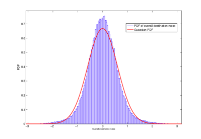
(a) $\bar{\gamma}_{s{r_{1}}}=\bar{\gamma}_{s{r_{2}}}=\bar{\gamma}_{rd}=6dB$;

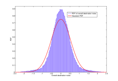
(b) $\bar{\gamma}_{s{r_{1}}}=\bar{\gamma}_{s{r_{2}}}=\bar{\gamma}_{rd}=8dB$;

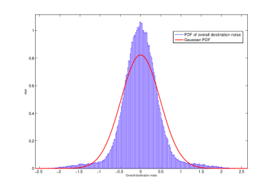
(c) $\bar{\gamma}_{s{r_{1}}}=\bar{\gamma}_{s{r_{2}}}=\bar{\gamma}_{rd}=10dB$;

Figure 4: PDF of overall destination noise for the 4-state SISO encoder.

III Performance Analysis and DISC Design

The SISO encoding at the relays can bring system some coding gains, but on the other hand soft encoding of noisy SBE will enhance the noise power at the destination, as shown in (II-B). It is unclear whether the coding gain can surpass the noise enhancement in the DISC and if such encoding can bring any overall gain. Moreover, given $K$ constituent codes, we need to determine what is the optimal way of pairing off the $K$ constituent codes with $K$ relays. In this section, we will give a quantitative analysis of the DISC scheme performance based on which a coding design criterion is then proposed.

By substituting (16) into (18), the variance of the equivalent destination noise in Eq. (18) can be expanded as

$$\sigma_{{r_{k}}d}^{2}=\sigma_{n}^{2}+L_{r}{\left|{h_{{r_{k}}d}}\right|^{2}}\beta_{k}^{2}\left[{{{\left({\alpha_{k}^{2}+\sigma_{in,k}^{2}}\right)}^{{d_{k}}}}-\alpha_{k}^{2{d_{k}}}}\right]$$

$$=\sigma_{n}^{2}+{P_{r}}{L_{r}}{\left|{h_{{r_{k}}d}}\right|^{2}}\left[{1-{{\left({1+1/{\gamma_{s{r_{k}},in}}}\right)}^{-{d_{k}}}}}\right],$$ (19)

where ${\gamma_{s{r_{k}},in}}=\alpha_{k}^{2}/\sigma_{in,k}^{2}$ is the input SNR of the SISO encoder at the $k$-th relay.

Let ${\gamma_{s{r_{k}}d}}$ represent the instantaneous destination SNR, corresponding to the signals generated by the constituent encoder at the $k$-th relay. Then from (17) and (19), we get

$${\gamma_{s{r_{k}}d}} = \frac{{{L_{r}}{{\left|{h_{{r_{k}}d}{\beta_{k}}\alpha_{k}^{{d_{k}}}}\right|}^{2}}}}{{\sigma_{{r_{k}}d}^{2}}}$$ (20)

$$= \frac{{{{{L_{r}}{P_{r}}{{\left|{h_{{r_{k}}d}}\right|}^{2}}\alpha_{k}^{2{d_{k}}}}\mathord{\left/{\vphantom{{{L_{r}}{P_{r}}{{\left|{h_{{r_{k}}d}}\right|}^{2}}\alpha_{k}^{2{d_{k}}}}{{{\left({\alpha_{k}^{2}+\sigma_{in,k}^{2}}\right)}^{{d_{k}}}}}}}\right.\kern-1.2pt}{{{\left({\alpha_{k}^{2}+\sigma_{in,k}^{2}}\right)}^{{d_{k}}}}}}}}{{\sigma_{n}^{2}+{L_{r}}{P_{r}}{{\left|{h_{{r_{k}}d}}\right|}^{2}}\left[{1-{{\left({1+1/{\gamma_{s{r_{k}},in}}}\right)}^{-{d_{k}}}}}\right]}}$$

$$= \frac{{{\gamma_{{r_{k}}d}}}}{{\left[{{{\left({1+1/{\gamma_{s{r_{k}},in}}}\right)}^{{d_{k}}}}-1}\right]{\gamma_{r_{k}d}}+\left({1+1/{\gamma_{s{r_{k}},in}}}\right)^{d_{k}}}}$$

$$\approx \frac{{{\gamma_{{r_{k}}d}}{\gamma_{s{r_{k}},in}}}}{{{d_{k}}{\gamma_{{r_{k}}d}}+{\gamma_{s{r_{k}},in}}}},$$

where ${\gamma_{{r_{k}}d}}={P_{r}}{L_{r}}{\left|{h_{{r_{k}}d}}\right|^{2}}/\sigma_{n}^{2}$ is the instantaneous SNR in the link from relay $k$ to the destination and the last equation is a high SNR approximation.

Since calculating the exact BER is extremely complicated, we consider an asymptotic performance at high SNR, which can give us some insights into the system design. We assume that $\tilde{w}_{{r_{k}}d}(n)$ can be approximated as a Gaussian random variable. Then the instantaneous BER of the DISC scheme can be approximated at high SNR as [21]

$${P_{b}} \approx {B_{{d_{free}}}}Q\left({\sqrt{2\sum\limits_{k=1}^{K}{{d_{\min,k}}{\gamma_{s{r_{k}}d}}}}}\right)$$ (21)

$$\approx 0.5{B_{{d_{free}}}}\exp\left({-\sum\limits_{k=1}^{K}{{d_{\min,k}}{\gamma_{s{r_{k}}d}}}}\right),$$

where ${d_{\min,k}}$ is the minimum Hamming weight (MHW) of a nonzero codeword, which is also equal to the code minimum Hamming distance (MHD), generated by the constituent encoder of relay $k$.

Let ${d_{\min}}$ denote the MHW of a nonzero codeword generated by all $K$ constituent encoders. ${d_{\min}}$ and ${d_{\min,k}}$ can be obtained either by simulations or by deriving its bounds. Theorem 2 presents a simple bound for ${d_{\min}}$ and ${d_{\min,k}}$.

Theorem 2: Let us consider a non-recursive convolutional code $C$, generated by $K$ constituent codes ${\bf{g}}^{(1)},{\bf{g}}^{(2)},\cdots,{\bf{g}}^{(K)}$. Let ${d_{\min,k}}$ represent the MHD of the code generated by the $k$-th constituent code ${\bf{g}}^{(k)}$. Let denote by ${d_{\min}}$ the MHD of the overall codeword generated by $K$ constituent codes. Also let ${w_{1,k}}$ be the Hamming weight of a codeword generated by the $k$-th constituent encoder for the input sequence of $(1~{}0~{}0~{}0\cdots 0)$. Then we have the following simple bound for ${d_{\min}}$ and ${d_{\min,k}}$,

$${d_{\min,k}}\leq{w_{1,k}}=d_{k},~{}~{}{d_{\min}}\leq\sum\limits_{k=1}^{K}{{d_{k}}},$$ (22)

where $d_{k}$ is the row degree of the generator matrix for the $k$-th constituent code, which is equal to the number of 1s in its generator sequence ${\bf{g}}^{(k)}$. We refer to $d_{k}$ as the generator sequence weight (GSW) of ${\bf{g}}^{(k)}$.

TABLE I: Comparison of Exact MHD and MHD Bound in Theorem 2 for Rate 1/2, 1/3 and 1/4 codes, where the generator polynomial are given in octal form.

Proof of this bound is straightforward and we omit it here. It can be derived based on the property of linear codes that the MHD of a linear code is equal to the minimum Hamming weight of all non-zero codewords. The bound in (22) is an upper bound because it is the Hamming weight of a specific codeword generated by a specific input sequence $(1~{}0~{}0~{}0\cdots 0)$. Table 1 shows the exact MHDs and the MHD bounds calculated in (22) for rate 1/2, 1/3 and 1/4 codes with various memory lengths. The codes are obtained from [20]. We can see that the difference between the bound in Eq. (22) and the exact MHD is at most 1 for the codes listed in the table and for most of the codes the bound is equal to the exact MHD.

By using the MHD bound in Theorem 2, the instantaneous BER in Eq. (21) can be further approximated as

$${P_{b}} \approx 0.5{B_{{d_{free}}}}\exp\left({-\sum\limits_{k=1}^{K}{{d_{\min,k}}{\gamma_{s{r_{k}}d}}}}\right)$$ (23)

$$\approx 0.5{B_{{d_{free}}}}\exp\left({-\sum\limits_{k=1}^{K}{{d_{k}}{\gamma_{s{r_{k}}d}}}}\right)$$

$$\approx 0.5{B_{{d_{free}}}}\exp\left({-\sum\limits_{k=1}^{K}{\frac{{{d_{k}}{\gamma_{{r_{k}}d}}{\gamma_{s{r_{k}},in}}}}{{{d_{k}}{\gamma_{{r_{k}}d}}+{\gamma_{s{r_{k}},in}}}}}}\right)$$

$$= 0.5{B_{{d_{free}}}}\exp\left({-\sum\limits_{k=1}^{K}{\frac{1}{{\gamma_{{r_{k}}d}^{-1}d_{k}^{-1}+\gamma_{s{r_{k}},in}^{-1}}}}}\right)$$

$$= 0.5{B_{{d_{free}}}}\exp\left({-\sum\limits_{k=1}^{K}{{\rho_{k}}\left({{d_{k}},{\gamma_{{r_{k}}d}},{\gamma_{s{r_{k}},in}}}\right)}}\right)~{}~{}$$

where

$${\rho_{k}}\left({{d_{k}},{\gamma_{{r_{k}}d}},{\gamma_{sr,in,k}}}\right)=\frac{{{\gamma_{{r_{k}}d}}{\gamma_{s{r_{k}},in}}}}{{{\gamma_{s{r_{k}},in}}d_{k}^{-1}+{\gamma_{{r_{k}}d}}}}.$$ (24)

If we substitute $d_{min,k}$=1 in (23), we will obtain the BER expression of the soft information relaying (SIR) scheme. As it can be seen from (23), the DISC scheme always outperforms the SIR scheme. Since the SIR scheme can achieve the full diversity order of $K$, the DISC scheme can also achieve the full diversity order.

We can see from (23-24) that $P_{b}$ and ${\rho_{k}}\left({{d_{k}},{\gamma_{{r_{k}}d}},{\gamma_{s{r_{k}},in}}}\right)$ are a monotonic decreasing and increasing function of $d_{k}$, respectively. To reduce the error rate $P_{b}$, one should make the GSW $d_{k}$ as large as possible by increasing its memory length, as with the conventional convolutional codes. However, $d_{k}$, $k=1,\ldots,K$ cannot be chosen arbitrarily as the code may become catastrophic for certain combinations of GSW values. The code construction has to be non-catastrophic. Some examples of good non-catastrophic codes are shown in Table 1 for various code rates. We can see from these tables that for most of good codes, GSWs are different for different $k$. Given $K$ GSWs of $K$ constituent codes $(d_{1},d_{2},\ldots,d_{K})$, we need to determine what is the optimal way of pairing off the constituent codes with relays. That is, which constituent code should be used in which relay?

To answer this question, let us first rearrange ${\gamma_{s{r_{k}},in}}$ in a decreasing order and denote the reordered SNR values as $\left({{\gamma_{s{r_{(1)}},in}},{\gamma_{s{r_{(2)}},in}},\cdots,{\gamma_{s{r_{(K)}},in}}}\right)$, where

$${\gamma_{s{r_{(1)}},in}}\geq{\gamma_{s{r_{(2)}},in}}\geq\cdots\geq{\gamma_{s{r_{(K)}},in}}.$$ (25)

Similarly we also rearrange $(d_{1},d_{2},\ldots,d_{K})$ in a decreasing order as follows,

$${d_{(1)}}\geq{d_{(2)}}\geq\cdots\geq{d_{(K)}}.$$ (26)

Then we have the following theorem regarding optimally pairing the constituent codes with the relays for AWGN channels.

Theorem 3 - Design Criterion of DISC for AWGN Channels: Let us consider a parallel relay network consisting of K relays over AWGN channels. We assume that all relays have the same transmission power and experience the same path loss, that is, ${\gamma_{{r_{k}}d}}={\gamma_{rd}}$ for all $k=1,\ldots,K$. In the DISC, each relay performs a SISO encoding, where the existing good convolutional codes or other linear codes can be chosen as the relay constituent codes. Assume that a good convolutional code generated by $K$ constituent convolutional codes ${\bf{g}}^{(1)},{\bf{g}}^{(2)},\cdots,{\bf{g}}^{(K)}$, has already been found. Let us denote by $d_{k}$ the GSW of ${\bf{g}}^{(k)}$. Then the optimal code construction in AWGN channels is to assign the code with the $k$-th largest GSW $d_{(k)}$ to the relay node with the $k$-th largest input SNR ${\gamma_{s{r_{(k)}},in}}$. In this way, the system achieves the optimal BER performance for given constituent codes with generator sequences ${\bf{g}}^{(1)},{\bf{g}}^{(2)},\cdots,{\bf{g}}^{(K)}$.

Proof: See Appendix B.

From the above theorem, we can see that in order to minimize the BER $P_{b}$ for the given $K$ GSWs $(d_{(1)},d_{(2)},\ldots,d_{(K)})$, we should match the GSW values to the corresponding input SNRs and assign the constituent code with a large GSW value to the relay with a large SNR.

Let ${\bar{\gamma}_{s{r_{k}}}}$ be the average SNR in the link from the source to relay $k$. Then by using the fact that ${\gamma_{s{r_{(k)}},in}}$ is monotonically increasing function of ${\bar{\gamma}_{s{r_{k}}}}$, we have the following Corollary.

Corollary 1: The optimal code construction of DISC for AWGN channels is to assign the code with the $k$-th largest GSW ${d_{(k)}}$ to the relay node with the $k$-th largest average SNR ${\bar{\gamma}_{s{r_{k}}}}$.

To show the gain of the DISC with the optimal pairing over a DISC with un-ordered pairing and the soft information relaying (SIR), let us consider a simple example.

Example 2: We consider a rate $1/2$ convolutional code of memory length of 3. The generator sequences of two constituent codes are ${\bf{g}}^{(1)}$=(101) and ${\bf{g}}^{(2)}$=(111). Then we have ${d_{(1)}}=3$ and ${d_{(2)}}=2$.

We consider an AWGN channel and assume that the average input SNR of relay 1 is larger than that of relay 2. Then we have ${\gamma_{s{r_{1}},in}}>{\gamma_{s{r_{2}},in}}$.

Then according to Corollary 1 the optimal pairing strategy is to assign the constituent code ${\bf{g}}^{(2)}$=(111) with the maximum GSW to relay 1 with the maximum SNR ${\gamma_{s{r_{1}},in}}$ and ${\bf{g}}^{(1)}$=(101) with the minimum GSW to relay 2 with the minimum SNR ${\gamma_{s{r_{2}},in}}$.

To show the performance gain of the proposed scheme, we assume that ${\gamma_{s{r_{1}},in}}={\gamma_{gap}}{\gamma_{rd}}$, where ${\gamma_{gap}}={\gamma_{s{r_{1}},in}}/{\gamma_{rd}}$ and ${\gamma_{s{r_{1}},in}}/{\gamma_{s{r_{2}},in}}={\alpha_{0}}$, ${\alpha_{0}}>1$. Then for an un-ordered pairing, we assume that ${\bf{g}}^{(1)}$ and ${\bf{g}}^{(2)}$ are assigned to relays 1 and 2, respectively. Then we have ${d_{1}}=2$ and ${d_{2}}=3$ and

$$\rho_{1}^{un-order}\left({d_{1},{\gamma_{rd}},{\gamma_{s{r_{1}},in}}}\right) = \frac{{\gamma_{gap}^{-1}{\gamma_{s{r_{1}},in}}{\gamma_{s{r_{1}},in}}}}{{\left({{\gamma_{s{r_{1}},in}}d_{1}^{-1}+\gamma_{gap}^{-1}{\gamma_{s{r_{1}},in}}}\right)}}$$ (27)

$$= \frac{{{\gamma_{s{r_{1}},in}}}}{{\gamma_{gap}/2+1}};$$

$$\rho_{2}^{un-order}\left({d_{2},{\gamma_{rd}},{\gamma_{s{r_{2}},in}}}\right) = \frac{{\gamma_{gap}^{-1}{\gamma_{s{r_{1}},in}}{\gamma_{s{r_{2}},in}}}}{{\left({{\gamma_{s{r_{2}},in}}d_{2}^{-1}+\gamma_{gap}^{-1}{\gamma_{s{r_{1}},in}}}\right)}}$$ (28)

$$= \frac{{{\gamma_{s{r_{1}},in}}}}{{1/3\gamma_{gap}+{\alpha_{0}}}};$$

$$\rho^{un-order} = \sum\limits_{k=1}^{2}{\rho_{k}^{un-order}\left({d_{k},{\gamma_{rd}},{\gamma_{s{r_{k}},in}}}\right)}$$ (29)

$$= \frac{{{\gamma_{s{r_{1}},in}}}}{{{\gamma_{gap}}/2+1}}+\frac{{{\gamma_{s{r_{1}},in}}}}{{{\gamma_{gap}}/3+{\alpha_{0}}}}$$

$$= {\gamma_{s{r_{1}},in}}\left({\frac{{5/3{\gamma_{gap}}+2(1+{\alpha_{0}})}}{{\left({{\gamma_{gap}}+2}\right)\left({{\gamma_{gap}}/3+{\alpha_{0}}}\right)}}}\right).~{}~{}$$

For the optimal pairing, we have

$$\rho_{1}^{opt}\left({d_{(1)},{\gamma_{rd}},{\gamma_{s{r_{(1)}},in}}}\right) = \frac{{\gamma_{gap}^{-1}{\gamma_{s{r_{1}},in}}{\gamma_{s{r_{1}},in}}}}{{\left({{\gamma_{s{r_{1}},in}}d_{(2)}^{-1}+\gamma_{gap}^{-1}{\gamma_{s{r_{1}},in}}}\right)}}$$ (30)

$$= \frac{{{\gamma_{s{r_{1}},in}}}}{{\gamma_{gap}/3+1}};$$

$$\rho_{2}^{opt}\left({d_{(1)},{\gamma_{rd}},{\gamma_{s{r_{(2)}},in}}}\right) = \frac{{\gamma_{gap}^{-1}{\gamma_{s{r_{1}},in}}{\gamma_{s{r_{2}},in}}}}{{\left({{\gamma_{s{r_{2}},in}}d_{(1)}^{-1}+\gamma_{gap}^{-1}{\gamma_{s{r_{1}},in}}}\right)}}$$ (31)

$$= \frac{{{\gamma_{s{r_{1}},in}}}}{{\gamma_{gap}/2+{\alpha_{0}}}};$$

$$\rho^{opt} = \sum\limits_{k=1}^{2}{\rho_{k}^{opt}\left({d_{(k)},{\gamma_{rd}},{\gamma_{s{r_{(k)}},in}}}\right)}$$ (32)

$$= \frac{{{\gamma_{s{r_{1}},in}}}}{{{\gamma_{gap}}/3+1}}+\frac{{{\gamma_{s{r_{1}},in}}}}{{{\gamma_{gap}}/2+{\alpha_{0}}}}$$

$$= {\gamma_{s{r_{1}},in}}\left({\frac{{5/3{\gamma_{gap}}+2(1+{\alpha_{0}})}}{{\left({{\gamma_{gap}}/3+1}\right)\left({{\gamma_{gap}}+2{\alpha_{0}}}\right)}}}\right)$$

Similarly, for the conventional soft information relaying scheme, ${d_{1}}={d_{2}}=1$, and we get

$$\rho_{1}^{SIR}\left({1,{\gamma_{rd}},{\gamma_{s{r_{1}},in}}}\right) = \frac{{\gamma_{gap}^{-1}{\gamma_{s{r_{1}},in}}{\gamma_{s{r_{1}},in}}}}{{\left({{\gamma_{s{r_{1}},in}}+\gamma_{gap}^{-1}{\gamma_{s{r_{1}},in}}}\right)}}$$ (33)

$$= \frac{{{\gamma_{s{r_{1}},in}}}}{{\left({\gamma_{gap}+1}\right)}};$$

$$\rho_{2}^{SIR}\left({1,{\gamma_{rd}},{\gamma_{s{r_{2}},in}}}\right) = \frac{{\gamma_{gap}^{-1}{\gamma_{s{r_{1}},in}}{\gamma_{s{r_{2}},in}}}}{{\left({{\gamma_{s{r_{2}},in}}+\gamma_{gap}^{-1}{\gamma_{s{r_{1}},in}}}\right)}}$$ (34)

$$= \frac{{{\gamma_{s{r_{1}},in}}}}{{\left({\gamma_{gap}+{\alpha_{0}}}\right)}};$$

$$\rho^{SIR} = \sum\limits_{k=1}^{2}{\rho_{k}^{SIR}\left({d_{k},{\gamma_{rd}},{\gamma_{s{r_{k}},in}}}\right)}$$ (35)

$$= \frac{{{\gamma_{s{r_{1}},in}}}}{{\left({\gamma_{gap}+1}\right)}}+\frac{{{\gamma_{s{r_{1}},in}}}}{{\left({\gamma_{gap}+{\alpha_{0}}}\right)}}$$

$$= {\gamma_{s{r_{1}},in}}\left({\frac{{2{\gamma_{gap}}+(1+{\alpha_{0}})}}{{\left({{\gamma_{gap}}+1}\right)\left({{\gamma_{gap}}+{\alpha_{0}}}\right)}}}\right).$$

Then we have

$$\rho^{opt}-\rho^{un-order}=~{}~{}~{}~{}~{}~{}~{}~{}~{}~{}~{}~{}~{}~{}~{}~{}~{}~{}~{}~{}~{}~{}~{}~{}~{}~{}~{}~{}~{}~{}~{}~{}~{}~{}~{}~{}~{}~{}~{}~{}~{}~{}~{}~{}$$

$$\frac{{\gamma_{gap}\left({{\alpha_{0}}-1}\right)\left({5{\gamma_{gap}}+6(1+{\alpha_{0}})}\right)}}{{\left({{\gamma_{gap}}+3}\right)\left({{\gamma_{gap}}+2{\alpha_{0}}}\right)\left({{\gamma_{gap}}+2}\right)\left({{\gamma_{gap}}+3{\alpha_{0}}}\right)}}{\gamma_{s{r_{1}},in}}>0,$$

$$\rho^{opt}-\rho^{SIR}=~{}~{}~{}~{}~{}~{}~{}~{}~{}~{}~{}~{}~{}~{}~{}~{}~{}~{}~{}~{}~{}~{}~{}~{}~{}~{}~{}~{}~{}~{}~{}~{}~{}~{}~{}~{}~{}~{}~{}~{}~{}~{}~{}~{}~{}~{}~{}~{}$$

$$\frac{{\gamma_{gap}\left({3\gamma_{gap}^{2}+(4+6{\alpha_{0}}){\gamma_{gap}}+(4\alpha_{0}^{2}+3)}\right)}}{{\left({{\gamma_{gap}}+3}\right)\left({{\gamma_{gap}}+2{\alpha_{0}}}\right)\left({{\gamma_{gap}}+1}\right)\left({{\gamma_{gap}}+{\alpha_{0}}}\right)}}{\gamma_{s{r_{1}},in}}>0.$$

$\rho^{opt}-\rho^{un-order}$ and $\rho^{opt}-\rho^{SIR}$ are the coding gains of the DISC with the optimal code pairing over the DISC with an un-ordered pairing and the conventional SIR scheme, respectively. From the above two equations, we can see that the DISC with the optimal pairing outperforms the DISC with an un-ordered pairing and the conventional SIR scheme at high SNR.

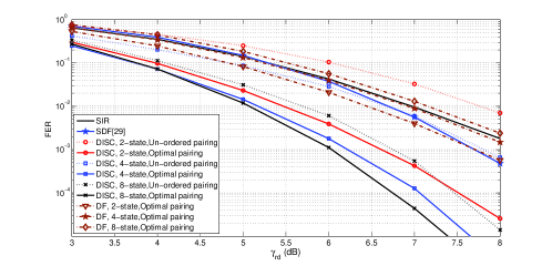
Figure 5: FER for 2 relays in AWGN Channels, ${\bar{\gamma}_{sr}}={\bar{\gamma}_{s{r_{1}}}}={\bar{\gamma}_{s{r_{2}}}}-3dB$, ${\bar{\gamma}_{sr}}={\bar{\gamma}_{rd}}$.

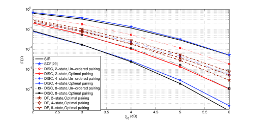
Figure 6: FER for 2 relays in AWGN channels, ${\bar{\gamma}_{sr}}={\bar{\gamma}_{s{r_{1}}}}={\bar{\gamma}_{s{r_{2}}}}-3dB$, ${\bar{\gamma}_{sr}}={\bar{\gamma}_{rd}}+3dB$.

IV Simulation Results and Discussions

In this section, we present the simulation results. All simulations are performed for the BPSK modulation and a frame size of 130 symbols over AWGN and quasi-static fading channels. We assume that all relays use the code with the same number of states. Thus if there are K relays, the convolutional code of rate 1/K with K constituent codes can be used in K relays, and each relay uses one constituent code. For example, for the relay network with 2, 3 and 4 relays, the convolutional codes listed in Table 1 can be used as constituent codes at the relays. All schemes are compared under the same power constraint.

Figs. 5-6 compare the frame error rate (FER) performance of the proposed DISC with optimum and un-ordered code pairing, soft information relaying (SIR) [6], soft decode and forward (SDF) [29] as well as the conventional detect and forward (DF) with relay re-encoding (DF) for various numbers of states over AWGN channels for ${\bar{\gamma}_{sr}}={\bar{\gamma}_{rd}}$, ${\bar{\gamma}_{sr}}={\bar{\gamma}_{rd}}$+3dB, respectively. We set ${\bar{\gamma}_{s{r_{1}}}}={\bar{\gamma}_{sr}}$ and ${\bar{\gamma}_{s{r_{2}}}}={\bar{\gamma}_{sr}}+3dB$. Here the optimal and un-ordered assignment is the same as the assignment given in Example 2. We assume in the SIR scheme that the overall destination noise follows the Gaussian distribution and the maximum ratio combining (MRC) is used to combine received signals from all relays.

We can first note from these figures that the performance of the DF with relay encoding gets worse as the number of relay encoder states increases. Such performance degradation is due to the error propagations in the DF scheme. In the DF scheme, when detection errors occur at the relays, the re-encoding process causes errors to propagate into subsequent symbols. The longer the encoder memory, the larger the number of subsequent symbols affected by the detection errors. Therefore, the error rate of the DF will increase with the number of states. For example, Fig. 5 shows that the FER performance of the DF for the 4-state and 8-state codes is worse by 0.5dB and 0.7dB, respectively, than for the 2-state code at the FER of $10^{-3}$. However, the SISO encoder in the proposed DISC scheme can effectively mitigate the error propagation in the relay encoding process and at the same time provide a significant distributed coding gain. As a result, the DISC provides significant coding gains compared to the SIR without relay encoding and SDF scheme [29]. The gain increases as the number of states increases at high SNR. For example, as shown in Fig. 6, the DISCs with 2, 4 and 8-state are superior to the SIR and SDF scheme by about 1.7dB, 2.4dB and 2.5dB respectively. This result is consistent with the analysis in Section 3, showing that the DISC performance improves as the number of states at the relay encoder increases. Furthermore, we can also see from the figures that the DISC with optimal code pairing also brings significant gains compared to the DISC with the un-ordered pairing. For example, as shown in Fig. 5, the 4-state code with the optimal code pairing is superior to that with the un-ordered pairing by 2dB at the FER of $10^{-3}$. This validates the effectiveness of the proposed design criteria. Since the performance of the DISC with the un-ordered code pairing is exactly the same as the SISO encoding scheme in [8], the proposed scheme significantly outperforms the SISO encoding scheme in [8] and the gain comes from the optimal code paring.

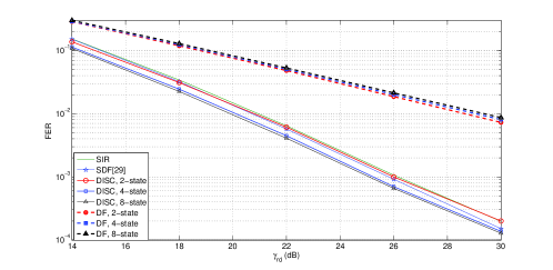
Figure 7: FER for 2 relays in fading channels, ${\bar{\gamma}_{sr}}={\bar{\gamma}_{s{r_{1}}}}={\bar{\gamma}_{s{r_{2}}}}$, ${\bar{\gamma}_{sr}}={\bar{\gamma}_{rd}}$.

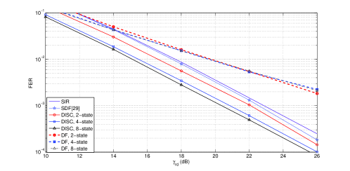
Figure 8: FER for 2 relays in fading channels, ${\bar{\gamma}_{sr}}={\bar{\gamma}_{s{r_{1}}}}={\bar{\gamma}_{s{r_{2}}}},{\bar{\gamma}_{sr}}={\bar{\gamma}_{rd}}+10dB$.

Figs. 7-8 compare the performance over fading channels for a network with 2 relays for ${\bar{\gamma}_{sr}}={\bar{\gamma}_{rd}}$, ${\bar{\gamma}_{sr}}={\bar{\gamma}_{rd}}$ +10dB, respectively. We set ${\bar{\gamma}_{s{r_{1}}}}={\bar{\gamma}_{s{r_{2}}}}={\bar{\gamma}_{sr}}$. It can also be observed from the figures that the DISC and SIR can achieve the full diversity order of 2, but the conventional DF can only achieve the diversity order of 1 due to error propagation. These two figures also compare the performance of DISC with SIR without relay re-encoding. It can be seen that the DISC substantially outperforms SIR. For example, the DISC with 2, 4 and 8 states can bring about 0.1dB, 0.8dB and 1dB gains, respectively, relative to the SIR scheme, for ${\bar{\gamma}_{sr}}={\bar{\gamma}_{rd}}$ and the gains are increased to 1dB, 2dB and 2.5dB, respectively, for ${\bar{\gamma}_{sr}}={\bar{\gamma}_{rd}}$+10dB. That is, the coding gain brought by the DISC increases when the source-relay link quality is improved. We can also observe that the coding gain increases as the number of relay encoder states increases.

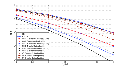
Figure 9: FER for 3 relays in AWGN Channels, ${\bar{\gamma}_{sr}}={\bar{\gamma}_{s{r_{1}}}}={\bar{\gamma}_{s{r_{2}}}}-2dB={\bar{\gamma}_{s{r_{3}}}}-4dB$, ${\bar{\gamma}_{sr}}={\bar{\gamma}_{rd}}$.

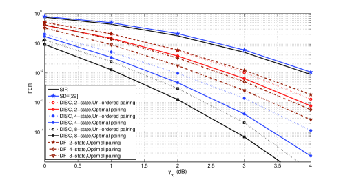
Figure 10: FER for 3 relays in AWGN Channels, ${\bar{\gamma}_{sr}}={\bar{\gamma}_{sr,1}}={\bar{\gamma}_{s{r_{2}}}}-2dB={\bar{\gamma}_{s{r_{3}}}}-4dB$, ${\bar{\gamma}_{sr}}={\bar{\gamma}_{rd}}+3dB$.

Figs. 9-12 show the results for three relays over AWGN and fading channels, respectively. From these figures we can observe similar trends as for the case with two relays. That is, the DISC can bring significant gains over the SIR, SDF and DF with re-encoding on both AWGN and fading channels and the gains increase as the number of state increases. For the fading channels, both DISC and SIR schemes can achieve the full diversity order of 3 while the DF can only achieve the diversity order of 1. Also pairing can bring system considerable gains over AWGN channels. Furthermore, the coding gain of DISC over SIR slightly increases as the number of relay increases from 2 to 3.

From the above results, we can see that the relay encoding in the conventional DF schemes cause serious error propagation and thus does not provide any coding advantages. By contrary, the proposed DISC can effectively mitigate the error propagation in the relay encoding and provide significant distributed coding gains, thus substantially outperforming the soft information relaying (SIR) and conventional DF schemes.

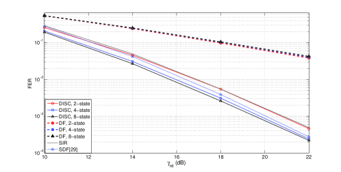
Figure 11: FER for 3 relays in fading channels, ${\bar{\gamma}_{sr}}={\bar{\gamma}_{sr,1}}={\bar{\gamma}_{s{r_{2}}}}={\bar{\gamma}_{s{r_{3}}}},{\bar{\gamma}_{sr}}={\bar{\gamma}_{rd}}$.

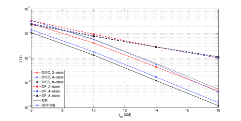
Figure 12: FER for 3 relays in fading channels, ${\bar{\gamma}_{sr}}={\bar{\gamma}_{sr,1}}={\bar{\gamma}_{s{r_{2}}}}={\bar{\gamma}_{s{r_{3}}}},{\bar{\gamma}_{sr}}={\bar{\gamma}_{rd}}+10dB$.

V Conclusions

In this paper we proposed a new distributed soft coding (DISC) scheme based on a soft input soft output encoder at the relay and the optimal design criteria were proposed. The proposed scheme performs encoding of the noisy source symbol estimates in error-prone relay channels. It can effectively circumvent error propagation in the relay encoding process and at the same time provide significant distributed coding gains. It provides great performance improvement compared to the soft information relaying (SIR) and conventional DF schemes. At high SNR the gain further increases as the number of state increases.

In the analysis and simulations of DISC in this paper we approximated the distribution of the overall destination noise as the Gaussian distribution. As shown in [7, 34], the actual distribution does not follow the exact Gaussian distribution. Further improvement can be expected when the accurate distribution of the overall destination noise is derived, but unfortunately it has been a quite challenging topic so far.

VI Acknowledgement

We would like to all the reviewers for their valuable comments and suggestions for improving the quality of the paper. We also would like to thank Dr. Ingmar Land for the thoughtful discussions about the error modeling in DF scheme.

VII Appendix

VII-A Proof of Theorem 1

To prove this theorem, let us first prove the following Lemma.

Lemma 1: Let $c(i)$ be the $i$-th output symbol of a binary encoder generated by $\mathbf{G}$ for source binary sequence $\bf{b}=\left({b(1),\cdots,b(N)}\right)$. It is given by

$$c(i)={{\bf{G}}_{i}}{{\bf{b}}^{T}}=\sum\limits_{n=1}^{N}{G_{in}b(n)},$$ (36)

where the summation is over GF(2). Let ${l_{b}}(n)=\ln\left({\Pr(b(n)=0)/\Pr(b(n)=1}\right)$ represent the log likelihood ratio (LLR) of $b(n)$. Then the LLR of $c(i)$, denoted by ${l_{c}}\left(i\right)$, can be calculated as follows

$${l_{c}}\left(i\right)=\ln\frac{{\Pr(c(i)=0)}}{{\Pr(c(i)=1)}}=\ln\frac{{1+\prod\nolimits_{n\in{U_{i}}}{\tanh\left({{l_{b}}(n)/2}\right)}}}{{1-\prod\nolimits_{n\in{U_{i}}}{\tanh\left({{l_{b}}(n)/2}\right)}}},$$ (37)

where $\tanh(x)=\frac{{{e^{2x}}-1}}{{{e^{2x}}+1}}$.

The Lemma 1 can be directly proved by using the L-algebra [19]

$$l\left({b({n_{1}})\oplus b({n_{2}})\cdots\oplus b({n_{k}})}\right)~{}~{}~{}~{}~{}~{}~{}$$

$$=\ln L\left({b({n_{1}})\oplus b({n_{2}})\cdots\oplus b({n_{k}})}\right)$$

$$=\ln\frac{{1+\prod\nolimits_{q=1}^{k}{\tanh({l_{b}}({n_{q}})/2)}}}{{1-\prod\nolimits_{q=1}^{k}{\tanh({l_{b}}({n_{q}})/2)}}},~{}~{}~{}~{}$$ (38)

where $L(x)$ and $l(x)$ denote the likelihood ratio and LLR of $x$, respectively.

From Lemma 1, we can easily prove the Theorem 1. Let ${\tilde{x}_{b}}(k)$ and ${l_{b}}\left(k\right)$ represent the SBE and LLR of source bit $b(k)$. Then they have the following relationship,

$${l_{b}}\left(k\right)=\ln\frac{{1+{{\tilde{x}}_{b}}(k)}}{{1-{{\tilde{x}}_{b}}(k)}},$$ (39)

$${\tilde{x}_{b}}(k)=\tanh\left({{l_{b}}(k)/2}\right)=\frac{{\exp\left({{l_{b}}(k)}\right)-1}}{{\exp\left({{l_{b}}(k)}\right)+1}}.$$ (40)

By substituting Eq. (40) into (37), we have

$${l_{c}}\left(i\right)=\ln\frac{{1+\prod\nolimits_{j\in{U_{i}}}{{{\tilde{x}}_{b}}(j)}}}{{1-\prod\nolimits_{j\in{U_{i}}}{{{\tilde{x}}_{b}}(j)}}}.$$ (41)

Then by using the relationship of the SBE and LLR in Eq. (40), the SBE of $c(k)$, denoted by ${\tilde{x}_{c}}(k)$, can be calculated as

$${\tilde{x}_{c}}(k)=\prod\nolimits_{j\in{U_{k}}}{{{\tilde{x}}_{b}}(j)}=\exp\left({{{\bf{G}}_{k}}{{\left({{\bf{ln}}{{{\bf{\tilde{x}}}}_{b}}}\right)}^{T}}}\right).$$ (42)

This proves Theorem 1.

VII-B Proof of Theorem 3

To prove the theorem, we need to use the following Lemma.

Lemma 2: Given the positive real numbers ${v_{1}}>{v_{2}}>0$ and ${\theta_{1}}>{\theta_{2}}>0$, the following relationship always holds,

$$\frac{1}{{{v_{1}}+{\theta_{1}}}}+\frac{1}{{{v_{2}}+{\theta_{2}}}}>\frac{1}{{{v_{1}}+{\theta_{2}}}}+\frac{1}{{{v_{2}}+{\theta_{1}}}}.$$ (43)

The proof of the above result is straightforward and we omit it here. Now let us use the Lemma to prove Theorem 3.

Since ${\gamma_{r_{k}{d}}}={\gamma_{rd}}$ for all $k=1,\ldots,K$, we can rewrite ${\rho_{k}}\left({d_{k},{\gamma_{rd}},{\gamma_{s{r_{k}},in}}}\right)$ as follows

$${\rho_{k}}\left({d_{k},{\gamma_{rd}},{\gamma_{s{r_{k}},in}}}\right)=\frac{{{\gamma_{rd}}{\gamma_{s{r_{k}},in}}}}{{{\gamma_{s{r_{k}},in}}d_{k}^{-1}+{\gamma_{rd}}}}$$

$$=\frac{1}{{{{\left({d_{k}{\gamma_{rd}}}\right)}^{-1}}+{{\left({{\gamma_{sr_{k},in}}}\right)}^{-1}}}}=\frac{1}{{\left({{v_{k}}+{\theta_{k}}}\right)}},$$ (44)

where ${v_{k}}={\left({d_{k}{\gamma_{rd}}}\right)^{-1}}$ and ${\theta_{k}}={\left({{\gamma_{s{r_{k}},in}}}\right)^{-1}}$.

Let ${v_{(1)}}$, ${v_{(2)}}$, …,${v_{(K)}}$ and ${\theta_{(1)}}$, ${\theta_{(2)}}$, …,${\theta_{(K)}}$ represent the re-ordered values of ${v_{1}}$, ${v_{2}}$, …,${v_{K}}$ and ${\theta_{1}}$, ${\theta_{2}}$, …,${\theta_{K}}$. Then from Eqs. (25) and (26), we have

$${v_{(1)}}\leq{v_{(2)}}\cdots\leq{v_{(K)}}~{}and~{}{\theta_{(1)}}\leq{\theta_{(2)}}\cdots\leq{\theta_{(K)}}.$$ (45)

Now let us determine how to distribute $\{{v_{(1)}},\cdots,{v_{(K)}}\}$ and $\{{\theta_{(1)}},\cdots,{\theta_{(K)}}\}$ to form $K$ pairs $\left({{v_{k}},{\theta_{k}}}\right)$, $k=1,\ldots,K$, where any ${v_{(i)}}$ or ${\theta_{(j)}}$ can only be assigned to one and only one pair, so as to maximize $\sum\limits_{k=1}^{K}{{\rho_{k}}\left({d_{k},{\gamma_{rd}},{\gamma_{sr_{k},in}}}\right)}$. As can be seen from Eq. (44), this is equivalent to maximizing

$${\Sigma_{K}}=\sum\limits_{k=1}^{K}{\frac{1}{{{v_{k}}+{\theta_{k}}}}}=\sum\limits_{k=1}^{K}{f\left({{v_{k}},{\theta_{k}}}\right)},$$ (46)

where $f\left({{v_{k}},{\theta_{k}}}\right)={({v_{k}}+{\theta_{k}})^{-1}}$.

We assume that the optimal $K$ pairs of for $k=1,\ldots,K$, are $\left({{v_{(1)}},{\theta_{{j_{1}}}}}\right)$, $\left({{v_{(2)}},{\theta_{{j_{2}}}}}\right)$,$\ldots$, $\left({{v_{(K)}},{\theta_{{j_{K}}}}}\right)$. Now we prove this theorem by contradiction. Assume that ${\theta_{{j_{1}}}},{\theta_{{j_{2}}}},\ldots,{\theta_{{j_{K}}}}$ do not exactly follow the relationship of ${\theta_{{j_{1}}}}\leq{\theta_{{j_{2}}}}\cdots\leq{\theta_{{j_{K}}}}$. Then there must exist at least two integers $p,q$, such that ${\theta_{{j_{p}}}}>{\theta_{{j_{q}}}}$ for $p<q$. Since ${v_{(q)}}\geq{v_{(p)}}$ and ${\theta_{{j_{p}}}}>{\theta_{{j_{q}}}}$, then by using the Lemma 1, we have

$$f\left({{v_{(q)}},{q_{{j_{p}}}}}\right)+f\left({{v_{(p)}},{\theta_{{j_{q}}}}}\right)>f\left({{v_{(q)}},{\theta_{{j_{q}}}}}\right)+f\left({{v_{(p)}},{\theta_{{j_{p}}}}}\right).$$ (47)

This means that when we switch ${\theta_{{j_{q}}}}$ and ${\theta_{{j_{p}}}}$ in the two pairs $\left({{v_{(p)}},{\theta_{{j_{p}}}}}\right)$ and $\left({{v_{(q)}},{\theta_{{j_{q}}}}}\right)$, leading to a new two pairs $\left({{v_{(p)}},{\theta_{{j_{q}}}}}\right)$ and $\left({{v_{(q)}},{\theta_{{j_{p}}}}}\right)$, while keeping other pairs unchanged, the resulted ${\Sigma_{K}}$ will be larger. This contradicts that $\left({{{\bf{v}}_{(1)}},{\theta_{{j_{1}}}}}\right),\cdots,\left({{v_{(K)}},{\theta_{{j_{K}}}}}\right)$ are the optimal pairs achieving the maximum ${\Sigma_{K}}$. Therefore, the optimal pairs are $\left({{v_{(1)}},{\theta_{(1)}}}\right),\left({{v_{(2)}},{\theta_{(2)}}}\right),\cdots,\left({{v_{(K)}},{\theta_{(K)}}}\right)$. This proves Theorem 3.

References

- [1] J. N. Laneman, D. N. C. Tse, and G. W. Wornell, ”Cooperative diversity in wireless networks: efficient protocols and outage behavior,” IEEE Trans. IT, vol. 50, pp. 3062-2080, Dec. 2004.
- [2] G. Kramer, M. Gastpar, and P. Gupta, ”Cooperative strategies and capacity theorems for relay networks,” IEEE Trans. IT, vol. 51, pp. 3037-3063, Sept. 2005.
- [3] T. M. Cover and A. A. El Gamal, ”Capacity theorems for the relay channel,” IEEE Trans. IT, vol. 25, pp. 572-584, Sept. 1979.
- [4] H. H. Sneessens and L. Vandendorpe, ”Soft decode and forward improves cooperative communications,” Proc of 6th IEE International Conference in 3G and Beyond, pp. 1-4, Nov. 7-9, 2005, London, November 2005.
- [5] X. Bao and J. Li, ”Efficient message relaying for wireless user cooperation: decode-amplify-forward (DF) and hybrid DF and coded-cooperation,” IEEE Trans Wireless Commun., vol. 6, pp. 3975-3984, Nov. 2007.
- [6] K. S. Gomadam and S. A. Jafar, ”Optimal relay functionality for SNR maximization in memoryless relay networks,” IEEE JSAC, vol. 25, pp. 390-401, Feb. 2007.
- [7] P. Weitkemper, D. Wübben, V. Kühn, and K.-D. Kammeyer, ”Soft information relaying for wireless networks with error-prone source-relay link,” Proc. Int. ITG Conf. on Source and Channel Coding, Ulm, Germany, Jan. 2008.
- [8] Y. Li, B. Vucetic, T. F. Wong, and M. Dohler, ”Distributed turbo coding with soft information relaying in multihop relay networks,” IEEE JSAC, vol. 24, pp. 2040-2050, Nov. 2006.
- [9] Y. Li and B. Vucetic, ”On the performance of a simple adaptive relaying protocol for wireless relay networks,” Proc of VTC Spring 2008, Singapore, May 2008.
- [10] L. Lampe, R. Schober, and S. Yiu, ”Distributed space-time coding for multihop transmission in power line communication networks,” IEEE JSAC, vol. 24, no. 7, pp. 1389 - 1400, July 2006.
- [11] Y. Jing and B. Hassibi, ”Distributed space-time coding in wireless relay networks,” IEEE Trans. on Wireless Communications, vol. 5, pp. 3524-3536, Dec. 2006.
- [12] Y. Li and X. G. Xia, ”A family of distributed space-time trellis codes with asynchronous cooperative diversity,” Proc of IPSN 2005, Los Angeles, California, pp. 340 - 347, April 2005.
- [13] J. Yuan, Z. Chen Y. Li, and L. Chu, ”Distributed space-time trellis codes for a cooperative system,” IEEE Trans. on Wireless Communications, vol. 8, pp. 4897-4905, Aug 2009.
- [14] A. Chakrabarti, A. Baynast, A. Sabharwal, and B. Aazhang, ”Low density parity check codes for the relay channel,” IEEE JSAC, vol. 25, no.2, pp.280 - 291, Feb 2007.
- [15] H. Jun and T. Duman, ”Low density parity check codes over wireless relay channels,” IEEE Trans. Wireless Commun., vol. 6, no.9, pp. 3384 - 3394, Sept. 2007.
- [16] B. Zhao and M. C. Valenti, ”Distributed turbo coded diversity for relay channel,” Electron. Lett., vol. 39, no. 10, pp. 786-787, May 2003.
- [17] M. Janani, A. Hedayat, T. Hunter, and A. Nosratinia, ”Coded cooperation in wireless communications: space-time transmission and iterative decoding,” IEEE Trans. Signal Processing, vol. 52, pp.362 - 371, Feb. 2004.
- [18] P. Razaghi and W. Yu, ”Bilayer low-density parity-check codes for decode-and-forward in relay channels,” IEEE Trans. IT, vol. 53, no. 10, pp. 3723-3739, Oct. 2007.
- [19] J. Hagenauer, E. Offer, and L. Papke, ”Iterative decoding of binary block and convolutional codes,” IEEE Trans. IT, vol. 42, no. 2, pp. 429-445, March 1996.
- [20] K. J. Larsen, ”Short convolutional codes with maximal free distance for rate 1/2, 1/3, and 1/4,” IEEE Trans. IT, vol. 19, pp. 371-372, May 1973.
- [21] M. Dohler and Y. Li, Cooperative communications: hardware, channel and PHY, John Wiley 2010.
- [22] S. Lin and D. J. Costello, Error control coding, NJ: prentice hall, second ed., 2004.
- [23] A. Winkelbauer and G. Matz ”On efficient soft-input soft-output encoding of convolutional codes,” in Proc. ICASSP 2011, pp. 3132 - 3135, Prague, May, 2011.
- [24] M. Molu and N. Görtz, ”A study on relaying soft information with error prone relays,” in Proc. Allerton Conference on Communication, September, 2011.
- [25] T. Volkhausen, Dereje H. Woldegebreal, and H. Karl, ”Improving network coded cooperation by soft information,” In Proc. IEEE WiNC 2009, Jun. 2009.
- [26] Y. Peng, M. Wu, H. Zhao, and W. Wang, ”Cooperative network coding with soft information relaying in two-way relay channels,” Journal of communications, vol. 4, no. 11, pp.849-855, Dec. 2009.
- [27] W. Pu, C. Luo, S. Li, and C. W. Chen, ”Continuous network coding in wireless relay networks,” IEEE INFOCOM 2008, pp. 2198-2206.
- [28] F. Hu and J. Lilleberg, ”Novel soft symbol estimate and forward scheme in cooperative relaying networks,” in Proc. of PIMRC 2009.
- [29] K. Lee and L. Hanzo ”MIMO-assisted hard versus soft decoding-and-forwarding for network coding aided relaying systems,” IEEE Trans Wireless Commun., vol. 8, no. 1, Jan. 2009, pp. 376-385.
- [30] T. Wang, A. Cano, G. B. Giannakis, and N. Laneman, ”High-performance cooperative demodulation with decode-and-forward relays, IEEE Trans. Commun., vol. 55, no. 7, pp. 1427 1438, Jul. 2007.
- [31] P. Weitkemper, D. Wübben, and K.-D. Kammeyer, ”Minimum MSE relaying in coded networks,” in International ITG Workshop on Smart Antennas (WSA 08), Darmstadt, Germany, Feb 2008.
- [32] L.Bahl, J.Cocke, F.Jelinek, and J.Raviv, ”Optimal decoding of linear codes for minimizing symbol error rate,” IEEE Trans IT, vol. IT-20(2), pp.284-287, March 1974.
- [33] M. A. Karim, J. Yuan, Z. Chen, and J. Li ”Soft information relaying in fading channels,” IEEE Commun. Lett., vol. 1, no. 3, June 2012, pp. 233-236.
- [34] R. Thobaben and E. G. Larsson. ”Sensor-network-aided cognitive radio: On the optimal receiver for estimate-and-forward protocols applied to the relay channel,” Proc. of ACSSC , pp. 777-781, Nov. 2007.
- [35] E. Obiedat and L. Cao, ”Soft information relaying for distributed turbo product codes (SIR-DTPC), IEEE Signal Processing Lett., vol. Apr, 2010.
- [36] M. H. Azmi, J. Li, J. Yuan, and R. Malaney, ”LDPC codes for soft decode-and-forward in half-duplex relay channels,” to appear in IEEE JSAC.
- [37] I. Land, A. Graell i Amat, and L. K. Rasmussen, ”Bounding of MAP decode and forward relaying,” ISIT 2010, pp. 938-942, June 2010.
- [38] Z. Si, R. Thobaben, and M. Skoglund, ”On distributed serially concatenated codes,” in Proc. of Workshop on IEEE Signal Processing Advances in Wireless Communications, Jun. 2009, pp. 653 - 657.
- [39] M. Shirvanimoghaddam, Y. Li, and B. Vucetic, ”Distributed raptor coding for erasure channels: partially and fully coded cooperation,” to appear in IEEE Trans. Commun., accepted in July 2013.
- [40] M. Shirvanimoghaddam, Y. Li and B. Vucetic, ”User cooperation via rateless coding,” Globecom, Anaheim, CA, USA, Dec. 2012.
- [41] M. Shirvanimoghaddam, Y. Li and B. Vucetic, ”Distributed rateless coding with cooperative sources,” ISIT, Boston June 2012.
- [42] Y. Li, B. Vucetic, Z. Chen and J. Yuan, ”Distributed turbo coding with selective relaying,” PIMRC, Tokyo Japan, Sept 2009.
- [43] Y. Li, B. Vucetic, Z. Chen and J. Yuan, ”An improved relay selection scheme with hybrid relaying protocols,” GLOBECOM, Nov. 2007, pp. 3704 - 3708.
- [44] Y. Li, B. Vucetic and J. Yuan, ”Distributed turbo coding with hybrid relaying protocols,” IEEE PIMRC’08, France, Sept 2008.
- [45] T. Liu, L. Song, Y. Li, Q. Huo and B. Jiao, ”Performance analysis of hybrid relay selection in cooperative wireless systems,” IEEE Trans. Commun., vol. 60, no. 3, March 2012, pp. 779-788.
- [46] S. X. Ng, Y. Li and L. Hanzo, ”Distributed turbo trellis coded modulation for cooperative communications,” Proc of ICC 2009.
- [47] Y. Li, ”Distributed coding for cooperative wireless networks: an overview and recent advances,” IEEE Communications Magazine, pp. 71-77, no. 8, August 2009.
- [48] D. Liang, S. X. Ng and L. Hanzo, ”Relay-Induced Error Propagation Reduction for Decode-and-Forward Cooperative Communications”, Proc. of IEEE Globecom, Dec. 2010.
- [49] L. Kong, S. X. Ng, R. G. Maunder and L. Hanzo, ”Maximum-Throughput Irregular Distributed Space-Time Code for Near-Capacity Cooperative Communications”, IEEE Trans. Veh. Tech., vol. 59, no. 3, pp. 1511-1517, March 2010.