The class of nonlinear stochastic models as a background for the bursty behavior in financial markets
Abstract
We investigate behavior of the continuous stochastic signals above some threshold, bursts, when the exponent of multiplicativity is higher than one. Earlier we have proposed a general nonlinear stochastic model applicable for the modeling of absolute return and trading activity in financial markets which can be transformed into Bessel process with known first hitting (first passage) time statistics. Using these results we derive PDF of burst duration for the proposed model. We confirm derived analytical expressions by numerical evaluation and discuss bursty behavior of return in financial markets in the framework of modeling by nonlinear SDE.
1 Introduction
Most econometric analysis of financial markets based on the various versions of stochastic differential equations (SDEs) have been limited to the case when the exponent of noise multiplicativity is lower than [1]. This is related to the general econometric assumptions for the asset price process and existence of unique Martingale measure [2]. Nevertheless, Chan et al. [3] have shown, comparing varying econometric models of short-interest rate, that the models allowing multiplicativity of capture the volatility changes of short-term interest rates better than those with .
We have introduced a class of non-linear stochastic differential equations (SDEs) providing time series with power-law statistics, and most notably reproducing spectral density, [4, 5, 6]. The general expression of the proposed class of Ito SDEs is
| (1) |
Here is the stochastic process exhibiting power-law statistics, is the power-law exponent of the multiplicative noise, is the exponent of power-law probability density function (PDF), and is a standard Wiener process (the Brownian motion). Note that SDE (1) was used in the modeling of trading activity and absolute return of financial markets [7] and is defined in the dimensionless scaled time, , we denote the scaling constant as and will use the relation to the real time of financial markets as . Empirical value appropriate for the markets absolute return model was defined in [8].
Directly from the SDE (1) follows that the stationary probability density function (PDF) of this stochastic process is power-law, , with the exponent [9]. While in Refs. [10] and later more precisely in [11] it was shown that SDE (1) provides time series with power-law spectral density
| (2) |
Note that exponent of spectral density, , is defined only for . In case of the SDE (1) becomes identical to the geometric Brownian motion and in case one gets noise. Do not be confused by cumulative inverse cubic law defined for return in [12], where .
Empirical data from the financial markets confirm the choice of equations (1) with [7] while modeling trading activity and absolute return. The case of represents the higher positive signal-to-noise feedback and leads to the faster than exponential changes, growth or descent, observed in the time series [13].
Our modeling of financial market variables using the non-linear stochastic differential equations is based on the empirical analysis and the power-law statistics of proposed equations [7]. Providing microscopic, agent-based, reasoning for the proposed equations seems to be a formidable task for such complex system. Apparently, the development of macroscopic descriptions for the well established agent based models would be more consistent approach towards the understanding of the micro and macro correspondence. For such analysis one should select simple agent based models with established or expected macroscopic description. First of all we expect that herding, contagion and cascading behavior of agents should lead to the macroscopic description with the non-linear stochastic differential equations.
The convenience of this approach is already confirmed by some recent publications considering this problem [14, 15, 6]. Kirman’s ant colony model [16] is an agent-based model, which explains the importance of herding. As human crowd behavior ideologically is very similar, the ant colony model actually was built as a general framework for financial market modeling [17, 18, 16]. In [14, 15, 6] we follow the works by Alfarano et al. [17, 18] to introduce model modifications, which allow us to obtain agent-based models for the financial markets exhibiting a macroscopic description in terms of SDEs with .
In this contribution we demonstrate that the general class of SDEs (1) can be transformed to the Bessel process, which represents a special family of diffusion models applicable in econometric analysis [1]. This allows us to derive explicit form of burst statistics generated by the SDE (1). Exponent of multiplicativity is a key parameter of defined statistics. We also present analysis of empirical data providing an evidence that burst statistics of return in financial markets can be modeled by non-linear stochastic differential equations with multiplicativity as high as .
2 Statistics of stochastic bursty time series
Looking for the best form of SDE applicable to the modeling of complex systems one has to use the most distinct features of the observed behavior. Spikes, bubbles or bursts of the observed signals is one of the characteristic features of complex systems, as well as 1/f noise. Well defined statistics of bursty behavior can serve as an additional source of information about the system. It is natural to expect that parameter of multiplicativity in Eq. (1) is responsible for the bursty behavior of defined stochastic signal. Therefore described statistics of bursty behavior would help establish relation between model parameters and empirical data. Although we concentrate here more on the return not price dynamics, such characteristics of bursts as duration and peak value should be indispensable in risk valuation process.
We define a burst as a part of time series lying above certain threshold, . In Fig. 1 we have presented an example burst of the simple bursty time series, (hence the threshold is denoted as ). Evidently a burst itself can be characterized by its duration, , peak value, , and burst size, defined as the area above the threshold yet bellow time series (highlighted), . One can also introduce inter-burst, , and waiting, , times to be able to fully grasp the statistical features of bursty behavior. We will derive the explicit form PDF of burst duration , generated by Eq. (1), and will analyze numerically correspondence with empirical data of returns and relations to the other statistical characteristics of bursty behavior.
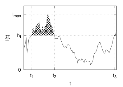
There is a well established hitting (passage) time framework, which is of high interest in both mathematical finance [1] and physics [9, 19]. This framework can be also applied in the description of burst duration PDF. Actually first hitting time of the stochastic process starting infinitesimally near above the hitting threshold is the same as burst duration. It is so as the first passage of threshold ends the burst by its definition.
2.1 Numerical and empirical definitions of bursty behaviour statistics
In this contribution we consider stochastic model driven by SDE (1) and empirical time series of absolute return. Let us present a brief discussion on how we deal with the numerical and empirical time series.
SDE (1) serves as a most simple definition of very wide class of stochastic processes with power law statistics for high values of the signal intensity, . Any real system with corresponding power law statistics of high values has to be restricted from the side of small values. One can consider reflecting boundary condition at the point as the most simple case. Nevertheless, the more general approach can be implemented by wide choice of compressed exponential restrictions, which can be introduced by additional term in SDE (1)
| (3) |
Here denotes the diffusion restriction point and defines how sharp restriction is. Steady state distribution of is as follows
| (4) |
As we analyze bursts, behavior in the region of high values of , it is reasonable to assume and . With such assumption we numerically solve (3) by evaluating the difference equations:
| (5) | |||
| (6) |
here is a normally distributed random variable with unit variance and zero mean, is a numerical precision parameter (it should be significantly smaller than 1). The above difference equations follow from the Euler-Maruyama method for the numerical solution of the stochastic differential equations [20] with variable time steps. Looking for the higher precision one may alternatively choose Milstein method [20].
We iterate through the (5) and (6) until we obtain time series with set amount of bursts. The suitable precision was achieved from time series with bursts. We choose threshold value to ensure sufficient number of burst and as well defined empirical exponent of return distribution [12], in our all numerical calculations.
Our empirical data set includes all trades made on NYSE, which were made from January, 2005 to March, 2007 and involved 24 different stocks, ABT, ADM, BMY, C, CVX, DOW, FNM, GE, GM, HD, IBM, JNJ, JPM, KO, LLY, MMM, MO, MOT, MRK, SLE, PFE, T, WMT, XOM. We have shown in [7] that the more sophisticated versions of (3) may be well used to model absolute return and trading activity of different stocks from NYSE and Vilnius Stock Exchange. In this approach the normalized absolute return time series of different stocks served as independent realizations of the stochastic process driven by the same nonlinear SDE with the same set of parameters. Such universal nature of stock market return behavior is hidden under secondary high frequency stochastic process with the -Gaussian PDF.
The double stochastic nature of the return makes analysis of the bursty behavior in empirical stock data as a more complex task. One minute return time series are very noisy, see [7] for more details. This noise of normalized time series can be diminished by using moving average filter. We have used one hour window moving average filter on the empirical data of one minute absolute returns. Time series of all stocks were used to define statistics of burst durations, peak values and sizes.
2.2 Obtaining probability density function of burst durations using the first hitting times of Bessel process
There are few simple and highly applicable models for which hitting times statistics are known. These models include, but are not limited to, Brownian motion, geometric Brownian motion and Bessel process [1]. The Bessel process,
| (7) |
is one of the most interesting as some prominent mathematical finance models can be transformed to a similar form. Bessel process is also interesting in Physics since it describes the evolution of the Euclidean norm, , of the -dimensional Brownian particle. The widely used parameter ,
| (8) |
is known as the index of the Bessel process related to the -dimensional Brownian diffusion. Note that for , or alternatively , tends to diverge towards infinity.
One can reduce (1) to Bessel process by using Lamperti transformation, . The exact form of transformation can be obtained by requiring that
| (9) |
Note that this requirement follows from the the Ito variable substitution formula [9]. Thus the Lamperti transformation has the following form
| (10) |
In such case the stochastic differential equation (1) can be transformed to the Bessel process,
| (11) |
with index . The dimension of the obtained Bessel process is given by .
Let us assume that a burst starts at time , thus exceeds the threshold, , by some small amount. The burst lasts until crosses back , from the above. Equivalently, in the terms of Bessel process the burst lasts until at a certain time, , the process crosses the boundary from the below, while the starting position, , in terms of Bessel process also lies below the threshold, . We see that the burst durations of the stochastic process driven by SDE (1) is related to the well known first passage times of the Bessel process.
By choosing arbitrarily close yet below , we can obtain an estimate for the burst duration, , in terms of first passage times of the Bessel process, :
| (12) |
where is an arbitrary small positive constant. As given in [21], the following holds for :
| (13) |
where is a probability density function of the first passage times at level of Bessel process with index starting from , is a Bessel function of the first kind of order and is a -th zero of .
We have to replace by density function regarding to avoid trivial convergence of to zero, when . This is achieved introducing PDF as a probability density function of burst duration
| (14) |
where the threshold is set at level and is related to the model parameters (see discussion on the transformation to Bessel process). To evaluate the limit we have to expand near :
| (15) |
By using this expansion we can rewrite (14) as:
| (16) |
here is a normalization constant. Since are almost equally spaced [22], we can replace the sum by integration
| (17) |
Note that derived PDF in the form of Eqs. (16) or (17) diverge, when approaches zero. Therefore normalization constants and can be defined if some minimum value of is supposed. Accuracy of numerical calculations or minimum intertrade time can be considered as possible choices. From the above follows that the distribution of burst durations of SDE (1) can be approximated by a power-law with exponential cut-off according to
| (18) | |||
| (19) |
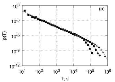
This result is in agreement with a general property of one dimensional diffusion processes presented in [19], namely that the asymptotic behavior of first hitting times is a power-law irrespectively of the nature of stochastic process or the actual form of Langevin and Fokker-Plank equations. The exponential cutoff for longer burst durations is caused by the direction preference, note the positive drift term in case of , or alternatively , of Bessel processes. Numerical solutions of the SDE (1) confirm the derived probability density function, (17), of the burst duration, , see Fig. 2 (a).
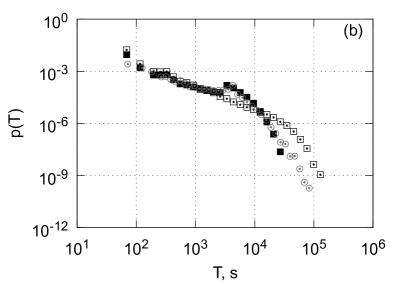
Empirical data, as shown in Fig. 2 (b), also has similar asymptotic behavior for short and long burst durations, though the fitting using (17) would be inconsistent for the intermediate burst durations, note the cusp. There are a numerous reasons for this. Firstly, we were unable to remove intra-day pattern from the empirical time series. But the main reason is that in order to reproduce the correct shape of the empirical probability density function for the intermediate values of one must use the double stochastic model, driven by a more sophisticated version of the SDE (1). In Fig. 2 (b) we demonstrate pretty good agreement of the probability density function of retrieved from the empirical NYSE time series and a more sophisticated double stochastic return model discussed in Appendix A.
2.3 Power law interdependencies between burst related variables
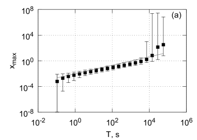
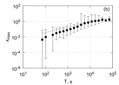
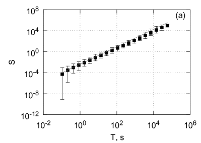
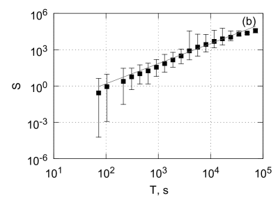
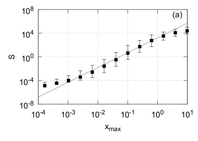
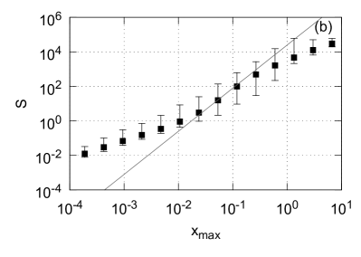
Another interesting feature of both numerical results and empirical data is that burst duration, peak value and burst size are correlated or even interdependent, . The scatter plots of these variables also reveal power-law asymptotic behavior - (see Fig. 3) and (see Fig. 4). Consequently, as follows from these relations (see Fig. 5). From SDE (1) numerically defined asymptotic relations are shown to hold for both empirical data and numerical results, though the theoretical power-law holds only in narrow region of empirical data. The interdependence between these variables suggest that the geometry of burst remains qualitatively the same in the fitted regions. Theoretical consideration of these relations in the region of PDF exponential cut-of will be continued.
3 Conclusions
Starting from the general expression of nonlinear SDE (1) and well-known PDF expression of first hitting time for Bessel process we have derived PDF of burst duration (16) and its approximation (17) for the nonlinear stochastic process driven by (1). The understanding of burst statistics is needed to enable efficient modeling of trading activity and return in financial markets based on the various versions of SDE (1) [7]. We do expect that proposed class of SDE is applicable in the modeling of other complex systems and defined statistics of bursts can be helpful in risk analyzes. We have also confirmed analytical results of burst statistics by numerical calculations of SDE (1), and compared it to the empirical data of return in financial markets. The obtained results encourage us to continue research of burst statistics in the financial markets seeking to develop more sophisticated versions of stochastic models. Most importantly we find that burst related statistical properties are related to the key parameter - exponent of stochastic multiplicativity characterizing the dynamics of risk in financial markets. Both numerical results and empirical data also reveal power-law asymptotic behavior of burst duration, peak value and burst size scatter plots. The exponents of observed power-law statistics probably have universal nature and will be considered in our future work.
Our analysis of empirical data suggests that long range fluctuations of absolute return in financial markets can be modeled by non-linear stochastic differential equations with up to .
Acknowledgments
We would like to thank Dr. Julius Ruseckas for valuable comments on the first draft of this work. The authors acknowledge the support by the EU COST Action MP0801 Physics of Competition and Conflicts stimulating our international cooperation.
Appendix A Double stochastic return model
The class of equations based on SDE (1) gives only a general idea how to model power-law statistics of trading activity and return in the financial markets. The problem is to determine the parameter set and , which would enable reproduction of the empirical values of and . The task becomes even more complicated if one considers the more sophisticated trends in the spectral density - power spectral densities have not a single, but two power-law regions with different values of . In the series of papers [23, 24, 8] we have shown that trading activity and return can be modeled by a more sophisticated stochastic differential equation than (1) now including the two powers of the noise multiplicativity. In the case of return instead of Eq. (1) one should use [8]
| (20) |
here divides the area of diffusion into the two different noise multiplicativity regions to ensure the spectral density of with two power law exponents, term gives the exponential diffusion restriction for large values of variable when .
The proposed form of the more complex SDE enables reproduction of the main statistical properties of the return observed in the financial markets. This provides an approach to the financial markets with behavior dependent on the level of activity and exhibiting two stages: calm and excited. One more peculiarity of the proposed model is that signal serves only as modulating one of secondary high frequency -Gaussian fluctuations. We formalized the empirical return in the model as instantaneous q-Gaussian fluctuations with a slowly diffusing parameter and constant
| (21) |
q-Gaussian distribution of can be expressed as follows:
| (22) |
The variable serves as a measure of instantaneous volatility of high frequency return fluctuations [8]. We proposed to model the measure of volatility by the scaled continuous stochastic variable , which can be interpreted as average return per unit time interval. Through the empirical analysis of high frequency empirical data from NYSE [8] we have introduced the following relation
| (23) |
where is an empirical parameter and the average return per unit time interval can be modeled by a nonlinear SDE (20), expressed in scaled dimensionless time .
References
- [1] M. Jeanblanc, M. Yor, and M. Chesney, Mathematical Methods for Financial Markets. Berlin: Springer, 2009.
- [2] D. Davydov and V. Linetsky, “Pricing and hedging path-dependent options under the cev process,” Management Science, vol. 47, pp. 949–965, 2001.
- [3] K. C. Chan, G. Andrew Karolyi, F. A. Longstaff, and A. B. Sanders, “An empirical comparison of alternative models of the short-term interest rate,” THE JOURNAL OF FINANCE, vol. XLVII, no. 3, pp. 1209–1227, 1992.
- [4] V. Gontis and B. Kaulakys, “Multiplicative point process as a model of trading activity,” Physica A, vol. 343, pp. 505–514, 2004.
- [5] B. Kaulakys, V. Gontis, and M. Alaburda, “Point process model of 1/f noise vs a sum of lorentzians,” Phys. Rev. E, vol. 71, no. 051105, pp. 1–11, 2005.
- [6] J. Ruseckas, B. Kaulakys, and V. Gontis, “Herding model and 1/f noise,” EPL, vol. 96, p. 60007, 2011.
- [7] V. Gontis, J. Ruseckas, and A. Kononovicius, A Non-Linear Double Stochastic Model of Return in Financial Markets, pp. 559–580. No. ISBN: 978-953-307-121-3, Sciyo, August 2010.
- [8] V. Gontis, J. Ruseckas, and A. Kononovičius, “A long-range memory stochastic model of the return in financial markets,” Physica A, vol. 389, pp. 100–106, 2010.
- [9] C. W. Gardiner, Handbook of stochastic methods. Berlin: Springer, 1997.
- [10] B. Kaulakys, J. Ruseckas, V. Gontis, and M. Alaburda, “Nonlinear stochastic models of 1/f noise and power-law distributions,” Physica A, vol. 365, pp. 217–221, 2006.
- [11] J. Ruseckas and B. Kaulakys, “1/f noise from nonlinear stochastic differential equations,” Physical Review E, vol. 81, p. 031105, 2010.
- [12] X. Gabaix, P. Gopikrishnan, V. Plerou, and H. E. Stanley, “Institutional investors and stock market volatility,” The Quarterly Journal of Economics, pp. 461–504, 2006.
- [13] S. Reimann, V. Gontis, and M. Alaburda, “Interplay between positive feedbacks in the generalized cev process,” Physica A: Statistical Mechanics and its Applications, vol. 390, no. 8, pp. 1393–1401, 2011.
- [14] V. Daniunas, V. Gontis, and A. Kononovicius, “Agent-based versus macroscopic modeling of competition and business processes in economics,” ICCGI 2011 : The Sixth International Multi-Conference on Computing in the Global Information Technology, pp. 84–88, 2011.
- [15] A. Kononovicius and V. Gontis, “Agent based reasoning for the non-linear stochastic models of long-range memory,” Physica A, vol. 391, no. 4, pp. 1309–1314, 2012.
- [16] A. P. Kirman, “Ants, rationality and recruitment,” Quarterly Journal of Economics, vol. 108, pp. 137–156, 1993.
- [17] S. Alfarano, T. Lux, and F. Wagner, “Estimation of agent-based models: The case of an asymmetric herding model,” Computational Economics, vol. 26, no. 1, pp. 19–49, 2005.
- [18] S. Alfarano, T. Lux, and F. Wagner, “Time variation of higher moments in a financial market with heterogeneous agents: An analytical approach,” Journal of Economic Dynamics and Control, vol. 32, pp. 101–136, 2008.
- [19] S. Redner, A guide to first-passage processes. Cambridge University Press, 2001.
- [20] P. E. Kloeden and E. Platen, Numerical Solution of Stochastic Differential Equations. Berlin: Springer, 1999.
- [21] A. N. Borodin and P. Salminen, Handbook of Brownian Motion. Basel, Switzerland: Birkhauser, 2 ed., 2002.
- [22] M. Abramowitz and I. A. Stegun, Handbook of Mathematical Functions with Formulas, Graphs, and Mathematical Tables. New York: Dover, 1972.
- [23] V. Gontis and B. Kaulakys, “Long-range memory model of trading activity and volatility,” J. Stat. Mech., vol. P10016, pp. 1–11, 2006.
- [24] V. Gontis, B. Kaulakys, and J. Ruseckas, “Trading activity as driven poisson process: comparison with empirical data,” Physica A, vol. 387, pp. 3891–3896, 2008.