Electron spin relaxation in rippled graphene with low mobilities

Abstract

We investigate spin relaxation in rippled graphene where curvature induces a Zeeman-like spin-orbit coupling with opposite effective magnetic fields along the graphene plane in ${\bf K}$ and ${\bf K}^{\prime}$ valleys. The joint effect of this Zeeman-like spin-orbit coupling and the intervalley electron-optical phonon scattering opens a spin relaxation channel, which manifests itself in low-mobility samples with the electron mean free path being smaller than the ripple size. Due to this spin relaxation channel, with the increase of temperature, the relaxation time for spins perpendicular to the effective magnetic field first decreases and then increases, with a minimum of several hundred picoseconds around room temperature. However, the spin relaxation along the effective magnetic field is determined by the curvature-induced Rashba-type spin-orbit coupling, leading to a temperature-insensitive spin relaxation time of the order of microseconds. Therefore, the in-plane spin relaxation in low-mobility rippled graphene is anisotropic. Nevertheless, in the presence of a small perpendicular magnetic field, as usually applied in the Hanle spin precession measurement, the anisotropy of spin relaxation is strongly suppressed.

I Introduction

In recent years, graphene has attracted much interest due to its potential for the all-carbon based electronics and spintronics.novoselov666 ; Tombros_07 ; Geim_07 ; castro ; peres2673 ; sarma407 ; ep-review ; wu-handbook ; FWang ; beenakker ; abergel ; shiraishia ; acik ; geim2011 A number of experiments on spin relaxation in graphene on SiO₂ substrate have been carried out, with spin relaxation times $\tau_{s}$ of the order of 10-100 ps reported.Tombros_07 ; han222109 ; Pi ; Jozsa_09 ; Tombros_08 ; Popinciuc ; han1012.3435 ; jo ; avsar Some works suggested the Elliott-Yafet (EY)ey mechanism to be dominant in spin relaxation,Jozsa_09 ; Popinciuc ; Tombros_08 ; han1012.3435 ; avsar ; jo while the surface chemical doping experiment supported the importance of the D’yakonov-Perel’ (DP)dp one.Pi These experiments have triggered intensive theoretical studies on spin relaxation in graphene.hernando146801 ; Castro_imp ; yzhou ; Fabian_SR ; dugaev085306 ; arxiv1107.3386 ; zhanggraphene ; jeong ; zhangdpey With inversion asymmetry, possibly caused by a perpendicular electric field or curvature, a Rashba-type spin-orbit coupling (SOC),Rashba which couples spin to pseudospin, arises in graphene.Kane_SOC ; Min ; Fabian_SOC ; Hernando_06 ; jeong ; abde It was found that with this SOC, the DP mechanism dominates the electron spin relaxation.hernando146801 Besides, it was revealed that for the EY mechanism, $\tau_{s}/\tau_{p}\sim n_{e}$, where $\tau_{p}$ is the momentum relaxation time and $n_{e}$ is the electron density.arxiv1107.3386 ; hernando146801 This makes the assessment, which attributes the observed linear relation between spin relaxation time $\tau_{s}$ and momentum relaxation time $\tau_{p}$ with the increase of electron density $n_{e}$ to the EY mechanism, in the experimental worksJozsa_09 ; Popinciuc ; Tombros_08 ; han1012.3435 ; avsar inappropriate.jo The magnitude of the Rashba-type SOC caused by a moderate perpendicular electric fieldFabian_SOC ; abde or curvatureHernando_06 ; jeong is of the order of $\mu$eV and the corresponding $\tau_{s}$ limited by the DP mechanism is as large as microseconds.yzhou The adatoms were suggested to enhance the local SOC to the order of 10 meV and hence provide a possible origin of the observed short spin relaxation time.Castro_imp ; abde ; varykhalov ; zhanggraphene ; zhangdpey ; Fabian_SR Recently, we set up a random Rashba model incorporating the effect of adatomszhangdpey and fitted the experimental data from different groups.Jozsa_09 ; Pi ; han1012.3435 ; jo We suggested that the DP mechanism dominates spin relaxation in graphene and can result in either linear or inversely linear relation between $\tau_{s}$ and $\tau_{p}$.zhangdpey

Very recently, Jeong et al. reported that curvature in graphene can lead to not only the Rashba-type SOC which is off-diagonal in the pseudospin space, but also an additional SOC diagonal in the pseudospin space.jeong This additional SOC serves as a Zeeman-like term with opposite magnetic fields in ${\bf K}$ and ${\bf K}^{\prime}$ valleys, similar to the case in carbon nanotube.izumida ; jeong075409 ; semenov Starting from the effective SOC, Jeong et al. studied spin relaxation in a chemically-clean corrugated graphene where the electron mean free path is much larger than the spatial range of the random spin-orbit fluctuation and the spatially averaged SOC is zero. Under such condition, the spin relaxation is solely limited by the spin-flip scattering due to the fluctuation of the SOC,glazov2157 ; sherman67 ; dugaev085306 as in the rippled graphene studied by Dugaev et al. where only the Rashba-type SOC was considered.dugaev085306 It is noted that in the two valleys, even though the effective magnetic fields from the Zeeman-like term are opposite, their contributions to the spin relaxation via the fluctuation-induced spin-flip scattering are independent and identical. Besides, it was found that the fluctuations of the Rashba-type SOC and the Zeeman-like term make comparable contribution to the spin relaxation, leading to a spin relaxation time at least of the order of 10 ns.jeong

Nevertheless, for low-mobility samples where the electron mean free path is smaller than the spatial range of the random spin-orbit fluctuation, the spin relaxation is determined by the local curvature-induced SOC.yzhourandom For each isolated valley, the Rashba-type SOC, together with the Zeeman-like term, still leads to a spin relaxation time of the order of microseconds in the DP mechanism. However, the two valleys are not independent any more due to the intervalley scattering. The opposite effective magnetic fields in two valleys, together with the intervalley scattering, give rise to another spin relaxation channel. This can be understood by a simple model. We label the spin vector in each valley as ${\bf S}_{\mu}$, where $\mu=\pm 1$ stands for the valley located at ${\bf K}$ or ${\bf K}^{\prime}$ point. The spin vector in each valley precesses around the effective magnetic field from the Zeeman-like term with a frequency ${\mbox{\boldmath$\omega$\unboldmath}}_{\mu}$, where ${\mbox{\boldmath$\omega$\unboldmath}}_{\mu}=-{\mbox{\boldmath$\omega$\unboldmath}}_{-\mu}$ and $|{\mbox{\boldmath$\omega$\unboldmath}}_{\mu}|=\omega$. The intervalley scattering is characterized by a scattering time $\tau_{v}$ between two valleys. The spin vectors ${\bf S}_{\mu}$, with the initial values ${\bf S}_{\mu}(0)={\bf S}_{-\mu}(0)={\bf S}_{0}$, satisfy the rate equations

$$\dot{\bf S}_{\mu}(t)+{\bf S}_{\mu}(t)\times{\mbox{\boldmath$\omega$\unboldmath}}_{\mu}+[{\bf S}_{\mu}(t)-{\bf S}_{-\mu}(t)]/\tau_{v}=0.$$ (1)

When ${\bf S}_{0}$ lies in the plane perpendicular to the effective magnetic field, one has the solution

$$\sum_{\mu}{\bf S}_{\mu}(t)=2{\bf S}_{0}e^{-t/\tau_{s}}$$ (2)

with $\tau_{s}=2/(\omega^{2}\tau_{v})$ in the strong intervalley scattering limit $\omega\tau_{v}\ll 1$. So far this mechanism has not been revealed in the literature.

In this work, we study the spin relaxation in the low-mobility rippled graphene (the mobility is around $2\times 10^{3}$ cm²/V$\cdot$s)avsar and take into account the above spin relaxation channel. The electron mean free path $l$ is smaller than the ripple size $\xi$. In the low temperature regime where the intervalley electron-phonon scattering is negligible, the spin relaxation is dominated by the Rashba-type SOC and $\tau_{s}$ is as large as microseconds. However, with the increase of temperature, due to the above spin relaxation channel, the relaxation time for spins polarized perpendicular to the effective magnetic field first decreases and then increases, with a minimum of several hundred picoseconds around room temperature.

This paper is organized as follows. In Sec. II, we present the model and Hamiltonian. In Sec. III, we study the spin relaxation in rippled graphene based on the kinetic spin Bloch equations (KSBEs).wu-review ; wu2945 ; wu373 The effect of temperature, impurity density and electron density on spin relaxation is investigated. The anisotropy of spin relaxation, without and with a small perpendicular magnetic field, is also addressed. We summarize in Sec. IV.

II Model and hamiltonian

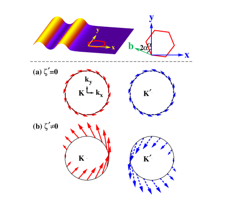
Figure 1: (Color online) Upper panel: schematic of the rippled graphene curved along the $x$-axis. The angle between the $y$-axis and one carbon-carbon bond in counterclockwise direction is $\alpha$ ($0\leq\alpha<2\pi/3$). Lower panel: schematic of the effective magnetic field from the SOC along one circle around ${\bf K}$ and ${\bf K}^{\prime}$ points. (a) The effective magnetic field induced by the Rashba-type SOC only ($\zeta^{\prime}=0$); (b) The effective magnetic field from both types of the SOC with $\alpha=0$.

The quasi-periodically rippled graphene can be synthesized by chemical vapor deposition on copper first and then transferred to the SiO₂ substrate perpendicular to the $z$-axis.avsar The surface morphology of the rippled graphene is illustrated in the upper panel of Fig. 1. The graphene is curved along the $x$-axis and we define the angle between the $y$-axis and one carbon-carbon bond in counterclockwise direction as $\alpha$ ($0\leq\alpha<2\pi/3$).jeong The size and height of the ripples are about 50 and 1 nm respectively.avsar The radius $R$ of curvature is 100-200 nm.avsar According to Ref. jeong, , the local effective SOC induced by the curvature reads

$$H_{\rm soc}=\zeta\kappa(\mu\tau_{x}\otimes\sigma_{y}-\tau_{y}\otimes\sigma_{x})+\mu\zeta^{\prime}\kappa I\otimes{\bf b}\cdot{\mbox{\boldmath$\sigma$\unboldmath}},$$ (3)

with ${\bf b}=(\cos(\pi/2+3\alpha),\sin(\pi/2+3\alpha),0)$ shown in the upper panel of Fig. 1. Here $\tau$ and $I$ are the Pauli matrices and unit matrix in the pseudospin space. $\sigma$ are the Pauli matrices in the spin space. The curvature $\kappa=R^{-1}$. The parameters $\zeta=0.15$ meV$\cdot$nm and $\zeta^{\prime}=0.21$ meV$\cdot$nm.jeong On the right-hand side of Eq. (3), the first term is the Rashba-type SOC reported previouslyHernando_06 and the second term is the additional Zeeman-like term diagonal in the pseudospin space.jeong

With the basis laid out in Refs. Fabian_SR, and yzhou, , the effective Hamiltonian of the electron band reads

$$H=\sum_{{\mu}{\bf k}ss^{\prime}}[\varepsilon_{\bf k}\delta_{ss^{\prime}}+(\bm{\Omega}_{\mu\bf k}+\frac{1}{2}g\mu_{B}{\bf B})\cdot{\mbox{\boldmath$\sigma$\unboldmath}}_{ss^{\prime}}]{c_{\mu{\bf k}s}}^{\dagger}c_{\mu{\bf k}s^{\prime}}+{H}_{\rm int}.$$ (4)

Here $c_{\mu{\bf k}s}$ (${c_{\mu{\bf k}s}}^{\dagger}$) is the annihilation (creation) operator of electrons in $\mu$ valley with momentum ${\bf k}$ (relative to the valley center) and spin $s$ ($s=\pm\frac{1}{2}$). $\varepsilon_{\bf k}=\hbar v_{f}k$ with $v_{f}=10^{6}$ m/s. $g\approx 2$ is the effective Landé $g$-factor,zhang136806 ; lukyanchuk176404 $\mu_{B}$ is the Bohr magneton and ${\bf B}$ is an external magnetic field perpendicular to the graphene plane (when it is applied, its magnitude is very small and the effect on orbital motionzhang136806 ; lukyanchuk176404 is negligible). The effective magnetic field from the SOC is given by

$$\bm{\Omega}_{\mu\bf k}=\zeta\kappa(-\sin\theta_{\bf k},\cos\theta_{\bf k},0)+\mu\zeta^{\prime}\kappa{\bf b},$$ (5)

where $\theta_{\bf k}$ is the polar angle of momentum ${\bf k}$. The second term on the right-hand side of the equation plays the role of the Zeeman-like term with the effective static magnetic field along ${\bf b}$ ($-{\bf b}$) in ${\bf K}$ (${\bf K}^{\prime}$) valley. The effective magnetic fields, without and with the second term, are schematically plotted in the lower panel of Fig. 1, where $\alpha$ is set as zero and hence ${\bf b}$ is along the $y$-aixs. The Hamiltonian $H_{\rm int}$ consists of both the intravalley and intervalley scatterings. The former include the electron-impurity,Adam_08 electron-remote-interfacial phonon,fratini electron-acoustic phonon,hwang1 electron–${\bf\Gamma}$-E_2g optical phononlazzeri as well as electron-electron Coulomb scatterings.yzhou The latter include the electron–${\bf K}$-A${}_{1}^{\prime}$ optical phononlazzeri and electron-electron Coulomb scatterings.yzhou

III Spin relaxation in rippled graphene

The KSBEswu2945 ; wu373 ; wu-review are utilized to study the spin relaxation in grahene,yzhou ; zhangdpey

$$\partial_{t}\rho_{\mu\bf k}(t)=\partial_{t}\rho_{\mu\bf k}(t)|_{\rm coh}+\partial_{t}\rho_{\mu\bf k}(t)|_{\rm scat},$$ (6)

where $\rho_{\mu\bf k}(t)$ represent the density matrices of electrons with relative momentum ${\bf k}$ in valley ${\mu}$ at time $t$. The coherent terms read $\partial_{t}\rho_{\mu\bf k}(t)|_{\rm coh}=-\frac{i}{\hbar}[(\bm{\Omega}_{\mu\bf k}+\frac{1}{2}g\mu_{B}{\bf B})\cdot{\mbox{\boldmath$\sigma$\unboldmath}},\rho_{\mu{\bf k}}(t)]$, where the Hartree-Fock term from the Coulomb interaction is neglected due to the small spin polarization.wu-review ; yzhou ; zhangdpey The concrete expressions of the scattering terms $\partial_{t}\rho_{\mu\bf k}(t)|_{\rm scat}$ are given in Ref. yzhou, . By solving the KSBEs, one obtains the spin relaxation time $\tau_{s}$ along direction ${\bf n}$ from the time evolution of spin polarization $P(t)=\frac{1}{n_{e}}\sum_{\mu{\bf k}}\mbox{Tr}[\rho_{\mu{\bf k}}(t){\mbox{\boldmath$\sigma$\unboldmath}}\cdot{\bf n}]$. In our calculation, unless otherwise specified, the initial spin polarization is $P(0)=10~{}\%$, the spin-polarization direction ${\bf n}$ is along the $z$-axis, the curvature $\kappa=0.01$ nm^-1, the electron density $n_{e}=7\times 10^{11}$ cm^-2, the impurity density $n_{i}=2\times 10^{12}$ cm^-2 and the external magnetic field ${\bf B}=0$. For spin relaxation along the $z$-axis, the direction of ${\bf b}$, determined by angle $\alpha$, is irrelevant.

III.1 Temperature dependence of spin relaxation

We first study the temperature dependence of the spin relaxation. In Fig. 2, the spin relaxation time $\tau_{s}$ is plotted against temperature $T$ at different curvatures $\kappa$. The electron mean free path $l$ is around 25 nm (the corresponding mobility is around $2.6\times 10^{3}$ cm²/V$\cdot$s) in the whole temperature regime investigated, as shown in Fig. 2 with the scale on the right-hand side of the frame. Therefore the electron mean free path is always smaller than the ripple size. It is indicated by this figure that when $T\leq 100$ K, $\tau_{s}$ is of the order of microseconds. However, when $T$ goes beyond 100 K, $\tau_{s}$ decreases rapidly to several hundred picoseconds at $T\sim 200$-$300$ K. Nevertheless, when $T$ further increases and exceeds the room temperature, $\tau_{s}$ begins to increase with $T$. It is also seen from the figure that $\tau_{s}$ reaches its minimum at a higher temperature with larger curvature $\kappa$. Moreover, when $T=50$ K and $T>250$ K, $\tau_{s}$ is proportional to $\kappa^{-2}$. However, in the intermediate temperature regime $100<T<250$ K, the spin relaxation times are nearly the same for different values of $\kappa$. This scenario is understood as follows.

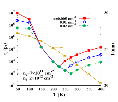
Figure 2: (Color online) Solid, dashed and dotted curves: temperature dependence of spin relaxation time with different values of $\kappa$. Chain curve with the scale on the right-hand side of the frame: temperature dependence of mean free path. $n_{e}=7\times 10^{11}$ cm^-2 and $n_{i}=2\times 10^{12}$ cm^-2.

We first focus on the case with $\kappa=0.01$ nm^-1. When $T\leq 100$ K, the intervalley scattering is negligibleyzhou and spins in two valleys relax independently. The spin relaxation is then determined by the Rashba-type SOC. The Zeeman-like term only serves as an in-plane effective magnetic field which mixes the in-plane and out-of-plane spin relaxations.dohrmann147405 It is known that with the Rashba-type SOC only and strong electron-impurity scattering, $\tau_{\perp}=\tau_{||}/2=\hbar^{2}/(4\zeta^{2}\kappa^{2}\tau_{p})$, where $\tau_{\perp}$ ($\tau_{||}$) is the out-of-plane (in-plane) spin relaxation time.Fabian_SR ; zhanggraphene Therefore in the presence of the effective magnetic field, the spin relaxation time along the $z$-axis is $\tau_{s}=2/(\tau_{\perp}^{-1}+\tau_{||}^{-1})=\hbar^{2}/(3\zeta^{2}\kappa^{2}\tau_{p})$. With $\tau_{p}=l/v_{f}$, one can estimate $\tau_{s}\approx 2.4~{}\mu$s at $T=50$ K, as shown in the figure. When $T$ increases, the intervalley electron–${\bf K}$-A${}_{1}^{\prime}$ optical phonon scattering becomes important and opens another spin relaxation channel together with the opposite effective magnetic fields in two valleys. According to the model presented in the introduction, in the weak intervalley scattering limit $\omega\tau_{v}\geq 1$ ($\omega=2\zeta^{\prime}\kappa/\hbar$ for the concrete situation here), one has the solution

$$\sum_{\mu}{\bf S}_{\mu}(t)=\frac{2{\bf S}_{0}e^{-t/\tau_{v}}}{\sqrt{1-(\omega\tau_{v})^{-2}}}\sin(\sqrt{\omega^{2}-\tau_{v}^{-2}}t+\phi)$$ (7)

with $\phi=\arctan\sqrt{\omega^{2}\tau_{v}^{2}-1}$ when ${\bf S}_{0}$ is perpendicular to the effective magnetic field. This indicates that the spin relaxation time is solely determined by the intervalley scattering time, i.e., $\tau_{s}=\tau_{v}$. Therefore, in the weak intervalley scattering limit, $\tau_{s}$ decreases with the enhancement of the intervalley scattering and hence the increase of $T$. However, in the strong intervalley scattering limit, $\tau_{s}=2/(\omega^{2}\tau_{v})$ as given by Eq. (2) in the introduction. In such case, $\tau_{s}$ increases with the increase of $T$. The crossover from the weak to strong intervalley scattering limit with the increase of $T$ is determined by $\tau_{v}^{-1}\approx\omega=2\zeta^{\prime}\kappa/\hbar$. At this crossover point, $\tau_{s}\approx\tau_{v}\approx\hbar/(2\zeta^{\prime}\kappa)$, which is estimated to be 170 ps, just as the value shown in the figure.

Based on the above analysis, it is understood that in the zero intervalley scattering limit $\tau_{s}=\hbar^{2}/(4\zeta^{2}\kappa^{2}\tau_{p})$ and in the strong intervalley scattering limit $\tau_{s}=\hbar^{2}/(2{\zeta^{\prime}}^{2}\kappa^{2}\tau_{v})$. In both limits $\tau_{s}$ is proportional to $\kappa^{-2}$. However, in the weak intervalley scattering limit with $\tau_{\perp}^{-1}\ll\tau_{v}^{-1}\leq\omega$, $\tau_{s}$ is determined by the intervalley scattering time $\tau_{v}$ and remains insensitive to $\kappa$. Besides, the crossover point in the nonmonotonic temperature dependence of spin relaxation time moves to a higher temperature with the increase of curvature $\kappa$ as determined by the relation $\tau_{v}^{-1}\approx 2\zeta^{\prime}\kappa/\hbar$. These properties manifest themselves in the curves with different values of $\kappa$ in Fig. 2.

III.2 Effect of intervalley scattering and SOC on spin relaxation

The intervalley scatterings include both the electron-electron Coulomb and electron-phonon scatterings.yzhou However, the essential role played in the spin relaxation channel revealed in this work is the intervalley electron-phonon scattering. That is because the intervalley Coulomb scattering which transfers electrons between the two valleys is negligible due to the large momentum transfer between them and hence the small scattering matrix element. Only the intervalley Coulomb scattering which does not lead to any electron transfer between the valleys is considered.yzhou

For comparison, we show the temperature dependence of spin relaxation time with different intervalley scatterings included in Fig. 3. It is seen that the intervalley Coulomb scattering is unimportant in the whole temperature regime under study while the intervalley electron-phonon scattering affects spin relaxation effectively. Particularly, when the intervalley electron-phonon scattering is excluded, $\tau_{s}$ becomes insensitive to $T$. That is because in the nearly isolated valleys, $\tau_{s}=\hbar^{2}/(3\zeta^{2}\kappa^{2}\tau_{p})$ with $\tau_{p}$ being dominated by the electron-impurity scattering.yzhou ; zhangdpey

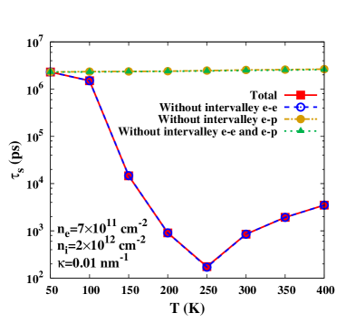
Figure 3: (Color online) Temperature dependence of spin relaxation time with the inclusion of different intervalley scatterings. Solid curve: with both the intervalley electron-electron (e-e) and electron-phonon (e-p) scatterings; Dashed curve: without the intervalley e-e scattering; Chain curve: without the intervalley e-p scattering; Dotted curve: without both the intervalley e-e and e-p scatterings. $n_{e}=7\times 10^{11}$ cm^-2, $n_{i}=2\times 10^{12}$ cm^-2 and $\kappa=0.01$ nm^-1.

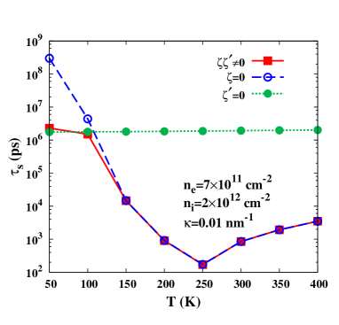
Figure 4: (Color online) Temperature dependence of spin relaxation time for the genuine case ($\zeta\zeta^{\prime}\neq 0$), the case without the Zeeman-like term ($\zeta^{\prime}=0$) and the case without the Rashba-type SOC ($\zeta=0$). $n_{e}=7\times 10^{11}$ cm^-2, $n_{i}=2\times 10^{12}$ cm^-2 and $\kappa=0.01$ nm^-1.

In Fig. 4, we further compare the genuine spin relaxation ($\zeta\zeta^{\prime}\neq 0$) to the ones without the Zeeman-like term ($\zeta^{\prime}=0$) and without the Rashba-type SOC ($\zeta=0$), in order to reveal the effect of the two types of SOC on spin relaxation. When the Zeeman-like term is absent ($\zeta^{\prime}=0$), the two valleys are degenerate and $\tau_{s}=\tau_{\perp}=\hbar^{2}/(4\zeta^{2}\kappa^{2}\tau_{p})$.Fabian_SR ; zhanggraphene The dotted curve in Fig. 4 satisfies this relation very well. When the Rashba-type SOC is absent ($\zeta=0$), the spin relaxation is caused by the opposite effective magnetic fields jointly with the scattering between two valleys. At low temperature, $\tau_{s}$ approaches infinity due to the suppression of intervalley scattering. By comparing the two curves with $\zeta=0$ and $\zeta^{\prime}=0$ to the genuine one with $\zeta\zeta^{\prime}\neq 0$, one finds that in the genuine situation the spin relaxation is dominated by the Rashba-type SOC when $T\leq 100$ K and by the Zeeman-like term when $T>100$ K.

III.3 Spin relaxation with different impurity and electron densities

We calculate the spin relaxation with a higher impurity density $n_{i}=3\times 10^{12}$ cm^-2 to explore the effect of impurity density on spin relaxation. With this impurity density the electron mean free path $l$ is decreased (compared to the values shown in Fig. 2) and the condition $l\ll\xi$ is satisfied. In Fig. 5, the ratios of the momentum scattering rate and spin relaxation time with $n_{i}=3\times 10^{12}$ cm^-2 to those with $n_{i}=2\times 10^{12}$ cm^-2, labeled as $\eta(\tau_{p}^{-1})$ and $\eta(\tau_{s})$, are plotted against the temperature. It is shown that $\eta(\tau_{p}^{-1})$ remains around 1.5 in the whole temperature regime under study, as the electron-impurity scattering dominates $\tau_{p}$. $\eta(\tau_{s})$ is about 1.5 at $T=50$ K and rapidly decreases to 1 with the increase of $T$. That is because the spin relaxation is sensitive to the intravalley scattering only when $\tau_{v}^{-1}\lesssim\tau_{\perp}^{-1}$ ($T<150$ K). Particularly, at $T=50$ K, $\tau_{s}\propto\tau_{p}^{-1}$ and $\eta(\tau_{s})=\eta(\tau_{p}^{-1})=1.5$. When $T\geq 150$ K, the spin relaxation becomes insensitive to the intravalley scattering and hence the increase of impurity density.

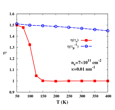
Figure 5: (Color online) Temperature dependence of the ratios of the momentum scattering rate (dashed curve) and the spin relaxation time (solid curve) with $n_{i}=3\times 10^{12}$ cm^-2 to those with $n_{i}=2\times 10^{12}$ cm^-2, labeled as $\eta(\tau_{p}^{-1})$ and $\eta(\tau_{s})$ respectively. $n_{e}=7\times 10^{11}$ cm^-2 and $\kappa=0.01$ nm^-1.

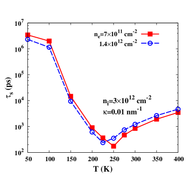
Figure 6: (Color online) Temperature dependence of spin relaxation time with different electron densities. Solid curve: $n_{e}=7\times 10^{11}$ cm^-2; Dashed curve: $n_{e}=1.4\times 10^{12}$ cm^-2. $n_{i}=3\times 10^{12}$ cm^-2 and $\kappa=0.01$ nm^-1.

While changing the impurity density influences the spin relaxation only at low temperature ($T<150$ K), the change of electron density is expected to affect spin relaxation in a large temperature regime, as both the intravalley and intervalley scatterings depend on the electron density. In fact, with the increase of electron density, the intravalley electron-impurity scattering is weakened while the intervalley electron-phonon scattering is strengthened. Therefore, with the increase of electron density, as long as the condition $l\ll\xi$ is satisfied, the spin relaxation time $\tau_{s}$ decreases in the weak intervalley scattering limit ($\tau_{s}\propto\tau_{p}^{-1}$ when $T\leq 100$ K and $\tau_{s}=\tau_{v}$ when $100<T\leq 250$ K) but increases in the strong intervalley scattering limit ($\tau_{s}\propto\tau_{v}^{-1}$ when $T>250$ K). We calculate the spin relaxation with a higher electron density $n_{e}=1.4\times 10^{12}$ cm^-2 and the impurity density $n_{i}=3\times 10^{12}$ cm^-2. For such case the electron mean free path $l$ has the largest value of 30 nm at $T=50$ K. In Fig. 6, we compare the spin relaxation for this case to the one with $n_{e}=7\times 10^{11}$ cm^-2 and $n_{i}=3\times 10^{12}$ cm^-2. It is indeed shown that with the increase of electron density, $\tau_{s}$ decreases when $T<250$ K but increases when $T\geq$250 K.

When the electron density is further increased and eventually $l\geq\xi$, the mechanism discussed in this work is not valid any more and the spin-flip scattering induced by the fluctuation of the SOC contributes to spin relaxation.glazov2157 ; sherman67 ; dugaev085306 ; zhangdpey When the latter is dominant, the spin relaxation time $\tau_{s}$ is of the order of 10 ns and insensitive to the temperature.dugaev085306 ; jeong

III.4 Anisotropy of spin relaxation without and with small perpendicular magnetic field

The above studies are limited to the spin relaxation along the $z$-axis. In fact, due to the in-plane effective magnetic field along ${\bf b}$, the spin relaxation time along any direction perpendicular to ${\bf b}$ is identical. Also, according to the simple model presented in the introduction, there is no spin relaxation along ${\bf b}$. However, due to the Rashba-type SOC, spins relax along ${\bf b}$ exponentially, with the spin relaxation time $\tau_{s}=\tau_{||}$ ($\tau_{||}$ can be obtained from $\tau_{\perp}$ given by the dotted curve in Fig. 4, as $\tau_{||}=2\tau_{\perp}$). This spin relaxation time is of the order of microseconds and insensitive to temperature. Due to the difference in spin relaxations along and perpendicular to ${\bf b}$, the spin relaxation in the plane parallel to ${\bf b}$, e.g., the graphene plane, is anisotropic. When the initial spin-polarization direction ${\bf n}$ deviates from ${\bf b}$ by an angle $\theta_{{\bf n},{\bf b}}$, the spin polarization along ${\bf n}$ relaxes in the form $P(t)=P(0)[\cos^{2}\theta_{{\bf n},{\bf b}}e^{-t/\tau_{||}}+\sin^{2}\theta_{{\bf n},{\bf b}}f(t)]$. Here $f(t)=\frac{e^{-t/\tau_{v}}}{\sqrt{1-(\omega\tau_{v})^{-2}}}\sin(\sqrt{\omega^{2}-\tau_{v}^{-2}}t+\phi)$ in the weak intervalley scattering limit $\tau_{\perp}^{-1}\ll\tau_{v}^{-1}\leq\omega$ ($100<T<250$ K) and $f(t)=e^{-\omega^{2}\tau_{v}t/2}$ in the strong intervalley scattering limit $\tau_{v}^{-1}\gg\omega$ ($T>250$ K), according to Eqs. (7) and (2) respectively.

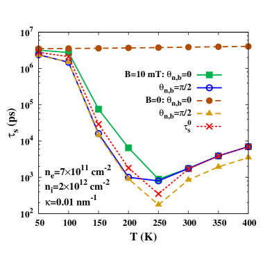
Figure 7: (Color online) Temperature dependence of spin relaxation time along different directions in the graphene plane with (solid curves) and without (dashed curves) an external magnetic field along the $z$-axis. Solid curve with squares (open circles): spin relaxation along the direction parallel (perpendicular) to ${\bf b}$ with external magnetic field of 10 mT along the $z$-axis; Dashed curve with closed circles (triangles): spin relaxation along the direction parallel (perpendicular) to ${\bf b}$ without external magnetic field. The dotted curve with crosses stands for the temperature dependence of the parameter, $\tau_{s}^{0}$, calculated from the average value of the spin relaxation rates along directions parallel and perpendicular to ${\bf b}$ without external magnetic field. $n_{e}=7\times 10^{11}$ cm^-2, $n_{i}=2\times 10^{12}$ cm^-2 and $\kappa=0.01$ nm^-1.

Usually, the spin relaxation in graphene is experimentally studied by the Hanle spin precession measurement.Tombros_08 ; han222109 ; Popinciuc ; Jozsa_09 ; han1012.3435 ; avsar ; jo ; Pi In such measurement, a small magnetic field ${\bf B}$ (at most of the order of 100 mT) perpendicular to the graphene plane is applied. Under the perpendicular magnetic field, the spin relaxations along different directions in the graphene plane are mixed. In the rippled graphene studied here, the spin relaxations along both ${\bf b}$ and the direction perpendicular to ${\bf b}$ are exponential in the strong intervalley scattering limit ($T>250$ K), with the two spin relaxation rates being $\tau_{||}^{-1}$ and $\omega^{2}\tau_{v}/2$, respectively. Therefore, when $B>\hbar|\tau_{||}^{-1}-\omega^{2}\tau_{v}/2|/(2g\mu_{B})$ (about 10 mT around room temperature), the spin relaxation along any direction in the graphene plane has the unique rate $\tau_{s}^{-1}=(\tau_{||}^{-1}+\omega^{2}\tau_{v}/2)/2\approx\omega^{2}\tau_{v}/4$.dohrmann147405 However, this is not the case in the weak intervalley scattering limit ($T<250$ K), as there is spin oscillation along the direction perpendicular to ${\bf b}$ [refer to Eq. (7)]. We apply a magnetic field of magnitude of 10 mT perpendicular to the graphene plane and calculate the spin relaxations along ${\bf b}$ ($\theta_{{\bf n},{\bf b}}=0$) and the direction perpendicular to ${\bf b}$ in the graphene plane ($\theta_{{\bf n},{\bf b}}=\pi/2$) respectively at different temperatures. The temperature dependence of the spin relaxation time along these two directions, with and without the perpendicular magnetic field, is plotted in Fig. 7. For comparison, we also plot the temperature dependence of the parameter, $\tau_{s}^{0}$, calculated from the average value of the perpendicular-magnetic-field–free spin relaxation rates along these two directions. It is shown that due to the perpendicular magnetic field, the spin relaxation becomes isotropic in the graphene plane when $T>250$ K, with $\tau_{s}^{-1}\approx\omega^{2}\tau_{v}/4$. However, when $T<250$ K, the anisotropy is strongly suppressed but not completely eliminated. Consequently, despite the angle $\alpha$ and the measured spin-polarization direction, the observed spin relaxation time in low-mobility rippled graphene by means of the Hanle spin precession measurement is expected to have a marked nonmonotonic dependence on temperature, with a minimum of several hundred picoseconds located around room temperature.

IV Conclusion and discussion

In conclusion, we have studied the electron spin relaxation in rippled graphene with low mobilities. The electron mean free path is smaller than the ripple size and the spin relaxation is determined by the local SOC induced by curvature. The curvature not only leads to the Rashba-type SOC, but also supplies a Zeeman-like term with opposite effective magnetic fields along graphene plane in two valleys.jeong We show that this Zeeman-like term, together with the intervalley electron-${\bf K}$-A${}_{1}^{\prime}$ optical phonon scattering, gives rise to a spin relaxation channel in rippled graphene at high temperature (with temperature $T>100$ K). This spin relaxation channel can cause a marked nonmonotonic dependence of spin relaxation on temperature along the direction perpendicular to the effective magnetic field from the Zeeman-like term. A minimal spin relaxation time of several hundred picoseconds is obtained around room temperature. However, the Rashba-type SOC dominates the spin relaxation along the effective magnetic field, leading to a temperature-insensitive spin relaxation time of the order of microseconds. Therefore, anisotropy exists in the spin relaxation in the graphene plane. In the presence of a small perpendicular magnetic field in Hanle spin precession experiment, the anisotropy of in-plane spin relaxation is strongly suppressed. Particularly, in the strong intervalley scattering limit, the spin relaxation in the graphene plane becomes isotropic, with the spin relaxation time being two times as large as that along the direction perpendicular to the effective magnetic field in the absence of the perpendicular magnetic field.

The spin relaxation channel revealed in this work manifests itself only when the electron mean free path is smaller than the ripple size. However, it is noted that when this spin relaxation channel is dominant (at temperature $T>100$ K), the spin relaxation is insensitive to the intravalley scattering, mainly contributed by the electron-impurity scattering in the low-mobility sample. It is also noted that in reality the ripples in graphene may not be quasi-periodic as proposed in this work. The radii of the curvatures may be spatial dependent.avsar Therefore, the observed spin relaxation is coherently averaged over the curvature morphology in the low-mobility sample.yzhourandom In such case, the spin relaxation is determined by the mean square of curvature in the zero and strong intervalley scattering limits. The spin relaxation channel revealed in this work should also exist in carbon nanotude. However, in the work of Semenov et al. where the spin relaxation in carbon nanotube was studied,semenov the intervalley scattering was not considered and this spin relaxation channel was not incorporated.

Finally, we discuss the experimentally observed spin relaxation in the low-mobility rippled graphene by Avsar et al..avsar In their sample with an electron density of $7.5\times 10^{11}$ cm^-2, the in-plane spin relaxation time obtained from the Hanle spin precession measurement increases mildly from about 130 to 150 ps when $T$ increases from 5 to 300 K.avsar Avsar et al. estimated the effect of the local SOC from curvature and excluded it from the spin relaxation mechanism (refer to the supplementary information of Ref. avsar, ). However, it is noticed that they only took into account the Rashba-type SOC according to Ref. Hernando_06, and the resulting spin relaxation time is naturally much longer than their experimental data. The spin relaxation channel revealed in this work supplies a possible origin of the experimentally observed short spin relaxation time around room temperature. To account for the experimental data in the whole temperature regime, some other factors, e.g., the randomly enhanced SOC by the substrate and/or adatoms,Castro_imp ; abde ; varykhalov ; zhanggraphene ; zhangdpey ; Fabian_SR may need to be considered.

- (1) K. S. Novoselov, A. K. Geim, S. V. Morozov, D. Jiang, Y. Zhang, S. V. Dubonos, I. V. Grigorieva, and A. A. Firsov, Science 306, 666 (2004).
- (2) A. K. Geim and K. S. Novoselov, Nature Mater. 6, 183 (2007).
- (3) N. Tombros, C. Józsa, M. Popinciuc, H. T. Jonkman, and B. J. van Wees, Nature (London) 448, 571 (2007).
- (4) F. Wang, Y. Zhang, C. Tian, C. Girit, A. Zettl, M. Crommie, and Y. Ron Shen, Science 320, 206 (2008).
- (5) C. W. J. Beenakker, Rev. Mod. Phys. 80, 1337 (2008).
- (6) A. H. Castro Neto, F. Guinea, N. M. R. Peres, K. S. Novoselov, and A. K. Geim, Rev. Mod. Phys. 81, 109 (2009).
- (7) N. M. R. Peres, Rev. Mod. Phys. 82, 2673 (2010).
- (8) D. S. L. Abergel, V. Apalkov, J. Berashevich, K. Ziegler, and T. Chakraborty, Adv. Phys. 59, 261 (2010).
- (9) Handbook of Spin Transport and Magnetism, edited by E. Y. Tsymbal and I. Žutić (CRC Press, Boca Raton, FL, 2011).
- (10) S. Das Sarma, S. Adam, E. H. Hwang, and E. Rossi, Rev. Mod. Phys. 83, 407 (2011).
- (11) M. Shiraishi and T. Ikoma, Physica E 43, 1295 (2011).
- (12) M. Acik and Y. J. Chabal, Jpn. J. Appl. Phys. 50, 070101 (2011).
- (13) A. K. Geim, Rev. Mod. Phys. 83, 851 (2011).
- (14) D. R. Cooper, B. D’Anjou, N. Ghattamaneni, B. Harack, M. Hilke, A. Horth, N. Majlis, M. Massicotte, L. Vandsburger, E. Whiteway, and V. Yu, arXiv:1110.6557.
- (15) N. Tombros, S. Tanabe, A. Veligura, C. Józsa, M. Popinciuc, H. T. Jonkman, and B. J. van Wees, Phys. Rev. Lett. 101, 046601 (2008).
- (16) W. Han, K. Pi, W. Bao, K. M. McCreary, Y. Li, W. H. Wang, C. N. Lau, and R. K. Kawakami, Appl. Phys. Lett. 94, 222109 (2009).
- (17) M. Popinciuc, C. Józsa, P. J. Zomer, N. Tombros, A. Veligura, H. T. Jonkman, and B. J. van Wees, Phys. Rev. B 80, 214427 (2009).
- (18) C. Józsa, T. Maassen, M. Popinciuc, P. J. Zomer, A. Veligura, H. T. Jonkman, and B. J. van Wees, Phys. Rev. B 80, 241403(R) (2009).
- (19) W. Han and R. K. Kawakami, Phys. Rev. Lett. 107, 047207 (2011).
- (20) A. Avsar, T. Y. Yang, S. Bae, J. Balakrishnan, F. Volmer, M. Jaiswal, Z. Yi, S. R. Ali, G. Güntherodt, B. H. Hong, B. Beschoten, and B. Özyilmaz, Nano Lett. 11, 2363 (2011).
- (21) S. Jo, D. K. Ki, D. Jeong, H. J. Lee, and S. Kettemann, Phys. Rev. B 84, 075453 (2011).
- (22) K. Pi, W. Han, K. M. McCreary, A. G. Swartz, Y. Li, and R. K. Kawakami, Phys. Rev. Lett. 104, 187201 (2010).
- (23) R. J. Elliott, Phys. Rev. 96, 266 (1954); Y. Yafet, Phys. Rev. 85, 478 (1952).
- (24) M. I. D’yakonov and V. I. Perel’, Zh. Éksp. Teor. Fiz. 60, 1954 (1971) [Sov. Phys. JETP 33, 1053 (1971)].
- (25) C. Ertler, S. Konschuh, M. Gmitra, and J. Fabian, Phys. Rev. B 80, 041405(R) (2009).
- (26) A. H. Castro Neto and F. Guinea, Phys. Rev. Lett. 103, 026804 (2009).
- (27) D. H. Hernando, F. Guinea, and A. Brataas, Phys. Rev. Lett. 103, 146801 (2009).
- (28) Y. Zhou and M. W. Wu, Phys. Rev. B 82, 085304 (2010).
- (29) J. S. Jeong, J. Shin, and H. W. Lee, Phys. Rev. B 84, 195457 (2011).
- (30) H. Ochoa, A. H. Castro Neto, and F. Guinea, arXiv:1107.3386.
- (31) V. K. Dugaev, E. Ya. Sherman, and J. Barnas, Phys. Rev. B 83, 085306 (2011).
- (32) P. Zhang and M. W. Wu, Phys. Rev. B 84, 045304 (2011).
- (33) P. Zhang and M. W. Wu, arXiv:1108.0283.
- (34) Y. A. Bychkov and E. I. Rashba, J. Phys. C 17, 6039 (1984).
- (35) D. H. Hernando, F. Guinea, and A. Brataas, Phys. Rev. B 74, 155426 (2006).
- (36) C. L. Kane and E. J. Mele, Phys. Rev. Lett. 95, 226801 (2005).
- (37) H. Min, J. E. Hill, N. A. Sinitsyn, B. R. Sahu, L. Kleinman, and A. H. MacDonald, Phys. Rev. B 74, 165310 (2006).
- (38) M. Gmitra, S. Konschuh, C. Ertler, C. A. Draxl, and J. Fabian, Phys. Rev. B 80, 235431 (2009).
- (39) S. Abdelouahed, A. Ernst, J. Henk, I. V. Maznichenko, and I. Mertig, Phys. Rev. B 82, 125424 (2010).
- (40) A. Varykhalov, J. S. Barriga, A. M. Shikin, C. Biswas, E. Vescovo, A. Rybkin, D. Marchenko, and O. Rader, Phys. Rev. Lett. 101, 157601 (2008).
- (41) J. S. Jeong and H. W. Lee, Phys. Rev. B 80, 075409 (2009).
- (42) W. Izumida, K. Sato, and R. Saito, J. Phys. Soc. Jpn. 78, 074707 (2009).
- (43) Y. G. Semenov, J. M. Zavada, and K. W. Kim, Phys. Rev. B 82, 155449 (2010).
- (44) E. Ya. Sherman, Phys. Rev. B 67, 161303 (2003).
- (45) M. M. Glazov, E. Ya. Sherman, and V. K. Dugaev, Physica E 42, 2157 (2010).
- (46) Y. Zhou and M. W. Wu, Europhys. Lett. 89, 57001 (2010).
- (47) M. W. Wu, J. H. Jiang, and M. Q. Weng, Phys. Rep. 493, 61 (2010).
- (48) M. W. Wu and H. Metiu, Phys. Rev. B 61, 2945 (2000).
- (49) M. W. Wu and C. Z. Ning, Eur. Phys. J. B 18, 373 (2000).
- (50) Y. Zhang, Z. Jiang, J. P. Small, M. S. Purewal, Y. -W. Tan, M. Fazlollahi, J. D. Chudow, J. A. Jaszczak, H. L. Stormer, and P. Kim, Phys. Rev. Lett. 96, 136806 (2006).
- (51) I. A. Luk’yanchuk and A. M. Bratkovsky, Phys. Rev. Lett. 100, 176404 (2008).
- (52) S. Adam and S. Das Sarma, Solid State Commun. 146, 356 (2008).
- (53) S. Fratini and F. Guinea, Phys. Rev. B 77, 195415 (2008).
- (54) E. H. Hwang and S. Das Sarma, Phys. Rev. B 77, 115449 (2008).
- (55) M. Lazzeri, S. Piscanec, F. Mauri, A. C. Ferrari, and J. Robertson, Phys. Rev. Lett. 95, 236802 (2005).
- (56) S. Döhrmann, D. Hägele, J. Rudolph, M. Bichler, D. Schuh, and M. Oestreich, Phys. Rev. Lett. 93, 147405 (2004).